Inconsistency of parsimony under the multispecies coalescent

Abstract

While it is known that parsimony can be statistically inconsistent under certain models of evolution due to high levels of homoplasy, the consistency of parsimony under the multispecies coalescent (MSC) is less well studied. Previous studies have shown the consistency of concatenated parsimony (parsimony applied to concatenated alignments) under the MSC for the rooted 4-taxa case under an infinite-sites model of mutation; on the other hand, other work has also established the inconsistency of concatenated parsimony for the unrooted 6-taxa case. These seemingly contradictory results suggest that concatenated parsimony may fail to be consistent for trees with more than 5 taxa, for all unrooted trees, or for some combination of the two. Here, we present a technique for computing the expected internal branch lengths of gene trees under the MSC. This technique allows us to determine the regions of the parameter space of the species tree under which concatenated parsimony fails for different numbers of taxa, for rooted or unrooted trees. We use our new approach to demonstrate that there are always regions of statistical inconsistency for concatenated parsimony for the 5- and 6-taxa cases, regardless of rooting. Our results therefore suggest that parsimony is not generally dependable under the MSC.

1 Introduction

One of the major goals of phylogenetics is to describe the relationships among organisms. We suppose the evolutionary relationship among $n$ species or taxa can be described by a rooted, binary and ultrametric species tree $\sigma=(\psi_{*},\bm{x})$ with $n$ tips, where $\psi_{*}$ denotes the rooted binary topology of the species tree and $\bm{x}$ gives the internal branch lengths of the species tree. The goal is to be able to infer the species tree $\sigma$, or some component of it, such as the topology $\psi_{*}$, using data available from the tip species.

The most common data used to infer species trees come from DNA sequences. DNA sequences are available from every gene (or locus) in a genome. Coalescent-based models give a probability distribution on the gene tree $G$ that represents the evolutionary history of a given locus among sampled individuals (Kingman, 1982). The gene tree topology $G$ at a locus is conditionally random given the species tree $\sigma$ when sampled individuals come from different species. The sequence data at this locus is then conditionally random given $G$, depending on any mutation events that have occurred on it. It is well-understood that the gene tree can be discordant (i.e. have internal branches that disagree) with the species tree for a number of biological reasons, such as introgression or horizontal gene transfer. However, arguably the most well-studied cause of gene tree discordance is incomplete lineage sorting (ILS), in which lineages in a population do not coalesce until entering a further ancestral population. In our analysis, we take ILS to be the sole cause of gene tree discordance, owing to the simplicity of mathematical models of ILS under the standard multispecies coalescent (MSC) model (Rannala et al., 2020). Recombination events along a chromosome allow neighboring loci to take on different gene tree topologies, all affected by the same biological processes. Accordingly, we assume that the gene tree $G$ at any given locus has a distribution given by the MSC for species tree $\sigma$. This distribution describes the probability distribution of the gene tree of a locus uniformly picked at random among a large number of loci.

ILS is particularly common when the internal branch lengths of the species tree are short. In some regions of the parameter space of the species tree (called the anomaly zone, or AZ for short), a discordant gene tree topology can be more likely to occur than one that matches the species tree topology (Degnan and Rosenberg, 2006). This demonstrates that even in an ideal world where we can infer gene tree topologies directly—essentially ignoring the randomness of sequences evolving on gene trees and the errors involved in inferring gene trees—a method that attempts to infer the species tree topology by simply returning the most common gene tree topology over many independent loci will be statistically inconsistent in some areas of parameter space. The fact that the most probable gene tree topology under the MSC is not in general the species tree topology might appear to doom so-called concatenation methods, which combine data from multiple loci into a single alignment. Such single alignments can be analyzed using a range of methods (e.g. parsimony, maximum likelihood, neighbor joining [NJ]) in order to return a tree or topology that optimizes a chosen cost function over the data. However, the regions of statistical consistency of such concatenation methods may differ from the AZ. For instance, simulations done in Kubatko and Degnan (2007) showed that, under the MSC, concatenated maximum-likelihood (ML) for 4 taxa could be consistent inside the AZ and inconsistent outside of it. This was shown more exhaustively in Mendes and Hahn (2018), who sampled a far greater number of points in parameter space.

Perhaps surprisingly, Liu and Edwards (2009) and Mendes and Hahn (2018) found that concatenated parsimony, assuming an infinite-sites mutation model and the MSC model, was statistically consistent for the rooted 4-taxa case across parameter space. These findings contrast with the well-known results described in Felsenstein (1978), which found an area of parameter space of statistical inconsistency of parsimony (sometimes called the Felsenstein zone). These two sets of results do not conflict, as inconsistency in the Felsenstein zone is caused by similarity due to homoplasy (multiple substitutions at a site), a phenomenon that does not occur in the infinite-sites model. It should also be noted that the analysis in Felsenstein (1978) does not incorporate gene tree discordance, while the results of Liu and Edwards (2009) and Mendes and Hahn (2018) do.

The success or failure of parsimony methods for cases with 5 or more taxa (“5+ taxa”), both in the rooted and unrooted cases, under coalescent-based models such as the MSC is not well-understood. Roch and Steel (2015) demonstrated inconsistency for the unrooted 6-taxon case under a general $r$-state mutation model, even when homoplasy is negligible. However, their results do not characterize the precise regions of parameter space where parsimony fails; instead, their model assumed the probability of coalescence in internal branches is sufficiently small, justifying the use of Ewens’ sampling formula in computing the probabilities of site patterns. To further explore regions of possible inconsistency of concatenated parsimony, we present a new method of calculating expected gene tree branch lengths. We first check that this framework agrees with the success of parsimony in the rooted 4-taxa scenario, providing a significantly easier proof of consistency in this case. Following this, we demonstrate that concatenated parsimony always has a region of inconsistency under the MSC and an infinite-sites model of mutation for rooted 5+ taxa. We conclude by discussing the implications of our results for the accurate inference of species trees.

2 Definitions

Following the notation of Degnan and Rosenberg (2006) and Rosenberg and Tao (2008), we think of a rooted, binary, and ultrametric species tree of $n$ tips as a pair $\sigma=(\psi_{*},\bm{x})$, where

• $\psi_{*}$ denotes the topology of $\sigma$ and is an element of the set ${\mathbb{T}}_{n}$ of all $n$ taxa rooted binary topologies. We use the $*$ subscript to denote that this is the true species tree topology. Generally, we will use $\psi$ without the $*$ subscript to denote a candidate topology.

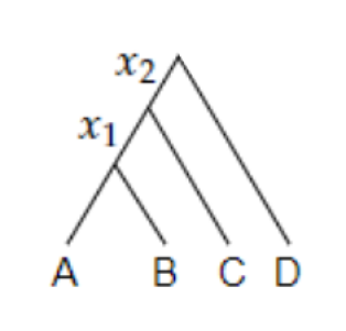
Figure 4: The tree $\sigma$ with topology $\psi_{*}=(((AB)C)D)$ and internal branch lengths $\bm{x}=(x_{1},x_{2})$

• $\bm{x}=(x_{1},\ldots,x_{n-2})\in\mathbb{R}^{n-2}_{+}$ denotes the $n-2$ internal branch lengths of $\sigma$, assigned in a depth-first manner (see Figures 4, 5 for examples). Because no coalescent events occur in the external branches (the $n$ branches containing the tips) of the species tree, their lengths are irrelevant to parsimony-based analyses and are thus omitted.

• The $n$ taxa are labeled by the set $[n]:=\{1,\ldots,n\}$. If $n$ is not too large, we often will write uppercase letters $\{A,B,C,...\}$ in place of numbers for clarity.

Note that for any choice of topology $\psi_{*}$ and internal branch lengths $\bm{x}$, we can find an ultrametric species tree with these internal branch lengths by letting the species tree have height $\sum_{i=1}^{n-2}x_{i}$, and choosing the external branch lengths so that the distance along any root to leaf path is equal to $\sum_{i=1}^{n-2}x_{i}$.

We consider the standard multispecies coalescent (MSC) model with $n$ species (Rannala and Yang, 2003; Rannala et al., 2020). Each population operates as an independent coalescent process during its existence in history. For simplicity, we assume also that the effective population size for all (ancestral) species are the same, and call it $N_{e}$. Hence there is a constant population size of $N_{e}$ diploid individuals within each ancestral population, and all branch lengths (the coordinates in $\bm{x}$) are measured in coalescent units of $2N_{e}$ generations under our MSC model. Now suppose we have sampled a sequence of unlinked loci in $n$ sampled individuals, one from each species. We assume that the unlinked loci, labeled by $\mathbb{N}=\{1,2,3,...\}$, are independent and identically distributed and are subject to the following assumptions:

• Each locus consists of a very large, essentially infinite, number of sites.

• The gene tree $G_{i}$ at locus $i$ is generated by the MSC on species tree $\sigma$.

• Mutations are selectively neutral, and arise on the gene tree $G_{i}$ according to an infinite-sites model of mutation with scaled mutation rate $\theta=4N_{e}\mu$, where $\mu$ is the per-generation mutation rate per locus.

  • $0$ refers to the ancestral allelic state at a site;

  • $1$ refers to the derived allelic state at a site.

• The alignment at locus $i$ is denoted by $A_{i}$. It consists of $n$ rows of nucleotides, one row for each sampled individual.

In concatenation methods, we take the finite set of alignments $A_{1},A_{2},...,A_{k}$ from loci $1,2,...,k$ and concatenate them, row by row for all the $n$ rows, into a single alignment $\mathcal{X}_{k}=A_{1}A_{2}\cdots A_{k}$ (Figure 1). We then attempt to make inferences based on the expense of explaining the alignment on a single candidate tree, according to a predetermined loss or ’cost’ function. Our hope is that as $k\to\infty$, the topology or other parameters of the candidate tree converges to that of the unknown species tree. Some methods, such as maximum-likelihood, use a cost function that depends on both the topology and branch lengths of the candidate tree. Here, we will examine methods where the cost function depends only on the topology $\psi$ of the candidate tree.

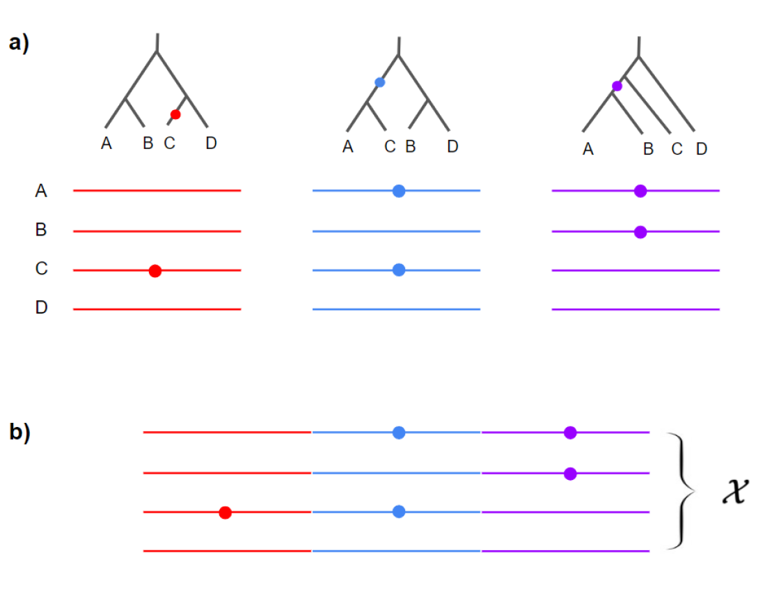
Figure 1: Illustration of the concatenation procedure. a) Three gene trees and alignments for $k=3$ independently evolving loci. Each mutation (circle) represents a $0\to 1$ (ancestral to derived) transition at a new site in the locus. Only one segregating site per locus is shown for simplicity. b) The resulting concatenated alignment $\mathcal{X}$, with three segregating sites.

We say a given site in the concatenated alignment $\mathcal{X}_{k}$ has site pattern $\chi$ if $\chi\subseteq[n]$ is the set of all tips with derived allelic type $1$ at the site. Clearly, there are $2^{n}$ possible site patterns for $n$ taxa. A site pattern $\chi$ is considered informative when $2\leq|\chi|\leq n-1$. Intuitively, informative site patterns (ISPs) carry information that helps to distinguish between topologies, since different number of mutations are needed to explain them for different topologies; see Figure 2 for an illustration. Accordingly, whenever we write a sum such as $\sum_{\chi}$, we mean to only sum over all ISPs, rather than all $2^{n}$ possible site patterns.

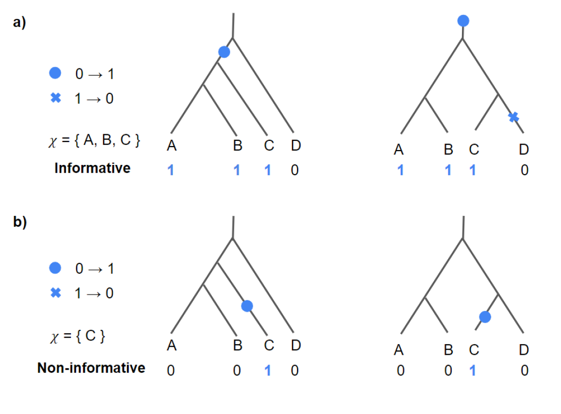
Figure 2: Illustration of a) informative site pattern (ISP), $\chi=\{A,B,C\}$ generated on two different tree topologies, with two different histories of mutation (one mutation for the topology on the left and two mutations for the topology on the right); and b) non-informative site pattern, $\chi=\{C\}$ on two different topologies, where the number of mutations are both one.

One natural approach to inference of the species tree topology from the concatenated alignment $\mathcal{X}_{k}$ is to associate a cost $c_{\psi}(\chi)$ for each topology $\psi\in\mathbb{T}_{n}$ and ISP $\chi$. We call these concatenated counting methods. The resulting estimator of the species tree topology is the $\psi\in\mathbb{T}_{n}$ that minimizes the overall cost over all informative sites in $\mathcal{X}_{k}$. That is, if the segregating sites in $\mathcal{X}_{k}$ are summarized by $\vec{\mathcal{N}}_{k}$ = $(\mathcal{N}_{k}(\chi))_{\chi}$, where $\mathcal{N}_{k}(\chi)$ is the number of sites with ISP $\chi$ in our data, then our estimator is

$$f(\vec{\mathcal{N}}_{k})=\underset{\psi\in\mathbb{T}_{n}}{\rm argmin}\left[\sum_{\chi}c_{\psi}(\chi)\mathcal{N}_{k}(\chi)\right].$$ (1)

Throughout this paper, if there is more than one choice for the argmin, then we pick one uniformly at random.

Under the infinite sites model of mutation, the expected number of mutations falling on a branch of a gene tree subtending $\chi$ is proportional to the length of the branch (each such mutation adds one to $\mathcal{N}_{k}(\chi)$). Thus the expected total cost per locus for the candidate topology $\psi$ is proportional to

$$C_{\sigma}(\psi):=\sum_{\chi}c_{\psi}(\chi)\ell_{\sigma}(\chi),$$ (2)

where $\ell_{\sigma}(\chi)=\ell_{(\psi_{*},\bm{x})}(\chi)$ is the expected length of an internal branch in the gene tree subtending $\chi$ under the MSC with species tree $\sigma$. In order for an estimator of this type to be statistically consistent – that is, $f(\vec{\mathcal{N}}_{k})$ converges to $\psi_{*}$ with probability $1$ as $k\to\infty$ – it is necessary (by the law of large numbers) that the expected total cost per locus $C_{\sigma}(\psi_{*})$ is less than the expected total cost per locus $C_{\sigma}(\psi)$ for any other topology $\psi\neq\psi_{*}$ in $\mathbb{T}_{n}$.

Parsimony methods, which assign costs $c_{\psi}(\chi)$ based on the minimum number of mutations needed to resolve site pattern $\chi$ on a tree with topology $\psi$, have been widely used in the existing literature. Depending on whether the ancestral state is known or not, parsimony can be used to attempt inference about (respectively) the rooted species tree topology or the unrooted species tree topology, as described below:

• Rooted parsimony: the cost $c_{\psi}(\chi)$ is the minimum number of mutations on topology $\psi$ (allowing back mutation $1\to 0$) needed to resolve $\chi$, assuming an ancestral state of $0$.

• Unrooted parsimony : the cost $c_{\psi}(\chi)$ is the minimum number of mutations on topology $\psi$ (allowing back mutation $1\to 0$) needed to resolve $\chi$, allowing the ancestral state to be $0$ or $1$.

Rooted parsimony usually requires the presence of an outgroup (with sufficient distance such that ILS is negligible between the $n$ taxa of interest and the outgroup) to distinguish between the ancestral and derived allelic states. For unrooted parsimony, the inability to distinguish the ancestral and derived states means that all pairs of rooted topologies $\psi_{1},\psi_{2}$ with identical unrooted topologies have $C_{\sigma}(\psi_{1})=C_{\sigma}(\psi_{2})$. Therefore, unrooted parsimony methods can only distinguish between topologies with different unrooted topologies. More generally, let ${\mathbb{T}}_{n}^{ur}$ denote the set of all $n$-taxon unrooted topologies. We can define a map ${\mathbb{T}}_{n}\to{\mathbb{T}}_{n}^{ur}$ by $\psi\mapsto\overline{\psi}$, where $\overline{\psi}$ denotes the unrooted topology of $\psi$. We say a concatenated cost method is unrooted if $c_{\psi_{1}}(\chi)=c_{\psi_{2}}(\chi)$ whenever $\overline{\psi_{1}}=\overline{\psi_{2}}$, such that the cost $c_{\overline{\psi}}(\chi)$ is well-defined in the sense it is invariant of the rooted representative $\psi$ of $\overline{\psi}$ that is chosen. The estimator of the unrooted species tree topology is then given by

$$f^{ur}(\vec{\mathcal{N}}_{k})=\underset{\overline{\psi}\in{\mathbb{T}}^{ur}_{n}}{\rm argmin}\left[\sum_{\chi}c_{\overline{\psi}}(\chi)\mathcal{N}_{k}(\chi)\right].$$ (3)

Note we usually exclude site patterns with $|\chi|=n-1$ in the unrooted case, since they no longer truly informative in this case. All such site patterns may be resolved by choosing the root to have state $1$, and including one $1\to 0$ mutation along a particular external branch.

3 Methods

3.1 Expected lengths of internal gene tree branches

In Mendes and Hahn (2018), expected internal branch lengths were calculated by conditioning on each individual gene tree topology, a technique that quickly becomes infeasible for larger $n$, since there are $(2n-3)!!=(2n-3)\times(2n-1)\times\cdots\times 1$ possible gene tree topologies. To get around this, we formulate a simpler, non-conditional technique to compute these expected lengths.

For an informative site pattern $\chi\in[n]$, we define the random variable $L(\chi)$ to be the length of the branch subtending exactly the members of $\chi$ in the random gene tree $G$ if this branch exists; otherwise it is defined to be $0$. Similarly, we can define the random variable $L^{+}(\chi)$ to be the sum of all branches in $G$ that subtend at least $\chi$ which we will refer to as the subtending length of $\chi$:

$$L^{+}(\chi)=\sum_{\eta\supseteq\chi}L(\eta).$$ (4)

By definition, we will take $L([n])=L^{+}([n])=0$, since we do not continue the gene tree above the MRCA of the $n$ samples. The primary observation is that the expected value of $L^{+}(\chi)$ under the probability distribution induced by species tree $\sigma$ is much easier to compute directly than the expected value of $L(\chi)$, as demonstrated in the following lemma.

Lemma 1.

For a given species tree $\sigma$, define $h(\sigma)$ to be the expected height of a gene tree with one sample from each taxon, and $h(\sigma_{\chi})$ to be the expected height of a gene tree with one sample from each of the taxa in $\chi$ only, both under the MSC on $\sigma$. The expected value of $L^{+}(\chi)$ under the MSC on $\sigma$ is

$$\ell^{+}_{\sigma}(\chi):={\mathbb{E}}_{\sigma}[L^{+}(\chi)]=h(\sigma)-h(\sigma_{\chi}),$$ (5)

The right hand side is well-defined in the sense that $h(\sigma)-h(\sigma_{\chi})$ only depends on internal branch lengths $\bm{x}$ of $\sigma$ whenever $2\leq|\chi|\leq n-1$.

Proof.

Note that $L^{+}(\chi)$ is exactly equal to the time $T_{[n]}$ of the MRCA of all of the $n$ samples, minus the time $T_{\chi}$ of the MRCA of the $|\chi|$ samples labeled by elements of $\chi$:

$$L^{+}(\chi)=T_{[n]}-T_{\chi}.$$ (6)

By taking expected values and noting that the time $T_{\chi}$ is independent of events involving lineages outside of $\chi$, the first claim follows. ∎

It is also easy to see that the distribution of $L^{+}(\chi)$ for $|\chi|\geq 2$ is independent of the external branch lengths of the species tree, since no coalescent events occur during them. Hence the expectation $\ell^{+}_{\sigma}(\chi)$ is also independent of the external branch lengths. To use Lemma 1, we apply the inclusion-exclusion principle to invert (4) and recover $L(\chi)$ in terms of the $L^{+}(\eta)$, as given in the following lemma (see Figure 3 for an illustration of this procedure)

Lemma 2.

For any fixed realization of the gene tree,

$$L(\chi)=\sum_{\eta\supseteq\chi}(-1)^{|\chi|-|\eta|}L^{+}(\eta).$$ (7)

Furthermore, the expected value of $L(\chi)$, with respect to the randomness of the gene tree under the MSC on $\sigma$, is equal to

$$\ell_{\sigma}(\chi):={\mathbb{E}}_{\sigma}[L(\chi)]=\sum_{\eta\supseteq\chi}(-1)^{|\chi|-|\eta|}\left[h(\sigma)-h(\sigma_{\chi})\right].$$

Proof.

The first claim follows since

$$\sum_{\eta\supseteq\chi}(-1)^{|\chi|-|\eta|}L^{+}(\eta) =\sum_{\eta\supseteq\chi}(-1)^{|\chi|-|\eta|}\sum_{\eta^{\prime}\supseteq\eta}L(\eta^{\prime})$$

$$=\sum_{\eta^{\prime}\supseteq\chi}L(\eta^{\prime})\sum_{\chi\subseteq\eta\subseteq\eta^{\prime}}(-1)^{|\chi|-|\eta|}$$

$$=\sum_{\eta^{\prime}\supseteq\chi}L(\eta^{\prime})1_{\{\eta^{\prime}=\chi\}}$$

$$=L(\chi)$$

since when $\eta^{\prime}\supsetneq\chi$, there are an equal number of sets $\eta$ with $\chi\subseteq\eta\subseteq\eta^{\prime}$ with $|\eta|\equiv|\chi|\mod 2$ and $|\eta|\equiv|\chi|+1\mod 2$. The second claim follows by taking expected values and applying Lemma 1.

∎

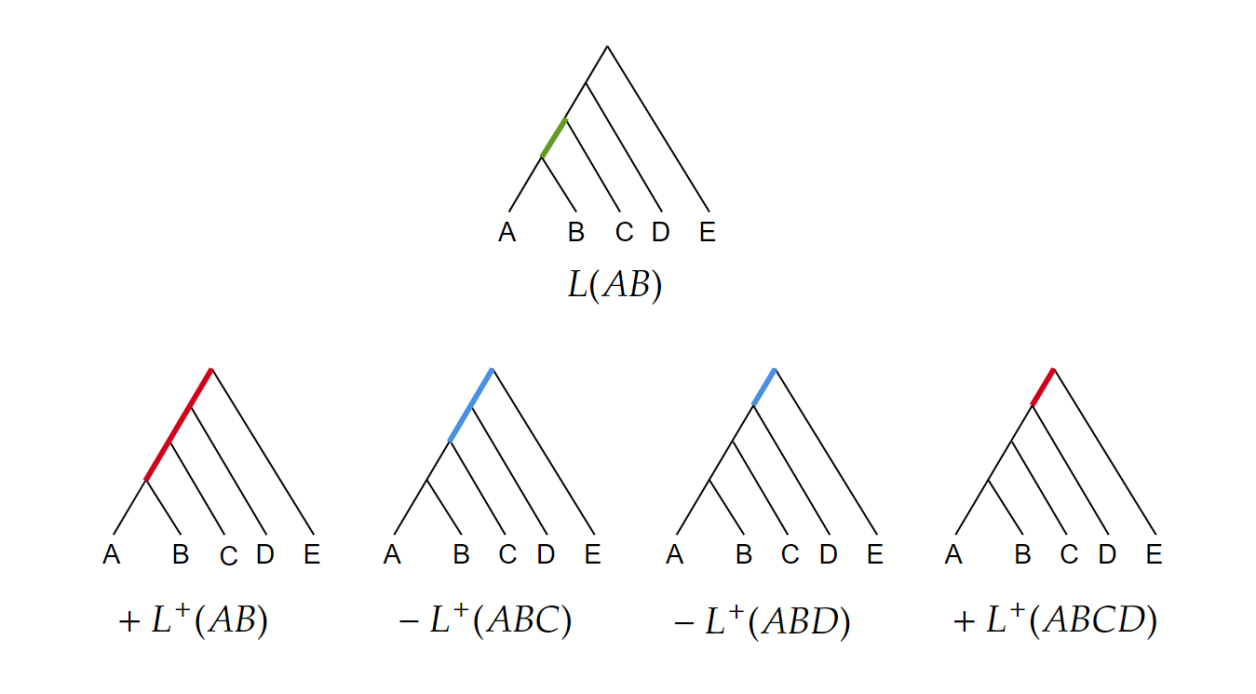
Figure 3: Illustration of recovering $L(\chi)$ for $\chi=\{A,B\}$ from $(L^{+}(\eta))_{\eta\supset\chi}$ on a realization of a 5-taxa tree. Terms with $L^{+}(\eta)=0$ for this realization, namely those with $E\in\eta$, are omitted.

However, it should be noted that when computing $C_{\sigma}(\psi)$, we only need to find a linear combination of the $\ell_{\sigma}(\chi)$. Thus, it is often easiest to first reverse the order of summation in $\sum_{\chi}\sum_{\eta\supseteq\chi}$, bypassing the need for the inversion procedure in Lemma 2. To illustrate this, we first let $T$ be any set of informative site patterns that is closed upwards (i.e. if $\chi\in T$ then $\eta\in T$ for all $\eta\supseteq\chi$). Then we can decompose

$$C_{\sigma}(\psi)=\sum_{\chi\notin T}c_{\psi}(\chi)\ell_{\sigma}(\chi)+\sum_{\chi\in T}c_{\psi}(\chi)\ell_{\sigma}(\chi)$$ (8)

and the second term can be rewritten as

$$=\sum_{\chi\in T}\sum_{\eta\supseteq\chi}(-1)^{|\chi|-|\eta|}c_{\psi}(\chi)\ell^{+}_{\sigma}(\eta)$$ (9)

$$=\sum_{\eta\in T}\ell^{+}_{\sigma}(\eta)\left(\sum_{\chi\subseteq\eta:\chi\in T}(-1)^{|\chi|-|\eta|}c_{\psi}(\chi)\right)$$ (10)

$$=\sum_{\eta\in T}\overline{c}^{T}_{\psi}(\eta)\ell^{+}_{\sigma}(\eta)$$ (11)

where we call $\overline{c}^{T}_{\psi}$ the dual costs of $c_{\psi}$ with respect to $T$. It is defined by (for each $\eta\in T$)

$$\overline{c}^{T}_{\psi}(\eta)=\sum_{\chi\subseteq\eta:\chi\in T}(-1)^{|\chi|-|\eta|}c_{\psi}(\chi)$$ (12)

Note that this definition may be inverted as before to yield the original costs for $\chi\in T$:

$$c_{\psi}(\chi)=\sum_{\eta\supseteq\chi}\overline{c}^{T}_{\psi}(\eta)$$ (13)

Therefore, choosing the original costs $\bm{c}=(c_{\psi}(\chi))_{\psi,\chi}$ is functionally equivalent to first selecting an upward-closed set of ISPs $T$, and choosing $(c_{\psi}(\chi))_{\psi,\chi\notin T}$ along with $(\overline{c}^{T}_{\psi}(\chi))_{\psi,\chi\in T}$. The numerical analysis of consistency of concatenated counting methods is often made simplest by working with the dual costs (particularly in the case where $T$ is taken to be all informative site patterns), since this is computationally inexpensive to find from the costs when $n$ is not large, and allows the direct use of the subtending lengths $\ell^{+}_{\sigma}(\chi)$.

3.2 Expected heights of gene trees

To calculate the expected height of a gene tree under a fixed species tree $\sigma$ with height $h_{\rm root}$, we must compute the probabilities $(p_{i})_{i=2}^{n}$ that exactly $i$ lineages of the gene tree enter the ancestral population of the $n$ species. These probabilities may be computed by a standard dynamic programming method, essentially a special case of the method used in Bryant et al. (2012), which we now describe.

Each internal node $v$ of the species tree $\sigma$ corresponds to a population, and the root corresponds to the ancestral population that is the most recent common ancestor of our sample. We let $R_{v}$ be the number of sample lineages in the gene tree that enter the ancestral population corresponding to node $v$. Then $p_{i}={\mathbb{P}}_{\sigma}(R_{\rm root}=i)$ by definition. Note also that for each of the $n$ external (tip) nodes, we have $R_{v}\equiv 1$. In the below, we compute the distribution of $\{R_{v}\}$, starting from the tips (which have value 1) and going up the species tree until we obtain the distribution of $R_{\rm root}$.

To this end, we consider the functions $g_{ij}(t)$ as defined in Tavaré (1984), defined to be the probability that $i$ lineages coalesce into $j\leq i$ lineages in a time interval of $t$ coalescent units under the standard coalescent process:

$$g_{ij}(t)=\sum_{k=j}^{i}e^{-k(k-1)t/2}\frac{(2k-1)(-1)^{j-k}j_{(k-1)}i_{[k]}}{k!(k-j)!i_{(k)}}$$ (14)

where $x_{(k)}=x(x-1)\cdots(x-k+1)$ denotes the falling factorial, and $x_{[k]}=x(x+1)\cdots(x+k-1)$ denotes the rising factorial.

Now, recall that $R_{v}\equiv 1$ for the $n$ external (tip) nodes. For the $n-2$ internal nodes, each of which (say $v$) has two descendant nodes $v_{1},v_{2}$, $R_{v}$ is equal to the sum of the lineages that remain after $R_{v_{1}}$- and $R_{v_{2}}$-many lineages coalesce in the ancestral populations corresponding to $v_{1}$ and $v_{2}$ respectively. Since the coalescent process in these ancestral populations are that of two independent Kingman coalescent process with $R_{v_{1}}$- and $R_{v_{2}}$-many tips respectively, it is clear that the probability generating function $f_{v}(z):={\mathbb{E}}_{\sigma}[z^{R_{v}}]$ of $R_{v}$ is given by

$$f_{v}(z)=\left(D_{t_{1}}f_{v_{1}}(z)\right)\cdot\left(D_{t_{2}}f_{v_{2}}(z)\right),$$ (15)

where $t_{m}$ $(m=1,2)$ is the length of the branch from $v$ to $v_{m}$, the $\cdot$ denotes standard polynomial multiplication in the variable $z$, and $D_{t}$ is the linear operator acting on the space of polynomials in the variable $z$ given by

$$D_{t}z^{i}=\sum_{j=1}^{i}g_{ij}(t)z^{j}.$$ (16)

The above procedure enables us to compute the distribution of $R_{\rm root}$.

Next, we obtain that the expected height of a gene tree is given by (Rannala and Yang, 2003; Rannala et al., 2020)

$$h(\sigma)=h_{\rm root}+\sum_{i=2}^{n}\left(2-\frac{2}{i}\right)p_{i},$$ (17)

since, conditional on $i$ lineages of the gene tree entering the MRCA of the $n$ species at time $h_{\rm root}$ in the past, the remaining genealogy agrees with that of a Kingman tree with $i$ tips, which has expected height $2-2/i$ (Kingman, 1982). Note that the probabilities $(p_{i})_{i=2}^{n}$ are independent of the labeling of the tips, so $h(\sigma)$ only varies between topologies with differing unlabeled topologies. One can also easily modify this procedure to compute the expected gene tree height of any restricted species tree $\sigma_{\chi}$. To do so, we simply remove all nodes in $\sigma$ that have descendants not in $\chi$, and join edges as necessary.

In practice, we let $\bm{x}$ vary, and think of $h(\sigma)=h(\psi_{*},\bm{x})$ as a function of $\bm{x}$. So the equation (17) for the expected height of the gene tree can be more suggestively written as

$$h(\psi_{*},\bm{x}) =h_{\rm root}(\bm{x})+\sum_{i=1}^{n}\left(2-\frac{2}{i}\right)p_{i}(\bm{x})$$

$$=h_{\rm root}(\bm{x})+P_{\psi_{*}}(\bm{X})$$ (18)

where $P_{\psi_{*}}(\bm{X})$ is a polynomial function in the transformed variables $\bm{X}:=(e^{-x_{1}},\ldots,e^{-x_{n-2}})$. Note this transformation is possible since the transition probabilities $g_{ij}(t)$ are polynomials in $e^{-t}$.

$n$	$\psi$	$P_{\psi}(\bm{X})$
$2$	$(XY)$	$1$
$3$	$((XY)Z)$	$1+\frac{X_{1}}{3}$
$4$	$(((XY)Z)U)$	$1+\frac{X_{2}}{3}+\frac{X_{1}X_{2}}{6}$
	$((XY)(ZU))$	$1+\frac{X_{1}}{3}+\frac{X_{2}}{3}-\frac{X_{1}X_{2}}{6}$
$5$	$((((XY)Z)U)V)$	$1+\frac{X_{3}}{3}+\frac{X_{2}X_{3}}{6}+\frac{X_{1}X_{2}X_{3}}{12}+\frac{X_{1}X_{2}^{3}X_{3}}{60}$
	$(((XY)Z)(UV))$	$1+\frac{X_{1}}{3}+\frac{X_{2}}{3}+\frac{X_{2}X_{3}}{6}-\frac{X_{1}X_{2}}{6}-\frac{X_{1}X_{2}X_{3}}{12}+\frac{X_{1}X_{2}^{3}X_{3}}{60}$
	$(((XY)(ZU))V)$	$1+\frac{X_{3}}{3}+\frac{X_{1}X_{3}}{6}+\frac{X_{2}X_{3}}{6}-\frac{X_{1}X_{2}X_{3}}{15}$

Table 1: Polynomials $P_{\psi}(\bm{X})$ for $2\leq n\leq 5$ taxa, with branch lengths $\bm{x}$

As mentioned previously, we only need to compute $P_{\psi}(\bm{X})$ for a single representative topology $\psi$ of each unlabeled topology up to $n$ taxa, since this polynomial function does not vary among trees with the same unlabeled topology. See Table 1 for reference. With (18), we can also easily compute the polynomial term in $h(\sigma_{\chi})$ by substituting variables appropriately in the expected gene tree height for the $|\chi|$-taxa topology that agrees with the topology of $\sigma_{\chi}$. Since we have not fixed external branch lengths of the species tree, one might object that terms such as $h_{\rm root}(\bm{x})$ lack precise definition. While this is true, in our final calculations, where we only consider differences such as $h(\sigma)-h(\sigma_{\chi})$, this issue disappears. Indeed, the difference in height between any two non-external nodes of the species tree, such as the root and the MRCA of species labeled by $\chi$, is well-defined and given by the length of the shortest path connecting these nodes, and so may be written as a linear combination of the internal branch lengths $x_{1},\ldots,x_{n-2}$.

3.3 Tests for statistical inconsistency

For a fixed $n$ and choice of costs $\bm{c}=(c_{\psi}(\chi))_{\psi,\chi}$, one simple method to demonstrate that there is a region of inconsistency is to consider the limit as $\bm{x}\to\bm{0}$, that is as the species tree $\sigma$ approaches a star tree. Regardless of our true species tree topology $\psi_{*}\in\mathbb{T}_{n}$, the expected total cost $C_{\sigma}(\psi)$ converges to a constant $S(\psi)$ dependent only on $\psi$, where the ’$S$’ is short for ’star tree’. In particular, it may be computed as

$$S(\psi)=\sum_{\chi}c_{\psi}(\chi)\cdot\frac{2}{|\chi|\binom{n}{|\chi|}}$$ (19)

since, for the Kingman coalescent with $n$ lineages, we have the expected lengths $\ell_{\sigma}(\chi)=2\left[|\chi|\binom{n}{|\chi|}\right]^{-1}$. This follows from Fu (1995) – the expected total length of branches subtending $i$ tips is $2/i$ – and exchangeability – there are $\binom{n}{i}$ possible branches of $i$ tips.

Therefore, if there exists $\psi\neq\psi_{*}\in{\mathbb{T}}_{n}$ such that $S(\psi)<S(\psi_{*})$, the cost-based method in question must be inconsistent in some neighborhood of $\bm{x}=\bm{0}$ for the topology $\psi_{*}$. In the unrooted case, we must additionally have that $\psi$, $\psi_{*}$ do not agree in unrooted topology to establish inconsistency. This argument will allow us to quickly establish inconsistency for parsimony for the rooted $5$- and unrooted $6$-taxa cases, which we examine in detail in the following sections.

We can also construct a generalization of the above argument by considering disjoint sets $\mathcal{A},\mathcal{B}\subseteq[n]$ with $\mathcal{A}\cup\mathcal{B}=[n]$. We let ${\mathbb{T}}_{n}(\mathcal{A}|\mathcal{B})\subseteq{\mathbb{T}}_{n}$ denote the set of all rooted $n$ taxon topologies that split $[n]$ into $\mathcal{A}$ and $\mathcal{B}$, i.e. all topologies $\psi\in{\mathbb{T}}_{n}$ for which the subtree restrictions of $\psi$ to $\mathcal{A}$ and $\mathcal{B}$ do not intersect (see (Allman et al., 2011) for a further discussion of splits).

In the following, when a function $\psi\mapsto F(\psi)$ is constant on ${\mathbb{T}}_{n}(\mathcal{A}|\mathcal{B})$, we say that $F(\psi)$ is invariant on ${\mathbb{T}}_{n}(\mathcal{A}|\mathcal{B})$.

Lemma 3.

Let $n\geq 3$ and fix a split $\mathcal{A}|\mathcal{B}$ of $[n]$. Then the estimator (1) with costs $\bm{c}=(c_{\psi}(\chi))_{\psi,\chi}$ is statistically consistent in the rooted case only if the followings hold:

1. $c_{\psi}(\mathcal{A})$ is invariant on ${\mathbb{T}}_{n}(\mathcal{A}|\mathcal{B})$ whenever $2\leq|\mathcal{A}|\leq n-1$,

2. $c_{\psi}(\mathcal{B})$ is invariant on ${\mathbb{T}}_{n}(\mathcal{A}|\mathcal{B})$ whenever $2\leq|\mathcal{B}|\leq n-1$,

3. $S_{\mathcal{A}|\mathcal{B}}(\psi)$ is invariant on ${\mathbb{T}}_{n}(\mathcal{A}|\mathcal{B})$ for any $\mathcal{A}\subseteq[n]$, where

   $$S_{\mathcal{A}|\mathcal{B}}(\psi)=\sum_{\chi\subsetneq\mathcal{A}}c_{\psi}(\chi)\frac{2}{|\chi|\binom{|\mathcal{A}|}{|\chi|}}+\sum_{\chi\subsetneq\mathcal{B}}c_{\psi}(\chi)\frac{2}{|\chi|\binom{|\mathcal{B}|}{|\chi|}}.$$ (20)

Proof.

To see that the quantity $c_{\psi}(\mathcal{A})$ must be invariant on ${\mathbb{T}}_{n}(\mathcal{A}|\mathcal{B})$ whenever $2\leq|\mathcal{A}|\leq n-1$, consider a species tree $\sigma$ with topology $\psi_{*}\in\mathcal{T}_{n}(\mathcal{A}|\mathcal{B})$ and all internal branch lengths equal to $0$, except the internal branch subtending $\mathcal{A}$, which we let have length $x$. We must have that $C_{\sigma}(\psi)$ is an invariant on ${\mathbb{T}}_{n}(\mathcal{A}|\mathcal{B})$, since $\sigma$ does not depend on the choice of $\psi_{*}\in{\mathbb{T}}_{n}(\mathcal{A}|\mathcal{B})$. Now we observe that

• As $x\to\infty$, $\ell_{\sigma}(\mathcal{A})=O(x)$, since with high probability, all tips of the gene tree labeled by $\mathcal{A}$ coalesce early in the internal branch in $\sigma$ subtending $\mathcal{A}$, and no other lineage may coalesce with this lineage for the rest of the internal branch.

• As $x\to\infty$, for any $\chi\neq\mathcal{A}$, $\ell_{\sigma}(\chi)=O(1)$, since an internal branch in the gene tree that subtends $\chi$ will always exist alongside at least one other lineage in the gene tree.

Therefore, the behavior of $C_{\sigma}(\psi)$ is dominated by the term $c_{\psi}(\mathcal{A})\ell_{\sigma}(\mathcal{A})$ as $x\to\infty$, and so we must have that $c_{\psi}(\mathcal{A})$ is an invariant for $\psi\in{\mathbb{T}}_{n}(\mathcal{A}|\mathcal{B})$ to ensure the invariance of $C_{\sigma}(\psi)$. The same argument establishes the invariance of $c_{\psi}(\mathcal{B})$ whenever $2\leq|\mathcal{B}|\leq n-1$.

To see the third quantity is invariant on ${\mathbb{T}}_{n}(\mathcal{A}|\mathcal{B})$, note that the split $\mathcal{A}|\mathcal{B}$ gives rise to a bipartition of each ISP $\chi$ by restriction, i.e $\chi=\mathcal{A}_{\chi}\cup\mathcal{B}_{\chi}$ where $\mathcal{A}_{\chi}=\mathcal{A}\cap\chi,\mathcal{B}_{\chi}=\mathcal{B}\cap\chi$. Now let $T$ be the set of all ISPs $\chi$ such that $|A_{\chi}|\geq 1$ and $|B_{\chi}\geq 1$. Clearly, $T$ is closed upwards, so we may use the alternative representation of $C_{\sigma}(\psi)$ using the dual costs with respect to $T$ as shown in the Methods section:

$$C_{\sigma}(\psi)=\sum_{\chi\notin T}c_{\psi}(\chi)\ell_{\sigma}(\chi)+\sum_{\chi\in T}\overline{c}^{T}_{\psi}(\chi)\ell^{+}_{\sigma}(\chi)$$ (21)

Now take $\sigma$ to be a species tree with topology $\psi_{*}\in{\mathbb{T}}_{n}(\mathcal{A}|\mathcal{B})$ with the branches subtending $\mathcal{A}$ and $\mathcal{B}$ having length $x$, and all other branch lengths equal to $0$. As before, since $\sigma$ does not depend on the choice of $\psi_{*}\in{\mathbb{T}}_{n}(\mathcal{A}|\mathcal{B})$, $C_{\sigma}(\psi)$ must be an invariant on ${\mathbb{T}}_{n}(\mathcal{A}|\mathcal{B})$.

Note that for any $\chi\in T$, as $x\to\infty$ with high probability the tips in the gene tree subtending $\mathcal{A}\cap\chi$ coalesce together before the root of the species tree, as do the tips subtending $\mathcal{B}\cap\chi$ – and conditional on these events occurring, the height of the gene tree matches with the height of the gene tree restricted to $\chi$. Thus, $\ell^{+}_{\sigma}(\chi)\to 0$ as $x\to\infty$, and the second term in 21 vanishes. To finish the argument, note that $\chi\notin T$ implies either $\chi\subseteq\mathcal{A}$ or $\chi\subseteq\mathcal{B}$. Using the previous fact that $c_{\psi}(\mathcal{A})$, $c_{\psi}(\mathcal{B})$ are invariants, we can ignore the terms $\chi=\mathcal{A},\mathcal{B}$ in the sum over $\chi\notin T$ in the first term of 21.

Finally, since as $x\to\infty$, the expected internal branch lengths $\ell_{\sigma}(\chi)$ for $\chi\subsetneq\mathcal{A}$ (resp. $\chi\subsetneq\mathcal{B}$) approaches that for the Kingman coalescent with $|\mathcal{A}|$ (resp. $|\mathcal{B}|$) tips. This completes the proof. ∎

3.4 Further implications for maximum-likelihood methods

As the number of loci $k$ sampled goes to infinity, the law of large numbers shows that the sample frequency of sites $\hat{p}_{k}(\eta)$ that have (informative) site pattern $\eta$ converges to

$$\hat{p}_{k}(\eta):=\frac{\mathcal{N}_{k}(\eta)}{\sum_{\chi}\mathcal{N}_{k}(\chi)}=\frac{\mathcal{N}_{k}(\eta)/k}{\sum_{\chi}\mathcal{N}_{k}(\chi)/k}\longrightarrow\frac{\ell_{\sigma}(\eta)}{\sum_{\chi}\ell_{\sigma}(\chi)}.$$ (22)

Calling the rightmost expression of the above $p_{\sigma}(\eta)$ (i.e the proportion of sites that have site pattern $\eta$ when averaging over the MSC on $\sigma$), this suggests a maximum-likelihood-esque method for joint inference of $\psi_{*}$ and internal branch lengths $\bm{x}$: namely the estimator

$$f_{MLE}(\vec{\mathcal{N}}_{k})=\underset{(\psi,\bm{y})\in\mathbb{T}_{n}\times\mathbb{R}_{+}^{n-2}}{\rm argmin}\left[-\sum_{\eta}\hat{p}_{k}(\eta)\log p_{\sigma}(\eta)\right].$$ (23)

Note this estimator could be extended to cases even where we do not assume an infinite-sites model of mutation, provided we have a method to estimate the average internal branch lengths across many gene trees in a given concatenated alignment. While it seems heuristically true that $f_{MLE}$ should be consistent as $k\to\infty$ by Gibbs’ inequality, rigorous proofs of consistency when the space of candidate trees is non-compact (i.e. ranging over all possible positive branch lengths) are much more difficult (RoyChoudhury et al., 2015). Furthermore, although it is known that the unrooted species tree topology is identifiable from site pattern frequencies (Chifman and Kubatko, 2015), a result that holds for more general reversible mutation models, it is not obvious that that the rooted species tree $\sigma$ is identifiable from the proportion of sites of having each site pattern. Thus we do not attempt a proof here.

4 Results

4.1 Theoretical results

Our main theoretical claims are given in the following theorems:

Theorem 1.

In the rooted 4-taxa case (resp. unrooted 5-taxa) case, for any species tree $\sigma=(\psi_{*},\bm{x})$ with nonzero branch lengths $\bm{x}$, rooted (resp. unrooted) parsimony is a statistically consistent estimator of $\psi_{*}$ (resp. $\overline{\psi}_{*}$) in the sense that the estimator (1) (resp. (3) converges to $\psi_{*}$ in probability (resp. $\overline{\psi_{*}}$) as $k\to\infty$.

Theorem 2.

In the rooted 5+ taxa case (resp. unrooted 6+ taxa) case, rooted (resp. unrooted) parsimony is a statistically inconsistent estimator: that is, there exists $\sigma=(\psi_{*},\bm{x})$ with $\psi_{*}\in{\mathbb{T}}_{5}$ (resp. $\psi_{*}\in{\mathbb{T}}_{6}$) such that under the MSC on $\sigma$, the estimator (1) (resp. (3) does not converge to $\psi_{*}$ in probability (resp. $\overline{\psi_{*}}$) as $k\to\infty$.

Put another way, Theorem 1 confirms the earlier result of Mendes and Hahn (2018), and extends it to the case of the unrooted $5$-taxa case, while Theorem 2 fills in the gap in theoretical knowledge about success/failure of parsimony in the rooted 5+ taxa case. Based on preliminary simulation results, we also hypothesize that Theorem 2 extends to any cost-based method, suggesting that the failure of parsimony in these cases is not due to a poor choice of costs, but rather a fundamental combinatorical difference between the rooted 4 taxa and 5+ taxa cases.

The primary advantage of our new technique, however, is that it not only allows us to prove the inconsistency of parsimony and other concatenated counting methods, but to visualize exactly where these methods fail. To do so, for a fixed species tree $\sigma=(\psi_{*},\bm{x})$, we define $K_{\sigma}$ to be the number of discordant topologies preferred by a given rooted cost-based method over the true species tree topology $\psi_{*}$ is the number of topologies for which $C_{\sigma}(\psi)<C_{\sigma}(\psi_{*})$:

$$K_{\sigma}:=\sum_{\psi\neq\psi_{*}}\mathbf{1}_{\{C_{\sigma}(\psi)<C_{\sigma}(\psi_{*})\}}.$$ (24)

In practice, we let $\bm{x}$ vary, and visualize $K_{\sigma}$ as a function of $\bm{x}$. When using concatenated parsimony (either rooted or unrooted), we will refer to trees that contribute to $K_{\sigma}$ as parsimony anomalous gene trees (PAGTs). In other words, PAGTs are topologies that concatenated parsimony prefers over the true species tree in some area of parameter space and under some costs.

4.2 Parsimony for rooted 4-taxa case

Here, we prove Theorem 1 regarding the consistency of parsimony for the rooted 4-taxa case in the special case of the unbalanced caterpillar tree $\psi_{*}=((AB)C)D)$, and show that it is always favored over the symmetric topology $\psi=((AB)(CD))$, the most likely gene tree topology in the anomaly zone. While a proof of consistency in this case already exists in Mendes and Hahn (2018), their method of proof involves rather tedious computations, in the sense that expected branch lengths are found by conditioning on all possible coalescent histories. We provide a simpler argument using the techniques outlined in the Methods section here.

To begin, since all discordant site patterns can be resolved by exactly $2$ mutations in the rooted 4-taxa case, it is most convenient to use the transformed costs $c^{\prime}_{\psi}(\cdot)=2-c_{\psi}(\cdot)$, which does not alter regions of consistency, provided we replace ”$\rm argmin$” by ”$\rm argmax$” in Equation 1, owing to the inclusion of the negative sign in the transformation. Indeed, the expected transformed cost $C^{\prime}_{\sigma}(\psi)$ per locus for topology $\psi$ satisfies

$$C^{\prime}_{\sigma}(\psi)=2\sum_{\chi}\ell_{\sigma}(\chi)-C_{\sigma}(\psi)$$ (25)

and the first term on the right hand side has no dependence on the chosen candidate topology $\psi$. In particular, for a species tree $\sigma=(\psi_{*},\bm{x})$ parsimony prefers the true species tree topology $\psi_{*}$ over an alternative one $\psi$ when

$$C^{\prime}_{\sigma}(\psi_{*})-C^{\prime}_{\sigma}(\psi)=\sum_{\chi\in\textrm{Con}(\psi_{*})}\ell_{\sigma}(\chi)-\sum_{\chi\in\textrm{Con}(\psi)}\ell_{\sigma}(\chi)>0$$ (26)

where $\textrm{Con}(\psi)$ denotes the set of all concordant ISPs on $\psi$, i.e. all site patterns that may be resolved by a single mutation on an internal branch of $\psi$. In our case, this amounts to

$$C^{\prime}_{\sigma}(\psi_{*})-C^{\prime}_{\sigma}(\psi) =[\ell_{\sigma}(ABC)+\ell_{\sigma}(AB)]-[\ell_{\sigma}(CD)+\ell_{\sigma}(AB)]$$ (27)

$$=\ell_{\sigma}(ABC)-\ell_{\sigma}(CD)$$ (28)

Now, we use (7) along with Lemma 1 to see that

$$\ell_{\sigma}(ABC) =\ell^{+}_{\sigma}(ABC)=h(\sigma)-h(\sigma_{ABC})$$ (29)

$$\ell_{\sigma}(CD) =\ell^{+}_{\sigma}(CD)-\ell^{+}_{\sigma}(ACD)-\ell^{+}_{\sigma}(BCD)$$ (30)

$$=[h(\sigma)-h(\sigma_{CD})]-2[h(\sigma)-h(\sigma_{ACD})]$$ (31)

In the last line we have substituted $\ell^{+}_{\sigma}(ACD)=\ell^{+}_{\sigma}(BCD)$, since $A$ and $B$ are sister species in $\sigma$. Using Table 1, we can read off

$$h(\sigma)-h(\sigma_{ABC}) =x_{2}+P_{(((AB)C)D)}(X_{1},X_{2})-P_{((AB)C)}(X_{1})$$ (32)

$$=x_{2}+\frac{X_{2}}{3}-\frac{X_{1}}{3}+\frac{X_{1}X_{2}}{6}$$ (33)

$$h(\sigma)-h(\sigma_{CD}) =P_{(((AB)C)D)}(X_{1},X_{2})-P_{(CD)}$$ (34)

$$=\frac{X_{2}}{3}+\frac{X_{1}X_{2}}{6}$$ (35)

$$h(\sigma)-h(\sigma_{ACD}) =P_{(((AB)C)D)}(X_{1},X_{2})-P_{((AC)D))}(X_{2})$$ (36)

$$=\frac{X_{1}X_{2}}{6}$$ (37)

Note that, in the last line, we substituted in $X_{2}$ for the argument of $P_{((AC)D)}$ since when restricting $\sigma$ to $ACD$, the sole internal branch has length $x_{2}$. Therefore

$$C^{\prime}_{\sigma}(\psi_{*})-C^{\prime}_{\sigma}(\psi) =\left[x_{2}+\frac{X_{2}}{3}-\frac{X_{1}}{3}+\frac{X_{1}X_{2}}{6}\right]-\left[\frac{X_{2}}{3}-\frac{X_{1}X_{2}}{6}\right]$$ (38)

$$=x_{2}+(X_{2}-1)\frac{X_{1}}{3}$$ (39)

since $\psi_{*},\psi$ both have an internal branch subtending $AB$, while $\psi_{*}$ has an internal branch subtending $ABC$, whereas $\psi$ has an internal branch subtending $CD$. To see that (38) is always greater than $0$ for $x_{1},x_{2}>0$, note that $X_{2}-1=e^{-x_{2}}-1>-x_{2}$ by Taylor’s theorem, so $C^{\prime}_{\sigma}(\psi_{*})-C^{\prime}_{\sigma}(\psi)>x_{2}(1-\frac{X_{1}}{3})$, which is positive for $x_{1},x_{2}>0$ since $X_{1}=e^{-x_{1}}<1$. This completes the proof.

While we have only demonstrated a particular case of Theorem 1 here, proving consistency when $\psi$ is any other topology in ${\mathbb{T}}_{4}$ or in the alternative case $\psi_{*}=((AB)(CD))$ and $\psi=((AB)C)D)$ is very similar, and is omitted here for brevity.

To prove consistency in general, it is sufficient to show that for each $\sigma=(\psi_{*},\bm{x})$, then $\ell_{\sigma}(\chi)\geq\ell_{\sigma}(\eta)$ whenever $\chi$ is concordant with $\psi_{*}$ and $\eta$ is discordant with $\psi_{*}$. This is primarily the result of a combinatoric coincidence that does not hold for $n\geq 5$, namely that under a star tree (i.e $\bm{x}\to\bm{0}$), $\ell_{\sigma}(\chi)$ is independent of $\chi$, since for any $\chi$ with $|\chi|=2$ and any $\eta$ with $|\eta|=3$, we have

$$\lim_{\bm{x}\to\bm{0}}\ell_{\sigma}(\chi)=\frac{2}{2\binom{4}{2}}=\frac{2}{3\binom{4}{3}}=\lim_{\bm{x}\to\bm{0}}\ell_{\sigma}(\eta)$$ (40)

and evidently, as we increase the internal branch lengths of $\sigma$, the expected length of a concordant site pattern increases faster than the expected length of a discordant one.

4.3 Parsimony for rooted 5-taxa case

Let $\psi_{1}=((((AB)C)D)E),\psi_{2}=(((AB)(CD))E),\psi_{3}=(((AB)C)(DE))$ be the labeled representatives of the three possible unlabeled topologies for $5$ taxa. These topologies, along with the depth-first assignment of branch lengths $\bm{x}$, are demonstrated in Figure 5. It is easy to argue directly that parsimony is inconsistent for 5 taxa by appealing to the limit $\bm{x}\to 0$ as explained previously:

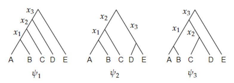
Figure 5: Representatives $\psi_{1},\psi_{2},\psi_{3}$ of the three unlabeled rooted topologies for 5 taxa, along with internal branch labels

$$S(\psi_{3})=\frac{43}{10}<\frac{13}{3}=S(\psi_{1})=S(\psi_{2})$$ (41)

In particular, for sufficiently short internal branch lengths, parsimony will always prefer trees with an unlabeled topology agreeing with $\psi_{3}$, even if the true unlabeled species tree topology matches with $\psi_{1}$ or $\psi_{2}$. We can see this in Figure 6, in which $\psi_{1}$ and $\psi_{2}$ have regions near $\bm{x}=\bm{0}$ with $15$ PAGTs, each of which is a labeled topology with unlabeled topology matching with $\psi_{3}$. Interestingly, there are no PAGTs when the true species tree is $\psi_{3}$, possibly because it is the maximally symmetric topology. Unfortunately, researchers do not know when this topology is the true one.

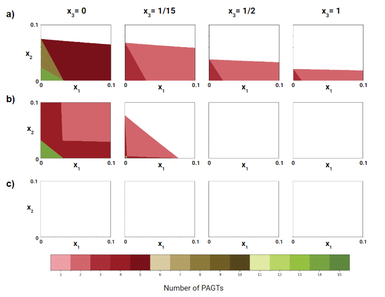
Figure 6: Number of topologies preferred by parsimony over the true species tree topology for a) $\psi_{1}$, b) $\psi_{2}$, c) $\psi_{3}$. Each column has a fixed value of $x_{3}$ (given in coalescent units), with $x_{1}$ and $x_{2}$ variable across $[0,0.1]$ coalescent units in each plot.

Figure 6 supports the intuition that as any internal branch length of the species tree is increased, the number of PAGTs monotonically decreases. In other words, increasing the internal branch lengths of the species tree only improves our ability to distinguish among topologies using parsimony. This is a highly desirable property of parsimony and other closely related variants, though it is not necessarily true for all possible choices of the costs $c_{\psi}(\cdot)$. As such, it warrants further theoretical investigation to understand exactly why parsimony has this property, but a full general proof seems challenging. Perhaps interestingly, when $\psi_{*}=(((AB)C)(DE))$ and the external branch length length $x_{3}$ leading to $(DE)$ is $0$, rooted parsimony always prefers the alternative symmetric topology $\psi=(((AB)(DE))C)$. This can be verified directly:

$$\,\,C_{\psi_{*},(x_{1},x_{2},0)}(\psi) =1+x_{1}+x_{2}+\frac{3}{2}(X_{1}+X_{2})+\frac{3}{10}X_{1}X_{2}$$ (42)

$$<\,\,C_{\psi_{*},(x_{1},x_{2},0)}(\psi_{*}) =1+x_{1}+x_{2}+\frac{3}{2}(X_{1}+X_{2})+\frac{1}{3}X_{1}X_{2}$$ (43)

This example demonstrates that we cannot in general guarantee the success of parsimony even when all but one of the internal branches is made arbitrarily large. Instead, we must have that all internal branch lengths exceed some critical threshold $x_{\rm min}$ to guarantee success for every topology. Numerically, we have found that for the 5-taxa case, a minimum branch length of $x_{\rm min}\approx 0.062205<1/15$ is needed to guarantee consistency for any topology, assuming again that the number of PAGTs is monotonically decreasing in each of the $x_{i}$.

As a side note, one might be tempted to ’fix’ parsimony in this case by normalizing the costs, i.e. by defining

$$c^{\prime}_{\psi}(\chi)=\frac{1}{S(\psi)}c^{\prime}_{\psi}(\chi)$$ (44)

such that all topologies are equally supported when the species tree is a star tree. However, as mentioned in the ”Theoretical results” section, preliminary simulation results suggest this does not lead to a consistent estimator, with topology $\psi_{3}$ having a wide variety of branch lengths for which this alternative form of parsimony is inconsistent.

4.4 Parsimony for unrooted 6-taxa case

Let $\overline{\psi}$ denote the unrooted topology corresponding to a rooted topology $\psi$. When computing the number of PAGTs in the unrooted case, the definition of the number of PAGTs, $K_{\sigma}$, should be updated to

$$K_{\sigma}:=\sum_{\overline{\psi}\neq\overline{\psi}_{*}}\mathbf{1}_{\{\overline{C}_{\sigma}(\overline{\psi})<\overline{C}_{\sigma}(\overline{\psi_{*}})\}}$$ (45)

where $\overline{C}_{\sigma}(\overline{\psi}):=C_{\sigma}(\psi)$. Note $\overline{C}_{\sigma}(\cdot)$ is well-defined: for unrooted parsimony, any $\psi_{1},\psi_{2}$ with the same unrooted topology $\overline{\psi}$ necessarily have $C_{\sigma}(\psi_{1})=C_{\sigma}(\psi_{2})$. We may again use the idea of reducing to a star tree to show the inconsistency of parsimony in this case: consider two unrooted topologies $\overline{\psi}_{1},\overline{\psi}_{2}$ with shapes as shown in Figure 7. Then it can be shown that the expected costs $S(\overline{\psi}_{1}),S(\overline{\psi}_{2})$ that arise when $\sigma$ is a star tree amount to

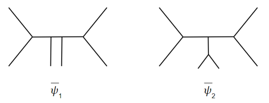
Figure 7: The two possible unrooted binary tree shapes for 6 taxa. Labels are omitted: $\overline{\psi}_{1}$ and $\overline{\psi}_{2}$ may be taken to be any unrooted labeled topologies with these respective shapes.

$$S(\overline{\psi}_{1})=\frac{28}{5}\neq\frac{167}{30}=S(\overline{\psi}_{2}).$$ (46)

Therefore, parsimony fails to be statistically consistent for the unrooted 6-taxa case under an infinite-sites model of mutation. Of course, this follows from the more general result of Roch and Steel (2015), since an infinite-sites model of mutation can be well-approximated by assuming the rate $\theta/2$ at which mutations fall on the gene tree is sufficiently small. Indeed, as a check of our results, we can recover equation 5 from Roch and Steel (2015), in which they demonstrated that, under a star tree, the parsimony score between $\overline{\psi}_{1}$ and $\overline{\psi_{2}}$ (denoted ’Z’ and ’Y’ in Roch and Steel (2015)) is

$$\frac{\theta}{60}+O(\theta^{2}).$$ (47)

This matches with our result, since we have

$$\frac{\theta}{2}\cdot\left[S(\overline{\psi}_{1})-S(\overline{\psi}_{2})\right]=\frac{\theta}{2}\cdot\frac{1}{30}=\frac{\theta}{60}.$$ (48)

Now, we consider more generally where parsimony is statistically inconsistent. It should be noted that even though candidate topologies only need be checked up to unrooted topology in computing $K_{\sigma}$, it is not in general true that two rooted species tree topologies with the same unrooted topology give rise to the same parsimony anomalous regions. To demonstrate this, in Figure 8 we visualize $K_{\sigma}$ for all $6$ possible unlabeled rooted topologies in the special case $\bm{x}=(x,\ldots,x)$; i.e. when all internal branch lengths of the species tree are identical.

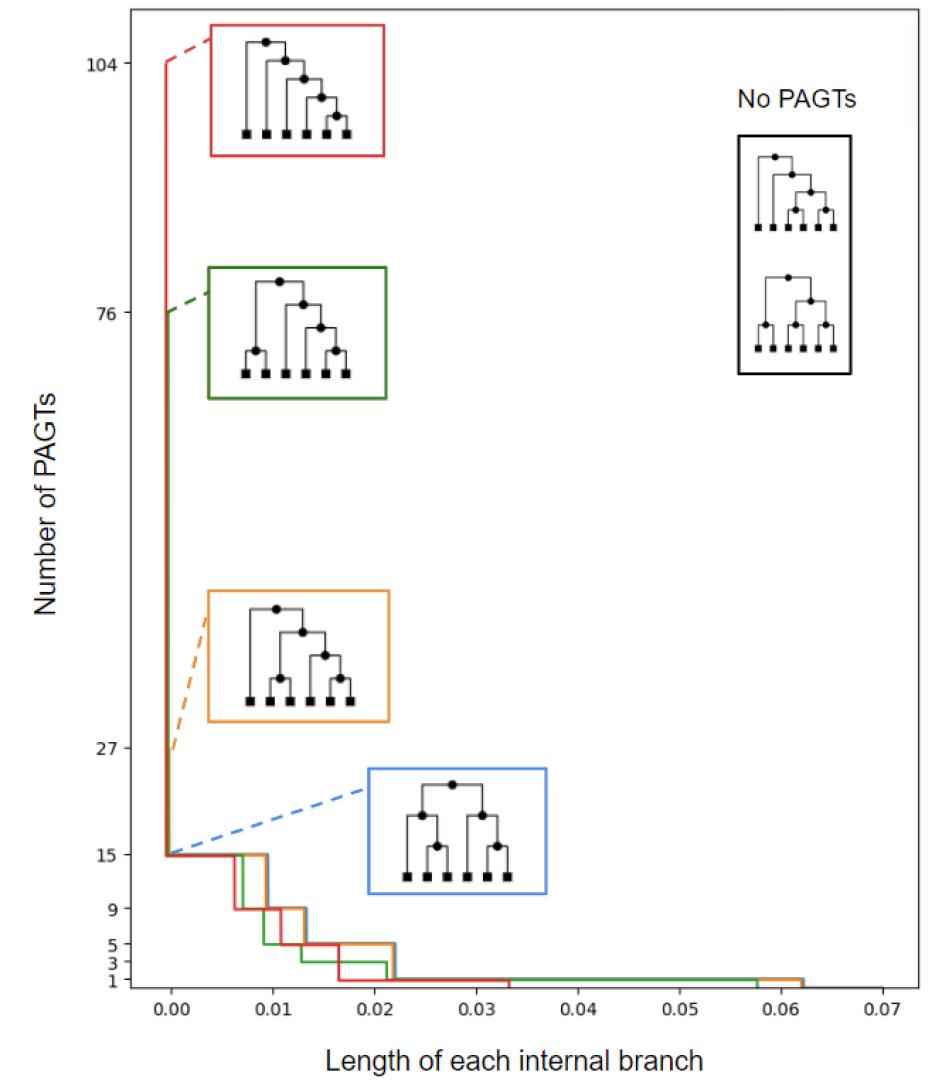
Figure 8: The number of parsimony anomalous gene trees (PAGTs) (vertical axis) for each possible rooted 6-taxa topology up to labeling, when all branch lengths have the same length (horizontal axis, coalescent units). Four topologies have any PAGTs, while two do not. The number of PAGTs when all branch lengths are $0$ is indicated for each of the four topologies with PAGTs by the connecting dotted lines (otherwise, these points are difficult to see). Images of topologies were generated in tskit (https://tskit.dev/tskit/docs/stable/) via the draw_svg() method. Overlapping lines have been moved slightly horizontally for visibility.

We can again see that, similar to the rooted 5-taxa case, once the minimum branch length exceeds $x_{\rm min}\approx 0.062205$, unrooted parsimony is guaranteed to be consistent for any unrooted 6-taxa topology. The numerical agreement of the $x_{\rm min}$ needed for consistency between the rooted 5-taxa and unrooted 6-taxa case is perhaps not terribly surprising: we conjecture that such a result holds true between the rooted $n$-taxa and unrooted $(n+1)$-taxa cases for all $n\geq 5$.

5 Discussion

Prior to the publication of Kubatko and Degnan (2007), maximum likelihood (ML) analyses of concatenated datasets dominated phylogenetics. However, the demonstration in Kubatko and Degnan (2007) that concatenated ML was inconsistent when ILS was high caused a huge explosion of research into methods that are robust to gene tree discordance (e.g. ASTRAL (Mirarab et al., 2014; Zhang et al., 2018), MP-EST (Liu et al., 2010), STAR Liu and Edwards (2009), SVDquartets (Chifman and Kubatko, 2014), etc). Rather than concatenate all loci, these methods instead consider each gene tree separately. Despite theoretical guarantees of consistency, such gene tree-based methods may suffer because of errors in inferring individual tree topologies from short sequences (Molloy and Warnow, 2018). Because longer (and likely therefore concatenated) alignments offer several advantages over shorter sequences (reviewed in Bryant and Hahn (2020)), there is still a desire for concatenation methods that are robust to ILS.

Results in both Liu and Edwards (2009) and Mendes and Hahn (2018) found that concatenated parsimony under an infinite-sites model was consistent when applied to rooted 4-taxon trees. It was therefore hoped that concatenated parsimony would be consistent when applied to more taxa (despite results on inconsistency of this same method on unrooted trees with 6+ taxa in Roch and Steel (2015)). The results presented here demonstrate that this hope was ill-founded: concatenated parsimony is not consistent on 5 or more taxa in the rooted case, or 6 or more taxa in the unrooted case. In this sense, the results found previously on 4 taxa appear to be more of a combinatorial coincidence than the beginning of a promising new approach. With only 4 taxa there are only two discordant gene trees, each of which requires at most a cost of two substitutions on the concordant topology; with more than 4 taxa there are many more discordant trees, each of which which may require more than two substitutions on the concordant topology. As a result, concatenated parsimony can favor the incorrect topology.

Although parsimony no longer appears to be a viable option for consistent inference from concatenated data, there are other options. For instance, both Liu and Edwards (2009) and Mendes and Hahn (2018) also found that concatenated neighbor joining (NJ) was consistent on rooted 4-taxa trees in the presence of high ILS. Although no results were presented for more than 4 tips (or on unrooted trees), it is expected that NJ will continue to be consistent for all tree sizes as it is based on expected coalescence times. However, distance methods such as NJ are prone to inconsistency when homoplasy is high (e.g. in the Felsenstein zone), so this will not be a dependable approach in all of parameter space. As an alternative, the mixtures across sites and trees (MAST) model of Wong et al. (2024) has all of the advantages of concatenated ML, but allows the alignment to come from a set of alternative topologies. This approach has been found to be consistent in simulations, but more theoretical work is needed to prove its consistent more broadly.

In order to provide evidence that concatenated parsimony is not consistent on 5+ taxa, we have introduced a new mathematical method for estimating the total length of branches subtending a sub-tree. Under an infinite-sites model, this total length is proportional to the number of informative site patterns in a concatenated alignment across all gene trees (Mendes and Hahn, 2018). While this method may have further uses, it is important to point out that its relevance here depends on the infinite-sites assumption. Future work using alternative mutation models (e.g. Jukes-Cantor) may allow our approach to be used in a wider range of scenarios and to be compared directly with work using alternative approaches (Roch and Steel, 2015). Finally, new techniques such as the maximum-likelihood method mentioned in the section on“Further implications…” that attempt to jointly infer species tree topology and internal branch lengths from estimated lengths of internal branches in gene trees provides an avenue for future theoretical and experimental exploration.

CRediT authorship contribution statement

D.A. Rickert: Methodology, Software, Formal Analysis, Investigation, Visualization, Writing - Original Draft, Writing - Review & Editing. W.-T. Fan: Writing - Review & Editing, Formal Analysis, Funding acquisition. M.W. Hahn: Conceptualization, Methodology, Writing - Original Draft, Writing - Review & Editing, Supervision, Project Administration, Funding acquisition.

Conflicts of interest

The authors declare no conflicts of interest.

References

- Allman et al. (2011) Allman, E.S., Degnan, J.H., Rhodes, J.A., 2011. Identifying the rooted species tree from the distribution of unrooted gene trees under the coalescent. Journal of mathematical biology 62, 833–862.
- Bryant et al. (2012) Bryant, D., Bouckaert, R., Felsenstein, J., Rosenberg, N.A., RoyChoudhury, A., 2012. Inferring species trees directly from biallelic genetic markers: bypassing gene trees in a full coalescent analysis. Molecular Biology and Evolution 29, 1917–1932.
- Bryant and Hahn (2020) Bryant, D., Hahn, M.W., 2020. The multispecies coalescent model and species tree inference, in: Scornavacca, C., Delsuc, F., Galtier, N. (Eds.), Phylogenetics in the Genomic Era. Self Published. chapter 3.4, pp. 3.4:1–3.4:23.
- Chifman and Kubatko (2014) Chifman, J., Kubatko, L., 2014. Quartet inference from snp data under the coalescent model. Bioinformatics 30, 3317–3324.
- Chifman and Kubatko (2015) Chifman, J., Kubatko, L., 2015. Identifiability of the unrooted species tree topology under the coalescent model with time-reversible substitution processes, site-specific rate variation, and invariable sites. Journal of Theoretical Biology 374, 35–47.
- Degnan and Rosenberg (2006) Degnan, J.H., Rosenberg, N.A., 2006. Discordance of species trees with their most likely gene trees. PLoS Genetics 2, e68.
- Felsenstein (1978) Felsenstein, J., 1978. Cases in which parsimony or compatibility methods will be positively misleading. Systematic Zoology 27, 401–410.
- Fu (1995) Fu, Y.X., 1995. Statistical properties of segregating sites. Theoretical Population Biology , 172–197.
- Kingman (1982) Kingman, J.F.C., 1982. The coalescent. Stochastic Processes and their Applications 13, 235–248.
- Kubatko and Degnan (2007) Kubatko, L., Degnan, J., 2007. Inconsistency of phylogenetic estimates from concatenated data under coalescence. Systematic Biology 56, 17–24.
- Liu and Edwards (2009) Liu, L., Edwards, S.V., 2009. Phylogenetic analysis in the anomaly zone. Systematic Biology 58, 452–460.
- Liu et al. (2010) Liu, L., Yu, L., Edwards, S.V., 2010. A maximum pseudo-likelihood approach for estimating species trees under the coalescent model. BMC evolutionary biology 10, 302.
- Mendes and Hahn (2018) Mendes, F.K., Hahn, M.W., 2018. Why concatenation fails near the anomaly zone. Systematic Biology 67, 158–169.
- Mirarab et al. (2014) Mirarab, S., Reaz, R., Bayzid, M.S., Zimmermann, T., Swenson, M.S., Warnow, T., 2014. Astral: genome-scale coalescent-based species tree estimation. Bioinformatics 30, i541–i548.
- Molloy and Warnow (2018) Molloy, E.K., Warnow, T., 2018. To include or not to include: the impact of gene filtering on species tree estimation methods. Systematic biology 67, 285–303.
- Rannala et al. (2020) Rannala, B., Leache, A., Edwards, S., Yang, Z., 2020. The multispecies coalescent model and species tree inference, in: Scornavacca, C., Delsuc, F., Galtier, N. (Eds.), Phylogenetics in the Genomic Era. Self Published. chapter 3.3, p. 3.3:1–3.3:21.
- Rannala and Yang (2003) Rannala, B., Yang, Z., 2003. Bayes estimation of species divergence times and ancestral population sizes using dna sequences from multiple loci. Genetics 164, 1645–1656.
- Roch and Steel (2015) Roch, S., Steel, M., 2015. Likelihood-based tree reconstruction on a concatenation of aligned sequence data sets can be statistically inconsistent. Theoretical Population Biology 100, 56–62.
- Rosenberg and Tao (2008) Rosenberg, N.A., Tao, R., 2008. Discordance of species trees with their most likely gene trees: the case of five taxa. Systematic Biology 57, 131–140.
- RoyChoudhury et al. (2015) RoyChoudhury, A., Willis, A., Bunge, J., 2015. Consistency of a phylogenetic tree maximum likelihood estimator. Journal of Statistical Planning and Inference 161, 73–80.
- Tavaré (1984) Tavaré, S., 1984. Line-of-descent and genealogical processes, and their applications in population genetics models. Theoretical Population Biology 26, 119–164.
- Wong et al. (2024) Wong, T.K., Cherryh, C., Rodrigo, A.G., Hahn, M.W., Minh, B.Q., Lanfear, R., 2024. Mast: Phylogenetic inference with mixtures across sites and trees. Systematic Biology , syae008.
- Zhang et al. (2018) Zhang, C., Rabiee, M., Sayyari, E., Mirarab, S., 2018. Astral-iii: polynomial time species tree reconstruction from partially resolved gene trees. BMC bioinformatics 19, 15–30.