Optimizing Information Access in Networks via Edge Augmentation

Abstract

Given a graph $G=(V,E)$ and a model of information flow on that network, a fundamental question is to understand if all the nodes have sufficient access to information generated at other nodes in the graph. If not, we can ask if a small set of “interventions” in the form of edge additions improve information access. Formally, the broadcast value of a network is defined to be the minimum over pairs $u,v\in V$ of the probability that an information cascade starting at $u$ reaches $v$. Recent work in the algorithmic fairness literature [2] has focused on heuristics for adding a few edges to a graph to improve its broadcast. Our goal in this paper is to formally study the approximability of this problem, termed Broadcast Improvement. Given $G$ and a parameter $k$, the goal is to find the best set of $k$ edges to add to $G$ in order to maximize the broadcast value of the resulting graph.

We develop efficient bicriteria approximation algorithms for this problem. If the optimal solution adds $k$ edges and achieves a broadcast of $\beta^{*}$, we develop algorithms that can (a) add $2k-1$ edges and achieve a broadcast value roughly $(\beta^{*})^{4}$, or (b) add $O(k\log n)$ edges and achieve a broadcast roughly $\beta^{*}$. We also provide other trade-offs, that can be better depending on $k$ and the parameter associated with propagation in the cascade model. We complement our results by proving that unless P=NP, any algorithm that adds $O(k)$ edges must lose significantly in the approximation of $\beta^{*}$, resolving an open question.

Our techniques are inspired by the connections between Broadcast Improvement and problems such as Metric $k$-Center and Diameter Reduction. However, since the objective involves information cascades, we need to develop novel probabilistic tools to reason about existence of paths in edge-sampled graphs. Finally, we show that our techniques extend to a single-source variant of the problem, where we focus on adding edges to a graph to maximize the information access of a given node $v_{s}$. Analogous to Broadcast Improvement, we show both bicriteria algorithms and inapproximability results.

1 Introduction

There has been significant recent work on computational questions around fairness in information access on social networks [16, 30, 27, 1, 21, 3, 4, 30, 28, 22, 25], based on characterizing this access in terms of the probability of transmission under some stochastic model for information spread. While much of the literature focuses on intervening in the network by augmenting a seed set of nodes (which initially possess the information) in order to maximize the probability that other nodes receive it, a recent line of work [2, 21, 29] has considered the problem of improving information access in networks by adding edges.

In particular, [2] considers the setting where access to information from all nodes in the network is equally important. To do this, they define several measures of advantage based on the information access signatures [5], which record the pairwise probabilities that nodes can share information with one another under some model of information flow. Specifically, they focus on improving the broadcast, defined to be the minimum pairwise access probability over all pairs of nodes in the network under the standard probabilistic model of influence propagation, Independent Cascade [24], with a uniform transmission probability $\alpha$. While originally defined as an iterative process for activating nodes and propagating information along edges, the probability of two nodes sharing information under Independent Cascade is equivalent to the probability that they are in the same connected component in a graph generated by adding each edge in the input independently with probability $\alpha$. We also refer to the access probability as proximity; see Section 2 for formal definitions.

Specifically, in [2], Bashardoust et al. design and empirically evaluate several heuristics for finding $k$ edges whose addition leads to the largest broadcast value (a problem we refer to as Broadcast Improvement). They leave open whether this problem is NP-hard, and do not prove quality guarantees for any of the introduced heuristics.

More broadly, this work is related to network design, an area that has seen significant work in both the Data Mining and Theoretical Computer Science communities. Especially relevant to our work are results on edge augmentations that improve various connectivity metrics associated with nodes (see, e.g., [6, 26, 9]). From a techniques perspective, we also draw insights from prior algorithms for Diameter Reduction [11, 7], which can be viewed as the analogue of our problem when the information access between two vertices is modeled as shortest path distance. This is part of a much larger literature on the parameterized complexity of edge modification to achieve various graph properties; we refer the reader to the recent survey by Crespelle et. al. for an overview [10].

1.1 Our Results

Our main algorithmic results are on the Broadcast Improvement problem, where we are given a parameter $k$ and the goal is to compete with the optimal broadcast possible by adding $k$ edges to $G$. Denoting this optimal broadcast by $\beta^{*}$, we give bicriteria algorithms that trade off between the number of edges added and the obtained broadcast value. In our algorithms, we also take care in optimizing the dependence on the parameter $\alpha$, the edge activation parameter (probability with which information spreads across an edge). This is because depending on the application and network structure, information graphs have been used with a range of values for $\alpha$, from around $0.01$ [5] to $0.6$ [2]. We obtain several algorithms which offer trade-offs between $\alpha$ and $1/k$. A short summary of the results is presented in Table 1.

Table 1: Outline of approximation bounds given that optimal broadcast achievable by adding $k$ edges is $\beta^{*}$.

Algorithm	Number of Edges Added	Broadcast Guarantee
$k$-center-based	$2k-1$	$\frac{(\beta^{*})^{4}\alpha^{2}}{(1+2k\alpha)^{4}}$
Constant witness I	$O(k^{2}\log n)$	$\Omega\left(\frac{\beta^{*}}{k^{4}}\right)$
Constant witness II	$O(k^{2}\log n)$	$\Omega\left(\frac{\beta^{*}\alpha}{k^{2}}\right)$
Submodularity-based	$O(\frac{k}{\varepsilon}\log n)$	$\Omega\left(\frac{\beta^{*}\alpha^{2+\varepsilon}}{k^{2}}\right)$ ($\forall\varepsilon>0$)

Algorithms for Broadcast Improvement. We present three techniques:

• We establish a relationship between Broadcast Improvement and Metric $k$-Center. Using this, we show that an analog of the ball-growing algorithm for Metric $k$-Center can also be used for Broadcast Improvement. If we have a guess $x$ for $\beta^{*}$ and we construct a maximal set of balls of “radius” approximately $x$, we prove that any optimal solution must have at least one endpoint in each ball; the centers of the balls can then be used to produce an approximate solution, leading to an algorithm that outputs $(2k-1)$ edges whose addition results in a graph with broadcast value roughly $(\beta^{*})^{4}$. See Section 3 for details.

• We then study how to add edges so as to obtain broadcast linear in $\beta^{*}$. For this, we first establish that there exists a near-optimal solution that has a special structure, that we refer to as a constant witness. We leverage two kinds of structure (optimized for different regimes of $k,\alpha$), and show that this leads to an algorithm with one of two guarantees, (i) add $O(k^{2}\log n)$ edges and guarantee broadcast of $\frac{\beta^{*}\alpha}{k^{2}}$, or (ii) add $O(k^{2}\log n)$ edges and guarantee broadcast of $\frac{\beta^{*}}{k^{4}}$, up to constants. See Section 4 for details.

• Our final technique is based on submodularity. As we note in 1, the pairwise access probability between two nodes as a function of the added edges is not submodular, but we argue that for subsets of edges forming a star, access to the center of the star possesses a submodularity property! We leverage this to obtain a solution that adds only $O(k\log n)$ edges, and guarantees broadcast of $\frac{\beta^{*}\alpha^{2+\varepsilon}}{k^{2}}$ for any $\varepsilon>0$. See Section 5 for details.

Our connection to Metric $k$-Center is modular, so it allows us to obtain an improvement over our results in Section 3 under an appropriate doubling-dimension assumption. We refer to Theorem 3 for the details.

Hardness of Broadcast Improvement. In  Section 6, we provide complementary hardness results. Specifically, we prove that unless P=NP, no efficient algorithm that outputs $O(k)$ edges can guarantee a broadcast better than $(\beta^{*})^{6/5-\varepsilon}$. This provides evidence that the $\log n$ overhead in the number of edges in Section 5 cannot be avoided.

Single Source Variant. Finally, we also study the single-source version of Broadcast Improvement, which we call Reach Improvement. Here the goal is to maximize the access of a given vertex to all the other vertices (see Section 2 for a formal definition). Analogous single-source variants of diameter minimization have been studied in the literature [11].

We start with a black-box reduction showing that any algorithm for Broadcast Improvement can be converted into an algorithm for Reach Improvement, with a loss of a square in the objective value. However, this does not yield the best bounds; by modifying our methods, we show a direct algorithm for Reach Improvement that adds $O(k\log n)$ edges, and ensures an objective value of $\max\{\frac{\Upsilon^{*}\alpha}{1+k\alpha},\frac{\Upsilon^{*}}{k}\}$, where $\Upsilon^{*}$ is the optimum objective value. We then show a hardness result that rules out algorithms that output $O(k)$ edges and achieve an objective value better than $(\Upsilon^{*})^{4/3-\varepsilon}$. See Section 7 for details.

2 Preliminaries

We use standard graph-theoretic definitions and notations throughout. Given a graph $G=(V,E)$ and a set $S\subseteq V^{2}\setminus E$, we write $G+S=(V,E\cup S)$ to denote the graph formed by adding the edges $S$ to $G$. For a positive integer $n$, we use the notation $[n]=\{1,2,\ldots,n\}$ for the set of integers from $1$ to $n$. Unless otherwise specified, all logarithms have base $2$. When discussing a probability event $\mathcal{E}$, we use the notation $\bar{\mathcal{E}}$ to indicate the complement of $\mathcal{E}$.

An information graph $G=(V,E,\alpha)$ is a connected graph together with a sampling probability $\alpha$. Throughout, we will be interested in graphs formed by deleting each edge in an information graph $G$ independently with probability $(1-\alpha)$. Alternatively, one may think of each edge as being “activated” (spreading information) with probability $\alpha$ as in Independent Cascade [24]. We call an object formed via these processes a graph sampled from $G$, or simply a sampled graph when the context is clear. For any pair of vertices $u,v$ in an information graph $G$, the probability with which $u$ and $v$ are connected in a sampled graph is the proximity (or access) of $u$ to $v$ in $G$, denoted $\mathcal{P}_{G}({u},{v})$.

We will often discuss proximity in terms of paths. A path $p$ from $u$ to $w$ of length $\ell$ is an alternating sequence of vertices and edges, $u=v_{0},e_{1},v_{1},e_{2},\ldots e_{\ell},v_{\ell}=w$, beginning at $u$ and ending at $w$ with the property that each vertex $v_{i}$, for $i\in[\ell-1]$, is a shared endpoint of $e_{i}$ and $e_{i+1}$. Unless otherwise specified we always discuss simple paths, i.e., no vertex appears more than once. In the context of the path $p$, we say that $v_{i-1}$ is the leading vertex of the edge $e_{i}$, and that $v_{i}$ is the trailing vertex of $e_{i}$. If $j>i$, we say that $v_{i}$ precedes $v_{j}$ on $p$. The segment $p[v_{i},v_{j}]$ is the portion of $p$ beginning with $v_{i}$ and ending with $v_{j}$. Given a set of paths $P$ on which $u$ always precedes $v$, we extend the definitions of precedes, segment, and the notation $P[u,v]$ in the natural way, i.e., we say that $u$ precedes $v$ on $P$ and that the segment $P[u,v]$ is the set of segments $p[u,v]$ for all $p\in P$. The contribution of a path $p$ is the probability with which $p$ exists in a sampled graph. Similarly, the contribution of a set of paths $P$ is the probability with which at least one path in $P$ exists in a sampled graph. At times, we use the notation $\Pr[P]$ for the contribution of a set of paths $P$. We observe that for any two vertices $u$ and $v$, $\mathcal{P}_{G}({u},{v})$ is equal to the contribution of the set $P_{uv}$ of all paths from $u$ to $v$ in $G$.

We note that proximity is a symmetric function, i.e., for all pairs of vertices $u$ and $v$, $\mathcal{P}_{G}({u},{v})=\mathcal{P}_{G}({v},{u})$. Furthermore, for every vertex $v$, $\mathcal{P}_{G}({v},{v})=1$. We define the reach of vertex $v$, denoted $\Upsilon_{G}({v})$, as the minimum across all vertices $u\neq v$ of $\mathcal{P}_{G}({v},{u})$. The broadcast of an information graph $G$, denoted $\beta({G})$, is the minimum across all vertices $v$ of $\Upsilon_{G}({v})$. Equivalently, $\beta({G})$ is the minimum pairwise proximity across all pairs of vertices in $G$. We can now define the problem we study:

Broadcast Improvement
Input: An information graph $G=(V,E,\alpha)$ and a non-negative integer $k$. Task: Add $k$ edges to $G$ such that the broadcast of the resulting information graph is maximized.

Given an instance $(G,k)$ of Broadcast Improvement, we write $\beta^{*}$ for the optimum broadcast achievable by adding $k$ edges to $G$. We note that computing exact proximity values is #P-hard [8], but standard Monte Carlo approaches have been employed to estimate them, e.g., as seen in [2]. We proceed with the assumption that we possess an oracle which can compute the proximity of any two vertices in polynomial time.

3 An Approximation Based on Metric $k$-Center

We begin this section with a pair of structural observations. The first is that the negative logarithm of proximity is a metric on the vertices of an information graph. Formally, let $G=(V,E,\alpha)$, and define $\phi\colon V^{2}\rightarrow\mathbb{R}$ by $\phi(u,v)=-\log\mathcal{P}_{G}({u},{v})$. We claim that $(V,\phi)$ is a metric space. Symmetry and non-negativity are trivial, and every point has distance zero to itself because $\mathcal{P}({v},{v})=1$ for all $v\in V$. The triangle inequality follows quickly from the observation that for all $u,v,w\in V,\mathcal{P}({u},{v})\geq\mathcal{P}({u},{w})\cdot\mathcal{P}({w},{v})$. Henceforth, we refer to $(V,\phi)$ as the implied metric of $G$.

The second is a technical lemma which formalizes the intuitive notion that adding $k$ edges “far” from a vertex $v$ cannot improve the reach of $v$ by very much. Formally, given a vertex $v$ and $x\geq 0$, the $x$-neighborhood of $v$, denoted $N_{x}[{v}]$, is the set $\{u\in V\colon\mathcal{P}_{G}({v},{u})\geq x\}$. In other words, $N_{x}[{v}]$ is the set of vertices which have probability at least $x$ of getting information from $v$.

Lemma 1.

Consider $x\geq 0$ and two vertices $v,u$ in an information graph $G$, such that $\mathcal{P}_{G}({v},{u})<x$. Suppose that an augmented information graph $G^{\prime}$ is formed by adding $k$ edges whose endpoints are disjoint from $N_{x}[{v}]$. Then $\mathcal{P}_{G^{\prime}}({v},{u})\leq x(1+2k\alpha)$.

Proof.

Let $u\notin N_{x}[{v}]$ be any vertex with $\mathcal{P}_{G}({u},{v})<x$. We consider all paths from $v$ to $u$ in $G^{\prime}$ which include at least one newly added edge. We partition these paths according to the first new edge to appear along the path. For each of the $k$ equivalence classes, we partition again according to which endpoint is the leading vertex of the first new edge. This procedure produces at most $2k$ equivalence classes in total. We now bound the contribution of each equivalence class. Consider the equivalence class defined by new edge $wz$, with $w$ being the leading vertex. Every path in this class begins with a segment from $v$ to $w$ which exists in $G$, and then extends via the edge $wz$. Consequently, the contribution of this set of paths is at most $\mathcal{P}_{G}({v},{w})\alpha\leq x\alpha$. The result follows from applying the union bound on each of our $2k$ equivalence classes, plus the contribution of paths which use no new edges.

∎

We note that the bound given by Lemma 1 is asymptotically tight; see the example given in Figure 1. In this case, for sufficiently small $\alpha$ and $x$, we have

$$\mathcal{P}_{G^{\prime}}({v},{u})\approx 1-(1-x\alpha)^{k}(1-x)\approx 1-(1-kx\alpha)(1-x)=x+\Omega(xk\alpha).$$

Figure 1: An example demonstrating the tightness of the bound given in Lemma 1. The dotted circle represents the $x$-neighborhood of $v$. Each of $u,q_{1},q_{2},\ldots q_{k}$ has proximity $x-\varepsilon$ to $v$, for some small $\varepsilon$. In the augmented information graph $G^{\prime}$, $k$ (dashed) edges are added between $u$ and each of $q_{1},q_{2},\ldots q_{k}$.

We are now ready to present the main ideas of this section. We begin by showing how to derive an upper bound for Broadcast Improvement in terms of an approximation for Metric $k$-Center, which is defined formally below.

Metric $k$-Center
Input: A metric space $(X,d)$ and a non-negative integer $k$. Task: Choose $k$ points $S\subseteq X$ such that $\max_{v\in X}\min_{s\in S}d(v,s)$ is minimized.

Lemma 2.

Let $(G=(V,E,\alpha),k)$ be an instance of Broadcast Improvement, $(V,\phi)$ be the implied metric of $G$, $c\geq 1$, and $x$ be a value such that $-\log x$ is at most a $c$-factor larger than the optimum objective value for Metric $2k$-Center on the instance $((V,\phi),2k)$. Then $\beta^{*}\leq x^{1/c}(1+2k\alpha)$.

Proof.

We first claim that for every vertex set $S\subseteq V$ of size at most $2k$, there exists some vertex $u\in V$ with the property that $\max_{s\in S}\mathcal{P}_{G}({u},{s})\leq x^{1/c}$. Otherwise, every vertex has proximity greater than $x^{1/c}$ to some member of $S$, meaning that every vertex has distance less than $-\frac{1}{c}\log x$ to some member of $S$ in the metric space $(V,\phi)$, contradicting our definition of $x$. Now, let $A\subseteq V$ be the endpoints of the edges added in some optimum solution to Broadcast Improvement. Then $A$ has size at most $2k$. Let $u$ be a vertex such that $\max_{v\in A}\mathcal{P}_{G}({u},{v})\leq x^{1/c}$. Equivalently, $N_{x^{1/c}}[{u}]$ is disjoint from $A$. Then by Lemma 1, $\beta^{*}\leq\Upsilon_{G^{*}}({u})\leq x^{1/c}(1+2k\alpha)$. ∎

We convert Lemma 2 into an algorithm for Broadcast Improvement by using a standard 2-approximation, e.g., as given by Gonzalez [17] or Hochbaum and Shmoys [19] to select $2k$ centers, and then adding edges such that these centers form a star.

Theorem 1.

For any $\alpha$, there exists a polynomial-time algorithm which produces an information graph with broadcast at least $\frac{(\beta^{*})^{4}\alpha^{2}}{(1+2k\alpha)^{4}}$ by adding at most $2k-1$ edges.

Proof.

We begin by approximating Metric $k$-Center on the implied metric $(V,\phi)$ of $G$ with parameter $2k$. In particular, we obtain a set $S\subseteq V$ of size $2k$ and a value $x$ with the property that $-\log x$ is a 2-approximation for the Metric $k$-Center instance. To achieve this, we may use the well known algorithms of Gonzalez [17] or Hochbaum and Shmoys [19]. We impose an arbitrary order on the vertices in $S$, i.e., we label them $s_{1},s_{2},\ldots,s_{2k}$. We then add the $2k-1$ edges $s_{1}s_{2},s_{1}s_{3},\ldots,s_{1}s_{2k}$. We claim that the resulting information graph $G^{\prime}$ has broadcast at least $x^{2}\alpha^{2}$. To see this, consider two arbitrary vertices $u$ and $v$. There exist (possibly non-distinct) centers $s_{u},s_{v}\in V$ such that $\mathcal{P}_{G^{\prime}}({u},{s_{u}}),\mathcal{P}_{G^{\prime}}({v},{s_{v}})\geq x$. Otherwise, there are no centers within $-\log x$ of $u$ and $v$ in the implied metric, contradicting our definition of $x$. Due to our edge additions, $\mathcal{P}_{G^{\prime}}({s_{u}},{s_{1}}),\mathcal{P}_{G^{\prime}}({s_{v}},{s_{1}})\geq\alpha$. Then we have

$$\mathcal{P}_{G^{\prime}}({u},{v})\geq\mathcal{P}_{G^{\prime}}({u},{s_{u}})\cdot\mathcal{P}_{G^{\prime}}({s_{u}},{s_{1}})\cdot\mathcal{P}_{G^{\prime}}({s_{1}},{s_{v}})\cdot\mathcal{P}_{G^{\prime}}({s_{v}},{v})\geq x^{2}\alpha^{2}.$$

The result follows from an application of Lemma 2, giving

$$\beta({G^{\prime}})\geq x^{2}\alpha^{2}=\frac{(x^{1/2}(1+2k\alpha))^{4}\alpha^{2}}{(1+2k\alpha)^{4}}\geq\frac{(\beta^{*})^{4}\alpha^{2}}{(1+2k\alpha)^{4}}.$$

∎

We note that an improved Metric $k$-Center approximation immediately improves the guarantee given by Theorem 1. Unfortunately, it is NP-hard to approximate Metric $k$-Center below factor 2 [20]. In the following, we describe how to improve the approximation guarantee if one is willing to accept runtime which is fixed-parameter tractable in the combination of $k$ and the doubling dimension of the implied metric.

Definition 1.

The doubling dimension of a metric space $X$ is the smallest number $d$ such that, for every $r>0$, any ball in $X$ of radius $r$ is contained in the union of at most $2^{d}$ balls of radius $r/2$.

Here, we make use of an efficient parameterized approximation scheme for Metric $k$-Center due to Feldmann and Marx [15].

Theorem 2 ([15]).

Given a metric space of doubling dimension $d$ and $\varepsilon>0$, a $(1+\varepsilon)$-approximation for Metric $k$-Center can be computed in $(k^{k}/\varepsilon^{O(kd)})\cdot n^{O(1)}$ time.

Using Lemma 2 and the same edge addition strategy as in Theorem 1, we can obtain a parameterized approximation for Broadcast Improvement.

Theorem 3.

For any $\alpha,\varepsilon>0$, there exists an algorithm producing an information graph with broadcast at least $\frac{(\beta^{*})^{2+\varepsilon}\alpha^{2}}{(1+2k\alpha)^{2+\varepsilon}}$ by adding at most $2k-1$ edges in $(4^{k}k^{2k}2^{O(kd)}/\varepsilon^{O(kd)})\cdot n^{O(1)}$ time, where $d$ is the doubling dimension of the implied metric $(V,\phi)$.

It is natural to ask how large the doubling dimensions of information graphs’ implied metrics tend to be. A trivial upper bound is $\log n$. In general, this bound is tight up to factor 2, both in very dense and very sparse information graphs. Consider a clique, and let $x$ be the pairwise proximity of any two nodes in this clique. In the implied metric, any ball of radius $-\log x$ contains every vertex. However, any ball of radius $-\log\sqrt{x}$ contains only a single point, its center. Thus, the doubling dimension is $\log n$. On the other hand, consider a complete binary tree of depth $d$. In the implied metric, a ball of radius $r=-\log\alpha^{d}$ around the root will contain all vertices. Now, let $u$ and $v$ be any two vertices at depth $\frac{d}{2}$, and let $u^{\prime}$ and $v^{\prime}$ be any two leaf vertices in the subtrees rooted at $u$ and $v$, respectively. It is easy to check that no ball of radius $\frac{r}{2}=-\log\alpha^{d/2}$ can contain both $u^{\prime}$ and $v^{\prime}$. Consequently, since there are $2^{d/2}$ vertices at depth $\frac{d}{2}$, the doubling dimension is at least $\frac{1}{2}\log n$.

Identifying structural and/or application domain restrictions which lead to low doubling dimensions in the implied metrics of information graphs is an interesting direction for future research. When considering shortest path metrics, previous work has argued that many graphs (e.g., transportation networks) can be assumed to be embeddable in spaces of low doubling dimension [15]. It remains to be seen for what classes, if any, of information graphs a similar assumption might be reasonable.

4 An Approximation Based on Constant Witnesses

In this section we introduce $(c,b)$-witnessing solutions, and use them to obtain multiplicative approximations for Broadcast Improvement using poly$(k)\cdot\log n$ edges.

Definition 2.

Given an information graph $G=(V,E,\alpha)$, two vertices $u,v\in V$, a non-negative integer $c$, and $0\leq b\leq 1$, a $(u,v,b)$-witness of size $c$ is a set $W_{uv}\subseteq V^{2}$ of size $c$ with the property that $\mathcal{P}_{G+W_{uv}}({u},{v})\geq b$. If $S\subseteq V^{2}\setminus E$ contains as a subset a $(u,v,b)$-witness of size at most $c$ for every pair of vertices $u,v\in V$, we say $S$ is a $(c,b)$-witnessing solution to Broadcast Improvement on $G$.

Note that any solution of size $k$ achieving optimum broadcast $\beta^{*}$ is a $(k,\beta^{*})$-witnessing solution. The main idea of our algorithm is to show that there always exists a $(c,f(\beta^{*}))$-witnessing solution of bounded size for some constant $c$ and function $f$. This allows us to use Hitting Set-like techniques to solve Broadcast Improvement. The following lemma is the key to our algorithm.

Lemma 3.

For any instance $(G=(V,E,\alpha),k)$ of Broadcast Improvement with optimum broadcast $\beta^{*}$, there exist both (i) a $(2,\frac{2\beta^{*}}{12k^{4}+3k^{2}})$-witnessing solution of size at most $7k-6$, and (ii) a $(2,\frac{\beta^{*}\alpha}{12k^{2}+3})$-witnessing solution of size at most $\binom{2k}{2}$.

Figure 2: Two figures illustrating the construction of $Q$ in the proof of part (i) of Lemma 3. Both figures depict $\mathcal{C}^{\prime}$, which is a set of paths from $u$ to $v$ in $G+S^{*}$. On the left, $\mathcal{C}^{\prime}=\mathcal{C}_{3}$. On the right, $\mathcal{C}^{\prime}=\mathcal{C}_{1}$ (the case in which $\mathcal{C}^{\prime}=\mathcal{C}_{2}$ is symmetric). Red edges denote the fan-out and fan-in edges of $\mathcal{C}^{\prime}$. Blue edges are the middle segment of $Q$.

Proof.

We begin with the proof of part (i). Let $S^{*}$ be an optimum solution producing broadcast $\beta^{*}$ in the information graph $G^{*}=G+S^{*}$. We begin by imposing an arbitrary ordering on the endpoints of the edges in $S^{*}$, $s_{1},s_{2},\ldots,s_{m}$, where $m\leq 2k$. We construct a new solution $S$, where

$$S=S^{*}\cup\{s_{1}s_{2},s_{1}s_{3},\ldots s_{1}s_{m}\}\cup\{s_{2}s_{3},s_{2}s_{4},\ldots s_{2}s_{m}\}\cup\{s_{3}s_{4},s_{3}s_{5},\ldots s_{3}s_{m}\}$$

Intuitively, we have chosen three distinct endpoints of edges in $S^{*}$, and formed stars with these endpoints as the centers and all other endpoints as the leaves. It is easy to check that $S$ has size at most $k+3m-6\leq 7k-6$. To complete the proof, we must show that $S$ contains a $(u,v,\frac{2\beta^{*}}{12k^{4}+3k^{2}})$-witness of size at most two for every pair of vertices $u,v\in V$.

Let $P_{uv}$ be the set of paths from $u$ to $v$ in $G^{*}$, and recall (see Section 2) that the contribution of $P_{uv}$ is exactly equal to $\mathcal{P}_{G^{*}}({u},{v})$, and therefore an upper bound for $\beta^{*}$. Now, let $p_{i}$ and $p_{j}$ be two paths in $P_{uv}$. Let $l_{i}$ be the leading vertex of the first edge contained in $S^{*}$ (a new edge) to appear along $p_{i}$. Also, let $t_{i}$ be the trailing vertex of the last new edge to appear along $p_{i}$. Define $l_{j}$ and $t_{j}$ similarly. We impose an equivalence relation on $P_{uv}$ by declaring that $p_{i}$ is similar to $p_{j}$ if $l_{i}=l_{j}$ and $t_{i}=t_{j}$. Note that we may reserve one equivalence class for the set of paths containing no new edges, so the equivalence relation remains well-defined. This relation partitions $P_{uv}$ into at most $4k^{2}+1$ equivalence classes, and the sum of the contributions of these classes is an upper bound for $\beta^{*}$. It follows that there must be at least one class of paths with contribution at least $\frac{\beta^{*}}{4k^{2}+1}$. If the class of paths containing no new edges meets this criteria, then we are done, as the empty set is a $(u,v,\frac{\beta^{*}}{4k^{2}+1})$-witness, and $\frac{\beta^{*}}{4k^{2}+1}>\frac{2\beta^{*}}{12k^{4}+3k^{2}}$ as long as $k>1$. Otherwise, choose one such equivalence class, defined by vertices $l$ and $t$, and call this class $\mathcal{C}$. At least one of $s_{1},s_{2}$, or $s_{3}$ is distinct from both $l$ and $t$. Call this vertex $w$.

We now further partition $\mathcal{C}$ into three subsets. The first, denoted $\mathcal{C}_{1}$, is the set of paths in $\mathcal{C}$ on which $w$ precedes $l$. The second, $\mathcal{C}_{2}$, is those paths on which $t$ precedes $w$. The third, $\mathcal{C}_{3}$, is all other paths in $\mathcal{C}$. The sum of the contributions of these three subsets is an upper bound for the contribution of $\mathcal{C}$. It follows that at least one has contribution at least $\frac{\beta^{*}}{3(4k^{2}+1)}$. Let $\mathcal{C}^{\prime}$ denote whichever of $\mathcal{C}_{1}$, $\mathcal{C}_{2}$, or $\mathcal{C}_{3}$, has the largest contribution. We will now show how to replace $\mathcal{C}^{\prime}$ with a new set of paths $Q$ which uses at most two edges from $S$.

We begin by handling a special case, namely the case in which the edge $lt$ appears along a path $p\in\mathcal{C}^{\prime}$. In this case, we partition $\mathcal{C}^{\prime}$ again into those paths which use the edge $lt$ and those which do not. If the former subset has contribution at least $\frac{\beta^{*}}{24k^{2}+6}$, then we use the fact that $lt\in S$ to simply return this subset of paths as $Q$, and the proof is complete (recall that $k>1$, so $\frac{\beta^{*}}{24k^{2}+6}\geq\frac{2\beta^{*}}{12k^{4}+3k^{2}}$). Otherwise, the paths not using $lt$ have contribution at least $\frac{\beta^{*}}{24k^{2}+6}$, and we proceed with the assumption that $\mathcal{C}^{\prime}$ consists exclusively of these paths. That is, we henceforth assume that every path $p\in\mathcal{C}^{\prime}$ contains at least two new edges, and we note that these new edges appear only in the segment $p[l,t]$.

We now show how to edit these paths to form $Q$. See Figure 2 for a visual aid. If $\mathcal{C}^{\prime}=\mathcal{C}_{1}$, then for each $p\in\mathcal{C}^{\prime}$ we replace $p[w,t]$ with the edge $wt$. If $\mathcal{C}^{\prime}=\mathcal{C}_{2}$, then for each $p\in\mathcal{C}^{\prime}$ we replace $p[l,w]$ with the edge $lw$. Otherwise, we replace $p[l,t]$ with the segment $(l,lw,w,wt,t)$. We observe that if $\mathcal{C}^{\prime}=\mathcal{C}_{1}$, then $\mathcal{C}^{\prime}[u,w]=Q[u,w]$ and $\mathcal{C}^{\prime}[t,v]=Q[t,v]$. Similarly, if $\mathcal{C}^{\prime}=\mathcal{C}_{2}$ then $\mathcal{C}^{\prime}[u,l]=Q[u,l]$ and $\mathcal{C}^{\prime}[w,v]=Q[w,v]$, and if $\mathcal{C}^{\prime}=\mathcal{C}_{3}$ then $\mathcal{C}^{\prime}[u,l]=Q[u,l]$ and $\mathcal{C}^{\prime}[t,v]=Q[t,v]$. We call the segment of $\mathcal{C}^{\prime}$ on which $Q$ differs, namely either $\mathcal{C}^{\prime}[w,t],\mathcal{C}^{\prime}[l,w]$, or $\mathcal{C}^{\prime}[l,t]$ the middle segment of $\mathcal{C}^{\prime}$, denoted $\mathcal{C}^{\prime}_{m}$, and we call the other two segments the beginning and ending segments, written $\mathcal{C}^{\prime}_{b}$ and $\mathcal{C}^{\prime}_{e}$, respectively. We define $Q_{b},Q_{m}$, and $Q_{e}$ similarly. Moreover, we note that whatever the value of $\mathcal{C}^{\prime}\in\{\mathcal{C}_{1},\mathcal{C}_{2},\mathcal{C}_{3}\}$, $Q_{b}=\mathcal{C}^{\prime}_{b}$ and $Q_{e}=\mathcal{C}^{\prime}_{e}$.

Thus far, we have identified a set of paths $\mathcal{C}^{\prime}$ from $u$ to $v$ in $G+S^{*}$ with contribution at least $\frac{\beta^{*}}{24k^{2}+6}$, and we have used $\mathcal{C}^{\prime}$ to construct a new set $Q$ of paths which use (in total) at most two edges from $S$. To complete the proof, it is sufficient to show that $\Pr[Q]\geq\frac{4}{k^{2}}\Pr[\mathcal{C}^{\prime}]$ (recalling the notation defined in Section 2 for the contribution of a set of paths). Intuitively, we accomplish this first by arguing that since $Q$ and $\mathcal{C}^{\prime}$ have identical beginning and ending segments, it is sufficient to compare their middle segments, and second by performing that comparison. However, the potential positive correlation between paths in different segments of $\mathcal{C}^{\prime}$ necessitates a slightly more technical argument.

Let $(p_{1},p_{2})$ be a pair of paths from the beginning and ending segments of $\mathcal{C}^{\prime}$, i.e., $p_{1}\in\mathcal{C}^{\prime}_{b}=Q_{b}$ and $p_{2}\in\mathcal{C}^{\prime}_{e}=Q_{e}$. We say that $(p_{1},p_{2})$ is a nice path pair if $p_{1}$ and $p_{2}$ are vertex-disjoint, and that $(p_{1},p_{2})$ exists in a sampled graph if both paths exist. Let $\mathcal{E}_{1}$ be the event that a nice path pair exists in a sampled graph. Note that by construction, the vertex $w$ does not appear on any path in either $Q_{b}$ or $Q_{e}$. Then the edges of the paths in $Q_{m}$ are disjoint from the edges of paths in $Q_{b}$ and $Q_{e}$. Noting that edges are sampled independently, we now have that $\Pr[Q]=\Pr[Q_{m}]\cdot\Pr[\mathcal{E}_{1}]$. Moreover, because $Q_{m}$ consists of a single path on at most two edges, i.e., either the edge $wt$, the edge $lw$, or the path $(l,lw,w,wt,t)$, we may write $\Pr[Q_{m}]\geq\alpha^{2}$, and conclude that $\Pr[Q]\geq\alpha^{2}\Pr[\mathcal{E}_{1}]$.

We now upper bound $\Pr[\mathcal{C}^{\prime}]$. Unfortunately, the existence (in a sampled graph) of a path in $\mathcal{C}^{\prime}_{m}$ may be positively correlated to the existence of a nice path pair, so it is not straightforward to claim that $\Pr[\mathcal{C}^{\prime}]\leq\Pr[\mathcal{C}^{\prime}_{m}]\cdot\Pr[\mathcal{E}_{1}]$. Instead, we will leverage the structure imposed by our definition of $\mathcal{C}^{\prime}$ to obtain another upper bound which is sufficient for our purposes. We call those new edges (edges in $S^{*}$) which are incident to $l$ and used by at least one path in $\mathcal{C}^{\prime}$ the fan-out edges of $\mathcal{C}^{\prime}$. Similarly, we call those new edges which are incident to $t$ and used by at least one path in $\mathcal{C}^{\prime}$ the fan-in edges of $\mathcal{C}^{\prime}$. Let $\mathcal{E}_{out}$ (respectively, $\mathcal{E}_{in}$) be the event that at least one fan-out (respectively, fan-in) edge exists in a sampled graph. Observe that $\Pr[\mathcal{C}^{\prime}]\leq\Pr[\mathcal{E}_{1}\cap\mathcal{E}_{out}\cap\mathcal{E}_{in}]$. Using the fact that, by construction, no new edges appear on any paths in $\mathcal{C}^{\prime}_{b}$ or $\mathcal{C}^{\prime}_{e}$, we have that $\mathcal{E}_{1}$ and $(\mathcal{E}_{out}\cap\mathcal{E}_{in})$ are independent. Then $\Pr[\mathcal{C}^{\prime}]\leq\Pr[\mathcal{E}_{1}]\cdot\Pr[\mathcal{E}_{out}\cap\mathcal{E}_{in}]$.

We now need only to upper bound $\Pr[\mathcal{E}_{out}\cap\mathcal{E}_{in}]$. Observe that each pair of edges, one being a fan-out edge and the other being a fan-in edge, exists in a sampled graph with probability $\alpha^{2}$. Recall, according to our prior argument, that the edge $lt$ does not appear on any path in $\mathcal{C}^{\prime}$, so the fan-out and fan-in edges are disjoint sets. Furthermore, their union has size at most $k$. We use these facts to obtain the following bound:

$$\Pr[\mathcal{E}_{out}\cap\mathcal{E}_{in}]\leq\alpha^{2}\cdot\max_{i\in[k]}\{i\cdot(k-i)\}\leq\frac{\alpha^{2}k^{2}}{4}.$$

Putting the whole proof together, we see that

$$\mathcal{P}_{G+W_{uv}}({u},{v})\geq\Pr[Q]\geq\alpha^{2}\Pr[\mathcal{E}_{1}]=\alpha^{2}\Pr[\mathcal{E}_{1}]\cdot\frac{\Pr[\mathcal{E}_{out}\cap\mathcal{E}_{in}]}{\Pr[\mathcal{E}_{out}\cap\mathcal{E}_{in}]}\geq\frac{4}{k^{2}}\Pr[\mathcal{C}^{\prime}]\geq\frac{2\beta^{*}}{12k^{4}+3k^{2}},$$

where $W_{uv}$ consists of the at most two edges from $S$ appearing along paths in $Q$. Hence, we have found the desired witness.

To prove part (ii) of the lemma, we use a larger solution. Recalling that we have labelled the endpoints of the edges in $S^{*}$ $s_{1},s_{2},\ldots$ we create a new solution $S=\{s_{i}s_{j}\ |i\neq j\}$ of size at most $\binom{2k}{2}$. That is, we add an edge between each pair of endpoints of edges in $S^{*}$. The next part of the proof proceeds as before, up to the definition of $\mathcal{C}^{\prime}$. Note that this time we do not need to handle the special case concerning edge $lt$ separately, so we may assume that $\mathcal{C}^{\prime}$ has contribution at least $\frac{\beta^{*}}{12k^{2}+3}$. We now construct our set $Q$ by replacing the segment $\mathcal{C}^{\prime}[l,t]$ with the edge $lt$. This is the only new edge used by $Q$, so all that remains is to show that $\Pr[Q]\geq\frac{\beta^{*}\alpha}{12k^{2}+3}$. To accomplish this, we use the same definitions as before for nice path pairs and the event $\mathcal{E}_{1}$. We note that $\Pr[\mathcal{C}^{\prime}]\leq\Pr[\mathcal{E}_{1}]$ by definition, and $\Pr[Q]=\alpha\Pr[\mathcal{E}_{1}]$ because the sampling of edge $lt$ occurs independently of event $\mathcal{E}_{1}$. The claim follows.

∎

We now harness Lemma 3 to create an algorithm for Broadcast Improvement. The algorithm works by using Lemma 3 to create an instance of Hitting Set with optimal solution size in $O(k^{2})$. Also, we show how to use this reduction to perform a binary search which finds a good estimate for the value of $\beta^{*}$.

Theorem 4.

For any $\varepsilon,\alpha>0$, there exist polynomial-time algorithms which produce information graphs with broadcast at least (i) $\frac{2\beta^{*}}{(1+\varepsilon)(12k^{4}+3k^{2})}$ using $O(k^{2}\log n)$ edge additions, and (ii) $\frac{\beta^{*}\alpha}{(1+\varepsilon)(12k^{2}+3)}$ using $O(k^{2}\log n)$ edge additions.

We prove part (i) of the theorem. The proof for part (ii) is conceptually identical and therefore omitted for brevity. We will begin by assuming that we already know the value of $\beta^{*}$. In this case, we reduce to Hitting Set as follows. We define $\mathcal{W}=\binom{V^{2}\setminus E}{2}\cup\binom{V^{2}\setminus E}{1}$ as the set containing all groups of at most two potential edge additions. Note that $|\mathcal{W}|\in O(n^{4})$. The elements of $\mathcal{W}$ are the elements of our hitting set instance. Then, for each pair of vertices $u,v\in V$ with $\mathcal{P}_{G}({u},{v})<\frac{2\beta^{*}}{12k^{4}+3k^{2}}$, we add a set $\mathcal{W}_{uv}$ consisting of all $(u,v,\frac{2\beta^{*}}{12k^{4}+3k^{2}})$-witnesses of size at most $2$. This completes the construction. We use Lemma 3 to observe that there exists a hitting set of size at most $\binom{7k-6}{2}+\binom{7k-6}{1}\in O(k^{2})$.

The algorithm proceeds by using the well-known greedy $O(\log n)$-approximation for Hitting Set [23] to generate a hitting set of size $O(k^{2}\log n)$. We return the union of all the witnesses contained in this hitting set. By construction, this set of edge additions contains as a subset a $(u,v,\frac{2\beta^{*}}{12k^{4}+3k^{2}})$-witness for every pair $u,v$ of vertices, and because every member of our hitting set contains at most two edges, our solution has size $O(k^{2}\log n)$.

It remains to show how we can estimate $\beta^{*}$. We will do this by mimicking the technique of Demaine and Zadimoghaddam [11]. In the following, let $b$ denote the precise bound on edge additions given by the algorithm in the preceding paragraph. That is, $b$ is $\binom{7k-6}{2}+\binom{7k-6}{1}\in O(k^{2})$ multiplied by the approximation factor given by [23]. We note that $\beta^{*}\leq 1$, so $\frac{\beta^{*}}{\beta({G})}\leq\frac{1}{\beta({G})}$. Then for any $\varepsilon>0$, there exists some integer $0\leq i\leq\log_{1+\varepsilon}\frac{1}{\beta({G})}$ with the property that $\beta({G})(1+\varepsilon)^{i}\leq\beta^{*}\leq\beta({G})(1+\varepsilon)^{i+1}$. We conduct a binary search of integers in the interval $[0,\log_{1+\varepsilon}\frac{1}{\beta({G})}]$. Note that $\beta({G})\geq\alpha^{n}$, so this interval has polynomial length (for fixed $\varepsilon$ and $\alpha$). For each tested integer $j$, we assume that $\beta^{*}=\beta({G})(1+\varepsilon)^{j}$, and execute the algorithm described above. If the algorithm adds more than $b$ edges, then we conclude that $\beta({G})(1+\varepsilon)^{j}\geq\beta^{*}$, and therefore that $j>i$. Let $j^{*}$ be the largest integer in the interval for which our algorithm adds at most $b$ edges. Then we can conclude that $\beta^{*}\leq\beta({G})(1+\varepsilon)^{j^{*}+1}$, and in this case our algorithm adds at most $b\in O(k^{2}\log n)$ edges to produce broadcast at least

$$\frac{2\beta({G})(1+\varepsilon)^{j^{*}}}{12k^{4}+3k^{2}}=\frac{2\beta({G})(1+\varepsilon)^{j^{*}+1}}{(1+\varepsilon)(12k^{4}+3k^{2})}\geq\frac{2\beta^{*}}{(1+\varepsilon)(12k^{4}+3k^{2})},$$

as desired.

5 Reducing Edge Additions via Submodularity

Building on the techniques of Section 4, we now show how to obtain a similar broadcast guarantee while reducing the number of edge additions to $O(k\log n)$. We begin by showing that there always exists a solution of bounded suboptimality in which the added edges form a star. This claim can be proven using techniques very similar to those of Lemma 3.

Theorem 5.

Given any instance $(G,k)$ of Broadcast Improvement having optimal broadcast value $\beta^{*}$, there exist $2k-1$ edge additions $E^{\prime}$ all incident to a shared endpoint such that $G+E^{\prime}$ has broadcast at least $\frac{\beta^{*}\alpha^{2}}{12k^{2}+3}$.

Proof.

The proof proceeds very similarly to that of Lemma 3, but with slightly simpler analysis. Let $S^{*}$ be an optimum solution producing broadcast $\beta^{*}$ in the information graph $G^{*}=G+S^{*}$. We begin by imposing an arbitrary ordering on the endpoints of the edges in $S^{*}$: $s_{1},s_{2},\ldots,s_{m}$, where $m\leq 2k$. We construct a new solution $S=\{s_{1}s_{2},s_{1}s_{3},\ldots,s_{1}s_{m}\}$. We call $s_{1}$ $w$, and note that it is the center of our constructed star.

The next part of the proof proceeds as in Lemma 3, up to the construction of $Q$. Note that $w$ may not be distinct from $l$ and $t$, but this is not a problem, as we no longer need to handle the special case concerning edge $lt$ separately. It remains to show that the edges from $S$ used by $Q$ are a $(u,v,\frac{\beta^{*}\alpha^{2}}{12k^{2}+3})$-witness. Since $\mathcal{C}^{\prime}$ is defined in the same way as in the proof of Lemma 3, it suffices to show that $\Pr[Q]\geq\alpha^{2}\cdot\Pr[\mathcal{C}^{\prime}]$.

Once again using the notation of the proof of Lemma 3, we observe that if $\mathcal{C}^{\prime}=\mathcal{C}_{1}$, then $\mathcal{C}^{\prime}[u,w]=Q[u,w]$ and $\mathcal{C}^{\prime}[t,v]=Q[t,v]$. Similarly, if $\mathcal{C}^{\prime}=\mathcal{C}_{2}$ then $\mathcal{C}^{\prime}[u,l]=Q[u,l]$ and $\mathcal{C}^{\prime}[w,v]=Q[w,v]$, and if $\mathcal{C}^{\prime}=\mathcal{C}_{3}$ then $\mathcal{C}^{\prime}[u,l]=Q[u,l]$ and $\mathcal{C}^{\prime}[t,v]=Q[t,v]$. We once again call the segment of $\mathcal{C}^{\prime}$ on which $Q$ differs, namely either $\mathcal{C}^{\prime}[w,t],\mathcal{C}^{\prime}[l,w]$, or $\mathcal{C}^{\prime}[l,t]$ the middle segment of $\mathcal{C}^{\prime}$, and we call the other two segments the beginning and ending segments. We apply the same names to the corresponding segments of $Q$. So, whatever the value of $\mathcal{C}^{\prime}\in\{\mathcal{C}_{1},\mathcal{C}_{2},\mathcal{C}_{3}\}$, $Q$ and $\mathcal{C}^{\prime}$ have identical beginning and ending segments. We define nice path pairs and the event $\mathcal{E}_{1}$ as in the proof of Lemma 3. We note that $\Pr[\mathcal{C}^{\prime}]\leq\Pr[\mathcal{E}_{1}]$, by definition. Next, we observe that, according to our construction, the edges used by the middle segment of $Q$ (namely, $wt$, $lw$, or both) are disjoint from the edges used by the paths in the beginning and ending segments of $Q$. Moreover, the middle segment of $Q$ has contribution at least $\alpha^{2}$. Thus, we have that

$$\Pr[Q]\geq\alpha^{2}\Pr[\mathcal{E}_{1}]\geq\alpha^{2}\Pr[\mathcal{C}^{\prime}]\geq\frac{\beta^{*}\alpha^{2}}{12k^{2}+3},$$

completing the proof.

∎

Our idea in this section is to define an appropriate function and use its submodularity to obtain an algorithm. Unfortunately, the natural candidate —improvement in broadcast when a set of edges is added— is not a submodular function.

Observation 1.

Neither the broadcast function $\beta\colon 2^{V^{2}}\rightarrow[0,1]$ nor the logarithm of the broadcast function is submodular with respect to edge additions.

To understand 1, it is helpful to consider a small example: a sub-divided star with three leaves. That is, our graph $G$ consists of a “center” vertex $v_{0}$ connected to each of three leaves $v_{1},v_{2}$, and $v_{3}$ via disjoint paths on $\ell$ edges, where $\ell$ can be thought of as some large integer whose value depends on $\alpha$. The broadcast of $G$ is $\alpha^{2\ell}$. Now, we observe that $G+\{v_{1}v_{3}\}$ is isomorphic to $G+\{v_{2}v_{3}\}$, and both have broadcast less than $2\alpha^{2\ell}$. Meanwhile, in the graph $G+\{v_{1}v_{3},v_{2}v_{3}\}$, every pair of vertices lies on some cycle of length at most $2\ell+2$. Thus, the broadcast of this graph is at least $\alpha^{\ell+1}$. Given a sufficiently large value of $\ell$, we now have

$$\beta({G+\{v_{1}v_{3}\}})-\beta({G})<\alpha^{2\ell}<\alpha^{\ell+1}-2\alpha^{2\ell}<\beta({G+\{v_{1}v_{3},v_{2}v_{3}\}})-\beta({G+\{v_{2}v_{3}\}}),$$

violating the definition of submodularity. A similar analysis on the same graph can be used to show that the logarithm of broadcast is not submodular. In this case, one need only show that $\frac{\beta({G+\{v_{1}v_{3}\}})}{\beta({G})}<\frac{\beta({G+\{v_{1}v_{3},v_{2}v_{3}\}})}{\beta({G+\{v_{2}v_{3}\}})}$ for an appropriately selected value of $\ell$.

Given the exclusion of the natural candidates, it may seem that there is not much hope for an approximation algorithm which works by greedily optimizing some submodular function. However, we next show that when we restrict the set of candidate edges to edges out of a “center” vertex $u$, submodularity holds for proximities of $u$ to other vertices. Specifically, let $E^{u}$ be $\{uv:v\in V\}$. For a subset $S\subseteq E^{u}$, define

$$g_{v}(S):=\log\mathcal{P}_{G+S}({v},{u}).$$

Figure 3: Events and probabilities used in the proof of Lemma 4.

By subtracting a term corresponding to the proximity in $G$ (without any edge additions), $g$ lets us measure the “gain” in the proximity between $u$ and $v$ provided by adding edges $S$. This will be used crucially in the algorithm. We first prove submodularity and monotonicity:

Lemma 4.

For any graph $G$, vertices $u,v$, the function $g_{v}:2^{E^{u}}\mapsto\mathbb{R}$ is monotone and submodular.

Proof.

Since proximity only increases by adding edges (this fact can readily be seen by the sampling based definition of proximity), it is clear that $g_{v}$ is monotone. So let us focus on submodularity.

We first study the two-edge setting: consider any $e_{1},e_{2}\in E^{u}$. We will claim that

$$\frac{\mathcal{P}_{G+e_{1}+e_{2}}({v},{u})}{\mathcal{P}_{G+e_{2}}({v},{u})}\leq\frac{\mathcal{P}_{G+e_{1}}({v},{u})}{\mathcal{P}_{G}({v},{u})}.$$ (1)

The inequality is obvious if either $e_{1}$ or $e_{2}$ already exists in $G$, and so let us assume that this is not the case.

Let us define $P_{1}$ (resp., $P_{2}$) to be the set of simple paths in $G+e_{1}$ (resp., $G+e_{2}$) that go from $v$ to $u$, ending in the edge $e_{1}$ (resp., $e_{2}$). Let $P_{0}$ be the set of simple paths in $G$ that go from $v$ to $u$, (so they do not contain either of $e_{1}$ or $e_{2}$). The key observation is that any simple path from $v$ to $u$ in $G+e_{1}+e_{2}$ must be in $P_{0}\cup P_{1}\cup P_{2}$. This is because no simple path contains both $e_{1}$ and $e_{2}$; it also cannot have $e_{1}$ or $e_{2}$ as an intermediate edge in the path. Now, define $\mathcal{E}_{0},\mathcal{E}_{1}$, and $\mathcal{E}_{2}$ to be the events that at least one path from $P_{0}$, $P_{1}$, or $P_{2}$ (respectively) exists in a sampled graph. Thus, the inequality (1) is equivalent to:

$$\frac{\Pr[\mathcal{E}_{0}\cup\mathcal{E}_{1}\cup\mathcal{E}_{2}]}{\Pr[\mathcal{E}_{0}\cup\mathcal{E}_{2}]}\leq\frac{\Pr[\mathcal{E}_{0}\cup\mathcal{E}_{1}]}{\Pr[\mathcal{E}_{0}]}.$$

To simplify the following algebra, we introduce some variables; see Figure 3. Specifically, we say that $x_{a}=\Pr[\mathcal{E}_{0}]$, $x_{b}=\Pr[\bar{\mathcal{E}_{0}}\cap\mathcal{E}_{1}\cap\bar{\mathcal{E}_{2}}]$, $x_{c}=\Pr[\bar{\mathcal{E}_{0}}\cap\mathcal{E}_{1}\cap\mathcal{E}_{2}]$, and $x_{d}=\Pr[\bar{\mathcal{E}_{0}}\cap\bar{\mathcal{E}_{1}}\cap\mathcal{E}_{2}]$. Using this notation, it is easy to check that

$$\frac{\Pr[\mathcal{E}_{0}\cup\mathcal{E}_{1}\cup\mathcal{E}_{2}]}{\Pr[\mathcal{E}_{0}\cup\mathcal{E}_{2}]}=\frac{x_{a}+x_{b}+x_{c}+x_{d}}{x_{a}+x_{c}+x_{d}}\leq\frac{x_{a}+x_{b}+x_{c}}{x_{a}+x_{c}}\leq\frac{x_{a}+x_{b}+x_{c}}{x_{a}}=\frac{\Pr[\mathcal{E}_{0}\cup\mathcal{E}_{1}]}{\Pr[\mathcal{E}_{0}]},$$

establishing the claim.

The claim implies submodularity in a straightforward way: suppose $S\subseteq T\subseteq E^{u}$ and consider any $e\in E^{u}$. Again, the case $e\in T$ is trivial, so let us assume that $e\not\in T$. We can now consider $G+S$ to be the “base” graph, and use the argument above repeatedly, choosing $e_{1}=e$, and an element of $T\setminus S$ as $e_{2}$. This gives us

$$\frac{\mathcal{P}_{G+T+e}({v},{u})}{\mathcal{P}_{G+T}({v},{u})}\leq\frac{\mathcal{P}_{G+S+e}({v},{u})}{\mathcal{P}_{G+S}({v},{u})}.$$

Taking logarithms, we obtain that $g_{v}$ is submodular. ∎

Our algorithm is based on a potential function that captures the proximity between all pairs $(i,j)$ of vertices. Before describing it, we introduce an auxiliary function that is defined for one pair $(i,j)\in V^{2}$, a given vertex $u$, a “target” proximity value $\beta^{\prime}$, and a set of edges $T$ all incident to $v_{s}$:

$$\mu(i,j;T):=-\log\mathcal{P}_{G+T}({u},{i})-\log\mathcal{P}_{G+T}({u},{j})+\log\frac{\beta^{\prime}}{2}.$$

Note that by Lemma 4, for any $(i,j)$ we have that $\mu(i,j;T)$ is submodular. The algorithm assumes as parameter a vertex $u$ (we will need to run the algorithm for every choice of $u$), a parameter $\varepsilon>0$, and a target broadcast value $\beta^{\prime}$. The algorithm is as follows: 1 2 3Initialize $S^{(0)}=\emptyset$, $t=0$ 4 Define $A=\{(i,j)\in V^{2}:\mathcal{P}_{G}({i},{j})<\beta^{\prime}/2\}$ (Call these “active” pairs) 5 For any $T$, define $\Psi(T)=\sum_{(i,j)\in A}\max\{0,\mu(i,j;T)\}$ 6while $\Psi(S^{(t)})>\log(1/\alpha^{\varepsilon})$ do 7       Find edge $e$ incident to $u$ that minimizes $\Psi(S^{(t-1)}\cup\{e\})$ 8       Increment $t$; define $S^{(t)}=S^{(t-1)}\cup\{e\}$ Return $S^{(t)}$ Algorithm 1

While submodularity will ensure that the drop in potential is significant at every step, it turns out that it is non-trivial to prove that the optimal subset achieves low potential! This is indeed the reason for our definition and use of active pairs in the algorithm. The key technical lemma is the following:

Lemma 5.

Let $u$ be the center of the star edges $E^{\prime}$ obtained from Theorem 5 and $\beta^{\prime}$ be the corresponding broadcast value. Suppose $i,j\in V$ such that $\mathcal{P}_{G}({i},{j})<\beta^{\prime}/2$. Then $\mathcal{P}_{G+E^{\prime}}({i},{u})\cdot\mathcal{P}_{G+E^{\prime}}({j},{u})\geq\beta^{\prime}/2$.

To see intuitively why this lemma is non-trivial, consider a graph consisting of a path from vertex $u$ to vertex $v$, and two additional vertices $i,j$, each having a single neighbor: $v$. In this graph, the existence of a path from $i$ to $u$ (call this event $\mathcal{E}_{i}$) is positively correlated with the existence of a path from $j$ to $u$ (event $\mathcal{E}_{j}$). The probability of $\mathcal{E}_{i}\cap\mathcal{E}_{j}$ is thus higher than $\Pr[\mathcal{E}_{i}]\cdot\Pr[\mathcal{E}_{j}]$. But in this case, there is another short path from $i$ to $j$, so we do not “need” to consider $u$ to understand that $i$ and $j$ have good proximity, even before any edges incident to $u$ are added to $G$. The lemma shows that this phenomenon holds in general.

Proof.

Let $\mathcal{E}_{ij}$ be the event that $i$ and $j$ are connected in a graph sampled from $G+E^{\prime}$. By assumption, $\Pr[\mathcal{E}_{ij}]=\mathcal{P}_{G+E^{\prime}}({i},{j})\geq\beta^{\prime}$. Now consider all the simple paths from $i$ to $j$ in $G+E^{\prime}$. They can be divided into $P_{u}$ and $P_{0}$, depending on whether they contain the vertex $u$ or not (respectively). Let $\mathcal{E}_{u}$ (resp., $\mathcal{E}_{0}$) be the event that at least one path from $P_{u}$ (resp., $P_{0}$) exists in a sampled graph.

Now, since $\mathcal{P}_{G+E^{\prime}}({i},{j})\geq\beta^{\prime}$, we must have $\Pr[\mathcal{E}_{u}\cup\mathcal{E}_{0}]\geq\beta^{\prime}$, and thus $\Pr[\mathcal{E}_{0}]+\Pr[\mathcal{E}_{u}\setminus\mathcal{E}_{0}]\geq\beta^{\prime}$. Because any path in $P_{0}$ is also contained in $G$ (without the added edges), we have $\Pr[\mathcal{E}_{0}]\leq\mathcal{P}_{G}({i},{j})\leq\beta^{\prime}/2$ (by hypothesis). This implies that $\Pr[\mathcal{E}_{u}\setminus\mathcal{E}_{0}]\geq\beta^{\prime}/2$. The main step is now to show that this implies $\mathcal{P}_{G+E^{\prime}}({i},{u})\cdot\mathcal{P}_{G+E^{\prime}}({j},{u})\geq\beta^{\prime}/2$.

Define $\mathcal{E}_{i}$ (resp., $\mathcal{E}_{j}$) to be the event that one of the paths from $u$ to $i$ (resp., $j$) exists in a graph sampled from $G+E^{\prime}$. As such, the events $\mathcal{E}_{i}$ and $\mathcal{E}_{j}$ are positively correlated. I.e., $\Pr[\mathcal{E}_{i}|\mathcal{E}_{j}]\geq\Pr[\mathcal{E}_{i}]$. This implies that $\Pr[\mathcal{E}_{i}\cap\mathcal{E}_{j}]\geq\Pr[\mathcal{E}_{i}]\Pr[\mathcal{E}_{j}]$. But unfortunately, the inequality goes in the reverse direction of what we would like, as our goal is to lower-bound the product $\Pr[\mathcal{E}_{i}]\Pr[\mathcal{E}_{j}]$. To overcome this, the key is to observe that paths in $P_{u}$ are all simple (they do not contain any repeated vertices). Thus, if a path $p\in P_{u}$ exists in the sampled graph, we can find two vertex-disjoint (not considering $u$) paths $p^{i}$ and $p^{j}$ from $u$ to $i$ and $j$ respectively, that are also in the sampled graph. Thus, conditioned on $p^{i}$, because of the disjointness requirement, we see that the existence of $p^{j}$ (and hence $p$) is actually negatively correlated. We show how to make this idea more formal below.

Let $P_{i}$ be the set of simple paths (in $G+E^{\prime}$) between $i$ and $u$, and similarly define $P_{j}$. (From the above, $\Pr[P_{i}]=\Pr[\mathcal{E}_{i}]$). Let $\mathcal{E}_{ij}^{*}$ be the event that in a sampled graph (from $G+E^{\prime}$), $\exists p_{i},p_{j}$ from $P_{i},P_{j}$ respectively that both occur, and moreover, $p_{i},p_{j}$ do not share any vertices (other than $u$). Note that $\Pr[\mathcal{E}_{u}\setminus\mathcal{E}_{0}]=\Pr[\mathcal{E}_{u}\cap\bar{\mathcal{E}_{0}}]\leq\Pr[\mathcal{E}_{ij}^{*}\cap\bar{\mathcal{E}_{0}}]$, by definition.

Claim. $\Pr[\mathcal{E}_{ij}^{*}\cap\bar{\mathcal{E}_{0}}]\leq\Pr[P_{i}]\Pr[P_{j}]$.

Proof of claim..

Let us define $\textsf{out}_{\mathcal{O}}$ to be a potential “outcome” for all the paths in $P_{j}$. This outcome is defined by a subset $\mathcal{O}$ of the paths, such that paths in $\mathcal{O}$ exist fully (in the sampled graph), and $P_{j}\setminus\mathcal{O}$ do not exist fully. Now for any outcome $\textsf{out}_{\mathcal{O}}$, we argue that

$$\Pr[(\mathcal{E}_{ij}^{*}\cap\bar{\mathcal{E}_{0}})|\textsf{out}_{\mathcal{O}}]\leq\Pr[\mathcal{E}_{i}].$$

This holds because any atomic event (i.e., a sampling of the graph) that satisfies the definition of $(\mathcal{E}_{ij}^{*}\cap\bar{\mathcal{E}_{0}})|\textsf{out}_{\mathcal{O}}$ must also satisfy $\mathcal{E}_{i}$ (because in addition to requiring a path from $i$ to $u$ to exist, we require that this path avoids intersection with every path in $\mathcal{O}$).

Now, the outcomes $\textsf{out}_{\mathcal{O}}$ form a partition of the sample space (because they differ in the set $\mathcal{O}$). Also, we only care about outcomes in which $\mathcal{O}\neq\emptyset$. Thus,

$$\Pr[\mathcal{E}_{ij}^{*}\cap\bar{\mathcal{E}_{0}}] =\sum_{\mathcal{O}\neq\emptyset}\Pr[\textsf{out}_{\mathcal{O}}]\cdot\Pr[(\mathcal{E}_{ij}^{*}\cap\bar{\mathcal{E}_{0}})|\textsf{out}_{\mathcal{O}}]$$

$$\leq\Pr[\mathcal{E}_{i}]\cdot\sum_{\mathcal{O}\neq\emptyset}\Pr[\textsf{out}_{\mathcal{O}}]=\Pr[\mathcal{E}_{i}]\cdot\Pr[\mathcal{E}_{j}]=\Pr[P_{i}]\cdot\Pr[P_{j}],$$

completing the proof of the claim. ∎

The claim immediately implies that

$$\mathcal{P}_{G+E^{\prime}}({i},{u})\cdot\mathcal{P}_{G+E^{\prime}}({j},{u})\geq\Pr[\mathcal{E}_{u}\cap\bar{\mathcal{E}_{0}}]\geq\frac{\beta^{\prime}}{2},$$

thus completing the proof of the Lemma. ∎

Lemma 5 immediately implies that for $\Psi$ as defined in Algorithm 1, for the star edges $E^{\prime}$, we have $\Psi(E^{\prime})=0$. This is because for every active pair $(i,j)$, the lemma implies that $\mu(i,j;E^{\prime})\leq 0$. We then have the following guarantee for the algorithm, at every step $t$.

Lemma 6.

Let $S^{(t)}$ be the set of added edges as defined in the algorithm. For any $t\geq 1$, we have

$$\Psi(S^{(t)})\leq\Psi(S^{(t-1)})\left(1-\frac{1}{2k}\right).$$

Proof.

Let $e_{1},e_{2},\dots,e_{2k}$ be the edges in $E^{\prime}$. Define the current set of active pairs as

$$A^{(t-1)}=\{(i,j)\in V^{2}:\mu(i,j;S^{(t-1)})>0\}.$$

For any such pair, the first observation is to note that

$$\sum_{\ell\in[2k]}\left(\mu(i,j;S^{(t-1)})-\mu(i,j;S^{(t-1)}\cup\{e_{\ell}\})\right)\geq\mu(i,j;S^{(t-1)}).$$ (2)

This follows via a standard argument, adding the elements $e_{\ell}$ in some order and using submodularity. For a technical reason, we note that this also implies that

$$\sum_{\ell\in[2k]}\left(\mu(i,j;S^{(t-1)})-\max\{0,\mu(i,j;S^{(t-1)}\cup\{e_{\ell}\})\}\right)\geq\mu(i,j;S^{(t-1)}).$$ (3)

This follows from (2), because if for some $\ell$, $\mu(i,j;S^{(t-1)}\cup\{e_{\ell}\})<0$, that term in the summation alone is $\geq$ RHS, and we only need to use the fact that every other term is non-negative. If all the $\mu$ are $\geq 0$, then (2) and (3) are identical.

We can sum this over all pairs $(i,j)$ in $A^{(t-1)}$, and noting that the RHS is exactly $\Psi(S^{(t-1)})$, we have by averaging,

$$\exists\ell\leavevmode\nobreak\ :\leavevmode\nobreak\ \sum_{(i,j)\in A^{(t-1)}}\left(\mu(i,j;S^{(t-1)})-\max\{0,\mu(i,j;S^{(t-1)}\cup\{e_{\ell}\})\}\right)\geq\frac{1}{2k}\Psi(S^{(t-1)}).$$

This implies that $\Psi(S^{(t-1)})-\Psi(S^{(t)})\geq\frac{1}{2k}\Psi(S^{(t-1)})$. The lemma follows by rearranging the terms. ∎

We are now ready to prove the main result, Theorem 6.

Theorem 6.

For any $\varepsilon,\alpha>0$, there exists a polynomial-time algorithm which produces broadcast at least $\frac{\beta^{*}\alpha^{2+\varepsilon}}{(1+\varepsilon)(24k^{2}+6)}$ by adding $O(k\log n)$ edges.

Proof.

We begin by assuming that we have a value $\beta^{*}\geq x\geq\beta^{*}/(1+\varepsilon)$. Having $x$, we set $\beta^{\prime}=\frac{x\alpha^{2}}{12k^{2}+3}$, so Theorem 5 tells us that it is possible to achieve broadcast $\beta^{\prime}$ by adding $O(k)$ edges incident to a single vertex. We now proceed with Algorithm 1, trying each possible vertex $u$. Because we may assume connectivity of $G$ (see Section 2), we have $\mathcal{P}_{G}({u},{i})\geq\alpha^{n}$ for every $u,i$. Thus, $\mu(i,j;S^{(0)})\geq\frac{2n}{\varepsilon}\log(1/\alpha^{\varepsilon})$ for all $i,j$, implying that the initial potential is at most $2n^{3}/\varepsilon$. Since the potential drops by a factor at least $(1-\frac{1}{2k})$ in each iteration, and since the algorithm terminates when the potential reaches $\log\frac{1}{\alpha^{\varepsilon}}$, we conclude that the number of iterations is $O(k\log n)$. Furthermore, when the algorithm terminates, we have $\mu(i,j;S^{(t)})\leq\log\frac{1}{\alpha^{\varepsilon}}$ for all pairs $i,j$, this implies that for all $(i,j)$, $\mathcal{P}_{G+S^{(t)}}({i},{j})\geq\frac{\beta^{\prime}}{2}\cdot\alpha^{\varepsilon}\geq\frac{\beta^{*}\alpha^{2+\varepsilon}}{(1+\varepsilon)(24k^{2}+6)}$.

To obtain the estimate $x$ for $\beta^{*}$, we use a technique similar to that of Theorem 4. Specifically, we note that a standard analysis can be used to obtain a precise bound $b\in O(k\log n)$ on the number of edges added by our algorithm, given that $\beta^{*}\geq x$ and that we have guessed the correct vertex $u$. We conduct a binary search of integers in the interval $[0,\log_{1+\varepsilon}\frac{1}{\beta({G})}]$. For each such integer $i$, we execute our algorithm with $x=\beta({G})(1+\varepsilon)^{i}$. If the algorithm adds more than $b$ edges for every guess of the vertex $u$, then we conclude that $x>\beta^{*}$. Let $i^{*}$ be the largest guessed value such that the algorithm terminates (for some guess of vertex $u$) after adding at most $b$ edges. Then, as previously argued in the proof of Theorem 4, we have that $x=\beta({G})(1+\varepsilon)^{i^{*}}\geq\beta^{*}/(1+\varepsilon)$. This completes the proof. ∎

6 Hardness of Broadcast Improvement

In this section, we establish hardness of the Broadcast Improvement problem by presenting lower bounds for bicriteria approximation algorithms.

Theorem 7.

For any constants $c^{\prime}\geq 1$ and $\varepsilon>0$, unless P=NP, there is no polynomial time algorithm that can achieve the following bicriteria guarantee: given a graph $G$ for which adding $k$ edges results in an optimum broadcast value $\beta^{*}$, find a set of $c^{\prime}k$ edge additions which produce broadcast at least $(\beta^{*})^{6/5-\varepsilon}$.

The reduction is from a variant of the Set Cover problem. Specifically, we rely on the following hardness assumption  [12, 14, 13]:

Assumption 1.

[Gap Set Cover] Let $c\geq 1$ be any constant. Given a collection of $n$ sets $S_{1},S_{2},\dots,S_{n}\subseteq[m]$, it is NP-hard to distinguish between two following cases:

• Yes: There are $k$ sets in the collection whose union is $[m]$.

• No: The union of any $ck$ sets of this collection can cover at most $(1-(1-\frac{1}{k})^{ck}+\delta)m$ elements (where $\delta>0$ is any small enough constant that keeps the term in the parentheses $<1$).

Furthermore, the hardness holds even when $m=\Theta(n)$ and $|S_{i}|=O(\text{polylog}(n))$.

Note that the assumption implies that doing even slightly better than the bicriteria guarantee of the greedy algorithm of Section 5 is NP-hard. For our reduction, we only need a bound of $(1-\Omega(1))m$ in the No case, which is weaker. Likewise, we only require $|S_{i}|=o(\sqrt{n})$.

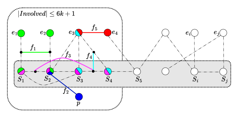
Figure 4: An example instance of Broadcast Improvement constructed by our hardness reduction, after adding $k$ edges. We use $s_{i}$ for set vertices, $e_{i}$ for element vertices, and dot-dash lines to indicate the $l$-length paths joining these. Internal vertices which are the endpoint of a new edge are shown as smaller black vertices along these paths. Among the $k$ added edges (solid), we highlight one of most types of possible edge additions as $f_{1},\ldots,f_{5}$, and indicate using the associated color the set and element vertices they involve. For clarity, several types of edge additions incident to $p$ are omitted, along with the $l$-length paths between $p$ and each set vertex. Finally, $e_{i}$ and $e_{j}$ are a pair of element vertices outside the involved set that have a distance of at least $3l$ between them. These are the vertices that we use to prove (in the no-case) that the broadcast is at most $\alpha^{3l-\varepsilon}$.

Proof.

Our reduction from Gap Set Cover is as follows

Instance: Given an instance of Gap Set Coverconsisting of a collection of $n$ sets $S_{1},S_{2},\dots,S_{n}\subseteq[m]$. We construct an Broadcast Improvement instance of $(G=(V,E,\alpha),k)$ as follows:

We create a graph $G$ with a pivot vertex $p$, vertices $s_{i}$ corresponding to sets $S_{i}$ (called set vertices) and vertices $e_{i}$ corresponding to elements $i\in[m]$ (called element vertices). Between every pair of set vertices $s_{i},s_{j}$, we add a path of length $l$, where $l$ is an even integer parameter whose value will be specified later. These paths are mutually disjoint, and so there are $\binom{n}{2}(l-1)$ vertices along the paths. We call these set-set internal vertices. Next, we add a path of length $l$ between $s_{i}$ and $e_{j}$ for all $j\in S_{i}$. (I.e., we connect a set vertex $s_{i}$ to all the element vertices $e_{j}$ corresponding to elements $j\in S_{i}$.). Once again, these paths are all mutually disjoint. We call the vertices on the paths the set-element internal vertices. Finally, we connect the pivot to each set vertex via mutually disjoint paths of length $l$. We call the internal vertices along these paths pivot-set internal vertices.

Now we argue about the maximum broadcast that can be achieved after adding $k$ edges to such a graph $G$.

Yes-case: let there be a set cover of size $k$ that covers all elements. Suppose we consider adding $k$ edges between the pivot vertex $p$ and set vertices corresponding to sets in the set cover. We claim that between any two vertices in the resulting graph, there is a path of length at most $2.5l+1$, thus implying that the broadcast $\beta({G})\geq\alpha^{2.5l+1}$.

To see the claim, we argue separately for each vertex:

First, from the pivot vertex $p$, every vertex can be reached via a path of length $\leq 2l$. To see this, note that the distance of each $e_{i}$ (and therefore also each set-element internal vertex) from $p$ is at most $l+1$; this follows because we have direct edges from $p$ to a set cover. Also, every set-vertex (and therefore also every pivot-set internal vertex) can be reached via a path of length at most $l$. Thus, all of the set-set internal vertices can be reached from $p$ via a path of length $2l$ (indeed, this can be made $1.5l$ by choosing the closer set-vertex).

Second, from any set vertex, we can reach every other set vertex using a path of length $l$, and thus every element vertex with a path of length $\leq 2l$. Further, any of the internal vertices can also be reached via a path of length $\leq 2l$, as can the pivot.

Third, from any element vertex $e_{i}$, we can reach every other element vertex $e_{j}$ with a path of length $\leq 2l+2$ (by going to the set vertex covering $i$, going to the pivot, then to the set vertex covering $j$, then going to $e_{j}$). Further, any set vertex can be reached via a path of length at most $2l$ (going to a set vertex covering $i$ and taking the length $l$ path to the desired set vertex). Any set-set internal vertex can thus be reached via a path of length at most $2.5l$: we can go from the target vertex to the closest set vertex —with a path of length $\leq 0.5l$— and from there to $e_{i}$ by a path of length $\leq 2l$ as before. Moreover, any pivot-set internal vertex can be reached via a path of length at most $2l$, using a path of length at most $l+1$ to the pivot and then proceeding to the target vertex via path of length at most $l-1$. Finally, any set-element internal vertex can be reached via a path of length $(2.5l+1)$: from the target, we can either go to an element vertex via a path of length $(0.5l-1)$ or a set vertex via a path of length $(0.5l+1)$, and using the above, this implies that we can get to the target by a path of length $2.5l+1$.

Fourth, from any pivot-set internal vertex $y$, we can reach any other pivot-set internal vertex via a path of length $<2l$ by first traveling to the pivot, and then to the target vertex. Moreover, we can reach any set-element internal vertex $x$ via a path of length at most $2.5l$. We begin by traveling to either the pivot or the set vertex corresponding to $y$ (whichever is closer) via a path of length at most $0.5l$. We then continue to $x$ via at most $2l$ additional edges, as argued above.

Next, from any set-set internal vertex, we can reach any set vertex with a path of length $\leq 1.5l$, and thus we can reach every other vertex with a path of length $\leq 2.5l$.

Finally, from a set-element internal vertex, it only remains to show that we can reach any other set-element internal vertex using a short path (other cases are covered above by symmetry). Consider two set-element internal vertices $x$ and $x^{\prime}$, with $x$ (resp., $x^{\prime}$) on the path from $s_{i}$ to $e_{j}$ (resp., $s_{i^{\prime}}$ to $e_{j^{\prime}}$). We show that there is a cycle with $5l+2$ edges in the graph that contains $x,x^{\prime}$. Note that this implies that there is a path of length $\leq 2.5l+1$ (i.e., the shorter path on the cycle). As shown in Figure 5, note that there is a path of length $2l+2$ between $e_{j}$ and $e_{j^{\prime}}$ (using the covering set vertices, as seen above), and there is also the path going to $s_{i}$, to $s_{i^{\prime}}$, then to $e_{j^{\prime}}$.

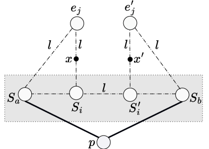
Figure 5: This figure shows the cycle of length $5l+2$ containing two set-element internal vertices $x$ and $x^{\prime}$. This cycle shows that $x$ and $x^{\prime}$ have proximity at least $\alpha^{2.5l+1}$ (in the yes-case).

This completes the proof of the claim. Thus, in the yes-case, $\beta({G})\geq\alpha^{2.5l+1}$.

No-case: By 1, the union of any $ck$ sets among $S_{1},\dots,S_{n}$ covers at most $(1-\Omega(1))m$ elements, for any constant $c\geq 1$.

Now consider adding $r=c^{\prime}k$ edges, where $r\leq ck/8$. Let $E^{\prime}$ denote the set of added edges and let $G^{\prime}$ be the graph obtained from $G$ by adding the edges in $E^{\prime}$.

For any $\{u,v\}\in E^{\prime}$, we define a set of “involved” set and element vertices as follows. A set vertex $s_{i}$ is said to be involved in edge $\{u,v\}$ if for $x\in\{u,v\}$, we have (a) $s_{i}=x$, (b) $x$ is a set-set internal vertex and one of the end-points of the corresponding path (the one containing $x$) is $s_{i}$, or (c) $x$ is a set-element internal vertex and the set end-point of the corresponding path is $s_{i}$. Analogously, we say that an element vertex $e_{i}$ is involved in edge $\{u,v\}$ if for $x\in\{u,v\}$, either (a) $e_{i}=x$ or (b) $x$ is a set-element internal vertex and $e_{i}$ is the element end-point of the corresponding path.

We also generalize the notation slightly and say that a vertex is involved in a set of edges $E^{\prime}$ if it is involved in at least one of the edges $e\in E^{\prime}$. The main claim due to our choice of parameters is the following.

Claim.

There exist element vertices $e_{i},e_{j}$ such that (a) neither of them is involved in $E^{\prime}$, (b) none of the sets containing $i,j$ are involved in $E^{\prime}$, and (c) there is no set $S_{t}$ that contains both $i$ and $j$.

Proof of Claim..

First, note that any edge $e\in E^{\prime}$ can have at most $4$ set vertices and $2$ element vertices involved in it. Thus, if we pick $r$ edges, we will have at most $4r$ set vertices and $2r$ element vertices involved. For each of the involved element vertices, choose an arbitrary set that covers that element, thus obtaining a set $I$ of $6r$ set vertices with the property that all the set and element vertices involved in $S^{\prime}$ are either in $I$ or are covered by $I$. Now by our assumption for the no-case and the choice of $r$, this means there are $\Omega(m)$ element vertices that are not covered by the sets in $I$; Call this set $U$. By definition, for any $e_{i}\in U$, none of the sets covering $e_{i}$ are in $I$ (and so property (b) automatically holds). Finally, note that there must exist $e_{i},e_{j}\in U$ such that no set vertex has length $l$ paths to both of them. This can be seen by a simple averaging argument as follows. Let $c_{ij}$ be the number of sets that contain both $i$ and $j$. Then, we have

$$\sum_{i,j\in U}c_{ij}\leq\sum_{\ell\in[n]}\binom{|S_{\ell}|}{2}\leq n\cdot\text{polylog}(n).$$

Indeed, if we take all pairs $i,j\in[m]$, the first inequality becomes equality. Now, if $c_{ij}\geq 1$ for all $i,j\in U$, then $\sum\limits_{i,j\in U}c_{ij}\geq\binom{|U|}{2}$, and since $|U|=\Omega(m)$ and $m=\Theta(n)$, this leads to a contradiction. Thus, there must exist $i,j\in U$ such that $c_{ij}=0$, and this completes the proof of part (c) of the claim. ∎

For $e_{i},e_{j}$ satisfying the claim, we show that $\mathcal{P}_{G^{\prime}}({e_{i}},{e_{j}})$ has to be small. First, note that the distance between them in $G^{\prime}$ is $\geq 3l$. This is because any path from $e_{i}$ to $e_{j}$ must go via one of the set vertices containing $i,j$, and since they are not involved in $E^{\prime}$, the shortest path between those set vertices has length $l$. Our goal now is to argue that the broadcast is also “close” to $\alpha^{3l}$. For this, we show how to simplify the graph for easier reasoning about broadcast.

Claim.

[Subset contraction] Let $S$ be any subset of the vertices of $G^{\prime}$. Define a contraction as the process where we replace $S$ with a single “hub” vertex $h$, and replace every edge of the form $\{u,v\}$ where $u\in S$ and $v\not\in S$ with $\{h,v\}$ (forming parallel edges if appropriate). Let $G^{c}$ be the graph obtained after contraction. For any $u,v\not\in S$, we have $\mathcal{P}_{G^{c}}({u},{v})\geq\mathcal{P}_{G^{\prime}}({u},{v})$.

The claim then follows immediately from the sampling-based definition of proximity: suppose we sample edges with probability $\alpha$ each, then if a path exists in $G^{\prime}$, it also exists in $G^{c}$ (because of us placing parallel paths). Now given $E^{\prime}$, define $S^{\prime}$ as the set of all set and element vertices involved in $E^{\prime}$, along with the pivot $p$. Then, define $S$ to be the union of $S^{\prime}$ and all the internal vertices along paths between vertices of $S^{\prime}$. The crucial observation now is that every edge in $E^{\prime}$ has both its end-points in $S$.

Now suppose we contract the set $S$ in $G^{\prime}$ and obtain the graph $G^{c}$. By the claim, it suffices to show an upper bound on $\mathcal{P}_{G^{c}}({e_{i}},{e_{j}})$ (where $e_{i},e_{j}$ are the element vertices that we identified earlier). To do this, we make another observation about $G^{c}$: its vertices consist of $h$ (the new hub vertex), a subset $V_{set}$ of the original set vertices, a subset $V_{elt}$ of the element vertices, all the internal vertices of the paths between $V_{set}\cup V_{elt}$, and all the internal vertices of the paths between $h$ and $V_{set}\cup V_{elt}$. Thus it is natural to define a “path compressed” graph $H$, whose vertex set is $\{h\}\cup V_{set}\cup V_{elt}$, which has an edge iff there is a path of length $l$ in $G^{c}$. Note that there can be parallel edges in $H$. Now suppose we view $H$ as an information graph, where the sampling probability is $\alpha^{l}$ for every edge. Then we have the following easy observation:

Observation 2.

For all $u,v\in\{h\}\cup V_{set}\cup V_{elt}$, we have $\mathcal{P}_{G^{c}}({u},{v})=\mathcal{P}_{H}({u},{v})$.

For our $e_{i},e_{j}$ of interest, bounding $\mathcal{P}_{H}({e_{i}},{e_{j}})$ will turn out to be simple, because the edge probability $\alpha^{l}$ will be chosen to be so small that only the shortest path between $e_{i}$ and $e_{j}$ matters. We formalize this in the following simple claim.

Claim.

Let $H=(V_{H},E_{H})$ be an information graph on $n_{H}$ vertices in which every edge has sampling probability $\leq\delta<\frac{1}{2n_{H}}$. Let $u,v\in V$ such that dist$(u,v)=c$, for some integer $c\geq 1$. Then $\mathcal{P}_{H}({u},{v})\leq 2n_{H}^{c-1}\delta^{c}$.

Proof of Claim..

For any path of length $\ell$, the probability that the path exists in a sampled graph is $\delta^{\ell}$. Between any two vertices, there are clearly at most $n_{H}^{\ell-1}$ paths of length $\ell$, and thus by a union bound, noting that dist$(u,v)=c$ and therefore there are no paths of length $<c$, we have:

$$\mathcal{P}_{H}({u},{v}) \leq\sum_{\ell=c}^{n_{H}-1}n_{H}^{\ell-1}\delta^{\ell}\leq n_{H}^{c-1}\delta^{c}\cdot\sum_{\ell\geq 0}(\delta n_{H})^{\ell}\leq 2n_{H}^{c-1}\delta^{c}.$$

∎

The claim now implies a bound on $\mathcal{P}_{H}({e_{i}},{e_{j}})$; we cannot use it directly since our $H$ has parallel edges, but we note that there are at most $6k+1$ parallel edges between any two vertices (because that is a bound on the number of “non-internal” vertices, plus the pivot, in the contracted set $S$). Thus, we can replace parallel edges by a single edge with $\delta\leq(6k+1)\alpha^{l}$, and use 2 to obtain:

$$\mathcal{P}_{H}({e_{i}},{e_{j}})=\mathcal{P}_{G^{\prime}}({e_{i}},{e_{j}})\leq\mathcal{P}_{G^{c}}({e_{i}},{e_{j}})\leq 2(m+n)^{2}\delta^{3}.$$

This is because the shortest path in $H$ between $e_{i}$ and $e_{j}$ has length three, as there is no set that contains both $i$ and $j$. Now, if we choose $l$ large enough (approximately $\frac{\log n}{\epsilon}$), we can make $2(m+n)^{2}\delta^{3}$ to be $<\alpha^{3l-\epsilon}$, for any $\epsilon>0$.

Since the broadcast in the yes-case is $\geq\alpha^{2.5l+1}$, the desired gap follows.

∎

7 Single-Source Variant

In this section we study the problem of adding edges to improve the information access of a single vertex $v_{s}$. That is, we seek to maximize the reach $\Upsilon_{G}({v_{s}})$ of $v_{s}$.

Reach Improvement
Input: An information graph $G=(V,E,\alpha)$, a vertex $v_{s}\in V$, and a non-negative integer $k$. Task: Add $k$ edges to $G$ such that the reach of $v_{s}$ in the resulting information graph is maximized.

We first show that the Broadcast Improvement algorithms which we developed in Sections 3-5 also apply in this context, with constrained loss in the guarantees.

Lemma 7.

Suppose for some functions $f,g$ a polynomial-time algorithm exists which produces broadcast at least $f(\beta^{*}{},k,\alpha)$ using $g(k)$ edge additions, given any instance of Broadcast Improvement. Then a polynomial-time algorithm exists which produces reach at least $f((\Upsilon^{*}{})^{2},k,\alpha)$ using $g(k)$ edge additions, given any instance of Reach Improvement.

Proof.

Let $G=(V,E,\alpha)$ be an information graph and $v_{s}\in V$ a source vertex. Furthermore, suppose that $\beta^{*}$ is the maximum broadcast achievable by adding $k$ edges to $G$, and that $\Upsilon^{*}$ is the maximum achievable reach of $v_{s}$ with $k$ edge additions. Suppose toward a contradiction that $\Upsilon^{*}>\sqrt{\beta^{*}}$, and let $G^{*}$ denote the information graph resulting from some optimal set of edge additions for the Reach Improvement problem. Then we have that

$$\mathcal{P}_{G^{*}}({u},{v})\geq\mathcal{P}_{G^{*}}({v_{s}},{u})\cdot\mathcal{P}_{G^{*}}({v_{s}},{v})\geq\Upsilon^{*}\cdot\Upsilon^{*}>\beta^{*}$$

Because $u$ and $v$ were chosen arbitrarily, we conclude that $\beta({G^{*}})>\beta^{*}$, a contradiction. Now that we have proven $\Upsilon^{*}\leq\sqrt{\beta^{*}}$, it is a straightforward observation that any $g(k)$ edge additions which achieve broadcast at least $f(\beta^{*},k,\alpha)$ also produce reach at least $f(\Upsilon^{*}{}^{2},k,\alpha)$ for every choice of source vertex. ∎

Paying an extra factor two in the exponent is far from desirable. Fortunately, we can use the ideas developed in Section 4 to directly obtain a multiplicative approximation for Reach Improvement using $O(k\log n)$ edges. In the following, we adapt Definition 2 to this setting in the natural way. That is, a set $W_{u}$ is a $(u,r)$-witness if $\mathcal{P}_{G+W_{u}}({v_{s}},{u})\geq r$ and a solution $S$ is $(c,r)$-witnessing if it contains as a subset a $(u,r)$-witness of size at most $c$ for every vertex $u$.

Lemma 8.

For any instance of Reach Improvement, there exists a $(1,\frac{\Upsilon^{*}{}}{2k+2})$-witnessing solution of size at most $2k$.

Proof.

Let $(G=(V,E,\alpha),v_{s},k)$ be an instance of Reach Improvement, and suppose that $S^{*}$ is an optimal solution, so $\Upsilon_{G+S^{*}}({v_{s}})=\Upsilon^{*}$. We construct an alternate solution $S$ as follows. First, impose an arbitrary ordering on the endpoints of the edges in $S$: $s_{1},s_{2},\ldots s_{m}$, and we set $S=\{v_{s}s_{1},v_{s}s_{2},\ldots v_{s}s_{m}\}$. It is clear that $S$ has size at most $2k$, so what remains is to prove that $S$ contains a $(u,\frac{\Upsilon^{*}}{2k+2})$-witness of size at most 1 for every $u\in V$.

Let $P_{v_{s}u}$ be all paths from $v_{s}$ to $u$ in $G+S^{*}$. We partition these paths according to the last edge in $S^{*}$ to appear along the path. This creates at most $k+1$ equivalence classes, including the class of paths which already existed in $G$ before any edge additions were made. The sum of the contributions of each equivalence class is an upper bound for $\mathcal{P}_{G+S^{*}}({v_{s}},{u})$, and therefore also for $\Upsilon^{*}$. Then there is at least one equivalence class with contribution at least $\Upsilon^{*}/(k+1)$. If one such class is the set of paths using no edges from $S^{*}$, then the empty set is our witness. Otherwise, let $P_{v_{s}u}^{ij}$ be such an equivalence class, corresponding to edge $s_{i}s_{j}\in S^{*}$. We further partition this set of paths according to which of $s_{i}$ or $s_{j}$ is the trailing vertex of $s_{i}s_{j}$ in a given path. One of these subsets has contribution at least half of that of $P_{v_{s}u}^{ij}$, i.e., at least $\Upsilon^{*}/(2k+2)$. Call this subset $\mathcal{C}$, and assume without loss of generality that it is the subset corresponding to vertex $s_{i}$.

We now show how to replace $\mathcal{C}$ with a new set of paths $Q$ which has contribution at least $\Upsilon^{*}/(2k+2)$ and which contains only one edge, specifically $v_{s}s_{i}$, from $S$. This completes the proof, as it shows that $\{v_{s}s_{i}\}$ is a $(u,\frac{\Upsilon^{*}}{2k+2})$-witness of size 1. For each path $p\in\mathcal{C}$, we replace $p[v_{s},s_{i}]$ with the edge $v_{s}s_{i}$. By construction, $v_{s}s_{i}$ is the only edge from $S$ contained in any path in $Q$. Moreover, we note that $Q[s_{i},u]=\mathcal{C}[s_{i},u]$. Let $\mathcal{E}_{1}$ be the event that a path from one of these segments is sampled. We note that for a path in $\mathcal{C}$ to be sampled, we require both event $\mathcal{E}_{1}$ and that the edge $s_{j}s_{i}$, which appears on no path in $\mathcal{C}[s_{i},u]$, is sampled. Thus, we have $\Pr[\mathcal{C}]\leq\alpha\Pr[\mathcal{E}_{1}]$. Meanwhile, $\Pr[Q]=\alpha\Pr[\mathcal{E}_{1}]$, as the paths in $Q[s_{1},u]$ and the edge $v_{s}s_{i}$ are sampled independently. The result follows.

∎

We now show how to use $O(k\log n)$ edges to obtain a guarantee of either $\frac{\Upsilon^{*}}{(1+\varepsilon)(2k+2)}$ or $\frac{\Upsilon^{*}\alpha}{(1+\varepsilon)(1+2k\alpha)}$. Both algorithms work via reductions to Hitting Set, with the former guarantee relying on Lemma 8 and the latter on Lemma 1. The former guarantee is stronger if $\alpha<\frac{1}{2}$ and the latter is stronger if $\alpha>\frac{1}{2}$. Similarly to Theorem 4, we also use the reductions to Hitting Set to conduct a binary search until we have found a good estimate for the value of $\Upsilon^{*}$.

Theorem 8.

Given any $\alpha,\varepsilon>0$, there exists a polynomial-time algorithm which produces reach (for a given source vertex $v_{s}$) at least $\max\{\frac{\Upsilon^{*}}{(1+\varepsilon)(2k+2)},\frac{\Upsilon^{*}\alpha}{(1+\varepsilon)(1+2k\alpha)}\}$ using $O(k\log n)$ edge additions.

Proof.

Let $(G=(V,E,\alpha),v_{s},k)$ be an instance of Reach Improvement. We begin by assuming that we already know the optimum achievable reach $\Upsilon^{*}$. We reduce to Hitting Set. If $\alpha\leq\frac{1}{2}$, then the reduction proceeds as follows. The elements of our Hitting Set instance are $V^{2}\setminus E$, i.e., all possible edge additions. For each vertex $u\in V$ with $\mathcal{P}_{G}({v_{s}},{u})<\Upsilon^{*}$, we create a set $\mathcal{W}_{u}$ consisting of all single edge-additions which improve the proximity of $v_{s}$ to $u$ to at least $\frac{\Upsilon^{*}}{2k+2}$. That is, $\mathcal{W}_{u}$ is the set of all $(u,\frac{\Upsilon^{*}}{2k+2})$-witnesses of size 1. According to Lemma 8, there exists a hitting set of size at most $2k$. We use the well-known greedy approximation for Hitting Set [23] to obtain a hitting set of size $O(k\log n)$, and we return these edges as our solution. It follows from the construction that this solution achieves reach at least $\frac{\Upsilon^{*}}{2k+2}$.

On the other hand, if $\alpha>\frac{1}{2}$, then we reduce to Hitting Set as follows. Our elements are $V\setminus v_{s}$, i.e., all vertices except the source. For each vertex $u\neq v_{s}$, we add a set equal to the $\frac{\Upsilon^{*}}{1+2k\alpha}$-neighborhood of $u$. We claim that there exists a hitting set of size at most $2k$. Otherwise, for any optimal solution $S^{*}$ which adds $k$ edges, there exists some vertex $u\neq v_{s}$ such that the endpoints of these edges are disjoint from the $\frac{\Upsilon^{*}}{1+2k\alpha}$-neighborhood of $u$. But then Lemma 1 gives us that $\mathcal{P}_{G+S^{*}}({u},{v_{s}})<\Upsilon^{*}$, a contradiction. Hence, we can once again use the greedy approximation for Hitting Set to obtain a set of $O(k\log n)$ vertices. We add the edges between these vertices and $v_{s}$, guaranteeing reach at least $\frac{\Upsilon^{*}\alpha}{1+2k\alpha}$ as desired.

It remains to show how we can estimate $\Upsilon^{*}$. In the following, let $b$ be the precise bound on edge additions given by the algorithm described above. That is, $b$ is $2k$ multiplied by the precise factor given by the algorithm in [23]. We note that $\Upsilon_{G}({v_{s}})\leq\Upsilon^{*}\leq 1$, so there exists an integer $0\leq i\leq\log_{i+\varepsilon}\frac{1}{\Upsilon_{G}({v_{s}})}$ such that $\Upsilon_{G}({v_{s}})(1+\varepsilon)^{i}\leq\Upsilon^{*}\leq\Upsilon_{G}({v_{s}})(1+\varepsilon)^{i+1}$. We conduct a binary search of integers in the interval $[0,\log_{i+\varepsilon}\frac{1}{\Upsilon_{G}({v_{s}})}]$. For each tested value $j$, we assume that $\Upsilon^{*}=\Upsilon_{G}({v_{s}})(1+\varepsilon)^{j}$ and run the algorithm described above. If the resulting set of edge additions has size greater than $b$, then we use Lemma 8 to conclude that $j>i$. Now, let $j^{*}$ be the largest integer in the interval for which the algorithm adds at most $b$ edges. Then we can conclude that $\Upsilon^{*}\leq\Upsilon_{G}({v_{s}})(1+\varepsilon)^{j^{*}+1}$, and the algorithm gives us a set of at most $b\in O(k\log n)$ edge additions which achieve reach at least

$$\frac{\Upsilon_{G}({v_{s}})(1+\varepsilon)^{j^{*}}}{2k+2}=\frac{\Upsilon_{G}({v_{s}})(1+\varepsilon)^{j^{*}+1}}{(1+\varepsilon)(2k+2)}\geq\frac{\Upsilon^{*}}{(1+\varepsilon)(2k+2)}.$$

So we have successfully computed the desired approximation. ∎

We conclude this section by showing that no polynomial time algorithm using $O(k)$ edge additions can achieve a multiplicative approximation for Reach Improvement, unless P = NP.

Theorem 9.

For any $\varepsilon,\alpha>0$ and any constant $c\geq 1$, it is NP-hard to provide reach at least $\big{(}\Upsilon^{*})^{\frac{4}{3}-\varepsilon}$ using $ck$ edge additions.

Proof.

We once again reduce from Gap Set Cover. Let $(S_{1},S_{2},\ldots S_{n}\subseteq[m],k)$ be an instance of this problem. Recall that it is NP-hard to distinguish between the cases (i) there exists a collection of at most $k$ sets which cover every element, and (ii) any collection of $2ck$ sets leaves at least $2ck+1$ elements uncovered [12, 14, 13]. Let $d$ be the maximum size of any set, i.e., $d=\max_{i\in[n]}|S_{i}|$. Let $b$ be the maximum number of sets containing any single element, i.e., $b=\max_{j\in[m]}|\{i\in[n]\colon j\in S_{i}\}|$. Finally, we will need an additional value $l$, which can be thought of as an integer which is polynomial in $m+n$. We will show how to select the exact value of $l$ at the end of the proof.

We construct an instance of Reach Improvement as follows. First we introduce a vertex $v_{s}$, which will be the source vertex of our constructed instance. Next, for each set $S_{i}$, $i\in[n]$, we introduce a vertex $v_{i}$. We call these vertices set vertices. For each set vertex $v_{i}$, we introduce $l-1$ auxiliary vertices and $l$ edges, such that $v_{i}$ is connected to $v_{s}$ by a path of edge-length $l$ on these vertices and edges. We call these auxiliary vertices the set-path vertices corresponding to set $S_{i}$. So far, we have added (less than) $1+ln$ vertices and exactly $ln$ edges. Next, for each element $j\in[m]$, we add a new vertex $v_{j}$, which we call an element vertex. For each set $S_{i}$ containing element $j$, we add $l-1$ auxiliary vertices and $l$ edges such that $v_{i}$ and $v_{j}$ are connected by a path of edge-length $l$ on these vertices and edges. We call these auxiliary vertices the set-element-path vertices corresponding to set $S_{i}$ and element $j$. This step adds at most $m\cdot d\cdot l$ vertices and edges. We call the information graph we have constructed $G$. We set the limit on edge additions to $k$, and the target value for the reach of $v_{s}$ to $\alpha^{\frac{3l}{2}+1}$. This completes the construction of our instance of Reach Improvement.

It remains to show that the reduction is correct. We begin by assuming that $(\{S_{i}\}_{i\in[n]},k)$ is a yes-instance. That is, we assume that there exist $k$ sets $S_{i_{1}},S_{i_{2}},\ldots,S_{i_{k}}$ which cover every element. In this case, we add the $k$ edges between $v_{s}$ and the set vertices corresponding to this set cover. That is, we propose the solution $S=\{v_{s}v_{i_{1}},v_{s}v_{i_{2}},\ldots,v_{s}v_{i_{k}}\}$. Now we show that $\Upsilon_{G+S}({v_{s}})\geq\alpha^{\frac{3l}{2}+1}$. Let $u\neq v_{s}$ be some vertex in $G$. If $u$ is a set vertex or a set-path vertex, then our initial construction guarantees that $\mathcal{P}_{G+S}({u},{v_{s}})\geq\mathcal{P}_{G}({u},{v_{s}})\geq\alpha^{l}$. If $u$ is an element vertex, then we identify a set $S_{i}$ which contains the element corresponding to $u$ and is part of the cover. Then

$$\mathcal{P}_{G+S}({u},{v_{s}})\geq\mathcal{P}_{G+S}({u},{S_{i}})\cdot\mathcal{P}_{G+S}({S_{i}},{v_{s}})\geq\alpha^{l}\cdot\alpha=\alpha^{l+1}$$

Finally, assume that $u$ is a set-element-path vertex corresponding to set $S_{i}$ and element $j$. Observe that either $\mathcal{P}_{G}({u},{v_{i}})\geq\alpha^{\frac{l}{2}}$ or $\mathcal{P}_{G}({u},{v_{j}})\geq\alpha^{\frac{l}{2}}$. In the former case,

$$\mathcal{P}_{G+S}({u},{v_{s}})\geq\alpha^{\frac{l}{2}}\cdot\mathcal{P}_{G+S}({v_{i}},{v_{s}})\geq\alpha^{\frac{3l}{2}}$$

and in the latter case

$$\mathcal{P}_{G+S}({u},{v_{s}})\geq\alpha^{\frac{l}{2}}\cdot\mathcal{P}_{G+S}({v_{j}},{v_{s}})\geq\alpha^{\frac{3l}{2}+1}$$

Thus, all vertices have proximity at least $\alpha^{\frac{3l}{2}+1}$ to $v_{s}$ in $G+S$, so $S$ witnesses that $(G,v_{s},k,\alpha^{\frac{3l}{2}+1})$ is a yes-instance of Reach Improvement.

We now assume that $(\{S_{i}\}_{i\in[n]},k)$ is a no-instance of Gap Set Cover. In this case, we let $S^{*}$ be an optimal solution to our constructed instance of Reach Improvement, and additionally allow that $S^{*}$ may contain up to $ck$ edges. That is, $S^{*}$ is a set of at most $ck$ edge additions, with $\Upsilon_{G+S^{*}}({v_{s}})\geq\Upsilon^{*}$. We will first give an upper bound on $\Upsilon^{*}$, and then show how we could have chosen $l$ such that this upper bound yields the desired hardness result. We impose an arbitrary order on the (at most $2ck$) endpoints of the edges in $S^{*}$, $s_{1},s_{2},\ldots s_{ck}$. We then introduce a new solution $S$ of size at most $2ck$ such that $S=\{v_{s}s_{1},v_{s}s_{2},\ldots,v_{s}s_{2ck}\}$. By carefully inspecting the proof of Lemma 8, we observe that $\Upsilon_{G+S}({v_{s}})\geq\frac{\Upsilon^{*}}{2ck+2}$. We call the vertices $s_{1},s_{2},\ldots s_{2ck}$ the destinations of the solution $S$, and we say that a set $S_{i}$ is involved in solution $S$ if the destinations of $S$ include the set vertex $v_{i}$, any set-path vertex corresponding to $S_{i}$, or any set-element-path vertex corresponding to $S_{i}$. Note that every set-path vertex and every set-element-path vertex corresponds to exactly one set, so since $S$ has at most $2ck$ destinations we can conclude that at most $2ck$ sets are involved in $S$. Next, we say that an element $j$ is uncovered if it is not contained in any set which is involved in $S$. Because only $2ck$ sets are involved in $S$, at least $2ck+1$ elements are uncovered. Moreover, because $S$ has at most $2ck$ destinations, there is at least one uncovered element $j$ for which the corresponding element vertex $v_{j}$ is not itself a destination of $S$. We will now show that $\mathcal{P}_{G+S}({v_{j}},{v_{s}})\leq\alpha^{2l}(b+bd)$.

Every path from $v_{j}$ to $v_{s}$ begins with $l$ edges from $v_{j}$ to some set vertex $v_{i}$, where $j\in S_{i}$ and $S_{i}$ is not involved in $S$. From there, paths extend either via $l$ more edges to $v_{s}$, or via $l$ more edges to another element vertex. Each path of the former variety has contribution $\alpha^{2l}$, and $j$ is contained in at most $b$ sets, so these paths have contribution at most $b\alpha^{2l}$. Similarly, there are at most $bd$ paths of the latter variety, and each has contribution $\alpha^{2l}$. Hence,

$$\Upsilon^{*}\leq\Upsilon_{G+S}({v_{s}})(2k+2)\leq\mathcal{P}_{G+S}({v_{j}},{v_{s}})(2k+2)\leq\alpha^{2l}(b+bd)(2ck+2)$$

We now claim that to achieve the desired hardness bound we need only set

$$l>\frac{2}{3\varepsilon}\big{[}-\log_{\alpha}(b+bd)-\log_{\alpha}(2ck+2)+\frac{4}{3}-\varepsilon\big{]}$$

In this case, simple manipulations reveal that

$$\frac{3\varepsilon l}{2} >-\log_{\alpha}(b+bd)-\log_{\alpha}(2ck+2)+\frac{4}{3}-\varepsilon$$

$$\alpha^{\frac{3\varepsilon l}{2}}(b+bd)(2ck+2) <\alpha^{\frac{4}{3}}\alpha^{-\varepsilon}$$

$$\alpha^{2l}\alpha^{\frac{3\varepsilon l}{2}}(b+bd)(2ck+2) <\alpha^{2l}\alpha^{\frac{4}{3}}\alpha^{-\varepsilon}$$

$$\alpha^{2l}(b+bd)(2ck+2) <\alpha^{2l}\alpha^{\frac{-3\varepsilon l}{2}}\alpha^{\frac{4}{3}}\alpha^{-\varepsilon}$$

$$\Upsilon^{*} <(\alpha^{\frac{3l}{2}+1})^{\frac{4}{3}-\varepsilon}$$

Consequently, any algorithm which produces reach at least $(\Upsilon^{*})^{\frac{4}{3}-\varepsilon}$ using at most $ck$ edges can also distinguish between yes- and no-instances of Gap Set Cover. This completes the proof. ∎

8 Conclusion

We have studied the problem of adding edges to a network to optimize the broadcast of that network, where broadcast is defined as the minimum pairwise access under the Independent Cascade model of information propagation. This work extends the contributions of [2] by providing the first formal approximation guarantees for Broadcast Improvement. We provide algorithms with varying trade-offs using three broad techniques.

Next, we prove the hardness of Broadcast Improvement by showing that no algorithm adding $O(k)$ edges can guarantee broadcast at least $(\beta^{*})^{6/5-\varepsilon}$, unless P = NP. Finally, we examine the single-source variant of the problem, in which the goal is to maximize the information access of a single vertex. We show that algorithms for Broadcast Improvement extend to Reach Improvement, with bounded loss in the objective value. We also give a direct algorithm which achieves a reach value linear in $\Upsilon^{*}$, adding only $O(k\log n)$ edges, and show that it is NP-hard to guarantee reach at least $(\Upsilon^{*})^{4/3-\varepsilon}$ with $O(k)$ edge additions.

Interesting questions remain. First, we ask if bicriteria approximation is necessary at all: does there exist an efficient algorithm which adds exactly $k$ edges and obtains a broadcast value $(\beta^{*})^{O(1)}$? Regarding our “constant witness” technique, it would be interesting to determine whether algorithms using $O(k\log n)$ edges can be obtained without using submodularity. In particular, we ask whether the following generalization of Hitting Set admits a $O(\log m)$-approximation.

$c$-Bounded-Combination Hitting Set
Input: $n$ sets over combinations of $m$ elements: $S_{1},S_{2},\ldots,S_{n}\subseteq\binom{[m]}{c}$. Task: Find a subset of elements $E\subseteq[m]$ of minimum size such that for each $i\in[n]$, some element of $S_{i}$ is a subset of $E$.

Such an algorithm would allow us to immediately improve the bounds on edge additions given in Theorem 4 to $O(k\log n)$, and would broaden the applicability of the constant witness technique.

We also ask whether the techniques developed in Section 5 can be extended to address part (i) of Theorem 4. In this case, a starting point is to approximate via submodularity a somewhat more complicated structure: a tri-centered star on $2k$ leaves. Finally, it remains open to provide algorithms with provable guarantees for Broadcast Improvement and Reach Improvement for non-uniform values of the edge propagation probability $\alpha$.

More broadly, we suggest that studying algorithmic approaches to network design under stochastic models of information flow is a rich and relatively unexplored direction for future research. Possible directions include the optimization of other metrics, e.g., the access centrality defined by [2], and the consideration of other propagation models, e.g., linear threshold [18].

References

- Ali et al. [2019] J. Ali, M. Babaei, A. Chakraborty, B. Mirzasoleiman, K. P. Gummadi, and A. Singla. On the fairness of time-critical influence maximization in social networks, 2019.
- Bashardoust et al. [2023] A. Bashardoust, S. Friedler, C. Scheidegger, B. D. Sullivan, and S. Venkatasubramanian. Reducing access disparities in networks using edge augmentation. In Proceedings of the 2023 ACM Conference on Fairness, Accountability, and Transparency, FAccT ’23, pages 1635–1651. Association for Computing Machinery, 2023.
- Becker et al. [2021] R. Becker, G. D’Angelo, S. Ghobadi, and H. Gilbert. Fairness in influence maximization through randomization. Proceedings of the AAAI Conference on Artificial Intelligence, 35(17):14684–14692, May 2021. URL https://ojs.aaai.org/index.php/AAAI/article/view/17725.
- Becker et al. [2023] R. Becker, G. D’Angelo, and S. Ghobadi. Improving fairness in information exposure by adding links, 2023.
- Beilinson et al. [2020] H. C. Beilinson, N. Ulzii-Orshikh, A. Bashardoust, S. A. Friedler, C. E. Scheidegger, and S. Venkatasubramanian. Clustering via information access in a network. arXiv, abs/2010.12611, 2020.
- Bergamini et al. [2018] E. Bergamini, P. Crescenzi, G. D’angelo, H. Meyerhenke, L. Severini, and Y. Velaj. Improving the betweenness centrality of a node by adding links. Journal of Experimental Algorithmics (JEA), 23:1–32, 2018.
- Bilò et al. [2012] D. Bilò, L. Gualà, and G. Proietti. Improved approximability and non-approximability results for graph diameter decreasing problems. Theoretical Computer Science, 417:12–22, 2012.
- Chen et al. [2010] W. Chen, C. Wang, and Y. Wang. Scalable influence maximization for prevalent viral marketing in large-scale social networks. In B. Rao, B. Krishnapuram, A. Tomkins, and Q. Yang, editors, Proceedings of the 16th ACM SIGKDD International Conference on Knowledge Discovery and Data Mining, Washington, DC, USA, July 25-28, 2010, pages 1029–1038. ACM, 2010. doi: 10.1145/1835804.1835934. URL https://doi.org/10.1145/1835804.1835934.
- Crescenzi et al. [2016] P. Crescenzi, G. D’angelo, L. Severini, and Y. Velaj. Greedily improving our own closeness centrality in a network. ACM Transactions on Knowledge Discovery from Data (TKDD), 11(1):1–32, 2016.
- Crespelle et al. [2023] C. Crespelle, P. G. Drange, F. V. Fomin, and P. Golovach. A survey of parameterized algorithms and the complexity of edge modification. Computer Science Review, 48:100556, 2023. ISSN 1574-0137. doi: https://doi.org/10.1016/j.cosrev.2023.100556. URL https://www.sciencedirect.com/science/article/pii/S1574013723000230.
- Demaine and Zadimoghaddam [2010] E. D. Demaine and M. Zadimoghaddam. Minimizing the diameter of a network using shortcut edges. In H. Kaplan, editor, Algorithm Theory - SWAT 2010, 12th Scandinavian Symposium and Workshops on Algorithm Theory, Bergen, Norway, June 21-23, 2010. Proceedings, volume 6139 of Lecture Notes in Computer Science, pages 420–431. Springer, 2010. doi: 10.1007/978-3-642-13731-0\_39. URL https://doi.org/10.1007/978-3-642-13731-0_39.
- Feige [1998] U. Feige. A threshold of ln n for approximating set cover. J. ACM, 45(4):634–652, jul 1998. ISSN 0004-5411. doi: 10.1145/285055.285059. URL https://doi.org/10.1145/285055.285059.
- Feige and Vondrák [2010] U. Feige and J. Vondrák. The submodular welfare problem with demand queries. Theory of Computing, 6(11):247–290, 2010. doi: 10.4086/toc.2010.v006a011. URL https://theoryofcomputing.org/articles/v006a011.
- Feige et al. [2004] U. Feige, L. Lovász, and P. Tetali. Approximating min sum set cover. Algorithmica, 40:219–234, 2004.
- Feldmann and Marx [2020] A. E. Feldmann and D. Marx. The parameterized hardness of the k-center problem in transportation networks. Algorithmica, 82:1989–2005, 2020.
- Fish et al. [2019] B. Fish, A. Bashardoust, d. boyd, S. Friedler, C. Scheidegger, and S. Venkatasubramanian. Gaps in information access in social networks. In WWW, pages 480–490, 2019.
- Gonzalez [1985] T. F. Gonzalez. Clustering to minimize the maximum intercluster distance. Theoretical computer science, 38:293–306, 1985.
- Granovetter and Soong [1983] M. Granovetter and R. Soong. Threshold models of diffusion and collective behavior. Journal of Mathematical sociology, 9(3):165–179, 1983.
- Hochbaum and Shmoys [1985] D. S. Hochbaum and D. B. Shmoys. A best possible heuristic for the k-center problem. Mathematics of operations research, 10(2):180–184, 1985.
- Hochbaum and Shmoys [1986] D. S. Hochbaum and D. B. Shmoys. A unified approach to approximation algorithms for bottleneck problems. Journal of the ACM (JACM), 33(3):533–550, 1986.
- Jalali et al. [2020] Z. S. Jalali, W. Wang, M. Kim, H. Raghavan, and S. Soundarajan. On the information unfairness of social networks. In Proceedings of the 2020 SIAM International Conference on Data Mining, pages 613–521. SIAM, 2020.
- Jalali et al. [2022] Z. S. Jalali, Q. Chen, S. M. Srikanta, W. Wang, M. Kim, H. Raghavan, and S. Soundarajan. Fairness of information flow in social networks. ACM Transactions on Knowledge Discovery from Data, 2022.
- Johnson [1974] D. S. Johnson. Approximation algorithms for combinatorial problems. Journal of Computer and System Sciences, 9(3):256–278, 1974.
- Kempe et al. [2003] D. Kempe, J. M. Kleinberg, and É. Tardos. Maximizing the spread of influence through a social network. In KDD, pages 137–146, 2003.
- Mehrotra et al. [2022] A. Mehrotra, J. Sachs, and L. E. Celis. Revisiting group fairness metrics: The effect of networks. Proceedings of the ACM on Human-Computer Interaction, 6(CSCW2):1–29, 2022.
- Papagelis et al. [2011] M. Papagelis, F. Bonchi, and A. Gionis. Suggesting ghost edges for a smaller world. In Proceedings of the 20th ACM international conference on Information and knowledge management, pages 2305–2308, 2011.
- Rahmattalabi et al. [2021] A. Rahmattalabi, S. Jabbari, H. Lakkaraju, P. Vayanos, M. Izenberg, R. Brown, E. Rice, and M. Tambe. Fair influence maximization: A welfare optimization approach. Proceedings of the AAAI Conference on Artificial Intelligence, 2021.
- Stoica and Chaintreau [2019] A.-A. Stoica and A. Chaintreau. Fairness in social influence maximization. In WWW, pages 569–574, 2019.
- Swift et al. [2022] I. P. Swift, S. Ebrahimi, A. Nova, and A. Asudeh. Maximizing fair content spread via edge suggestion in social networks. Proc. VLDB Endow., 15(11):2692–2705, sep 2022.
- Tsang et al. [2019] A. Tsang, B. Wilder, E. Rice, M. Tambe, and Y. Zick. Group-fairness in influence maximization. In Proc. of the Int’l Joint Conf. on Artificial Intelligence, pages 5997–6005. AAAI Press, 2019.