Open quantum dynamics with variational non-Gaussian states and the truncated Wigner approximation

Abstract

We present a framework for simulating the open dynamics of spin-boson systems by combing variational non-Gaussian states with a quantum trajectories approach. We apply this method to a generic spin-boson Hamiltonian that has both Tavis-Cummings and Holstein type couplings, and which has broad applications to a variety of quantum simulation platforms, polaritonic physics, and quantum chemistry. Additionally, we discuss how the recently developed truncated Wigner approximation for open quantum systems can be applied to the same Hamiltonian. We benchmark the performance of both methods and identify the regimes where each method is best suited to. Finally we discuss strategies to improve each technique.

I Introduction

Advances in the control of quantum systems over the past decade have led to the development of a wide variety of different platforms for investigating almost-coherent quantum dynamics. However, in the absence of robust fault-tolerant operations, studies of these platforms must contend with various sources of noise induced by couplings to an environment. Moreover, these noisy intermediate-scale quantum (NISQ Preskill (2018)) devices can often be arbitrarily controlled, opening possibilities of creating states far out of equilibrium. In light of this, understanding the out-of-equilibrium dynamics of open quantum many-body systems has become of great interest, e.g. for understanding and realizing a quantum advantage in the NISQ era.

A particularly challenging class of problems arises for systems containing both spin and bosonic degrees of freedom with an (even locally) unbounded Hilbert space, applicable to quantum simulation and computation platforms ranging from superconducting circuits to trapped ions Peropadre et al. (2013); Yoshihara et al. (2017); Forn-Díaz et al. (2017); Magazzù et al. (2018); Marcuzzi et al. (2017); Gambetta et al. (2020); Tamura et al. (2020); Skannrup et al. (2020); Méhaignerie et al. (2023); James (2000); Porras and Cirac (2004); Schneider et al. (2012); Kienzler et al. (2015); Lo et al. (2015); Kienzler et al. (2017), to paradigmatic problems in impurity physics Pérez-Ríos (2021); Lous and Gerritsma (2022), quantum chemistry Valahu et al. (2023), or polaritonic chemistry Garcia-Vidal et al. (2021). The ubiquity and complexity of spin-boson Hamiltonians has led to the development of various techniques for their study and characterization. These include methods for the bosonic space, namely path integral techniques Nalbach and Thorwart (2010); Kast and Ankerhold (2013); Nalbach and Thorwart (2013); Otterpohl et al. (2022), effective Hamiltonian formulation Lee et al. (2001); Rychkov and Vitale (2015); Szász-Schagrin and Takács (2022); Rakovszky et al. (2016) or lightcone conformal truncation used predominantly in high-energy physics Anand et al. (2020); Chen et al. (2022); Delacrétaz et al. (2023), as well as methods such as non-equilibrium Monte Carlo or tensor networks del Pino et al. (2018); Wellnitz et al. (2022); Wall et al. (2016), which have allowed for the simulation of (open) out-of-equilibrium dynamics of quantum many-body systems Makri and Makarov (1995); Thorwart et al. (1998, 2000); Schmidt et al. (2008); Schollwöck (2011); Orús (2014); Montangero (2018); White and Feiguin (2004); Schmitteckert (2004); Nuss et al. (2015); Dóra et al. (2017); Zwolak and Vidal (2004); Daley (2014); Preisser et al. (2023), also in large-system scenarios. However, these methods are often constrained to one-dimensional setups, closed systems, or to a mesoscopic number of particles, or a combination thereof.

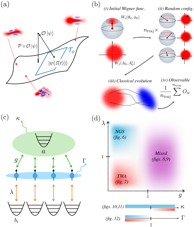
Figure 1: (a) Schematic overview of NGS. The ansatz $\ket{\psi(\vec{z}(t)}$ is a point in a manifold embedded in Hilbert space. For different variational parameters, we can describe a variety of quantum states (some example Wigner functions are shown). The action of an operator $\mathcal{O}$, which can be a Hamiltonian $H$, non-Hermitian Hamiltonian $H_{\text{eff}}$, or quantum jump $c$, can cause the state to leave the the variational manifold, so the state is projected back to the manifold $\mathcal{P}\ket{\psi}$. (b) Schematic depiction of TWA. $(i)$ The initial quantum state of the spin and bosonic degrees of freedom can be represented by the spin Wigner functions $W_{i}(\theta_{0},\phi_{0})$ and bosonic Wigner functions $W_{j}(A_{0},A_{0}^{*})$, respectively. $(ii)$ Classical phase space points are individually sampled from the initial Wigner functions for each degree of freedom and $(iii)$ evolve according to the classical (stochastic) equations of motion. $(iv)$ Expectation values of observables are evaluated in phase space by computing the average of the associated Weyl symbols over $n_{\rm traj}$ phase space trajectories. (c) Both NGS and TWA apply to generic spin-boson systems, but we depict here the system studied in this work: $N_{s}$ spins-$1/2$ interact with a common mode $a$ with strength $g$ and particle loss at rate $\kappa$. Each spin also interacts with a mode $b$ at strength $\lambda$. The spins also undergo collective loss at rate $\Gamma$. (d) Schematic summary of our results illustrating the regions where each method tends to perform well together with the reference to figures studying the dynamics in the respective parameter regimes, see Fig. 5 and Sec. V for more details.

The number and breadth of the aforementioned approaches illustrates that no single method can tackle the range of systems described by spin-boson type Hamiltonians or even the full parameter space of a specific model. As such, it is important to pinpoint the strengths and shortcomings of each method. In this work, we undertake a comparative study between two methods: (i) the time-dependent variational ansatz using non-Gaussian states (NGS) Shi et al. (2018); Hackl et al. (2020) and (ii) the truncated Wigner approximation (TWA) combined with its generalization to discrete spaces, discrete truncated Wigner approximation (DTWA). Fig. 1(a),(b) shows a schematic of each method. These methods may allow us to circumvent some of the aforementioned limitations Shi et al. (2018); Hackl et al. (2020); Schachenmayer et al. (2015a); Piñeiro Orioli et al. (2017); Zhu et al. (2019) and have recently been generalized to open quantum systems Joubert-Doriol and Izmaylov (2015); Schlegel et al. (2023); Huber et al. (2021, 2022); Singh and Weimer (2022); Mink et al. (2022); Mink and Fleischhauer (2023). Analyzing fundamental quantum effects in macroscopic limits can thus be enabled with NGS and TWA approaches.

In NGS, one exploits the continuous variable structure of bosonic states to build a time-dependent variational wavefunction ansatz of non-Gaussian states. Here, we specifically use a superposition of squeezed displaced bosonic states, which converges to the true wavefunction due to the over-completeness of the set of coherent states. Since each state in the superposition is Gaussian, much of the previously developed machinery for Gaussian states can be re-utilized. This method has been successfully applied to studies of systems ranging from the Kondo impurity problem Ashida et al. (2019a), central spin Ashida et al. (2019b), spin-Holstein models Knörzer et al. (2022), Bose and Fermi polarons Christianen et al. (2022a, b); Dolgirev et al. (2021), and (sub/super) Ohmic spin-boson model Bond et al. (2024). We also note that the closely related Davydov state ansatz has been applied in the studies of molecular crystals and polaritonic physics Chen et al. (2023); Zhao (2023); Sun et al. (2022); Zhou et al. (2015, 2014); Wu et al. (2013).

TWA is a semi-classical approach that factorizes the phase space functions (Weyl symbols) that describe a quantum observable in the phase space representation. As such, TWA is reminiscent of a product-state mean-field ansatz on Hilbert space. Like the latter, TWA allows one to treat systems with very large sizes [$\order{10^{4}}$ particles], while still capturing some essential quantum features such as spin-squeezing or entanglement Schachenmayer et al. (2015a); Lepoutre et al. (2019); Perlin et al. (2020); Franke et al. (2023); Muleady et al. (2023); Young et al. (2024). TWA can be easily adapted to systems with both bosonic and discrete degrees of freedom, combining sampling strategies from continuous Polkovnikov (2010a) and discrete Wigner functions Schachenmayer et al. (2015a); Zhu et al. (2019); Piñeiro Orioli et al. (2017).

Here, we consider the open and closed dynamics of a spin-boson Hamiltonian featuring multiple spins coupled to a discrete set of bosonic modes via Holstein and Tavis-Cummings couplings, thus ensuring broad applicability of our results. We begin by introducing the two methods: the NGS method using our multi-polaron formulation introduced in Ref. Bond et al. (2024) is discussed in Sec. II. We extend the method to open quantum systems using the quantum trajectories method in Sec. III. We discuss TWA with its discrete variant DTWA for closed and open systems in Sec. IV. In Sec. V we introduce the Holstein-Tavis-Cummings spin-boson Hamiltonian, which we use to compare both methods over a range of parameters. Finally in Sec. VI we summarize our findings and discuss how each method can be improved to increase its accuracy and/or applicability both in terms of systems to which they can be applied, and also in terms of the observables that can be accessed.

II Non-Gaussian ansatz for a closed system

We begin by introducing the non-Gaussian ansatz, before discussing how to compute the equations of motion (EOMs) for the variational parameters. We consider a system of $N_{s}$ spins-1/2 and $N_{b}$ bosonic modes governed by some Hamiltonian $H(t)$. Our wavefunction, $\ket{\psi(\vec{z})}$, is a variational ansatz in the form of a non-Gaussian state parameterized by a set of real numbers $\vec{z}$,

$$\ket{\psi(\vec{z})}=\sum_{\sigma=1}^{2^{N_{s}}}\sum_{p=1}^{N_{p}}{U}_{p}^{(\sigma)}\ket{\sigma,0},$$ (1)

where the summation over $\sigma$ is over all $2^{N_{s}}$ spin basis states . The summation over $p$ produces a superposition of $N_{p}$ bosonic states $U_{p}^{(\sigma)}\ket{0}$ for each spin degree of freedom. Following Ref. Bond et al. (2024) we refer to these states as polarons, and choose the operator $U_{p}^{(\sigma)}$ to be of the form of a Gaussian unitary,

$${U}_{p}^{(\sigma)}=e^{\kappa_{p}^{(\sigma)}+i\theta_{p}^{(\sigma)}}\mathcal{D}(\vec{\alpha}_{p}^{(\sigma)})\mathcal{S}(\vec{\zeta}_{p}^{(\sigma)}).$$ (2)

The parameters $\kappa_{p}$ and $\theta_{p}$ determine the weight and phase factors, while the many-mode displacement $\mathcal{D}(\vec{\alpha})$ and squeezing $\mathcal{S}(\vec{\zeta})$ operators are defined as,

$$\mathcal{D}(\vec{\alpha}) =\prod_{k=1}^{N_{b}}\mathcal{D}(\alpha_{k})=\prod_{k=1}^{N_{b}}\exp[\alpha_{k}a_{k}^{\dagger}-\alpha_{k}^{*}a_{k}],$$ (3a)

$$\mathcal{S}(\vec{\zeta}) =\prod_{k=1}^{N_{b}}\mathcal{S}(\zeta_{k})=\prod_{k=1}^{N_{b}}\exp[\frac{1}{2}\left(\zeta_{k}^{*}a_{k}^{2}-\zeta_{k}{a_{k}^{\dagger}}^{2}\right)],$$ (3b)

where we dropped the $\sigma$ and $p$ indices of $\vec{\alpha},\vec{\zeta}$ for simplicity. In this article, we always follow the convention that the many-mode operators appear with vector parameters $\vec{\alpha}$ and $\vec{\zeta}$, i.e. $\mathcal{D}(\vec{\alpha})$, $\mathcal{S}(\vec{\zeta})$. Here $a_{k}$ ($a_{k}^{\dagger}$) is the annihilation (creation) operator of the $k$th mode satisfying the commutation relations $[a_{j},a_{k}^{\dagger}]=\delta_{jk}$. The complex numbers $\alpha_{k}=x_{k}+iy_{k}$ and $\zeta_{k}=r_{k}e^{i\phi_{k}}$ describe the displacement and squeezing amplitudes of the $k$th mode respectively. The parameters $x_{k},\,y_{k},\,r_{k}$, and $\phi_{k}$ are real, and we collect them, along with $\kappa_{p}$ and $\theta_{p}$ for each polaron, into a set $\{\kappa,\theta,x,y,r,\phi\}$ indexed by $\ell$. The total set of variational parameters $\vec{z}$ is indexed by four indices: $\sigma\in\{1,\ldots,2^{N_{s}}\}$, $p\in\{1,\ldots,N_{p}\}$, $k\in\{1,\ldots,N_{b}\}$ and $\ell\in\{1,\ldots,6\}$ . The total number of variational parameters is then $M=2^{N_{s}}N_{p}(2+4N_{b})$.

We note that one could choose a more general Gaussian unitary ${U}\propto\mathcal{D}(\vec{\alpha}){\rm exp}(-iA^{T}\mathbb{M}A)$ instead of Eq. (2), where $A=(a_{1},\ldots,a_{N_{b}},a^{\dagger}_{1},\ldots,a^{\dagger}_{N_{b}})^{T}$ and $\mathbb{M}$ is a symmetric matrix Shi et al. (2018); Hackl et al. (2020). In contrast, in Eq. (2) we only consider diagonal squeezing operators, cf. the Eq. (3b). This allows us to significantly simplify all subsequent manipulations while still capturing the relevant features of the Gaussian states, including squeezing. We note that in the limit $N_{p}\rightarrow\infty$ the ansatz $\ket{\psi}$ approaches the true wavefunction $\ket{\Psi}$, as the set of all squeezed coherent states form an over-complete basis for the bosonic Hilbert space. In Fig. 2 and Sec. V we show that this requirement can be further relaxed: a superposition of coherent states, which was considered in Ref. Bond et al. (2024), is often sufficient to describe the relevant physics. Finally, we note that working with a superposition of Gaussian states allows us to use the extensive existing machinery developed for Gaussian states.

We start our analysis by adopting the Dirac-Frenkel variational principle . In this framework, for a given Hamiltonian $H(t)$ one can derive equations of motion for the variational parameters $\vec{z}(t)$ describing either real- or imaginary-time evolution of the wavefunction Hackl et al. (2020),

$${\rm\text{Real-time}\;ev.:}\;\;\;\dot{z}^{\nu} =-(\omega_{\mu\nu})^{-1}\partial_{\mu}E(\vec{z},t),$$ (4a)

$${\rm\text{Imag-time}\;ev.:}\;\;\;\dot{z}^{\nu} =-(g_{\mu\nu})^{-1}\partial_{\mu}\epsilon(\vec{z},t),$$ (4b)

where $\mu,\nu=(\sigma,p,k,\ell)$ index the variational parameters $\vec{z}$ and $\partial_{\mu}=\partial/\partial z^{\mu}$. Here $E(\vec{z},t)=\bra{\psi(\vec{z})}H(t)\ket{\psi(\vec{z})}$ is the energy and $\epsilon(\vec{z},t)=E(\vec{z},t)/\bra{\psi(\vec{z})}\ket{\psi(\vec{z})}$ is the normalized energy. We introduce the tangent vectors of the variational manifold at point $\vec{z}$,

$$\ket{v_{\mu}}=\partial_{\mu}\ket{\psi(\vec{z})}.$$ (5)

In terms of the tangent vectors, the simplectic form $\omega$ and the metric of the tangent space $g$ are defined as,

$$\omega_{\mu\nu} =2\imaginary\bra{v_{\mu}}\ket{v_{\nu}},$$ (6a)

$$g_{\mu\nu} =2\real\bra{v_{\mu}}\ket{v_{\nu}},$$ (6b)

with their inverses denoted $\Omega^{\mu\nu}\equiv\left(\omega_{\mu\nu}\right)^{-1}$ and $G^{\mu\nu}\equiv\left(g_{\mu\nu}\right)^{-1}$.

Next, we discuss a subtle property of the employed variational principle which is of particular relevance for the open dynamics described in Sec. III.2. Here we follow the discussion in Ref. Hackl et al. (2020). The tangent space ${\cal T}_{\psi}$ of the variational manifold at each point $\ket{\psi(\vec{z})}$ is a real vector space spanned by the tangent vectors $\ket{v_{\mu}}$ embedded in complex Hilbert space. Thus, for each basis vector $\ket{v_{\mu}}$, $i\ket{v_{\mu}}$ is not guaranteed to lie in the tangent space and has to be projected onto ${\cal T}_{\psi}$. This projection takes the form where the complex structure, the representation of the projection of the imaginary unit, is introduced as $J\indices{{}^{\mu}_{\nu}}=-G^{\mu\sigma}\omega_{\sigma\nu}$. If $J^{2}\neq-1$ the projection is non-trivial, that is, $i\ket{v_{\mu}}$ does not lie in the tangent space. On the other hand, when $J^{2}=-1$ on every tangent space, the variational manifold is Kähler and $i\ket{v_{\nu}}=J\indices{{}^{\mu}_{\nu}}\ket{v_{\mu}}$. In this case, $J$ specifies the decomposition of $i\ket{v_{\nu}}$ on the tangent space vectors $\ket{v_{\mu}}$.

II.1 Analytic expressions for energies and energy gradients

Having introduced the NGS ansatz in Eq. (1) and its equations of motion in Eq. (4), we now show how to obtain analytic expressions for the two crucial ingredients to the equations of motion: the energy gradients $\partial_{\mu}E$ and the geometric structures $g,\omega$.

Consider a generic spin-boson Hamiltonian. Any such Hamiltonian can be cast in the form $H=\sum(H_{\text{s}}\otimes H_{\text{b}})$, where $H_{\text{s}}$ ($H_{\text{b}}$) describes the spin (bosonic) degrees of freedom.

For a single spin, $N_{s}=1$, the Pauli matrices $\{\sigma_{0},\sigma_{x},\sigma_{y},\sigma_{z}\}$ form a complete basis for $H_{\text{s}}$. For $H_{\text{s}}=\sigma_{z}$ and $H_{\text{s}}=\sigma_{x}$, we obtain, respectively,

$$\langle\sigma_{z}H_{\text{b}}\rangle_{\psi} =\frac{1}{8}\sum_{p,p^{\prime}}^{N_{p}}\langle{{{U}_{p^{\prime}}^{(\uparrow)}}}^{\dagger}H_{\text{b}}{U}_{p}^{(\uparrow)}\rangle-\langle{{{U}_{p^{\prime}}^{(\downarrow)}}}^{\dagger}H_{\text{b}}{U}_{p}^{(\downarrow)}\rangle,$$ (7a)

$$\langle\sigma_{x}H_{\text{b}}\rangle_{\psi} =\frac{1}{8}\sum_{p,p^{\prime}}^{N_{p}}\langle{{{U}_{p^{\prime}}^{(\uparrow)}}}^{\dagger}H_{\text{b}}{U}_{p}^{(\downarrow)}\rangle+\langle{{{U}_{p^{\prime}}^{(\downarrow)}}}^{\dagger}H_{\text{b}}{U}_{p}^{(\uparrow)}\rangle,$$ (7b)

where the expectation values on the right-hand side are evaluated with respect to the bosonic vacuum $|0\rangle$. Equivalent expressions for $H_{\text{s}}=\sigma_{0}$ and $H_{\text{s}}=\sigma_{y}$ can be obtained using the same procedure. Thus, the computation reduces to evaluating the many-mode overlap $\langle 0|{{{U}_{p^{\prime}}^{(\sigma^{\prime})}}}^{\dagger}H_{\text{b}}{U}_{p}^{(\sigma)}|0\rangle$ for each $p,p^{\prime},\sigma,\sigma^{\prime}$. Because both the multimode displacement $\mathcal{D}(\vec{\alpha})$ and squeezing $\mathcal{S}(\vec{\zeta})$ operators in our ansatz are diagonal in mode operators, we can write the many-mode overlap as a product of single-mode overlaps,

$$\begin{split}&\langle{{{U}_{p^{\prime}}^{(\sigma^{\prime})}}}^{\dagger}H_{\text{b}}{U}_{p}^{(\sigma)}\rangle\\ &=\prod_{k=1}^{N}\bra{0}\mathcal{S}^{\dagger}(\zeta_{k}^{(p^{\prime})})\mathcal{D}^{\dagger}(\alpha_{k}^{(p^{\prime})})H_{\text{b}}\mathcal{D}(\alpha_{k}^{(p)})\mathcal{S}(\zeta_{k}^{(p)})\ket{0}.\end{split}$$ (8)

To evaluate the single mode overlaps in Eq. (8) without specifying $H_{\text{b}}$, we use the following identity,

$$\begin{split}\bra{\Theta}{a^{\dagger^{m}}}a^{n}\ket{\Phi}_{s}=\left(\frac{\partial}{\partial\beta}\right)^{m}\left(-\frac{\partial}{\partial\beta^{*}}\right)^{n}\chi_{g}^{s}(\beta)\bigg{|}_{\beta=0},\end{split}$$ (9)

where $\ket{\Theta},\ket{\Phi}$ are any two quantum states and

$$\chi_{g}^{s}(\beta)=\bra{\Theta}\mathcal{D}(\beta)\ket{\Phi}e^{(s/2)\beta\beta^{*}},$$ (10)

is a generalised $s$-ordered characteristic function with $s=1$ ($s=-1$) denoting (anti-)normal ordering of the bosonic operators $a,a^{\dagger}$. We note that in the calculation of the single mode overlaps in Eq. (8) using Eq. (9), $\ket{\Theta}$ and $\ket{\Phi}$ are single mode Gaussian states. The overlap between any two single mode Gaussian states can be evaluated analytically Mo/ller et al. (1996), which gives us an analytic expression for $\chi_{g}^{s}(\beta)$. Therefore, we can evaluate the partial derivatives in Eq. (9) with respect to $\beta,\beta^{*}$ for any $m,n$ and find analytic expressions for the energy of any Hamiltonian that is polynomial in $a,a^{\dagger}$ operators. From this, we can also obtain analytic expressions for the energy gradients, $\partial_{\mu}E$, as needed in the EOMs.

Example: Energy gradient of harmonic oscillator To demonstrate the above machinery we compute the energy gradient of the harmonic oscillator $H=a^{\dagger}a$ with respect to the NGS ansatz. We set $N_{p}=2$ and $\zeta=0$ for simplicity, so $\ket{\psi}=e^{\kappa_{1}+i\theta_{1}}\ket{\alpha_{1}}+e^{\kappa_{2}+i\theta_{2}}\ket{\alpha_{2}}$, with $\alpha_{i}=x_{i}+iy_{i}$. The energy is

$$E=\langle H\rangle =e^{2\kappa_{1}}(x_{1}^{2}+y_{1}^{2})+e^{2\kappa_{2}}(x_{2}^{2}+y_{2}^{2})$$

$$+\left(e^{\kappa_{1}+\kappa_{2}+i(\theta_{1}-\theta_{2})}(x_{1}+iy_{1})(x_{2}-iy_{2})+\text{h.c.}\right),$$

and its partial derivatives with respect to $x_{1}$ and $\kappa_{1}$ are given by $\partial_{x_{1}}E=2e^{2\kappa_{1}}x_{1}+[e^{\kappa_{1}+\kappa_{2}+i(\theta_{1}-\theta_{2})}(x_{2}-iy_{2})+\text{h.c.}]$ and $\partial_{\kappa_{1}}E=2e^{2\kappa_{1}}(x_{1}^{2}+y_{1}^{2})+[e^{\kappa_{1}+\kappa_{2}+i(\theta_{1}-\theta_{2})}(x_{1}+iy_{1})(x_{2}-iy_{2})]$, respectively. The partial derivatives $\partial_{y_{1}}E$, $\partial_{x_{2}}E$, $\partial_{y_{2}}E$, $\partial_{\kappa_{2}}E$, $\partial_{\theta_{1}}E$, and $\partial_{\theta_{2}}E$ can be evaluated using the same procedure. We note that these expressions can be straightforwardly extended to any $N_{p}$, and to any bosonic Hamiltonian that is polynomial in $a,a^{\dagger}$ using Eq. (9).

II.2 Tangent vectors and the overlap matrix

Next, we explain how to compute the tangent vectors of the ansatz, $\ket{v_{\mu}}=\partial_{\mu}\ket{\psi(\vec{z})}=\partial_{\sigma,p,k,\ell}\ket{\psi(\vec{z})}$. Plugging Eq. (1) into Eq. (5) we find,

$$\begin{split}\ket{v_{\mu}}&=\frac{\partial}{\partial z_{\sigma,p,k,\ell}}U_{p}^{(\sigma)}\ket{\sigma,0}\\ &=\prod_{k^{\prime}\neq k}^{N_{b}}\biggl{[}\mathcal{D}(\alpha_{k^{\prime}})\mathcal{S}(\zeta_{k^{\prime}})\biggr{]}\\ &\hskip 10.0pt\times\frac{\partial}{\partial z_{\sigma,p,k,\ell}}\biggl{[}e^{\kappa+i\theta}\mathcal{D}(\alpha_{k})\mathcal{S}(\zeta_{k})\biggr{]}\ket{\sigma,0}.\end{split}$$ (11)

The multi-mode, multi-polaron calculation now reduces to calculating the tangent vector of a single-mode Gaussian state for a single polaron, i.e. $\frac{\partial}{\partial z_{\sigma,p,k,\ell}}e^{\kappa+i\theta}\mathcal{D}(\alpha_{k})\mathcal{S}(\zeta_{k})\ket{0}$. We proceed as follows: (i) using the disentangled forms of the displacement and squeezing operators, we normal order $\mathcal{D}(\alpha_{k})\mathcal{S}(\zeta_{k})\ket{0}$ such that only $a^{\dagger}$ operators remain, which (ii) enables us to obtain concise analytic expressions for the tangent vectors of $\mathcal{D}(\alpha_{k})\mathcal{S}(\zeta_{k})\ket{0}$, and (iii) recover the general multi-mode, multi-polaron case and outline the computation of the overlap matrix $\omega_{\mu\nu}$.

The disentangled forms of the single-mode displacement and squeezing operators are given by,

$$\mathcal{D}(\alpha) =e^{\alpha a^{\dagger}-\alpha^{*}a}=e^{-\frac{\absolutevalue{\alpha}^{2}}{2}}e^{\alpha a^{\dagger}}e^{-\alpha^{*}a},$$ (12)

$$\mathcal{S}(\zeta) =e^{\frac{1}{2}(\zeta{a^{\dagger}}^{2}-\zeta^{*}a^{2})}=e^{\bar{r}{a^{\dagger}}^{2}}e^{-{\check{r}}(a^{\dagger}a+\frac{1}{2})}e^{-\bar{r}a^{2}},$$ (13)

where $\zeta=re^{i\phi}$, $\bar{r}=e^{i\phi}\tanh(r)/2$ and $\check{r}=\ln(\cosh(r))$. When applied to $|\psi(\vec{z})\rangle$, $\mathcal{S}(\zeta)$ always acts directly on the bosonic vacuum which simplifies its action to,

$$\begin{split}\mathcal{S}(\zeta)\ket{0}&=\frac{1}{\sqrt{\cosh{r}}}e^{\bar{r}{a^{\dagger}}^{2}}\ket{0}.\end{split}$$ (14)

After normal-ordering $\mathcal{D}(\alpha)\mathcal{S}(\zeta)\ket{0}$, we arrive at

$$\begin{split}\mathcal{D}(\alpha)\mathcal{S}(\zeta)\ket{0}&=\frac{e^{-\frac{\absolutevalue{\alpha}^{2}}{2}}e^{\bar{r}{\alpha^{*}}^{2}}}{\sqrt{\cosh(r)}}e^{\alpha a^{\dagger}}e^{\bar{r}({a^{\dagger}}^{2}-2\alpha^{*}a^{\dagger})}\ket{0},\end{split}$$ (15)

where we used the relation $e^{xa}f(a,a^{\dagger})e^{-xa}=f(a,a^{\dagger}+x)$ (Louisell, 1973, §3.3 Theorem 2) and the fact that $e^{-\alpha^{*}a}\ket{0}=\ket{0}$. Note that this expression contains only $a^{\dagger}$ and thus all terms commute, enabling us to take the derivative with respect to the variational parameters to obtain the tangent vectors.

Computing tangent vectors. For each $p$, $\sigma$ and $k$ there are six variational parameters: $\{\kappa,\theta,x,y,r,\phi\}$. The tangent vectors for the norm $\kappa$ and phase $\theta$ are simply

$$\partial_{\kappa}U_{p}^{(\sigma)}\ket{\sigma,0}=U_{p}^{(\sigma)}\ket{\sigma,0},$$ (16a)

$$\partial_{\theta}U_{p}^{(\sigma)}\ket{\sigma,0}=iU_{p}^{(\sigma)}\ket{\sigma,0},$$ (16b)

and are independent of the mode number $k$. We use the normal-ordered form of $\mathcal{D}(\alpha)\mathcal{S}(\zeta)\ket{0}$, Eq. (15), and define $\ket{\alpha,\zeta}\equiv\mathcal{D}(\alpha)\mathcal{S}(\zeta)\ket{0}$ to find the tangent vectors for $x$, $y$, $r$ and $\phi$,

$$\partial_{x}\ket{\alpha,\zeta} =(f_{x}+g_{x}a^{\dagger})\ket{\alpha,\zeta},$$ (17a)

$$\partial_{y}\ket{\alpha,\zeta} =(f_{y}+g_{y}a^{\dagger})\ket{\alpha,\zeta},$$ (17b)

$$\partial_{r}\ket{\alpha,\zeta} =(f_{r}+g_{r}a^{\dagger}+h_{r}{a^{\dagger}}^{2})\ket{\alpha,\zeta},$$ (17c)

$$\partial_{\phi}\ket{\alpha,\zeta} =(f_{\phi}+g_{\phi}a^{\dagger}+h_{\phi}{a^{\dagger}}^{2})\ket{\alpha,\zeta},$$ (17d)

where we have introduced the following $c$-number functions $f,g$:

$$f_{x} =e^{i\phi}\tanh(r)(x-iy)-x,$$ (18a)

$$g_{x} =1-e^{i\phi}\tanh(r),$$ (18b)

$$f_{y} =-e^{i\phi}\tanh(r)(y+ix)-y,$$ (18c)

$$g_{y} =i(1+e^{i\phi}\tanh(r)),$$ (18d)

$$f_{r} =(1/2)[-\tanh(r)+e^{i\phi}\sech(r)^{2}(x-iy)^{2}],$$ (18e)

$$g_{r} =(1/2)e^{i\phi}\sech(r)^{2}(2iy-2x),$$ (18f)

$$h_{r} =(1/2)e^{i\phi}\sech(r)^{2},$$ (18g)

$$f_{\phi} =(i/2)e^{i\phi}\tanh(r)(x-iy)^{2},$$ (18h)

$$g_{\phi} =(i/2)e^{i\phi}\tanh(r)(2iy-2x),$$ (18i)

$$h_{\phi} =(i/2)e^{i\phi}\tanh(r).$$ (18j)

Note that further simplification of the terms with creation operators in Eqs. (17) in the form of $\mathcal{D}(\alpha)\mathcal{S}(\zeta)\ket{1}$ and $\mathcal{D}(\alpha)\mathcal{S}(\zeta)\ket{2}$ is not possible as we imposed that $\mathcal{S}(\zeta)$ must act directly on the vacuum to obtain the simplified version of $\mathcal{S}(\zeta)\ket{0}$ in Eq. (14).

Eqs. (17) are simple analytic expressions for the single mode tangent vectors of $\mathcal{D}(\alpha)\mathcal{S}(\zeta)\ket{0}$. When combined with Eq. (11), we can therefore construct all the tangent vectors for any $\sigma$, $p$ and $k$.

Computing tangent vector overlaps to construct geometric structures. Having obtained the tangent vectors, we finally briefly comment on the calculation of the overlap matrix $\bra{v_{\mu}}\ket{v_{\nu}}$, which is used to construct the metric $g_{\mu\nu}$ and sympletic form $\omega_{\mu\nu}$. We note that due to Eq. (11), the overlap between two tangent vectors $\bra{v_{\mu}}\ket{v_{\nu}}$ can be written as a product of single-mode overlaps. Each single-mode overlap can be evaluated using the expressions in Eq. (17) and applying Eq. (9) to evaluate expectation values of the type $\bra{\alpha^{\prime},\zeta^{\prime}}(a^{\dagger})^{m}a^{n}\ket{\alpha,\zeta^{\prime}}$.

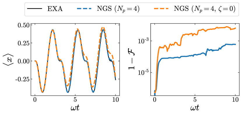
Figure 2: Comparison between multi-polaron ansatz of Eq. (1) with and without squeezing for evolution under the anharmonic oscillator, both with $N_{p}=4$ polarons. The inclusion of squeezing (blue dashed) results in closer agreement with exact numerics (solid black) compared to the absence of squeezing in the ansatz (orange dashed). However, both capture the dynamics with small infidelities $1-\mathcal{F}<\mathcal{O}(10^{-2})$. Here ${\cal F}(t)=|\langle\Psi(t)|\psi(t)\rangle|$, where $\ket{\Psi(t)}$ is the quantum state obtained with exact numerics.

Example: Quantum anharmonic oscillator As an example of the results of the above machinery, and to illustrate the role of squeezing in the ansatz, we use Eq. (4) and solve for the dynamics of a simple anharmonic oscillator, $H=\omega a^{\dagger}a+\mu(a^{\dagger}a)^{2}$  Milburn (1986); Halpern (1973); Bender and Wu (1973, 1969). Results for the strong coupling regime setting $\omega=\mu=1$ are shown in Fig. 2 with $N_{p}=4$. We observe that the ansatz containing squeezing (dashed blue line) has a better agreement with the actual state $\ket{\Psi}$ (solid black line, obtained using exact solution of the Schrödinger equation) than the ansatz without squeezing (dashed orange line). While this observation always depends on the specific system being studied, we observe that for many applications in this work the improvement in accuracy from including squeezing comes at the expense of additional computational resources. Motivated by this, for the remainder of this article we consider a multi-polaron ansatz containing only the (many-mode) coherent states.

III Open Dynamics: Combining NGS with quantum trajectories

To extend the NGS machinery to open dynamics there are several options available. For instance, in Ref. Schlegel et al. (2023), which in turn builds on the developments in Ref. Joubert-Doriol and Izmaylov (2015), an NGS analog for the density matrix was developed. This was then used to formulate the master equation and find the corresponding equations of motion governed by the Lindbladian.

Here, we discuss how the ansatz introduced previously, $\ket{\psi(\vec{z},t)}$ in Eq. (1), can be used within the quantum trajectories framework. In Sec. III.1 we recall the basic formulation of the quantum trajectories approach before formulating equations of motion for the effective non-Hermitian Hamiltonian in Sec. III.2. We give a recipe for how to formulate the action of quantum jumps within the NGS ansatz in Sec. III.3, and we finally discuss the relevant issues related to the implementation of the equations of motion in Sec. III.4. To elucidate the formalism, we provide specific examples throughout this section. Our examples are motivated by typical sources of decoherence in spin-boson quantum simulation platforms governed by Hamiltonians of the form introduced in Sec. V.

III.1 Quantum trajectories

Many problems of dynamics of open quantum systems are amenable to the standard time-local master equation in the Lindblad form Breuer and Petruccione (2002); Weiss (2012); Gardiner and Zoller (2004)

$$\dot{\rho}=-i[H,\rho]+\sum_{m}c_{m}\rho c_{m}^{\dagger}-\frac{1}{2}\left\{c_{m}^{\dagger}c_{m},\rho\right\},$$ (19)

where $c_{m}$ are the jump operators and $\{\cdot,\cdot\}$ the anticommutator.

An alternative approach is to use the quantum trajectories method Dalibard et al. (1992); Mølmer et al. (1993); Plenio and Knight (1998); Daley (2014). Here, rather than evolving the full density matrix described by $2^{2N_{s}}$ elements (for $N_{s}$ spin-1/2 particles), one stochastically evolves a pure quantum state $\ket{\psi}$ described by $2^{N_{s}}$ elements. This approach consists of two steps: (i) continuous evolution under the Schrödinger equation with an effective non-Hermitian Hamiltonian, $H_{\text{eff}}=H-\frac{i}{2}\sum_{m}c^{\dagger}_{m}c_{m}$ and (ii) discrete evolution under the action of a quantum jump operator $c_{m}$. Such stochastic evolution of the wavefunction $\ket{\psi}$ constitutes a quantum trajectory. Observables of interest are then evaluated by averaging over $n_{\rm traj}$ such quantum trajectories. In scenarios where it is possible to obtain the observables of interest with sufficient accuracy using $n_{\rm traj}<2^{N_{s}}$, quantum trajectories can be more efficient as compared to solving the master equation Mølmer et al. (1993); Daley (2014); Preisser et al. (2023).

Our key contribution is to perform (i) using NGS. The details of the quantum trajectories method, and a step by step description of its implementation, can be found in Ref. Daley (2014).

III.2 Equations of motion for non-Hermitian Hamiltonians

In between the quantum jumps, the wavefunction evolves continuously under the effective non-Hermitian Hamiltonian,

$$H_{\rm eff}=H-\frac{i}{2}\sum_{m}c_{m}^{\dagger}c_{m}=H-iK.$$ (20)

Here, we follow the procedure in Ref. Yuan et al. (2019) to derive equations of motion for evolution under $H_{\rm eff}$. The NGS wavefunction evolves according to the Schrödinger equation,

$$\partial_{t}\ket{\psi}=-iH_{\rm eff}\ket{\psi}.$$ (21)

McLachlan’s variational principle requires the variation of the norm resulting from the Schrödinger equation to vanish,

$$\delta||(d/dt+iH_{\rm eff})\ket{\psi}||=0.$$ (22)

Since it is more convenient to work with the square norm, we rewrite Eq. (22) as $\delta||(d/dt+iH_{\rm eff})\ket{\psi}||^{2}=0$, obtaining

$$\begin{split}&||(d/dt+iH_{\rm eff})\ket{\psi}||^{2}=\sum_{\mu,\nu}\bra{v_{\mu}}\ket{v_{\nu}}\dot{z}_{\mu}\dot{z}_{\nu}\\ &+\left(i\bra{v_{\mu}}H_{\rm eff}\ket{\psi}\dot{z}_{\mu}+\text{h.c.}\right)+\bra{\psi}{H_{\rm eff}}^{\dagger}{H_{\rm eff}}\ket{\psi}.\end{split}$$ (23)

After making the following substitutions

$$A_{\mu\nu} =\bra{v_{\mu}}\ket{v_{\nu}},$$ (24a)

$$C_{\mu} =\bra{\psi}H\ket{v_{\mu}},$$ (24b)

$$D_{\mu} =\bra{\psi}K\ket{v_{\mu}},$$ (24c)

the variation of the square of the norm is

$$\begin{split}&\delta||(d/dt+iH_{\rm eff})\ket{\psi}||^{2}=\sum_{\mu}\sum_{\nu}\left(A_{\mu\nu}+\text{h.c.}\right)\dot{z}_{\nu}\delta z_{\mu}\\ &+\left[i(C_{\mu}^{\dagger}-iD_{\mu}^{\dagger})+\text{h.c.}\right]\delta z_{\mu},\end{split}$$ (25)

which yields equations of motion,

$$\sum_{\nu}\real[A_{\mu\nu}]\dot{z}_{\nu} =\real[D_{\mu}]+\imaginary[C_{\mu}].$$ (26)

The object $2\real[A_{\mu\nu}]$ is precisely the metric $g$ of the tangent space [introduced in Eq. (6b)], which we showed how to compute in Sec. II.2. $\real[D_{\mu}]$ can be related to $\partial_{\mu}\langle K\rangle$ via

$$2\real[\bra{v_{\mu}}K\ket{\psi}]=\bra{v_{\mu}}K\ket{\psi}+\text{h.c.}=\partial_{\mu}\langle K\rangle,$$ (27)

where we substituted the definition of the tangent vector into the definition of $D$ in Eq. (24c), and used the fact that $K=K^{\dagger}$. We showed how to analytically compute the gradient of expectation value such as $\partial_{\mu}\langle K\rangle$ in Sec. II.1. Although $\imaginary[C_{\mu}]$ can be computed by directly calculating the overlaps in the definition in Eq. (24b), if the tangent space is a Kähler manifold (i.e. $J^{2}=-1$), then from the relation $J\indices{{}^{\mu}_{\nu}}\ket{v_{\mu}}=i\ket{v_{\nu}}$ we can relate $\imaginary[C_{\mu}]$ to the complex structure $J\indices{{}^{\mu}_{\nu}}$ and the gradient $\partial_{\mu}\langle H\rangle$ using

$$\begin{split}2\imaginary[C_{\nu}]&=i\bra{v_{\nu}}H\ket{\psi}-i\bra{\psi}H\ket{v_{\nu}}\\ &=-\bra{v_{\mu}}(J\indices{{}^{\mu}_{\nu}})^{T}H\ket{\psi}-\bra{\psi}HJ\indices{{}^{\mu}_{\nu}}\ket{v_{\mu}}\\ &=-\sum_{\mu}J\indices{{}^{\mu}_{\nu}}\partial_{\mu}E.\end{split}$$ (28)

As such, the non-Hermitian equations of motion in Eq. (26) can be computed from $g$, $\partial_{\mu}\langle H\rangle$, and $\partial_{\mu}\langle K\rangle$. The total number of elements to compute scales as $M^{2}+2M$, compared to $M^{2}+M$ for purely real- or imaginary-time evolution, where $M$ is the number of variational parameters.

Example: Computing $\boldsymbol{\imaginary[C_{\mu}]}$ for the coherent state ansatz. Here, we relate ${\rm Im}[C_{\mu}]$ to energy gradients $\partial_{\mu}\langle H\rangle$ for the coherent state ansatz with explicit normalization and phase factors, $\ket{\psi}=e^{\kappa+i\theta}e^{-(x^{2}+y^{2})/2}e^{(x+iy)a^{\dagger}}\ket{0}$, with $\vec{z}=(\kappa,\theta,x,y)\in\mathbb{R}$. The tangent vectors corresponding to $\mu\in\{1,2,3,4\}$ are

$$\ket{v_{1}} =\ket{\psi},$$ (29a)

$$\ket{v_{2}} =i\ket{\psi},$$ (29b)

$$\ket{v_{3}} =(a^{\dagger}-x)\ket{\psi},$$ (29c)

$$\ket{v_{4}} =(ia^{\dagger}-y)\ket{\psi}.$$ (29d)

We begin by relating $\imaginary[C_{1}]=\imaginary[\bra{\psi}H\ket{v_{1}}]$ to $\partial_{z_{2}}E$,

$$\begin{split}\imaginary[C_{1}]&=-\frac{1}{2}[i\bra{\psi}H\ket{v_{1}}-i\bra{v_{1}}H\ket{\psi}]\\ &=-\frac{1}{2}(\bra{\psi}H\ket{v_{2}}+\bra{v_{2}}H\ket{\psi})=-\frac{1}{2}\partial_{z_{2}}E.\end{split}$$ (30)

Similarly for $\imaginary[C_{2}]=\imaginary[\bra{\psi}H\ket{v_{2}}]$, we have

$$\imaginary[C_{2}]=\frac{1}{2}\partial_{z_{1}}E.$$ (31)

To relate $\imaginary[C_{3}]=\imaginary[\bra{\psi}H\ket{v_{3}}]$ to the gradients of $E$, we notice that we can write $i\ket{v_{3}}$ as a real span of the tangent vectors $\{v_{\mu}\}$. That is, $i\ket{v_{3}}=\ket{v_{4}}+y\ket{v_{1}}-x\ket{v_{2}}$. Using this we obtain

$$\imaginary[C_{3}]=-\frac{1}{2}\left(\partial_{z_{4}}E+y\partial_{z_{1}}E-x\partial_{z_{2}}E\right),$$ (32)

and finally for $\imaginary[\bra{v_{4}}H\ket{\psi}]$, using $i\ket{v_{4}}=-\ket{v_{3}}-x\ket{v_{1}}-y\ket{v_{2}}$, we obtain

$$\imaginary[\bra{v_{4}}H\ket{\psi}]=\frac{1}{2}\left(\partial_{z_{3}}E+x\partial_{z_{1}}E+y\partial_{z_{2}}E\right).$$ (33)

Therefore, we have related the computation of $\imaginary[C_{\mu}]$ to the energy gradients of $E=\langle H\rangle$. In this example, we explicitly noticed that $i\ket{v_{\mu}}$ can be written as a real span of tangent vectors $\{v_{\mu}\}$. In the supplementary material Sec. SI, we provide the constructions of $g_{\mu\nu}$, $\omega_{\mu\nu}$ and $J\indices{{}^{\mu}_{\nu}}$ for this single mode coherent state ansatz, showing that $\ket{v_{\nu}}=J\indices{{}^{\mu}_{\nu}}\ket{\mu}$, as derived in Eq. (28). We also provide $J\indices{{}^{\mu}_{\nu}}$ of the squeezed coherent state and the multipolaron ansatz.

Finally, we provide a simple example of non-Hermitian dynamics using NGS and the equations of motion in Eq. (26) by computing the evolution of the coherent state ansatz for $N_{b}=2$ modes under $H_{\rm eff}=\sum_{j=1}^{2}\xi_{j}(a_{j}+a^{\dagger}_{j})-i/2\sum_{j=1}^{2}\kappa_{j}a^{\dagger}_{j}a_{j}$. Since the Hamiltonian is a Gaussian operator, if the initial state of interest can be accurately described by the NGS ansatz with $N_{p}$ polarons, NGS is exact in that it captures precisely the dynamics at all times also with $N_{p}$ polarons. The results for an $N_{p}=2$ initial state and a comparison against exact numerics are shown in Fig. 3, depicting perfect agreement as expected.

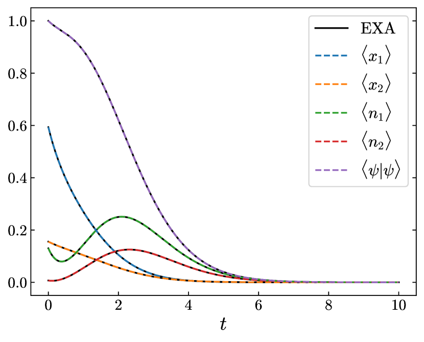
Figure 3: Dynamics of the two mode effective Hamiltonian $H_{\rm eff}=\sum_{j=1}^{2}\xi_{j}(a_{j}+a^{\dagger}_{j})-i/2\sum_{j=1}^{2}\kappa_{j}a^{\dagger}_{j}a_{j}$ with $\vec{\xi}=[0.5,0.3]$, $\vec{\kappa}=[1.0,0.6]$. The non-Hermitian term corresponds to a cavity loss jump operatos. The initial state is a random two polaron state. The NGS results (dashed colours) agree perfectly with exact numerics (solid black), including the decay of the norm $\innerproduct{\psi}{\psi}$ due to the non-hermitian term.

III.3 Quantum jumps

We will now incorporate the action of a quantum jump $c_{m}$ in the NGS formalism. After each quantum jump the wavefunction may (i) stay in the variational manifold, or (ii) leave it. We discuss these two possibilities using the examples of single particle loss and gain, respectively. We have chosen these two processes as they are often the dominant sources of single particle decoherence in a variety of systems.

(i) Jumps inside the manifold

To demonstrate the machinery of a jump operator that produces a state contained within the variational manifold, we consider single particle loss at rate $\kappa^{(1)}$. The jump operator is $c=\sqrt{\kappa^{(1)}}a$. The action of $c$ on the single-mode multi-polaron ansatz in Eq. (1) without squeezing, i.e. $|\vec{\zeta}|=0\;\forall p$, is given by,

$$\begin{split}\sqrt{\kappa^{(1)}}a\ket{\psi}&=\sqrt{\kappa^{(1)}}a\sum_{p}e^{\kappa_{p}+i\theta_{p}}D(\alpha_{p})\ket{0}\\ &=\sum_{p}\sqrt{\kappa^{(1)}}e^{\kappa_{p}+i\theta_{p}}\alpha_{p}D(\alpha_{p})\ket{0}\\ &=\sum_{p}e^{\kappa_{p}^{\prime}+i\theta_{p}^{\prime}}D(\alpha_{p})\ket{0},\end{split}$$ (34)

where we used $a\ket{\alpha}=\alpha\ket{\alpha}$ and defined the updated norm and phase factors as

$$\kappa_{p}^{\prime} =\log(\sqrt{\kappa^{(1)}}e^{\kappa_{p}}\absolutevalue{\alpha_{p}}),$$ (35a)

$$\theta_{p}^{\prime} =\arg(\absolutevalue{\kappa^{(1)}}e^{i\theta_{p}+\kappa_{p}}\alpha_{p}).$$ (35b)

We can easily extend the above analysis to the two-photon loss case with the jump operator $c=\sqrt{\kappa^{(2)}}a^{2}$, where the updated norm and phase factors are now defined as

$$\kappa_{p}^{\prime} =\log(\sqrt{\kappa^{(2)}}e^{\kappa_{p}}\absolutevalue{\alpha_{p}}^{2}),$$ (36a)

$$\theta_{p}^{\prime} =\arg(\sqrt{\kappa^{(2)}}e^{i\theta_{p}+\kappa_{p}}\alpha_{p}^{2}).$$ (36b)

It is important to note that our results rely on the coherent state being the eigenstate of the jump operator considered above. Thus, for any other state, e.g. the squeezed coherent state $\ket{\alpha,\zeta}$, the single-particle loss jump operator will take the state out of the variational manifold. This will be a more generic scenario for most jump operators. In the next section we describe how to deal with such situations.

(ii) Jumps outside the manifold

If the state after the jump is not within the variational manifold, we project it back to the manifold by maximizing its fidelity with the variational states. To do so we use gradient descent (GD) as an efficient numerical procedure. We note that while simulated annealing (SA) finds a global extremum of a function in the asymptotic limit of infinitely slow cooling rate, we find that in all cases studied in this work, the performance of GD is comparable to that of SA (the infidelity difference between the post-jump variational state found by each of the two methods is $\lesssim 10^{-3}$), with the advantage that it is typically significantly faster.

Again, we consider a single mode multi-polaron ansatz with coherent states only, which we write as

$$\ket{\psi}=\sum_{i=1}^{N_{p}}c_{i}\ket{\alpha_{i}},$$ (37)

with complex coefficients $c_{i}$ and complex amplitudes $\alpha_{i}$. For single photon gain with jump operator $c=a^{\dagger}$, the state after applying the jump operator $a^{\dagger}\ket{\psi}$ is projected back back onto a generic variational state $|\tilde{\psi}\rangle$ by optimising its variational parameters $\tilde{c}_{i},\tilde{\alpha}_{i}$ to maximize the normalised fidelity given by,

$$\mathcal{F}=\frac{|\langle\tilde{\psi}|a^{\dagger}|\psi\rangle|^{2}}{{|\langle\tilde{\psi}|\tilde{\psi}\rangle|}{|\langle\psi|aa^{\dagger}|\psi\rangle|}},$$ (38)

where the un-normalised overlap is

$$\langle\tilde{\psi}|a^{\dagger}|\psi\rangle=\sum_{i,j}^{N_{p}}\tilde{c}_{i}^{*}c_{j}\tilde{\alpha}_{i}^{*}e^{-\frac{1}{2}(|\alpha|^{2}+|\tilde{\alpha}|^{2})+\tilde{\alpha}_{i}^{*}\alpha_{j}},$$ (39)

and the normalisation factors are

$$\bra{\psi}\ket{\psi} =\sum_{i,j}^{N_{p}}c_{i}^{*}c_{j}e^{-\frac{1}{2}(|\alpha_{i}|^{2}+|\alpha_{j}|^{2}+\alpha_{i}^{*}\alpha_{j})},$$ (40a)

$$\bra{\psi}aa^{\dagger}\ket{\psi} =\sum_{i,j}^{N_{p}}c_{i}^{*}c_{j}(1+\alpha_{i}^{*}\alpha_{j})$$

$$\times e^{-\frac{1}{2}(|\alpha_{i}|^{2}+|\alpha_{j}|^{2})+\alpha_{i}^{*}\alpha_{j}}.$$ (40b)

In the case of $N_{p}=1$, with $\alpha=|\alpha|{\rm e}^{i\varphi_{\alpha}}$, $\tilde{\alpha}=|\tilde{\alpha}|{\rm e}^{i\varphi_{\tilde{\alpha}}}$, Eq.  (39) is maximized for $\varphi_{\tilde{\alpha}}=\varphi_{\alpha}$ and for amplitude of $\tilde{\alpha}$ which is the solution to $|\tilde{\alpha}|^{2}-|\alpha|\,|\tilde{\alpha}|-1=0$. For instance if $\alpha=0$, $|\tilde{\alpha}|=1,\;\forall\varphi_{\tilde{\alpha}}$, cf. Fig. 4(a), and similarly for $\alpha\neq 0$, cf. Fig. 4(b). The starting point of the gradient descent search is denoted by the red cross and the maximum of the numerically found maximum of the overlap, Eq. (39), by the white cross. We remark that the achievable fidelity after projecting back to the manifold is strongly dependent on the jump operator and the number of polarons. For instance, for the case shown in Fig. 4(a), the state after the jump is a Fock state $\ket{1}$. As such, after projecting it back to a single coherent state, its fidelity is given by ${\rm e}^{-|\tilde{\alpha}|^{2}/2}|\alpha|^{n}/\sqrt{n!}\rightarrow{\rm e}^{-1/2}\approx 0.61$ with $n=1$ and $|\tilde{\alpha}|=1$.

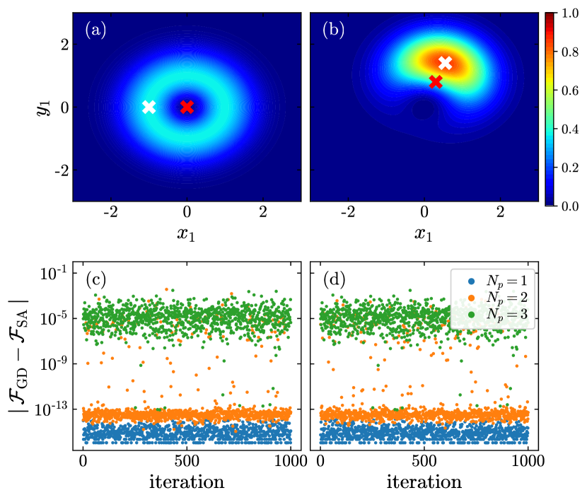
Figure 4: (a,b) Fidelity of $a^{\dagger}\ket{\alpha}$ projected back onto the variational manifold here formed by the set of all coherent states $|\tilde{\alpha}=\tilde{x}+i\tilde{y}\rangle$. The red cross denotes the initial state upon which acts the jump operator $a^{\dagger}$, and the white cross denotes the maximum of Eq. (39) found via gradient descent. The used initial states are (a) $\ket{\alpha=0}$ (with a ring of global maxima due to the symmetry of $a\ket{0}$) and (b) $\ket{\alpha=0.3+i0.8}$. (c,d) Difference in optimized fidelities, cf. Eq. (38), found by gradient descent vs. bounded simulated annealing. The jump operators are (c) $a^{\dagger}$ and (d) $x=a+a^{\dagger}$.

In the generic case of the multipolaron ansatz $N_{p}>1$, the optimization landscape becomes more complex. In Fig. 4(c)-(d), for $N_{p}=1$ (blue), $N_{p}=2$ (orange) and $N_{p}=3$ (green) we use Eq. (38) and plot the difference in optimized fidelities $|{\cal F}_{\rm GD}-{\cal F}_{\rm SA}|$, with the optimization performed by gradient descent with backtracking (${\cal F}_{\rm GD}$) and bounded simulated annealing (${\cal F}_{\rm SA}$). We consider two quantum jumps, (c) single-particle gain $c=a^{\dagger}$ and (d) momentum kicks $c=x=a+a^{\dagger}$. Our choice of single-particle gain is motivated by its relevance to many spin-boson systems (see Secs. V and VI), whilst the momentum kick jump plays a crucial role in laser cooling large ion crystals Gerritsen et al. . We generate $10^{3}$ initial (pre-jump) random states $\ket{\psi}$. As the generic variational starting state $|\tilde{\psi}\rangle$ to be optimized, for GD we use the pre-jump state $\ket{\psi}$, whilst for the SA we seed a random starting state $|\tilde{\psi}\rangle$ whose coefficients (see Eq. (37)) are drawn from a uniform unit distribution $\{c_{i},\alpha_{i},\tilde{c}_{i},\tilde{\alpha}_{i}\}\in[0,1]$. We set a sufficiently slow SA cooling rate such that the algorithm converges to the same local maxima irrespective of the randomly chosen starting point. For all the studied cases, the fidelities of the states obtained by the two numerical optimizers agree within $\lesssim 10^{-3}$.

III.4 Time evolution

We are now equipped to implement the quantum trajectories program for the NGS ansatz outlined in Sec. III.1. In principle, one could evolve the wavefunction $\ket{\psi}$ between the jumps according to the equations of motion in Eq. (26) while tracking the decay of the norm to identify the time $t_{j}$ of a jump. In practice we find it convenient to Trotterize the time evolution between jumps governed by $H_{\rm eff}$, Eq. (20), in the usual way as

$$e^{-i(H-iK)\delta t}\approx e^{-iH\delta t/2}e^{-K\delta t/2}$$ (41)

for sufficiently small $\delta t$. The norm during the unitary dynamics under ${\rm e}^{-iH\delta t/2}$ is preserved due to the use of the norm factors $\kappa$ as variational parameters (we note that the opposite case, namely the absence of a global norm factor as a variational parameter, can result in unphysical couplings, see Ref. Hackl et al. (2020)). During the imaginary-time evolution ${\rm e}^{-K\delta t/2}$ we track the decay of the norm caused to determine the time of the jump $t_{j}$, where we apply the corresponding jump operator $c_{m}$.

IV Truncated Wigner Approximation for spins and bosons

The phase space picture of quantum mechanics provides alternative means to simulate and analyze the quantum many-body dynamics in systems with mixed spin and bosonic degrees of freedom, in particular in a semi-classical framework known as the truncated Wigner approximation (TWA) Polkovnikov (2010a). The Wigner-Weyl transform maps Hilbert space operators $O$ of a quantum system to functions of classical phase space variables, known as Weyl symbols $O_{W}$. The Weyl symbol corresponding to the density matrix is known as the Wigner function and provides a full ensemble description of arbitrary quantum states in terms of a (potentially negative) quasi-probability distribution.

A general Wigner-Weyl transform can be defined using the framework of phase point operators Wootters (1987). For example, considering particles in 1D with positions $\mathbf{x}$ and momenta $\mathbf{p}$, operators $\mathcal{A}(\mathbf{x},\mathbf{p})$ for each point in phase space define the Wigner-Weyl transformation via $O_{W}(\mathbf{x},\mathbf{p})={\rm tr}[\mathcal{A}(\mathbf{x},\mathbf{p})O]/\sqrt{2\pi}$ and vice versa $O=\int d\mathbf{x}d\mathbf{p}\,O_{W}(\mathbf{x},\mathbf{p})\mathcal{A}(\mathbf{x},\mathbf{p})$. Given a proper orthonormal definition of phase point operators Wootters (1987), for any state $\rho$ and any observable $Q$, expectation values can be evaluated from the Wigner function $W(\mathbf{x},\mathbf{p})={\rm tr}[\mathcal{A}(\mathbf{x},\mathbf{p})\rho]/\sqrt{2\pi}$ via $\langle Q\rangle=\int d\mathbf{x}d\mathbf{p}\,Q_{W}(\mathbf{x},\mathbf{p})W(\mathbf{x},\mathbf{p})$. Equivalent constructions can be made for spin phase spaces, either using spin-boson mappings (suitable for large spin scenarios) Polkovnikov (2010a), using spherical coordinate representations of spins $A(\theta,\phi)$ Mink et al. (2022), or for phase spaces using only a discrete set of points Wootters (1987).

Closed-system time-evolution equations of motion can be obtained by Wigner-Weyl transforming the Heisenberg equations of motion, which leads to the exact quantum dynamics for Weyl symbols being governed by $\dot{Q}_{W}(\mathbf{x},\mathbf{p})=\{Q_{W}(\mathbf{x},\mathbf{p}),H_{W}(\mathbf{x},\mathbf{p})\}_{\rm MB}$, using the Weyl symbol of the Hamiltonian $H_{W}$, and the Moyal bracket defined as $\{Q_{W},H_{W}\}=2Q_{W}\sin(\mathbf{\Lambda/2})H_{W}$, with $\mathbf{\Lambda}$ the symplectic operator (with $\hbar\equiv 1$) $\mathbf{\Lambda}=\sum_{i}\frac{\overleftarrow{\partial}}{\partial x_{i}}\frac{\overrightarrow{\partial}}{\partial p_{i}}-\frac{\overleftarrow{\partial}}{\partial p_{i}}\frac{\overrightarrow{\partial}}{\partial x_{i}}$. Expanding the sine function in the Moyal bracket at the lowest order is know as TWA and leads to a classical evolution of Weyl symbols $\dot{Q}_{W}(\mathbf{x},\mathbf{p})\approx\{Q_{W}(\mathbf{x},\mathbf{p}),H_{W}(\mathbf{x},\mathbf{p})\}_{\rm P}$, where $\{\cdot,\cdot\}_{\rm P}$ now denotes the classical Poisson bracket. The Poisson bracket ensures that the Weyl symbols for any complex observable will always factorize into phase space variables, and therefore in TWA it suffices to only compute the classical evolution of the phase space variables Zhu et al. (2019). This makes TWA a very practical and efficient numerical method for the case of a positive initial Wigner function: Random positions and momenta can be sampled from the Wigner function and evolved in parallel using classical equations of motion giving $\mathbf{x}_{\eta}(t)$ and $\mathbf{p}_{\eta}(t)$ for trajectory $\eta$. Expectation values in TWA are then statistically approximated by $\langle Q\rangle\approx\frac{1}{n_{\rm traj}}\sum_{\eta}^{n_{\rm traj}}Q_{W}(\mathbf{x}_{\eta}(t),\mathbf{p}_{\eta}(t))$, using $n_{\rm traj}$ trajectories.

Importantly, for small-spin systems, and in particular for spin-1/2 models as considered here, TWA can be drastically improved when using a sampling of the initial Wigner function using only a discrete set of initial phase points Schachenmayer et al. (2015a). Considering a system consisting of a single spin-1/2 described by the Pauli operators $\bm{\sigma}=\left(\sigma_{x},\sigma_{y},\sigma_{z}\right)$, we define the corresponding phase space variables as ${\mathcal{S}}=\left(S_{x},S_{y},S_{z}\right)$. One can then define discrete Wigner functions which are only defined for for the 8 different discrete points $\mathbf{\mathcal{S}}_{0}=(\pm 1,\pm 1,\pm 1)$. For example, taking a state of $N_{s}$ spin-1/2 particles of the form $\ket{\psi}=\bigotimes_{i=1}^{N_{s}}\ket{\downarrow}_{i}$, it is straightforward to show that any possible observable can be exactly described by sampling each spin from a discrete Wigner function with the only non-zero values of $W^{\downarrow}_{i}(S_{x}=\pm 1,S_{y}=\pm 1,S_{z}=-1)=1/4$. Correspondingly, the state $\ket{\uparrow}_{i}$ is exactly described by the discrete distribution with non-zero elements $W_{i}^{\uparrow}(S_{x}=\pm 1,S_{y}=\pm 1,S_{z}=+1)=1/4$.

Furthermore, it can be shown in general that equivalent discrete sampling strategies can lead to exact quantum state descriptions for general discrete $D$-level systems and for eigenstates of general spin-$S$ operators, in the sense that the measurement statistics for any observable can be exactly reproduced from sampling the Wigner function Zhu et al. (2019). Discrete sampling in combination with classical evolution is known as (generalized) discrete truncated Wigner approximation, (G)DTWA Schachenmayer et al. (2015a); Zhu et al. (2019). Classical equations of motion for the spin-variables can be derived by Wigner-Weyl transforming the Heisenberg equations of motion while factorizing the Weyl symbols into the phase space variables. (G)DTWA has been shown to capture quantum features in spin-model dynamics in several theory settings Schachenmayer et al. (2015b); Acevedo et al. (2017); Kunimi et al. (2021); Perlin et al. (2020); Muleady et al. (2023), and in comparison with experiments Lepoutre et al. (2019); Orioli et al. (2018); Franke et al. (2023); Alaoui et al. (2024).

Below we will consider a system consisting not only of spins but also of bosonic $a\left(a^{\dagger}\right)$ degrees of freedom. For the bosonic part we will consider the complex numbers $a\rightarrow A$ and $a^{\dagger}\rightarrow A^{*}$ as the classical phase space. We note that for additional bosonic degrees of freedom with operators denoted as $b\left(b^{\dagger}\right)$ one can introduce a corresponding classical phase space with $b\left(b^{\dagger}\right)\to B\left(B^{*}\right)$ (see for example Sec. V). Then, considering a system with $N_{s}$ spin-1/2 particles coupled to $N_{a/b}$ bosonic modes $a/b$, computing expectation values of an observable $Q(\bm{\sigma}_{i},a_{j},b_{k})$ with TWA at time $t$ corresponds to numerically evaluating

$$\langle O \left(t;\{\bm{\sigma}_{i},a_{j},b_{k}\}\right)\rangle\approx\int\prod_{i=1}^{N_{s}}\prod_{j=1}^{N_{a}}\prod_{k=1}^{N_{b}}d\mathbf{\mathcal{S}}_{0}^{i}d^{2}A_{0}^{j}d^{2}B_{0}^{k}$$ (42)

$$W_{i}(\mathbf{\mathcal{S}}_{0}^{i})W_{j}(A_{0}^{i})W_{k}(B_{0}^{k})O_{W}\left(\{\mathbf{\mathcal{S}}_{\rm cl}^{i}(t),{A}_{\rm cl}^{j}(t),{B}^{k}_{\rm cl}(t)\}\right),$$

where $d\mathbf{\mathcal{S}}_{0}=dS_{0}^{x}dS_{0}^{y}dS_{0}^{z}$, $d^{2}A_{0}=d{\rm{Re}}A_{0}d{\rm{Im}}A_{0}/\pi$, and the subscript $0$ indicates the initial values at $t=0$. The classical variables for spin $i$ and bosons $j$ and $k$ are sampled from the initial Wigner functions $W_{i}(\mathbf{\mathcal{S}}_{0}^{i})$, $W_{j}(A_{0}^{j})$, and $W_{k}(B_{0}^{k})$, respectively. Note that we always assume an initial product state between all degrees of freedoms such that the Wigner functions factorize. For the spins we will use the discrete distributions $W^{\uparrow/\downarrow}_{i}$ defined above, while for the bosonic modes we use standard continuous Wigner functions, in particular

$$W_{j}(A_{0}^{j})=\frac{1}{2\pi w_{j}^{2}}\exp{-\absolutevalue{A_{j}-\bar{\alpha}_{j}}^{2}/(2w_{j}^{2})},$$ (43)

where $w_{j}^{2}=(\bar{n}_{j}+1/2)/2$ and $\alpha$ center of the Wigner function. For the vacuum state $\bar{n}_{j}=\bar{\alpha}_{j}=0$, while for a coherent state $\ket{\alpha}$, $\bar{n}_{j}=0$ and $\bar{\alpha}_{j}=\alpha$ (see Refs. Polkovnikov (2010b); Piñeiro Orioli et al. (2017) for more details). $O_{W}\left(\{\mathbf{\mathcal{S}}_{\rm cl}^{i}(t),{A}_{\rm cl}^{j}(t),{B}^{k}_{\rm cl}(t)\}\right)$ is the Weyl symbol corresponding to the observable of interest. We use the subscript cl on the time-dependent variables $\mathbf{S}^{i}_{\rm cl}(t)$, $A^{j}_{\rm cl}(t)$, and $B^{k}_{\rm cl}(t)$ to indicate that they obey the classical equations of motion for spin $i$, boson $j$, and boson $k$, respectively. In Sec. V below we will provide the full classical equations of motion for our problem of interest for examples of both closed and open system dynamics. (G)DTWA methods have been recently developed further to also include open-system dynamics under Lindblad master equations Huber et al. (2021, 2022); Singh and Weimer (2022); Mink et al. (2022); Mink and Fleischhauer (2023). For our simulations we follow the procedure in Ref. Mink et al. (2022) and use a spherical coordinate parametrization of the phase space for spin $i$ with phase point operators defined as

$$\mathcal{A}_{i}(\theta_{i},\phi_{i})=\frac{1}{2}[\mathbb{1}_{i}+\mathbf{s}(\theta_{i},\phi_{i})\cdot\bm{\sigma}_{i}],$$ (44)

where we use the vector on the surface of a sphere with radius $\sqrt{3}$, $\mathbf{s}_{i}=\sqrt{3}\left(\sin{\theta_{i}}\cos{\phi_{i}},-\sin{\theta_{i}}\sin{\phi_{i}},-\cos{\theta_{i}}\right)^{\intercal}$.

In Mink et al. (2022) it was shown that for open spin-1/2 models, it is convenient to work with flattened Wigner functions of the form $\chi_{i}(\theta_{i},\phi_{i})\equiv W_{i}(\theta_{i},\phi_{i})\frac{\sin\theta_{i}}{2\pi}$. The equations of motion for an open system can then be found by deriving correspondence rules (reminiscent of Bopp representations for for bosonic systems Polkovnikov (2010a)), i.e. rules for mapping terms such as $X_{i}\rho_{i}$, $\rho_{i}X_{i}$, or $X_{i}\rho_{i}X_{i}^{\dagger}$ with Pauli operators $X=\sigma_{i}^{x,y,z}$ to the phase space, which leads to terms incorporating the 4 linearly independent differential operations $\mathbb{1},\frac{d}{d\theta_{i}},\frac{d}{d\phi_{i}},\frac{d^{2}}{d\phi_{i}^{2}}$ acting on $\chi(\theta_{i},\phi_{i})$. It can be shown that the resulting EOMs lead to standard Fokker-Planck equations. This is only valid, without further approximations, for systems of non-interacting spins or if the initial state is a large coherent spin state. In these scenarios, the dynamics are given by the solution to the Fokker-Planck equations.

In our discrete sampling we select the initial angles $\theta_{i},\phi_{i}$ according to the parametrization given in Eq. (43). However, rather than sampling from the discrete $W_{i}^{\uparrow/\downarrow}$ Wigner distribution, we sample from a slightly modified flattened Wigner function

$$\chi^{\uparrow/\downarrow}(\theta,\phi)=\frac{1}{2\pi}\delta(\theta\pm\arccos{\frac{1}{\sqrt{3}}}),$$ (45)

which is generated by rotating the discrete Wigner function $W_{i}^{\uparrow/\downarrow}$ around the z-axis. This initial Wigner function is uniform in $\phi$ and thus guarantees that $\frac{\partial^{2}}{\partial\phi_{m}\partial(\theta_{n}-\theta_{n+1})}$ cross diffusion terms, which are dropped in TWA, vanish at $t=0$ Mink et al. (2022). For more details, we refer the reader to Ref. Mink et al. (2022) and Sec. V where the detailed equations for our problem of interest are introduced.

V Results

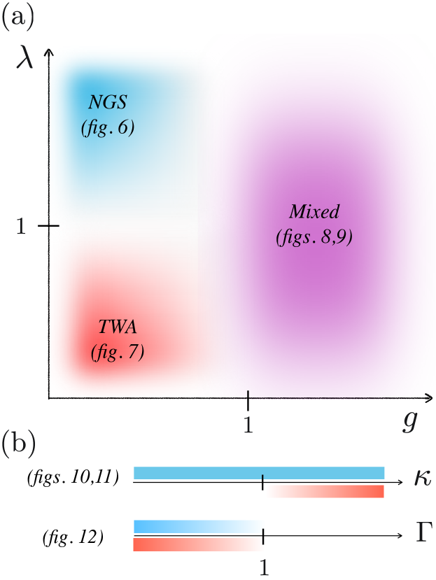
Figure 5: Schematic of the performance of TWA and NGS for (a) closed and (b) open dynamics. In the present study NGS is limited to at most $N_{p}=16$ polarons and no squeezing. (a) The performance in $g-\lambda$ parameter space for closed dynamics. When $g,\lambda\lesssim 1$, TWA performs well, whilst when $g\lesssim 1,\lambda\gtrsim 1$, NGS is the better choice. When $g\gtrsim 1$, TWA captures short-time dynamics, but can produce incorrect mid- to late-time results. In comparison, NGS typically does not capture quantitative details beyond the first spin relaxation, but does provide qualitative insights into the dynamics by correctly capturing the magnitude of the persistent spin-cavity dynamics. (b) Open dynamics. We operate in the $g\lesssim 1$, $\lambda\gtrsim 1$ region, so NGS outperforms TWA at small $\kappa$. At large $\kappa$, TWA performs well again, with both NGS and TWA agreeing. When evolving under only $H_{\rm TC}$ with the spins decaying collectively at rate $\Gamma$, NGS and TWA agree when using the large $N_{s}$ Holstein-Primakoff (HP) transformation at small $\Gamma$. At large $\Gamma$ the collective spin quickly decays to the ground state, which is inaccessible as the first order expansion of the root in HP is no longer sufficient near the ground state since it was expanded around the excited state (small $a^{\dagger}a$), so neither method is able to capture intermediate- to late-time dynamics.

To evaluate the performance of our two numerical methods, we consider the disordered Holstein-Tavis-Cummings model describing a system of $N_{s}$ spins $\sigma$ coupled to a single bosonic mode ($a$), representing a coupling to a cavity mode, and $N_{s}$ local vibrational modes ($b_{i}$) associated with each spin. The system is described by the Hamiltonian Wellnitz et al. (2022):

$$H=H_{\rm TC}+H_{\rm vib}+H_{\rm H}+H_{\rm dis},$$ (46)

where

$$H_{\rm TC} =\frac{\Delta}{2}\sum_{j=1}^{N_{s}}(\sigma^{z}_{j}+\mathbb{1})+\frac{g}{\sqrt{N_{s}}}\sum_{j=1}^{N_{s}}a\sigma_{j}^{+}+a^{\dagger}\sigma_{j}^{-},$$ (47a)

$$H_{\rm vib} =\nu\sum_{j=1}^{N_{s}}b^{\dagger}_{j}b_{j},$$ (47b)

$$H_{\rm H} =-\frac{\lambda\nu}{2}\sum_{j=1}^{N_{s}}(b_{j}+b_{j}^{\dagger})(\sigma_{j}^{z}+\mathbb{1}),$$ (47c)

$$H_{\rm dis} =-\frac{1}{2}\sum_{j=1}^{N_{s}}\epsilon_{j}(\sigma^{z}_{j}+\mathbb{1}),$$ (47d)

where $\Delta$ describes the detuning of the spin transition frequency relative to the cavity mode, $g/\sqrt{N_{s}}$ the single-spin coupling to the cavity, $\nu$ the frequency of the vibrational modes, $\lambda$ the relative strength of the Holstein coupling, and $\epsilon_{j}$ the disorder in the transition frequency for spin $j$.

The dynamics of the Holstein-Tavis-Cummings model, in particular in the presence of disorder, has importance e.g. in the field of polaritonic chemistry Herrera and Spano (2016). It has been previously studied using a matrix product state method Wellnitz et al. (2022), and also using a similar non-Gaussian state framework to the one discussed here Sun et al. (2022). By tuning the relative strength of the various terms, this Hamiltonian can be reduced to spin-boson Hamiltonians applicable e.g. to trapped ion quantum simulators, impurity models, and quantum chemistry. The relative strength of $g,\lambda,$ and $\nu$ allows us to go from the weak coupling regime between the spin and bosonic degrees of freedom, to a model governed by a Tavis-Cummings type interaction, a Holstein coupling, or a combination thereof. We illustrate the performance of our methods in these regimes schematically in Fig. 5(a).

Furthermore, we investigate how both methods perform in the presence of sources of decoherence. In this case, we are interested in the evolution of the density matrix $\rho$ as described by the Lindblad master equation,

$$\dot{\rho}=-i[H,\rho]+\sum_{m}c_{m}\rho c_{m}^{\dagger}-\frac{1}{2}\left\{c_{m}^{\dagger}c_{m},\rho\right\},$$

where $c_{m}$ are the jump operators and $\{\cdot,\cdot\}$ is the anticommutator. We study open dynamics with the following types of Lindblad jump operators:

• Cavity decay (rate $\kappa)$: $c_{m}=\sqrt{\kappa}a$,

• Single spin decay (rate $\gamma$): $c_{m}=\sqrt{\gamma}\sigma^{-}_{i}$, and

• Collective spin decay (rate $\Gamma$) $c_{m}=\sqrt{\Gamma}\sum_{i}\sigma^{-}_{i}$.

We summarize the performance of the two methods in the presence of these decoherence sources schematically in Fig. 5(b).

V.1 Details of NGS and TWA simulations

We consider two scenarios for evolution under the Hamiltonian (46). In the first case ($\epsilon,\,\lambda=0$), the evolution reduces to evolution under $H_{\rm TC}$ and therefore takes places in the collective Tavis-Cummings manifold as $H_{\rm TC}$ conserves the total excitation number $N_{\rm ex}=a^{\dagger}a+\sum_{i}\sigma_{i}^{z}$. Away from this limit, when $\epsilon\neq 0$ or $\lambda\neq 0$, the spins can no longer be treated as a large collective spin and thus must be treated as an interacting collection of single spin-$1/2$ systems.

V.1.1 Tavis-Cummings

When the evolution is under $H_{\rm TC}$ we can use the Holstein-Primakoff (HP) transformation to map the collective spin $S$ to a single bosonic mode,

$$S_{+} =\sqrt{2s-a^{\dagger}a}\,a,$$ (48a)

$$S_{z} =s-a^{\dagger}a,$$ (48b)

where $s\equiv N_{s}/2$. We use a Taylor series to expand the square root in powers of $1/s$ to first order. The NGS simulation then proceeds using the multipolaron ansatz with $N_{b}=2$ bosonic modes. We can include collective spin decay $\sum_{i}\sigma_{i}^{-}$ at strength $\Gamma$ using the manifold projection technique described in Sec. (III.3).

For the TWA simulations, the equations of motion for the cavity mode $A$ and the large spin HP mode $B$ are,

$$\dot{A}_{\rm cl} =-\frac{\kappa}{2}A_{\rm cl}-i\frac{g}{2\sqrt{2s}}B_{\rm cl}^{*}\left(4s-N_{B,\rm cl}\right),$$ (49a)

$$\dot{N}_{A,\rm cl} =-\kappa N_{A,\rm cl}-\frac{g}{\sqrt{2s}}\imaginary[A_{\rm cl}B_{\rm cl}]\left(4s-N_{B,\rm cl}\right),$$ (49b)

$$\begin{split}\dot{B}_{\rm cl}&=\Gamma B_{\rm cl}\left[s-\frac{1}{8s}+N_{B,\rm cl}\left(\frac{\absolutevalue{B_{\rm cl}}^{2}}{16s}-\frac{1}{2}\right)\right]\\ &\hphantom{={}}+\frac{ig}{2\sqrt{2s}}\left[A_{\rm cl}B_{\rm cl}^{2}-2A_{\rm cl}^{*}\left(2s-N_{B,\rm cl}\right)\right]+i\Delta B_{\rm cl},\end{split}$$ (49c)

$$\dot{N}_{\rm cl} =\Gamma\left[2S+N_{B,\rm cl}\left(\frac{1}{4s}+2\left(s-1\right)+\mathcal{F}(B_{\rm cl})\right)\right]$$

$$-\frac{g}{\sqrt{2s}}\imaginary[A_{\rm cl}B_{\rm cl}](4s-N_{B,\rm cl}),$$ (49d)

where we introduce the function $\mathcal{F}(B_{\rm cl})=\frac{1}{8s}\absolutevalue{B_{\rm cl}}^{2}\left(4-8s+\absolutevalue{B_{\rm cl}^{2}}\right)$. We sample the cavity (mode A) assuming a coherent state $\ket{\alpha=1}$ and sample the large spin (mode B) assuming the spins are polarised pointing up, which corresponds to sampling the vacuum for mode B.

Our results using this approach, including collective spin decay, are shown in Fig. 12 in the lines labeled as TWA (HP) and NGS (HP).

V.1.2 Holstein Tavis-Cummings

In principle the NGS ansatz can be used directly to treat the spin degrees of freedom. However, to avoid the explicit exponential scaling with $N_{s}$, we again use a Holstein-Primakoff transformation to map each spin-$1/2$ to a bosonic mode. We use a different form of the HP transformation Vogl et al. (2020),

$$S_{+} =(1-a^{\dagger}a)a,$$ (50a)

$$S_{z} =1/2-a^{\dagger}a,$$ (50b)

as unlike the usual HP transformation used above in Eq. (48), it is exact for spin-$1/2$. As such, the dynamics are restricted to the $\ket{0}\equiv\ket{e}$ and $\ket{1}\equiv\ket{g}$ subspace, with $\outerproduct{g}{g}=a^{\dagger}a$ and $\outerproduct{e}{e}=1-a^{\dagger}a$. The vacuum is a Gaussian state and can therefore be described using only $N_{p}=1$. The Fock state $\ket{1}$ can be described using $N_{p}=2$, by $\ket{1}=1/\mathcal{N}\lim_{\alpha\rightarrow 0}(\ket{\alpha}-\ket{-\alpha})$, where $\mathcal{N}$ is a normalization factor Marshall and Anand (2023), with $\alpha\sim 0.001$ sufficient to describe the state with high fidelity. As such, each spin can be captured using $N_{p}=3$ polarons.

For the NGS simulations, we employ the NGS ansatz with $N_{b}=2N_{s}+1$ modes. We include cavity decay at strength $\gamma$ using the simple parameter-update prescription outlined in Sec. V Note that as a consequence of this mapping, the ansatz is not well-suited to some scenarios. For example, there is no spin-spin coupling when evolving under only $H_{\rm dis}$, so an unentangled initial state will evolve as a tensor product of single spins, each requiring $N_{p}=3$. The number of polarons therefore scales exponentially in the number of spins, $3^{N_{s}}$. This limitation could potentially be circumvented by modifying the ansatz to be a superposition of squeezing displaced Fock states Schlegel et al. (2023).

For the TWA simulations, to more accurately capture the dynamics of the cavity and vibrational modes, we extend the set of TWA equations by including the classical equations of motion for the mode excitation numbers $a^{\dagger}a\rightarrow N_{A},b_{k}^{\dagger}b_{k}\rightarrow N_{B_{k}}$. Including all three sources of decoherence described above, the equations of motion for the spin degrees of freedom are,

$$\begin{split}\dot{\theta}_{i,\rm cl}&=(\Gamma+\gamma)(\cot\theta_{i,\rm cl}-\frac{\csc\theta_{i,\rm cl}}{\sqrt{3}})\\ &+\frac{2g}{\sqrt{N_{s}}}\imaginary[e^{-i\phi_{i,\rm cl}}A_{\rm cl}]\\ &-\frac{\Gamma\sqrt{3}}{2}\sum_{j}\cos{(\phi_{i,\rm cl}-\phi_{j,\rm cl})}\sin{\theta_{j,\rm cl}},\end{split}$$ (51a)

$$\begin{split}d\phi_{i,\rm cl}&=\big{(}-\Delta+\epsilon_{n}+2\lambda\nu\real[B_{i,\rm cl}]\\ &-\frac{2g}{\sqrt{N_{s}}}\cot{\theta_{i,\rm cl}}\real[A_{\rm cl}e^{-i\phi_{i,\rm cl}}]\\ &-\frac{\Gamma\sqrt{3}}{2}\sum_{j}\cot{\theta_{i,\rm cl}}\sin{\theta_{j,\rm cl}}\sin{(\phi_{i,\rm cl}-\phi_{j,\rm cl})}\big{)}dt\\ &+\sqrt{(\Gamma+\gamma)f(\theta_{i,\rm cl})}dW_{\phi_{i}},\end{split}$$ (51b)

where we introduced the function $f(\theta_{i,\rm cl})=1+2\cot{\theta_{i,\rm cl}}^{2}-2\cot{\theta_{i,\rm cl}}\csc{\theta_{i,\rm cl}}/\sqrt{3}$. The equations of motion for the bosonic degrees of freedom are given by

$$\dot{A_{\rm cl}} =-\frac{\kappa}{2}A_{\rm cl}-i\frac{\sqrt{3}g}{2\sqrt{N_{s}}}\sum_{i}e^{i\phi_{i,\rm cl}}\sin{\theta_{i,\rm cl}},$$ (52a)

$$\dot{N}_{A,\rm cl} =-\kappa N_{A,\rm cl}-\frac{\sqrt{3}g}{\sqrt{N_{s}}}\sum_{i}\sin{\theta_{i,\rm cl}}\imaginary[A_{\rm cl}e^{-i\phi_{i,\rm cl}}],$$ (52b)

$$\dot{B}_{k,\rm cl} =-i\nu B_{k,\rm cl}+i\frac{\lambda\nu}{2}\left(1-\sqrt{3}\cos{\theta_{k,\rm cl}}\right),$$ (52c)

$$\dot{N}_{B_{k,\rm cl}} =\lambda\nu\left(1-\sqrt{3}\cos{\theta_{k,\rm cl}}\right)\imaginary[B_{k,\rm cl}].$$ (52d)

Finally, we note that the initial state used for all NGS simulations includes a small amount of randomness for each variational parameter to break the degeneracy of the Gaussian states. We draw random values from a flat distribution between $(0,10^{-4})$. We find that this is sufficient to ensre each Gaussian state in the superposition evolves independently, whilst ensuring extremely small infidelity with the true initial state, $1-\mathcal{F}(t=0)<\mathcal{O}(10^{-6})$, as seen in Fig. S1 of the supplementary material.

V.2 Closed system dynamics

In this section we compare the performance of the two numerical methods. We consider a system with $N_{s}=3$ spins, the corresponding three phonon modes, and one cavity mode. For this system size and suitable initial states and Hamiltonian parameters, choosing a moderate Fock state truncation $\sim 10$ allows us to compare our results to exact numerics. Our initial state is spins polarized up, the vibrational modes in the vacuum, and the cavity in a coherent state, $|\psi(0)\rangle=|{\uparrow}\rangle^{\otimes N_{s}}|\alpha=1\rangle_{a}|0\rangle_{b}^{\otimes N_{s}}$. Note in contrast to Ref. Sun et al. (2022) our initial state is a superposition of several excitation manifolds precluding further simplifications to the ansatz.

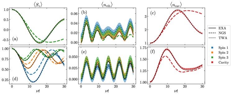
Figure 6: Closed dynamics: $g=\lambda=0.1$, $\Delta=0$. Top row: without disorder. Both NGS and TWA capture the initial spin relaxation, but NGS incorrectly predicts a slower revival. Bottom row: disordered, $\vec{\epsilon}=[2g,3g,4g]$. Here, TWA captures the dynamics more accurately compared to NGS. NGS is with $N_{p}=4$, TWA is with $n_{\rm traj}=10^{4}$ with standard error shaded.

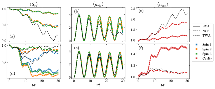
Figure 7: Closed dynamics: $g=0.1,\lambda=1$, $\Delta=0$. Top row: without disorder. Neither TWA nor NGS completely capture the spin-cavity observables, but NGS more closely tracks the dynamics Bottom row: disordered, $\vec{\epsilon}=[2g,3g,4g]$. NGS performs well, capturing all dynamics with small error. Interestingly, here TWA over estimates the magnitude of changes in the spin-cavity observables. Here NGS uses $N_{p}=12$, TWA is with $n_{\rm traj}=10^{4}$ with standard error shaded.

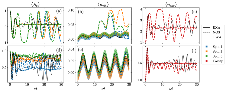
Figure 8: Closed dynamics: $g=1$, $\lambda=0.1$, $\Delta=0$. Top row: without disorder. Beyond initial spin relaxation, both TWA and NGS perform relatively poorly. TWA incorrectly predicts equilibration of the spin-cavity dynamics. NGS does continue to produce spin-cavity dynamics, but overestimates the magnitude of the oscillations. Bottom row: disordered, $\vec{\epsilon}=[2.6g,3.2g,4.2g]$. TWA incorrectly predicts equilibration of both spin and cavity observables after the first oscillation, whilst NGS produces qualitatively correct dynamics, even with only $N_{p}=4$ polarons. Here NGS uses $N_{p}=2$ for the first row and $N_{p}=4$ for the second row, and TWA is with $n_{\rm traj}=10^{4}$ with standard error shaded.

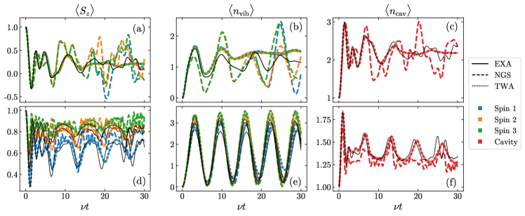
Figure 9: Closed dynamics: $g=1$, $\lambda=1$, $\Delta=0$. Top row: without disorder. TWA accurately captures the dynamics at early times as compared to the NGS. Bottom row: disordered, $\vec{\epsilon}=[2.6g,3.2g,4.2g]$. TWA correctly captures key oscillations, even at late times. NGS also captures some of these features, but less accurately. Both methods perform similarly for the vibrational dynamics. Here NGS uses $N_{p}=4$, TWA is with $n_{\rm traj}=10^{4}$ with standard error shaded.

For all closed dynamics simulations, we set $\Delta=0$. For evolution under the Holstein-Tavis-Cummings model in Eq. (46), we find that while both methods are good at capturing the short time dynamics, at later times they out-perform one another in different parameter regimes. We summarise our findings in Fig. 5(a), where we qualitatively depict the performance for different parameter regimes in the absence of decoherence. More detailed dynamics for each regime are plotted in Figs. 6-9, with the first and second rows of each figure showing dynamics without and with disorder $\epsilon$, respectively.

We begin in the weak coupling regime $g=\lambda=0.1$, shown in Fig. 6. Here the dynamics is slow on the considered time-scale. In both the disorder-free (first row) and disordered (second row) settings, NGS and TWA accurately capture the small fluctuations of the vibrational modes at all times. Both methods also capture the initial spin relaxation, however NGS misses the revival time. TWA’s ability to capture the first oscillation appears universally in all of the parameter regimes considered in this work. This behaviour can be understood as follows: due to our choice of a factorisable initial state with a corresponding positive semi-definite Wigner function, the TWA sampling is able to reproduce the initial state, and the mean-field and low order correlations that are generated during the short-time dynamics.

A generic feature of TWA is that when extending into the medium- to long-time dynamics, the potential buildup of higher order correlations is not captured by the method. While this not visible in Fig. 6, it can be seen clearly in the figures corresponding to the regimes discussed below.

The second regime we consider is the strong spin-vibrational coupling $\lambda\gg g$, shown in Fig. 7. Here we expect NGS to perform well, as NGS is exact with any polaron number for $H_{\rm H}$. In the disorder-free regime (top row), although NGS with $N_{p}=12$ does not fully capture the dynamics at late times, it does outperform TWA, which majorly underestimates the spin decay. In this case, the lack of disorder is challenging for our multi-polaron NGS ansatz: each spin evolves identically, requiring the multi-polarons to be factored into a product. This symmetry is broken when introducing disorder (second row), and we see that NGS captures accurately the dynamics for all considered times, including the initial decay and then revival of $\langle S_{z}\rangle$. For TWA, although the numerics match better for the vibrational dynamics in the presence of disorder, this is primarily a consequence of the fact that the disorder causes the Holstein interactions to dominate, and the spin and cavity dynamics continue to disagree with the exact solution.

Thirdly, we move to the strong spin-cavity coupling regime, $g\gg\lambda$, shown in Fig. 8. After accurately capturing the first oscillation, the TWA spin dynamics equilibrate about $\langle S_{z}\rangle\sim 0$ unlike the exact dynamics which, although they do oscillate about $\langle S_{z}\rangle\sim 0$, exhibit persistent oscillations with magnitude $\langle S_{z}\rangle\sim 1/2$. Similarly, NGS with $N_{p}=4$ polarons fails to capture any of the spin, vibration, or cavity dynamics. This is unsurprising because, in this regime where the Tavis-Cummings term dominates, we expect the number of polarons required to scale as $\sim 3^{N_{s}}$, as each spin must be described using $N_{p}=3$ polarons. Although increasing $N_{p}$ would eventually improve the accuracy, we found that increasing it up to $N_{p}\lesssim 16$ did not provide a substantial increase in accuracy, whilst increasing the computational cost. In principle, TWA does not suffer from the same problem. However, if one needs to access higher order correlations with TWA, the introduction of higher order cumulants and the BBGKY hierarchy may become necessary. This poses an analogous problem to the polaron number: an exponentially increasing number of equations and potential numerical instabilities .

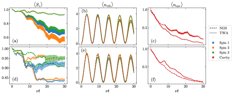
Figure 10: Open dynamics. $g=0.1$, $\lambda=1$, $\Delta=0$ and cavity decay $\kappa=g$. Top row: without disorder. Bottom row: with disorder $\vec{\epsilon}=[2g,3g,4g]$. NGS and TWA capture the same short-time dynamics, but disagree beyond $\nu t\sim 5$. Based on the corresponding closed dynamics results Fig. 7, we expect NGS to be more reliable in this regime. Exact numerics is challenging for open dynamics of systems of this size, see Fig. S2 for benchmarking of smaller systems. Here NGS uses $N_{p}=8$ and $n_{\rm traj}=40$ with standard error indicated by the error bars, TWA is with $n_{\rm traj}=10^{4}$ with standard error shaded.

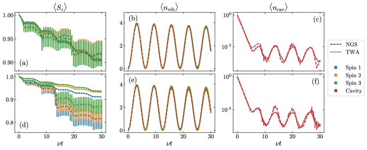
Figure 11: Open dynamics. $g=0.1$, $\lambda=1$, $\Delta=0$ and cavity decay $\kappa=10g$. Top row: without disorder. Bottom row: with disorder $\vec{\epsilon}=[2g,3g,4g]$. We observe compatible results for the spins and a remarkable agreement between NGS and TWA for the vibrational and cavity dynamics, including the small amplitude oscillations in $\langle n_{\rm cav}\rangle$ at late times. Here NGS uses $N_{p}=8$ and $n_{\rm traj}=40$ with standard error indicated by the error bars, TWA is with $n_{\rm traj}=10^{4}$ with standard error shaded.

Fourthly, we consider the strong spin-cavity and spin-vibration regime $\lambda=g=1$, shown in Fig. 9. Without disorder, both methods struggle to capture the dynamics at late times, although TWA in particular is able to capture qualitative features with reasonable accuracy. Introducing disorder breaks the collective nature of the spins, enabling both methods to more accurately track the dynamics. TWA is able to qualitatively reproduce the periodic peaks in the spin and cavity dynamics at even later times than NGS. Both methods correctly obtain the vibrational dynamics.

Finally, we note that an advantage of NGS is the accessibility of the wavefunction. This means that any desired quantity, including entanglement entropy, can be computed. Furthermore, for small systems, strict performance measures such as the fidelity can be easily computed. These are shown in Fig. S1 for the four different coupling regimes $(g,\lambda)$ considered in Figs. 6-9. The analogous plots for TWA cannot be generated.

V.3 Open system dynamics

Next, we introduce decoherence to our simulations. Figs. 10 and 11 show the spin and bosonic dynamics for $N_{s}=3$ in the presence of cavity loss $a$ at strength $\kappa=g$ (Fig. 10) and $\kappa=10g$ (Fig. 11), and in the regime $\lambda\gg g$, where NGS provides more accurate predictions in the closed setting (cf. Fig. 7). In the top row we set the disorder $\epsilon=0$, while the bottom row shows the dynamics in the presence of disorder, $\vec{\epsilon}=[2g,3g,4g]$. Although exact dynamics were accessible for a closed system of this size, obtaining exact results in this open dynamics setting is challenging. In Fig. S2 we compare the two methods with exact results for a smaller system.

For these parameters, we find that, perhaps unsurprisingly, NGS continues to perform well in both $\kappa=g$ and $\kappa=10g$ decoherence regimes. In the weaker decay limit shown in Fig. 10, NGS and TWA agree only at short times. The under- and over-estimation of spin-cavity dynamics by TWA in the non-disordered and disordered systems respectively is consistent with the behaviour of TWA in the closed system, see Fig. 7. In the large decay limit shown in Fig. 11, NGS and TWA are in reasonable agreement with one another for the spin dynamics and in near total agreement for the vibrational and cavity dynamics. Both show fast decay of the cavity to the vacuum, and remarkably both capture small oscillatory dynamics at late times with excellent agreement. Physically, both methods demonstrate that strong cavity decay stabilises the spin dynamics, which we attribute to the reduction of the effective Tavis-Cummings coupling strength and the prevention of the build up of correlations in the system between the spins, as well as spin-boson correlations, due to the loss of cavity excitations.

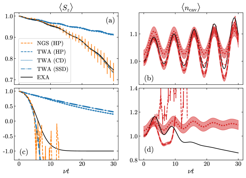
Figure 12: Collective spin dynamics. $\nu=\epsilon=\lambda=0$, $\Delta=1$, $g=0.1$. Top row: $\Gamma=0.1g/\sqrt{N_{s}}$. NGS (HP) and TWA (HP) use the Holstein-Primakoff representation of the collective spin and agree excellently with exact numerics (EXA). On the other hand, when TWA treats the spins individually, the collective decay dynamics TWA (CD) agrees with the single spin decay dynamics TWA (SSD), but both deviate from the exact evolution due to TWA’s failure to capture the correlations. Bottom row: $\Gamma=g/\sqrt{N_{s}}$. NGS (HP) and TWA (HP) agree with exact numerics (EXA) until $t\nu\sim 5$, when the first order Taylor series expansion of the HP mapping breaks down. Here NGS uses $N_{p}=8$ and $n_{\rm traj}=40$ with standard error indicated by the error bars, TWA is with $n_{\rm traj}=10^{4}$ with standard error shaded.

Next, we consider the effect of spin decay. We consider the scenario where the Hamiltonian evolution is only under $H_{\rm TC}$ and the spins decay collectively at a rate $\Gamma$. We set $\Delta=1$ and $g=0.1$. Within the TWA formalism we treat the dynamics using two methods. First, we continue to treat the system as a collection of individual spins, as described in Sec. IV. In Fig. 12 we plot the resulting dynamics where TWA (CD) refers to implementing this sampling in the presence of collective spin decay at $\Gamma=0.1g/\sqrt{N_{s}}$ and $g/\sqrt{N_{s}}$. TWA (SSD) uses the same sampling but the decay mechanism is single spin at the corresponding rate. The agreement between the two, and the disagreement with exact numerics (EXA) indicates that treating the spins individually with either of these two methods is inadequate to simulate collective spin decay.

This motivates our second strategy, described in Sec. V.1.1, where we use the HP formalism for large spins, which we apply to both NGS and TWA. In the weak spin decay limit $\Gamma=0.1g/\sqrt{N_{s}}$, both NGS (HP) and TWA (HP) are in excellent agreement with the exact numerics (EXA). NGS in particular captures the cavity dynamics with little error, whilst the error bars on the spin dynamics are still somewhat large due to our use of relatively few trajectories, $n_{\rm traj}=40$. In the large decay limit $\Gamma=g/\sqrt{N_{s}}$, both NGS and TWA correctly capture the rapid spin decay until $\nu t\sim 5$. Beyond this point, the first order Taylor series expansion of the HP mapping breaks down, as highly excited Fock states are populated. One can potentially circumvent this issue by simulating collective spin decay as was done in Ref. Young et al. (2024) with DTWA. There, the spins were collectively coupled to a single cavity whose cavity loss was much stronger than the collective spin-cavity coupling, resulting in effective collective spin decay and without the utilization of the HP mapping. Comparing the performance of these approaches in different parameter regimes and for different models, e.g., for more complex forms of collective spin decay, represents an interesting future direction.

VI Conclusions and outlook

Summary and conclusions: In this work, we presented a non-Gaussian variational ansatz approach to studying the dynamics of open quantum systems composed of spin and bosonic degrees of freedom. While several other works in recent years have utilized NGS to study the time evolution of open quantum systems, previous efforts have focused on developing an equivalent ansatz for the density matrix and simulating the Lindblad equations. Here, we utilized the quantum trajectories method, allowing us to take advantage of the previously developed machinery and analytic expressions obtained for real- and imaginary-time dynamics.

In addition to providing a comprehensive overview of this method, we performed extensive numerical simulations over a broad range of parameters of a spin-boson Hamiltonian [Eq. (46)] with Tavis-Cummings (TC) and Holstein couplings, which is applicable to a broad range of quantum simulation platforms as well as problems of interest in quantum chemistry, atomic physics and condensed matter theory. We compared the performance of NGS with a method using the truncated Wigner approximation for systems with mixed bosonic and spin degrees of freedom, extended to open quantum systems following the approach in Ref. Mink et al. (2022).

In the absence of decoherence our findings are as follows: for strong TC coupling, TWA is the more accurate method, while for strong Holstein couplings NGS is the better choice. When neither term dominates, for both weak and strong coupling regimes, TWA captures the short-time dynamics, while NGS generally displays the correct qualitative behaviour, even at late times. After introducing spin disorder the performance of NGS typically improves, whilst for TWA the vibrational dynamics match the exact dynamics better, which is attributable to the fact that disorder causes the Holstein interaction to dominate.

For open quantum dynamics we focused on the regime where the Holstein term dominates and considered the effect of cavity loss. At weak decay rates the NGS continues to perform well. TWA improves as the cavity decay rate increases due to the loss of quantum correlations, with both NGS and TWA showing excellent agreement. In the presence of collective spin decay we considered the TC model only, finding that in the limit of small collective decay, both methods perform well when using a Holstein-Primakoff transformation for the large spin. In the limit of large collective decay, NGS and TWA both only capture the short time dynamics as the Holstein-Primakoff transformation is no longer accurate at later times. Using TWA we were able to also treat each spin individually. However, TWA does not capture the collective nature of the decay, with the results closely matching the effect of single spin decay.

Further considerations should also be made when deciding between the two methods. Although the NGS ansatz can be made less computationally demanding by reducing the polaron number $N_{p}$, in general TWA methods are easier to implement and require fewer computational resources. The resource requirement and the complexity of NGS is offset by the advantages that it is a controlled approximation and gives access to the wavefunction, allowing one to access any observable, including higher-order correlations. The TWA framework needs to be amended if one hopes to capture these correlations accurately. A potential strategy to remedy this can be to use a cluster TWA approach Wurtz et al. (2018). There, several sub-system parts are grouped into a single (discrete or continuous) large sub-system that, provided a proper sampling strategy, follows the fully exact quantum evolution, while correlations between clusters are approximated in TWA. Such approaches allow to use the cluster size as controllable parameter to enhance the simulation towards the exact one.

Outlook: The extension of NGS to open quantum systems using the quantum trajectories formulation that we presented in this work is perhaps the most natural pathway. For Hermitian jump operators, an alternative approach and a simple extension of this work would be to instead solve the stochastic partial differential equations that result from the unravelling of the master equation. Furthermore, one could explore the impact of the chosen unraveling on the performance of the NGS method at a fixed $N_{p}$, as it has been shown that this choice can have a large effect on the entanglement buildup in the trajectory Vovk and Pichler (2022, 2024).

Another limitation of the present formulation is that the spin states in Eq. (1) are exact and span the full spin Hilbert space of dimension $2^{N_{s}}$, thus limiting the use of the ansatz to a handful of spins unless approximations such as the large $N_{s}$ expansion in the Holstein-Primakoff mapping used in Sec. V.1.1 are invoked. On the one hand, studies using a fermionic Gaussian state representation of spins have been performed Kaicher et al. (2023), and these might be combined in principle in a straightforward way with the multipolaron ansatz for bosons Shi et al. (2018). On the other hand, it would be highly interesting to combine the multipolaron ansatz with other variational techniques highly suitable for the spins such as tensor network based approaches Schollwöck (2011); Orús (2014); Montangero (2018). Furthermore, similar to the present comparison between NGS and TWA, it would be beneficial to apply the here-presented non-Gaussian ansatz to the study of other systems which might be challenging to simulate otherwise. These include for instance purely bosonic models, such as the Bose-Hubbard model, with disorder and on non-regular lattices Gottlob and Schneider (2023). Such extensive studies will allow for a comparison between our approach and the corresponding master equation approach based on extending the ansatz of Eq. (1) to density matrices Schlegel et al. (2023); Joubert-Doriol and Izmaylov (2015).

Finally, we note that a particular promising application field of the methodologies introduced here could be in the emerging field of polaritonic chemistry Hutchison et al. (2012); Simpkins et al. (2021); Wang and Yelin (2021); Campos-Gonzalez-Angulo et al. (2023). There, recent experiments have demonstrated that large collective strong cavity couplings (e.g. $g_{c}=g\sqrt{N}$) can be functionalized to modify chemical reactivity. A theoretical understanding for such modifications are currently centered around the question how delocalized polaritonic state can play a role for changing chemistry on the single-molecule level, as local amplitudes of collective polaritons vanish in the thermodynamic limit. In spin-boson approximations to the problems, in particular for the disordered Holstein-Tavis-Cummings Herrera and Spano (2016) model that we studied here, it was recently discovered that the interplay of disorder and collective cavity couplings can give rise to robust local quantum effects in the large-$N$ limit in the form of non-Gaussian distributions of the nuclear coordinate Wellnitz et al. (2022). Using matrix product state methods, it was possible to push simulations to systems with 160 effective molecules, but in particular the TWA approach discussed here would allow access to much larger systems. Typical parameter regimes discussed here are well covered by the TWA approach (e.g. the typical parameters from Wellnitz et al. (2022) corresponds to $\lambda\sim 0.1\nu$ and $g\ll\nu$) and thus hint to a general applicability of the method in the relevant regime. Further, the TWA approach can be straightforwardly adapted to simulate nuclear dynamics not only on harmonic but also arbitrary potential energy surfaces, whilst the NGS ansatz using the machinery presented here can also model anharmonic Hamiltonian terms. In the future this may allow for the analysis of quantum effects in realistic chemical reaction models, even in a macroscopic limit.

Supplemental Material

SI On the complex structure of the multipolaron ansatz

In this section we specify the geometric structures for special cases of the general NGS ansatz. We begin with the example of a coherent state ansatz with explicit normalization and phase factors, $\ket{\psi(\vec{z})}=e^{\kappa+i\theta}\mathcal{D}(x+iy)\ket{0}$, with $\vec{z}=\{\kappa,\theta,x,y\}$. The tangent vectors for this ansatz were given in Eq. (29a), from which we can compute the metric and symplectic forms,

$$\qquad g_{\mu\nu}=\left(\begin{array}[]{cccc}1&0&0&0\\ 0&1&-z_{4}&z_{3}\\ 0&-z_{4}&1+z_{4}^{2}&-z_{3}z_{4}\\ 0&z_{3}&-z_{3}z_{4}&1+z_{3}^{2}\end{array}\right),\qquad\omega_{\mu\nu}=\left(\begin{array}[]{cccc}0&1&-z_{4}&z_{3}\\ -1&0&0&0\\ z_{4}&0&0&0\\ -z_{3}&0&-1&0\end{array}\right)$$ (S9)

as well as their respective inverses

$$\qquad G=\left(\begin{array}[]{cccc}1&0&0&0\\ 0&1+z_{3}^{2}+z_{4}^{2}&z_{4}&-z_{3}\\ 0&z_{4}&1&0\\ 0&-z_{3}&0&1\end{array}\right),\qquad\Omega=\left(\begin{array}[]{cccc}0&-1&0&0\\ 1&0&-z_{3}&-z_{4}\\ 0&z_{3}&0&-1\\ 0&z_{4}&1&0\end{array}\right).$$ (S18)

Note that here the use of the pseudo-inverse would give the same as the inverse, as $\omega_{\mu\nu}$ and $g_{\mu\nu}$ are not singular for any values of the variational parameters $\vec{z}$. We can also compute the complex structure, $J\indices{{}^{\mu}_{\nu}}=-G^{\mu\sigma}\omega_{\sigma\nu}$,

$$J\indices{{}^{\mu}_{\nu}}=\left(\begin{array}[]{cccc}0&-1&z_{4}&-z_{3}\\ 1&0&-z_{3}&z_{4}\\ 0&0&0&-1\\ 0&0&1&0\end{array}\right),$$ (S23)

and verify that $J^{2}=-\mathbb{1}$. Using the relation $i\ket{v_{\nu}}=J\indices{{}^{\mu}_{\nu}}\ket{v_{\mu}}$ which holds if the tangent space of the variational manifold is a Kähler manifold as is the case here, we directly obtain the relations

$$i\ket{v_{1}} =\ket{v_{2}},$$ (S24)

$$i\ket{v_{2}} =-i\ket{v_{1}},$$ (S25)

$$i\ket{v_{3}} =z_{4}\ket{v_{1}}-z_{3}\ket{v_{2}}+\ket{v_{4}},$$ (S26)

$$i\ket{v_{4}} =-z_{3}\ket{v_{1}}+z_{4}\ket{v_{2}}-\ket{v_{3}},$$ (S27)

which we derived explicitly and used in the main text to compute $\text{Im}[C_{\mu}]$, see Sec. III.2.

Next, we compute the complex structure of the squeezed coherent state, including norm and phase factors, $\ket{\psi(\vec{z})}={\rm e}^{\kappa+i\theta}\ket{\alpha,\zeta}={\rm e}^{\kappa+i\theta}D(\alpha)\xi(\zeta)\ket{0}$, such that $\vec{z}=(\kappa,\theta,x,y,r,\phi)$ with $\alpha=x+iy$, $\zeta=r{\rm e}^{i\phi}$. Using the expressions in Eqs. (17), (18) we arrive at

$$J=\left(\begin{array}[]{cccccc}0&1&-y&x&0&\sinh^{2}(r)/2\\ -1&0&t_{1}&t_{2}&\tanh(r)/2&0\\ 0&0&-\sinh(2r)\sin(\phi)&\sinh(2r)\cos(\phi)+\cosh(2r)&0&0\\ 0&0&\sinh(2r)\cos(\phi)-\cosh(2r)&\sinh(2r)\sin(\phi)&0&0\\ 0&0&0&0&0&\sinh(r)\cosh(r)\\ 0&0&0&0&-\text{csch}(r)\sech(r)&0\\ \end{array}\right),$$ (S34)

where we introduced $t_{1}=\cosh^{2}(r)\left[x\tanh^{2}(r)+x-2\tanh(r)(x\cos(\phi)+y\sin(\phi))\right]$ and $t_{2}=\sinh(2r)(y\cos(\phi)-x\sin(\phi))+y\cosh(2r)$. It is straightforward to verify that

$$J^{2}=-1,$$ (S35)

i.e. the tangent space of the single-polaron single-mode ansatz is a Kähler space. A technical remark is in order. We note that

$$\det(g)=\det(\omega)\propto\sinh(2r)^{2},$$ (S36)

which vanishes in the limit of vanishing squeezing $r\rightarrow 0$ and consequently $G=g^{-1}$ is ill-defined (an alternative way of seeing this is an overparametrization of the tangent vector space as $\ket{v_{6}}$ vanishes, cf. the Eqs. (S37) below). When such situation occurs, one can use instead the Moore-Penrose pseudo-inverse, as suggested in Hackl et al. (2020), to evaluate $g^{-1}$. In this case we recover $J^{2}=-1$ and thus the Kähler space. Finally, when using Eq. (S34) in Eq. (LABEL:eq:projection) we arrive at the following tangent vectors (in addition to $\{\ket{v_{\mu}}\}$)

$$i\ket{v_{1}} =\ket{v_{2}},$$ (S37a)

$$i\ket{v_{2}} =-\ket{v_{1}},$$ (S37b)

$$\begin{split}i\ket{v_{3}}&=y\ket{v_{1}}-[x\cosh(2r)-(x\cos(\phi)+y\sin(\phi))\sinh(2r)]\ket{v_{2}}\\ &+\sin(\phi)\sinh(2r)\ket{v_{3}}+[\cosh(2r)-\cos(\phi)\sinh(2r)]\ket{v_{4}},\end{split}$$ (S37c)

$$\begin{split}i\ket{v_{4}}&=-x\ket{v_{1}}-[y\cosh(2r)+[y\cos(\phi)-x\sin(\phi)]\sinh(2r)]\ket{v_{2}}\\ &-[\cosh^{2}(r)+\sinh^{2}(r)+\cos(\phi)\sinh(2r)]\ket{v_{3}}-\sin(\phi)\sinh(2r)\ket{v_{4}},\end{split}$$ (S37d)

$$i\ket{v_{5}} =-\frac{1}{2}\tanh(r)\ket{v_{2}}+\frac{\sech^{2}(r)}{\tanh(r)}\ket{v_{6}},$$ (S37e)

$$i\ket{v_{6}} =-\frac{1}{2}\sech^{2}(r)\ket{v_{1}}-\frac{\tanh(r)}{\sech(r)^{2}}\ket{v_{5}}.$$ (S37f)

It is apparent from the above equations that the set $\{i\ket{v_{\mu}}\}$ lies in the tangent space spanned by $\{\ket{v_{\mu}}\}$ as a consequence of it being the Kähler manifold, $J^{2}=-1$.

The same procedure then generalizes to the construction of tangent vectors for each polaron $p\in\{1,\ldots,N_{p}\}$ and each mode $k\in\{1,\ldots,N_{b}\}$ such that the tangent space remains Kähler manifold also in the generic many-polaron multi-mode case. In this case the complex structure $J$ takes a block-diagonal form, where each block is labeled by the polaron and mode number $(p,k)$ with the property $J^{2}=-1$, which we could also verify numerically.

SII Benchmarking dynamics with single spin

A key advantage of NGS is that it provides access to the wavefunction $\ket{\psi}$, meaning that any desired quantity can be computed, including for example the entanglement entropy. We provide a simple example of this utility by computing the infidelity $1-\mathcal{F}(t)=1-|\innerproduct{\psi(t)}{\Psi(t)}|^{2}$ between NGS wavefunction $\ket{\psi}$ with $N_{p}=8$ and the exact wavefunction $\ket{\Psi}$ for closed real-time dynamics. This is shown in Fig. S1 for $N_{s}=1$ for the four parameter regimes studied in Figs. 6-9 (there with $N_{s}=3$). Note that such a comparison for more spins becomes challenging as we cannot access exact numerics. We find that in all regimes except $g=\lambda=1$, the infidelity of NGS is low, with $1-\mathcal{F}<\mathcal{O}(10^{-2})$. We also note that the infidelity is not accessible in TWA.

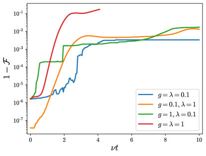
Figure S1: Infidelity $1-\mathcal{F}(t)=1-|\innerproduct{\psi(t)}{\Psi(t)}|^{2}$ of real-time dynamics for $N_{s}=1$ between NGS $\ket{\psi}$ using $N_{p}=8$ and exact $\ket{\Psi}$ for the same four parameter regimes studied in the main text. The initial infidelity is due to introducing a tiny randomness in the NGS initial state of the bosonic modes, which is a strategy we adopt to lift the degeneracy between the different polarons to avoid overparametrization of the equations of motion, cf. Bond et al. (2024). In all regions except $g=\lambda=1$ where the rapid decrease in infidelity leads to unstable NGS EOMs, NGS captures the dynamics even at late times with excellent infidelity, $1-\mathcal{F}<\mathcal{O}(10^{-2})$.

Next, we benchmark both TWA and NGS against exact numerics for open real-time dynamics. In Fig. S2, we consider $N_{s}=1$ in the same parameter regime as the main text $g=0.1,\lambda=1$ with cavity loss $\sqrt{\kappa}a$ at rates $\kappa=g$ (top row) and $\kappa=10g$ (bottom row). For weaker cavity loss $\kappa=g$ we find that NGS with $N_{p}=8$ polarons more closely tracks the exact numerics than TWA, particularly for the cavity dynamics which shows excellent agreement. At strong cavity decay rates $\kappa=10g$ both methods accurately capture the cavity dynamics, with NGS also capturing the spin decay, albeit with large error bars as only $n_{\rm traj}=40$ trajectories were used.

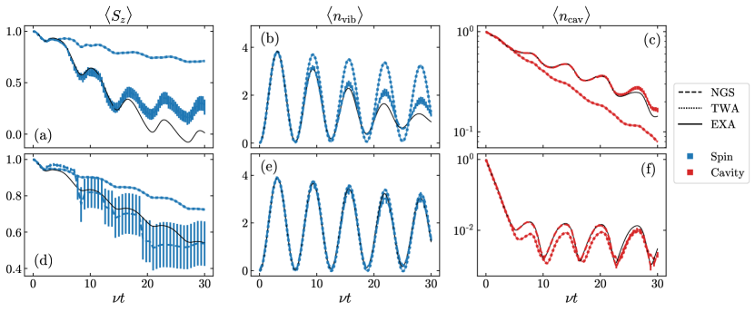
Figure S2: Benchmarking NGS and TWA against exact numerics. We use $N_{s}=1$ spin in the $g=0.1$, $\lambda=1$ regime with cavity loss $\sqrt{\kappa}a$, i.e. the same parameters considered in the main text (there with $N_{s}=3$). Top row: weaker cavity decay $\kappa=g$. NGS accurately captures the cavity dynamics, and captures the spin and vibrational mode decay until $\nu t\sim 15$. TWA significantly under-estimates the spin and vibrational decay, while over-estimating the cavity decay. Bottom row: strong cavity decay $\kappa=10g$. Both methods capture the decay of cavity population and subsequent small oscillations, as well as the vibrational loss. NGS now agrees with exact numerics for the spin decay (albeit with large error bars due to the limited $n_{\rm traj})$. TWA still underestimates this observable, although the agreement is closer. We attribute this to the loss of quantum correlations due to the decoherence which makes it easier for the TWA to capture the true quantum state. Here NGS uses $N_{p}=8$ and $n_{\rm traj}=40$ with standard error indicated by the error bars, TWA is with $n_{\rm traj}=10^{4}$ with standard error shaded.