Towards Federated Learning with on-device Training and Communication in 8-bit Floating Point

Bokun Wang bokunw.wang@gmail.com Texas A&M UniversityCollege Station, USA Axel Berg axel.berg@arm.com Arm/Lund UniversityLund, Sweden Durmus Alp Emre Acar durmusalpemre.acar@arm.com ArmBoston, USA  and  Chuteng Zhou Chu.Zhou@arm.com ArmBoston, USA
(2024)
Abstract.

Recent work has shown that 8-bit floating point (FP8) can be used for efficiently training neural networks with reduced computational overhead compared to training in FP32/FP16. In this work, we investigate the use of FP8 training in a federated learning context. This brings not only the usual benefits of FP8 which are desirable for on-device training at the edge, but also reduces client-server communication costs due to significant weight compression. We present a novel method for combining FP8 client training while maintaining a global FP32 server model and provide convergence analysis. Experiments with various machine learning models and datasets show that our method consistently yields communication reductions of at least 2.9x across a variety of tasks and models compared to an FP32 baseline.

copyright: acmlicensedjournalyear: 2024doi: XXXXXXX.XXXXXXXconference: Make sure to enter the correct conference title from your rights confirmation emai; August 25, 2024; Barcelona, Spainisbn: 978-x-xxxx-XXXX-X/YY/MM

1. Introduction

Lots of data is generated daily on personal smartphones and other devices at the edge. This data is very valuable for training machine learning models to provide services such as better voice recognition or text completion. However, the local data carries sensitive personal information which needs to be protected for privacy reasons. Furthermore, communication of local data between billions of devices and data centers is expected to occupy lots of network bandwidth and transmission is costly in terms of power consumption, which is a primary concern for edge devices running on batteries.

Despite these constraints, it is still possible to train a model without having to transmit this local data using federated learning (McMahan et al., 2017). In federated learning, each local device performs training locally with their local data and update their local models. When it comes to communication, the central server receives local models from a subset of devices. The central server then aggregates these local models and transmits a new global model back to those devices for a model update. In this way, no local data is ever exposed during communication and the global model can learn from local data as communication goes on.

Since its inception, new techniques around federated learning have been proposed to reduce communication cost. The local models, albeit smaller than the local data, are still expensive to transmit via wireless communication and will be taxing on local devices’ battery life if performed very frequently. One method to reduce communication cost is to quantize the models before the communication occurs, and several works have shown that this can be done without significant loss in model accuracy (Gupta et al., 2023; Hönig et al., 2022; Ni et al., 2024). Nevertheless, standard quantization of the model weights will introduce a bias term that slows down convergence of the training process. In order to alleviate this problem, the use of stochastic rounding has been proposed (Zheng et al., 2020; Bouzinis et al., 2023). Hence, when aggregating the client models at the server, the stochastic rounding errors tend to zero as the number of clients grows large. This method has also been shown to improve the learning process from a privacy perspective (Youn et al., 2023). Furthermore, He et al. (He et al., 2020) showed that stochastic rounding in conjunction with non-linear quantization can reduce the number of communication rounds to reach convergence even more.

Refer to caption
Figure 1. Overview of federated learning with local FP8 on-device training and weight quantization in both uplink and downlink communication.

In this paper, we focus on the use of a new type of short floating point number format which has not yet been explored for federated learning: 8-bit floating point (FP8). An 8-bit floating point number is only ¼ of the length of a 32-bit floating point number. Therefore, it has smaller representation power and lower precision than full 32-bit floating point number format, but it offers great savings in terms of model storage and memory access. Computation can be greatly accelerated with the FP8 format because of significantly less bit-wise operations required compared to FP32/FP16. Application of FP8 number format to deep learning model training and inference is in a nascent stage but is widely expected to have fast growth.

While integer representations, such as INT8, have been widely adopted for neural network quantization for efficient inference, the use of FP8 remains relatively new in comparison and has been more focused on model training. A few recent works (Wang et al., 2018; Sun et al., 2019; Peng et al., 2023) have proposed centralized neural network training in FP8 with promising results. However, for some networks, the FP8 precision was found to be insufficient for retaining accuracy in certain operations. Notably, the backwards pass through the network typically requires higher dynamic range than the forward pass. To this end, Micikevicius et al. (Micikevicius et al., 2022) proposed a binary interchange FP8 format that uses both E4M3 (4-bit exponent and 3-bit mantissa) and E5M2 (5-bit exponent and 2-bit mantissa) representations, which allows for minimal accuracy drops compared to FP16 across a wide range of network architectures. Concurrent work by Kuzmin et al. (Kuzmin et al., 2022) proposed a similar solution, where the exponent bias is flexible and updated for each tensor during training, which allows for maintaining different dynamic ranges in different parts of the network.

Being a very efficient training datatype, FP8 is a good candidate for on-device training at the edge and its industrial support points to wide-spread real-world applications. A future scenario where edge devices can perform efficient on-device training with native hardware support introduces a new class of federated learning problems. It also increases device heterogeneity in a federated learning setting, where participating devices and servers may have different levels of hardware support for FP8.

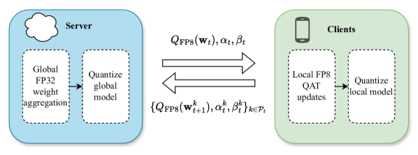
In this work, we introduce an implementation of federated learning with on-device FP8 training simulated by quantization-aware training (QAT), which learns from quantized models effectively while being efficient in its communication and computing cost. A high-level overview is shown in Figure 1. We present theoretical convergence properties as well as thorough experiments on a variety of models and data sets. Finally, we also present a novel server-side weight aggregation method that improves the server model accuracy compared to standard federated averaging.

2. Method

Preliminaries. Consider the federated learning problem, where $K$ clients update their local models by training on disjoint local datasets $\{\mathcal{D}_{k}\}_{k=1}^{K}$. Each client minimizes their own local objectives $F_{k}(\mathbf{w},Q,\alpha,\beta)=\mathbb{E}_{(\mathbf{x},y)\sim\mathcal{D}_{k}}[l(\mathbf{w};\mathbf{x},y,Q,\alpha,\beta)]$, where $Q$ is a quantization operator and $l$ is the loss function. Furthermore, $\alpha$ and $\beta$ are the per-tensor clipping values used for weights and activations respectively. Henceforth, we denote quantized weights based on range $\alpha$ as $Q(\mathbf{w};\alpha)$. In practice, different clipping values are used for different layers of the network, but we omit this in our notation for readability. The overall problem can be expressed as

(1) $\displaystyle\min_{\mathbf{w}}F(\mathbf{w},Q,\alpha,\beta),\quad F(\mathbf{w},Q,\alpha,\beta)=\sum_{k=1}^{K}\frac{n_{k}}{n}F_{k}(\mathbf{w},Q,\alpha,\beta),$

where $n_{k}=|\mathcal{D}_{k}|$ is the number of training samples on the $k$:th device and $n=\sum_{k}n_{k}$ is the total number of training examples.

On-Device Quantization-Aware Training. Depending on the hardware support, on-device local training can be performed in native FP8 or using quantization-aware training (QAT), or a mix of the two. Native FP8 training is supported by the latest AI hardware in data centers such as Nvidia’s H100/H200 series of GPUs. There is significant industry support behind FP8, it is only a matter of time for FP8 hardware support to arrive on edge devices. For research purposes, we here resort to QAT, and follow the FP8 QAT method described in (Kuzmin et al., 2022), using per-tensor quantization for both model weights and activations, with one signed bit, and $m=3$ and $e=4$ bits for the mantissa and exponent respectively, as well as a flexible exponent bias. QAT with both weights and activations quantization is a good way of simulating native FP8 training on supported hardware with low precision arithmetic. In our setting, we are not simulating the effect of gradient quantization which happens on FP8-enabled hardware. However, previous work (Kuzmin et al., 2022) has shown that it is a good approximation to ignore its effect.

Let $\mathbf{x}=(x_{1},...,x_{d})^{T}\in\mathbb{R}^{d}$ denote an FP32 input tensor and $Q_{\text{det}}:\mathbb{R}^{d}\rightarrow\mathbb{R}^{d}$ the FP8 deterministic quantization operator with a clipping parameter $\alpha$, whose element-wise outputs are given by $Q_{\text{det}}(x_{i};\alpha)=s_{i}\left\lfloor\frac{x_{i}}{s_{i}}\right\rceil$. Here, $s_{i}$ is the scale that is computed as

(2) $\displaystyle\log_{2}s_{i}=\begin{cases}\left\lfloor\log_{2}|x_{i}|+b\right\rfloor-b-m,\quad&\left\lfloor\log_{2}|x_{i}|+b\right\rfloor>1\\ 1-b-m,\quad&\text{otherwise,}\end{cases}$

where the exponent bias depends on the clipping value $\alpha$ as $b=2^{e}-\log_{2}\alpha+\log_{2}(2-2^{-m})-1$. At training time, $\alpha$ is first initialized using the maximum absolute value of each weight range, and then treated as a learnable parameter that is updated during training. Furthermore, the gradients of the non-differentiable rounding operators are computed using the straight-through estimator (Bengio et al., 2013), i.e. $\frac{\partial\left\lfloor x_{i}\right\rceil}{\partial x_{i}}=1$, with a key exception being $\left\lfloor\log_{2}|x_{i}|+b\right\rfloor$, which is treated as a constant following the approach in Kuzmin et al. (2022). Activations are quantized using the same procedure, but with a separate clipping value $\beta$.

Unbiased Quantized Communication. When applying FP8 QAT to a federated leaning scenario, an important aspect is the ability to reduce communication overhead by transferring weights between clients and the server using only 8 bits per scalar value. On client devices with hardware for FP8 mixed-precision training support, a copy of high-precision master weights (Vishwanath, 2019) is present as in our QAT setup. Therefore, at the end of each communication round, the participating clients need to perform a hard reset of their master weights to the de-quantized FP8 values on a quantization grid. This approach allows for cost reduction in both the uplink and downlink communication.

At each communication round $t$, active clients $\mathcal{P}_{t}$ will send the FP8-quantized weights to the central server together with the clipping parameters. However, to form an unbiased estimate of the average client weight, we need a different quantization operator. We therefore introduce stochastic quantization as

(3) $\displaystyle Q_{\text{rand}}(x_{i};\alpha)=s_{i}\begin{cases}\left\lceil\frac{x_{i}}{s_{i}}\right\rceil&p\leq\frac{x_{i}}{s_{i}}-\left\lfloor\frac{x_{i}}{s_{i}}\right\rfloor\\ \left\lfloor\frac{x_{i}}{s_{i}}\right\rfloor&\text{otherwise,}\end{cases}$

where $p$ is a Bernoulli random variable that takes the values 0 and 1 with equal probability. It is straightforward to verify that this randomized quantization is unbiased from a statistics point of view while the deterministic quantization introduced earlier is biased.

The quantized weights are then aggregated at the server using a federated average as $\mathbf{w}_{t+1}\leftarrow\sum_{k\in\mathcal{P}_{t}}\frac{n_{k}}{m_{t}}Q_{\text{rand}}(\mathbf{w}^{k}_{t+1};\alpha^{k}_{t+1})$, where $m_{t}=\sum_{{k^{\prime}}\in\mathcal{P}_{t}}n_{k^{\prime}}$. The clipping values are also aggregated, but without quantization, their contribution to the communication overhead is small relative to the weights. The aggregated weights are then quantized again to FP8 and transmitted to the next set of active clients with a new set of quantization parameters.

Algorithm 1 FP8FedAvg-UQ, FP8FedAvg-UQ+
$\mathbf{w}_{1},\alpha_{1},\beta_{1},Q_{\text{det}},Q_{\text{rand}}$
for $t=1,...,T$ do
     Sample a set $\mathcal{P}_{t}\in[K]$ of $P$ active devices
     for each client $k\in\mathcal{P}_{t}$ do
         Receive $Q_{\text{rand}}(\mathbf{w}_{t};\alpha_{t}),\alpha_{t},\beta_{t}$ from server
         $\{\mathbf{w}^{k}_{t+1},\alpha^{k}_{t+1},\beta^{k}_{t+1}\}\leftarrow\text{LocalUpdate}(\mathbf{w}_{t},Q_{\text{det}};\alpha_{t},\beta_{t},\mathcal{D}_{k})$
         Send $Q_{\text{rand}}(\mathbf{w}^{k}_{t+1};\alpha^{k}_{t+1}),\alpha^{k}_{t+1},\beta^{t+1}_{i}$ to server
     end for
     Compute $m_{t}=\sum_{k\in\mathcal{P}_{t}}n_{k}$, $\beta_{t+1}\leftarrow\sum_{k\in\mathcal{P}_{t}}\frac{n_{k}}{m_{t}}\beta^{k}_{t+1}$
      Compute $\mathbf{w}_{t+1}\leftarrow\sum_{k\in\mathcal{P}_{t}}\frac{n_{k}}{m_{t}}Q_{\text{rand}}(\mathbf{w}^{k}_{t+1};\alpha^{k}_{t+1})$
      $\alpha_{t+1}\leftarrow\sum_{k\in\mathcal{P}_{t}}\frac{n_{k}}{m_{t}}\alpha^{k}_{t+1}$
     $\{\mathbf{w}_{t+1},\alpha_{t+1}\}\leftarrow\textsc{ServerOptimize}(\{\alpha^{k}_{t+1},\mathbf{w}^{k}_{t+1}\}_{k\in\mathcal{P}_{t}})$
end for
Evaluate on $\mathbf{w}_{T+1},\alpha_{T+1},\beta_{T+1}$

Server-Side Optimization (ServerOptimize). The standard federated average of the weights in the un-quantized scenario corresponds to the minimization of weighted mean squared error (MSE) between the server parameters and the client parameters. However, when the server parameters are quantized before transmission to the clients, this property no longer holds. We therefore propose a modification to the server-side model aggregation, where the MSE is explicitly minimized. This can be done without communication overhead since all computations are done on the server. We are leveraging the computing power of the server to do more optimization since the server typically possesses more computing power than a device. At time step $t$, we perform model/parameters aggregation to obtain $\mathbf{w}_{t+1},\alpha_{t+1}$ for the next communication round by minimizing the following mean-squared error (MSE).

$\displaystyle\mathbf{w}_{t+1},\alpha_{t+1}=\operatorname*{arg\,min}_{\mathbf{w},\alpha}\sum_{k\in\mathcal{P}_{t}}\frac{n_{k}}{m_{t}}\|Q_{\text{rand}}(\mathbf{w};\alpha)-Q_{\text{rand}}(\mathbf{w}^{k}_{t};\alpha^{k}_{t})\|^{2}_{2}.$

Note that when there is no communication quantization, the closed-form solution to ServerOptimize is the federated average $\mathbf{w}_{t+1}=\sum_{k\in\mathcal{P}_{t}}\frac{n_{k}}{m_{t}}\mathbf{w}_{t}^{k}$. Since the problem above has no closed-form solution for the quantized communication case, we use the alternating minimization approach to optimize $\mathbf{w}$ and $\alpha$: First, we optimize the model weights $\mathbf{w}$ by minimizing (4) using a fixed number of gradient descent steps, while fixing $\alpha$ to $\alpha_{t+1}=\sum_{k\in\mathcal{P}_{t}}\frac{n_{k}}{m_{t}}\alpha_{t+1}^{k}$.

(4) $\displaystyle\mathbf{w}_{t+1}=\operatorname*{arg\,min}_{\mathbf{w}}\sum_{k\in\mathcal{P}_{t}}\frac{n_{k}}{m_{t}}\|Q_{\text{rand}}(\mathbf{w};\alpha_{t+1})-Q_{\text{rand}}(\mathbf{w}^{k}_{t};\alpha^{k}_{t})\|^{2}_{2}.$

Next, we aim to optimize $\alpha$ while fixing $\mathbf{w}$ to $\mathbf{w}_{t+1}$. However, minimizing the MSE with respect to $\alpha$ using gradient descent would require access to $\frac{\partial s_{i}}{\partial\alpha}$, which is non-differentiable at multiple points and therefore highly numerically unstable. We instead perform a grid search over a fixed set of clipping values uniformly distributed in $S=[\min_{k\in\mathcal{P}_{t}}\alpha_{t}^{k},\max_{k\in\mathcal{P}_{t}}\alpha_{t}^{k}]$ as

(5) $\displaystyle\alpha_{t+1}=\operatorname*{arg\,min}_{\alpha\in S}\sum_{k\in\mathcal{P}_{t}}\frac{n_{k}}{m_{t}}\|Q_{\text{rand}}(\mathbf{w}_{t};\alpha)-Q_{\text{rand}}(\mathbf{w}^{k}_{t};\alpha^{k}_{t})\|^{2}_{2}.$

Overall algorithm. A summary of our proposed FP8 FedAvg with unbiased communication (FP8FedAvg-UQ) method is presented in Algorithm 1, where the optional server-optimization step (UQ+) corresponds to replacing the standard federated averaging of weight and range parameters with our two-step MSE minimization optimization in equations (4) and (5). It is important to note that our method involves two different quantization operators. On-device QAT uses a deterministic and biased quantizer while the communication part adopts its stochastic counterpart which is unbiased. In the next section, we will give a convergence analysis result for FP8FedAvg-UQ and show that these design choices are well-motivated from a theory point of view.

3. Convergence analysis and theoretical motivations

We briefly state our main convergence theorem here and refer to the Appendix for the formal assumption definitions and proof. Please note that we make the simplifying assumption to only consider weight quantization in our proof, which is standard for this type of theoretical analysis.

Theorem 3.1 (Convergence of FP8FedAvg-UQ).

For convex and $L$-smooth federated losses in (1) with $G$-bounded unbiased stochastic gradients using an FP8 deterministic quantization method during training and an FP8 unbiased quantization method with bounded scales for model communication, the objective gap $E\left[F(Q_{\text{rand}}(\mathbf{w}_{\tau}))-F(\mathbf{w}_{*})\right]$ decreases at a rate of

$\displaystyle O\biggl{(}\underbrace{\frac{\|\mathbf{w}_{1}-\mathbf{w}_{*}\|^{2}_{2}}{\sqrt{TU}}+\frac{G^{2}\sqrt{U}}{\sqrt{T}}+\frac{UG^{2}L}{T}}_{\mathcal{T}_{1}}+\underbrace{\frac{GU^{2.5}S\sqrt{d}L}{\sqrt{T}}}_{\mathcal{T}_{2}}+\underbrace{S\sqrt{d}G}_{\mathcal{T}_{3}}\biggl{)}$

where $\tau$ is uniformly sampled from $\{1,2,\dotsc,T\}$, $T$ is the number of rounds, $U$ is the total number of updates done in each round, the quantization scales $s_{i}$ are uniformly bounded by $S$, $w_{1}$ is the initial model, and $w_{*}$ is an optimal solution of (1).

Remark 1.

$\mathcal{T}_{1}$ is a term similar to SGD convergence where it decreases with $O\left(\frac{1}{\sqrt{T}}\right)$ and depends on the bound on the second moment of stochastic gradient $G$, smoothness $L$, as well as the $\ell_{2}$-distance between the initial model $w_{1}$ and the optimal solution $w_{*}$.

Remark 2.

$\mathcal{T}_{2}$ and $\mathcal{T}_{3}$ are due to quantization. Due to (2) and the definition of $S$, the terms $\mathcal{T}_{2}$ and $\mathcal{T}_{3}$ exponentially decay when the number of mantissa bits $m$ increases, i.e., $\mathcal{T}_{2}\propto 2^{-m},\mathcal{T}_{3}\propto 2^{-m}$.

Remark 3.

We emphasize that unbiased quantization during communication is crucial. In the case of biased communication, the convergence proof does not hold and one can construct even diverging cases (Beznosikov et al., 2023) for FedAvg. To ensure convergence for biased communication, we need more sophisticated techniques such as error feedback (Richtárik et al., 2021).

Remark 4.

Deterministic quantization is used during training. We bound the norm of QAT quantization error in the proof. Since deterministic quantization has a smaller error norm than stochastic one, we use deterministic quantization during training.

As we shall see in the next section, we observe strictly worse results if we use stochastic quantization during training or deterministic quantization during model transmission in our experiments, which aligns with the remarks above.

4. Experiments and Ablation Studies

Setup. We test our method on two different tasks: image classification on CIFAR10 and CIFAR100 (Krizhevsky, 2009) and keyword spotting on Google SpeechCommands v2 (Warden, 2018) (35-word task). For image classification, we use the LeNet and ResNet18 (He et al., 2016) architectures, and for keyword spotting we use MatchboxNet3x1x64 (Majumdar and Ginsburg, 2020) and the Transformer-based KWT-1 model (Berg et al., 2021). Furthermore, we replace batch normalization layers in the convolutional networks with GroupNorm (Wu and He, 2018), since this is known to work better in a federated setting with skewed data distributions (Hsieh et al., 2020). For all FP8 experiments, we use one signed bit, $m=3$ and $e=4$ bits for the mantissa and exponent respectively.

For each dataset, we evaluate our method in both i.i.d. and non-i.i.d. distributions of the datasets across clients. In the i.i.d scenarios, we use $K=100$ clients, a participation rate of $C=0.1$ in each round and train for $R=1000$ rounds with a local batch size of $B=50$, where each client trains for 5 local epochs. In the non-i.i.d. image classification setting we sample the local datasets from a Dirichlet distribution with a concentration parameter of 0.3.

For the keyword spotting task, we use a similar setup as (Li et al., 2022) and split the dataset based on the speaker-id of each utterance in order to obtain a more realistic heterogenity across local datasets. This results in a total of $K=2112$ clients for the 35-word task. In order to get a similar total training steps as in the i.i.d scenarion, we reduce the participation rate to $C=0.01$, the number of rounds to $R=500$ and the number of local gradient updates to 50.

When training models on image classification, we use SGD as the local optimizer with a constant learning rate of 0.1, weight decay of 0.001 and random cropping and horizontal flipping for data augmentation. On SpeechCommands, we adhere to the training setup used in (Berg et al., 2021), with AdamW (Loshchilov and Hutter, 2018) as local optimizer with an initial learning rate of 0.001 and a cosine decay scheduler, weight decay of 0.1, and apply SpecAugment (Park et al., 2019) to the mel-frequency cepstrum coefficients.

When applying client-side FP8 QAT, we quantize all parameters in the network except biases and parameters in normalization layers, e.g. GroupNorm and LayerNorm. This results in a negligible impact on the client-server communication, since these parameters account for ¡ 2 % of the total parameter count in the models. In addition, when performing server-side optimization of weight aggregation, we use 5 gradient descent steps when solving (4), where the learning rate was selected using grid search in $\{0.01,0.1,1\}$, and 50 grid points when solving (5).

Table 1. Final test accuracy and communication gain compared to FP32 FedAvg for our proposed methods on CIFAR10/CIFAR100 and Google SpeechCommands.
Model Setting FP32 FedAvg FP8 FedAvg-UQ FP8 FedAvg-UQ+
CIFAR10
LeNet i.i.d. $82.1\pm 0.1$ / $1\times$ $82.0\pm 0.1$ / $4.1\times$ $82.2\pm 0.3$ / $4.7\times$
Dir(0.3) $77.1\pm 0.4$ / $1\times$ $77.3\pm 0.9$ / $3.9\times$ $77.7\pm 0.5$ / $3.9\times$
ResNet18 i.i.d $92.0\pm 0.1$ / $1\times$ $91.1\pm 0.2$ / $3.4\times$ $92.0\pm 0.1$ / $3.9\times$
Dir(0.3) $85.5\pm 0.5$ / $1\times$ $87.4\pm 0.7$ / $5.2\times$ $87.5\pm 0.5$ / $5.2\times$
CIFAR100
LeNet i.i.d. $43.0\pm 0.3$ / $1\times$ $44.8\pm 0.4$ / $6.0\times$ $44.9\pm 0.5$ / $6.0\times$
Dir(0.3) $38.3\pm 0.7$ / $1\times$ $41.1\pm 0.3$ / $9.1\times$ $41.3\pm 0.7$ / $9.5\times$
ResNet18 i.i.d $64.6\pm 0.3$ / $1\times$ $64.0\pm 0.2$ / $3.5\times$ $64.6\pm 0.1$ / $4.0\times$
Dir(0.3) $56.1\pm 0.7$ / $1\times$ $55.4\pm 0.6$ / $3.6\times$ $55.5\pm 0.6$ / $3.6\times$
SpeechCommands
MatchboxNet i.i.d. $91.5\pm 0.3$ / $1\times$ $90.0\pm 0.4$ / $3.5\times$ $90.8\pm 0.4$ / $3.4\times$
speaker-id $79.6\pm 0.7$ / $1\times$ $75.4\pm 0.6$ / $3.1\times$ $77.0\pm 1.3$ / $3.3\times$
KWT-1 i.i.d $91.4\pm 0.4$ / $1\times$ $89.2\pm 0.3$ / $2.3\times$ $90.7\pm 0.2$ / $2.9\times$
speaker-id $83.2\pm 0.2$ / $1\times$ $79.6\pm 0.5$ / $2.9\times$ $82.4\pm 0.8$ / $3.7\times$

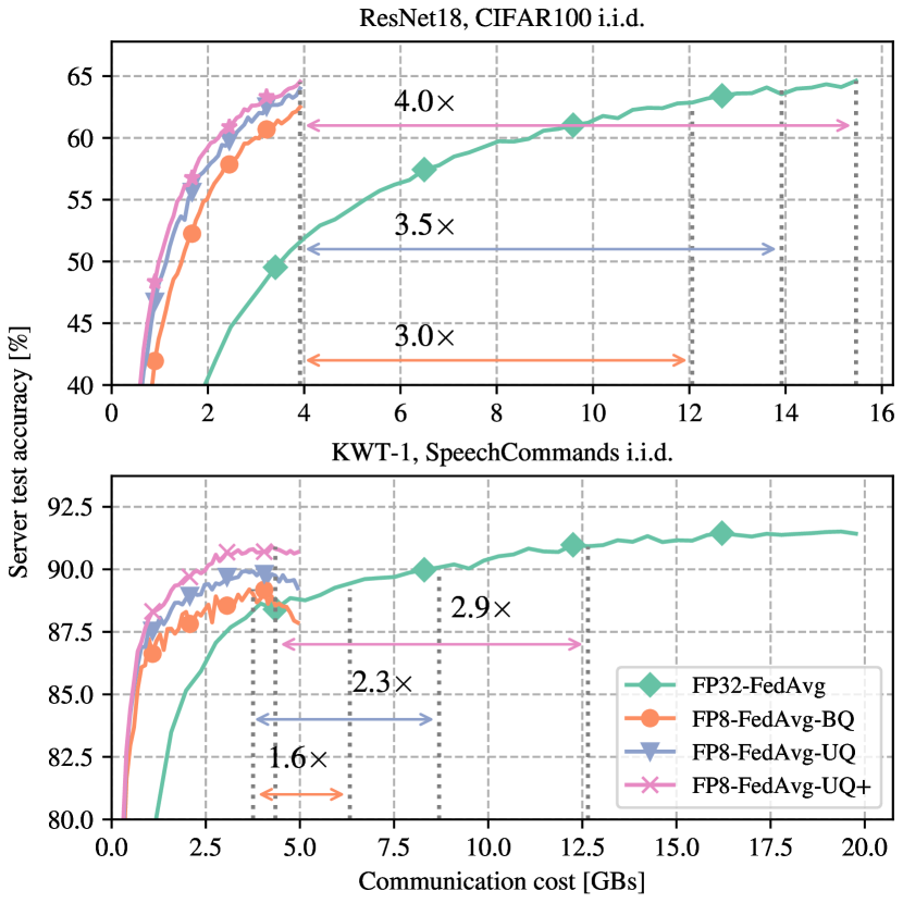
Results. The results are shown in Table 1, where we present the final centralized test accuracy as well as the communication gain for each model and dataset, with and without server-side optimization, across three random seeds. In order to compare communication costs, we do not pick a common accuracy threshold for all methods, but instead calculate the gains individually for each method as the reduction in communicated bytes compared to FP32 training at the maximum accuracy reached by both FP32 and FP8. In Table 1 it can be seen that for most datasets and methods, FP8-FedAvg-UQ achieves similar test accuracy as the FP32 baseline, which results in communication gains around 4x on average. Note that even though FP8 quantization sometimes results in a small accuracy drop, a large communication gain is still possible due to less data being transferred in each communication round. However, in certain cases, for example when applying FP8 quantization to LeNet on CIFAR100, accuracy increases significantly compared to the FP32 baseline. For these experiments, we observed that FP8 quantization to some extent prevented overfitting to the local client datasets, and thereby acted as a regularizer. This effect of quantization has been observed in other studies as well (AskariHemmat et al., 2022). Finally, we note that the server-side optimization in most scenarios yields additional performance improvements, which results in communication gains greater than 2.9x compared to FP32 across all tasks and models.

Ablation studies. Next, we ablate the use of deterministic and stochastic quantization in order to validate our design choices. Table 2 shows the server test accuracy when using the two different quantization methods for the on-device QAT training. Deterministic quantization works best here, which can also be understood intuitively, since in each forward pass through the network, deterministic quantization results in a smaller quantization error. We refer to Appendix B for more details about QAT convergence.

We also ablate the effect of deterministic and stochastic quantization in server-device communication, and it is clear that stochastic quantization results in both higher accuracy and gain. This is in agreement with Remark 3, which shows that stochastic quantization is important for the convergence of our algorithm. In addition, we show the server test accuracy as a function of communication cost for different methods in Figure 2. Here we can clearly see the gain arising from quantized communication, as well as the benefits of stochastic quantization and server-side optimization.

Table 2. Final test accuracy on CIFAR100 (i.i.d.) for deterministic/stochastic QAT and quantized communication (CQ).
FP8 QAT without CQ FP8 det. QAT with CQ
Model det. QAT rand. QAT det. CQ rand. CQ
LeNet $44.4\pm 0.5$ $43.7\pm 0.6$ $38.0\pm 0.4$ $44.8\pm 0.4$
ResNet18 $64.5\pm 0.1$ $63.5\pm 0.5$ $62.5\pm 0.9$ $64.0\pm 0.2$

5. Conclusions and Future Work

In this work, we show that on-device FP8 QAT training combined with quantized communication can be integrated into a federated learning setting with a well-designed algorithm. Our results show that this can be done with minimal drop in model predictive performance, while obtaining large savings in terms of communication cost. This opens up a wide range of possibilities in terms of exploiting client heterogeneity. For example, it allows for combining devices with different computational capabilities, which could involve training with different levels of precision in different clients. Furthermore, since the use of low-precision number formats is orthogonal to the optimization method itself, our proposed method may be extended beyond standard federated averaging. We leave this as future work and hope our work will inspire the wider research community to explore different combinations of floating point number formats in a federated learning setting.

Refer to caption
Figure 2. Server test accuracy versus communication cost for FP32 FedAvg, and FP8 QAT with biased (BQ)/unbiased (UQ) communication, and server-side optimization (UQ+).

References

  • (1)
  • Acar et al. (2021) Durmus Alp Emre Acar, Yue Zhao, Ramon Matas, Matthew Mattina, Paul Whatmough, and Venkatesh Saligrama. 2021. Federated Learning Based on Dynamic Regularization. In International Conference on Learning Representations. https://openreview.net/forum?id=B7v4QMR6Z9w
  • AskariHemmat et al. (2022) MohammadHossein AskariHemmat, Reyhane Askari Hemmat, Alex Hoffman, Ivan Lazarevich, Ehsan Saboori, Olivier Mastropietro, Sudhakar Sah, Yvon Savaria, and Jean-Pierre David. 2022. QReg: On regularization effects of quantization. arXiv preprint arXiv:2206.12372 (2022).
  • Bengio et al. (2013) Yoshua Bengio, Nicholas Léonard, and Aaron Courville. 2013. Estimating or propagating gradients through stochastic neurons for conditional computation. arXiv preprint arXiv:1308.3432 (2013).
  • Berg et al. (2021) Axel Berg, Mark O’Connor, and Miguel Tairum Cruz. 2021. Keyword Transformer: A Self-Attention Model for Keyword Spotting. In Proc. Interspeech 2021. 4249–4253. https://doi.org/10.21437/Interspeech.2021-1286
  • Beznosikov et al. (2023) Aleksandr Beznosikov, Samuel Horváth, Peter Richtárik, and Mher Safaryan. 2023. On biased compression for distributed learning. Journal of Machine Learning Research 24, 276 (2023), 1–50.
  • Bouzinis et al. (2023) Pavlos S Bouzinis, Panagiotis D Diamantoulakis, and George K Karagiannidis. 2023. Wireless quantized federated learning: a joint computation and communication design. IEEE Transactions on Communications (2023).
  • Gupta et al. (2023) Kartik Gupta, Marios Fournarakis, Matthias Reisser, Christos Louizos, and Markus Nagel. 2023. Quantization Robust Federated Learning for Efficient Inference on Heterogeneous Devices. TMLR (2023).
  • He et al. (2016) Kaiming He, Xiangyu Zhang, Shaoqing Ren, and Jian Sun. 2016. Deep residual learning for image recognition. In Proceedings of the IEEE conference on computer vision and pattern recognition. 770–778.
  • He et al. (2020) Yang He, Hui-Po Wang, Maximilian Zenk, and Mario Fritz. 2020. CosSGD: Communication-efficient federated learning with a simple cosine-based quantization. arXiv preprint arXiv:2012.08241 (2020).
  • Hönig et al. (2022) Robert Hönig, Yiren Zhao, and Robert Mullins. 2022. DAdaQuant: Doubly-adaptive quantization for communication-efficient Federated Learning. In International Conference on Machine Learning. PMLR, 8852–8866.
  • Hsieh et al. (2020) Kevin Hsieh, Amar Phanishayee, Onur Mutlu, and Phillip Gibbons. 2020. The non-iid data quagmire of decentralized machine learning. In International Conference on Machine Learning. PMLR, 4387–4398.
  • Karimireddy et al. (2020) Sai Praneeth Karimireddy, Satyen Kale, Mehryar Mohri, Sashank Reddi, Sebastian Stich, and Ananda Theertha Suresh. 2020. Scaffold: Stochastic controlled averaging for federated learning. In International conference on machine learning. PMLR, 5132–5143.
  • Krizhevsky (2009) Alex Krizhevsky. 2009. Learning multiple layers of features from tiny images. Technical Report.
  • Kuzmin et al. (2022) Andrey Kuzmin, Mart Van Baalen, Yuwei Ren, Markus Nagel, Jorn Peters, and Tijmen Blankevoort. 2022. Fp8 quantization: The power of the exponent. Advances in Neural Information Processing Systems 35 (2022), 14651–14662.
  • Li et al. (2017) Hao Li, Soham De, Zheng Xu, Christoph Studer, Hanan Samet, and Tom Goldstein. 2017. Training quantized nets: A deeper understanding. Advances in Neural Information Processing Systems 30 (2017).
  • Li et al. (2022) Xin-Chun Li, Jin-Lin Tang, Shaoming Song, Bingshuai Li, Yinchuan Li, Yunfeng Shao, Le Gan, and De-Chuan Zhan. 2022. Avoid Overfitting User Specific Information in Federated Keyword Spotting. In Proc. Interspeech 2022. 3869–3873. https://doi.org/10.21437/Interspeech.2022-558
  • Loshchilov and Hutter (2018) Ilya Loshchilov and Frank Hutter. 2018. Decoupled Weight Decay Regularization. In International Conference on Learning Representations.
  • Majumdar and Ginsburg (2020) Somshubra Majumdar and Boris Ginsburg. 2020. MatchboxNet: 1D Time-Channel Separable Convolutional Neural Network Architecture for Speech Commands Recognition. In Proc. Interspeech 2020. 3356–3360. https://doi.org/10.21437/Interspeech.2020-1058
  • McMahan et al. (2017) Brendan McMahan, Eider Moore, Daniel Ramage, Seth Hampson, and Blaise Aguera y Arcas. 2017. Communication-efficient learning of deep networks from decentralized data. In Artificial intelligence and statistics. PMLR, 1273–1282.
  • Micikevicius et al. (2022) Paulius Micikevicius, Dusan Stosic, Neil Burgess, Marius Cornea, Pradeep Dubey, Richard Grisenthwaite, Sangwon Ha, Alexander Heinecke, Patrick Judd, John Kamalu, et al. 2022. Fp8 formats for deep learning. arXiv:2209.05433 (2022).
  • Nesterov et al. ([n. d.]) Yurii Nesterov et al. [n. d.]. Lectures on convex optimization. Vol. 137. Springer.
  • Ni et al. (2024) Renkun Ni, Yonghui Xiao, Phoenix Meadowlark, Oleg Rybakov, Tom Goldstein, Ananda Theertha Suresh, Ignacio Lopez Moreno, Mingqing Chen, and Rajiv Mathews. 2024. FedAQT: Accurate Quantized Training with Federated Learning. In ICASSP 2024-2024 IEEE International Conference on Acoustics, Speech and Signal Processing (ICASSP). IEEE, 6100–6104.
  • Park et al. (2019) Daniel S. Park, William Chan, Yu Zhang, Chung-Cheng Chiu, Barret Zoph, Ekin D. Cubuk, and Quoc V. Le. 2019. SpecAugment: A Simple Data Augmentation Method for Automatic Speech Recognition. In Proc. Interspeech 2019. 2613–2617. https://doi.org/10.21437/Interspeech.2019-2680
  • Peng et al. (2023) Houwen Peng, Kan Wu, Yixuan Wei, Guoshuai Zhao, Yuxiang Yang, Ze Liu, Yifan Xiong, Ziyue Yang, Bolin Ni, Jingcheng Hu, et al. 2023. Fp8-lm: Training fp8 large language models. arXiv preprint arXiv:2310.18313 (2023).
  • Richtárik et al. (2021) Peter Richtárik, Igor Sokolov, and Ilyas Fatkhullin. 2021. EF21: A new, simpler, theoretically better, and practically faster error feedback. Advances in Neural Information Processing Systems 34 (2021), 4384–4396.
  • Sun et al. (2019) Xiao Sun, Jungwook Choi, Chia-Yu Chen, Naigang Wang, Swagath Venkataramani, Vijayalakshmi Viji Srinivasan, Xiaodong Cui, Wei Zhang, and Kailash Gopalakrishnan. 2019. Hybrid 8-bit floating point (HFP8) training and inference for deep neural networks. NeurIPS 32 (2019).
  • Vishwanath (2019) Amulya Vishwanath. 2019. Mixed-Precision Training Techniques Using Tensor Cores for Deep Learning. https://developer.nvidia.com/blog/video-mixed-precision-techniques-tensor-cores-deep-learning/. Accessed: 2019-01-30.
  • Wang et al. (2018) Naigang Wang, Jungwook Choi, Daniel Brand, Chia-Yu Chen, and Kailash Gopalakrishnan. 2018. Training deep neural networks with 8-bit floating point numbers. Advances in neural information processing systems 31 (2018).
  • Warden (2018) Pete Warden. 2018. Speech commands: A dataset for limited-vocabulary speech recognition. arXiv preprint arXiv:1804.03209 (2018).
  • Wu and He (2018) Yuxin Wu and Kaiming He. 2018. Group normalization. In Proceedings of the European conference on computer vision (ECCV). 3–19.
  • Youn et al. (2023) Yeojoon Youn, Zihao Hu, Juba Ziani, and Jacob Abernethy. 2023. Randomized Quantization is All You Need for Differential Privacy in Federated Learning. In Federated Learning and Analytics in Practice: Algorithms, Systems, Applications, and Opportunities.
  • Zheng et al. (2020) Sihui Zheng, Cong Shen, and Xiang Chen. 2020. Design and analysis of uplink and downlink communications for federated learning. IEEE Journal on Selected Areas in Communications 39, 7 (2020), 2150–2167.

Appendix

For FedAvg convergence proof, our analysis builds on (Karimireddy et al., 2020; Li et al., 2017; Acar et al., 2021). (Karimireddy et al., 2020; Acar et al., 2021) focus on debiasing the local losses in a standard non-quantized federated learning setting. Differently, we show convergence using quantization aware training in federated learning. We can further extend our analysis to use the sophisticated debiasing methods for better heterogeneity control. Li et al. (2017) proves convergence of different quantization aware training schemes in a centralized non-federated setting. Differently, we give convergence of quantization aware training in a distributed federated learning setting. Additionally, we give a proof for more general non-uniform quantization grids such as FP8, which is different from the uniform quantization consideration in (Li et al., 2017).

Appendix A Quantization Function

Definition 0 (Quantization).

For an unquantized number $x$, we define the quantization of $x$ as

$\displaystyle Q_{\text{rand}}(x)=s\begin{cases}\left\lceil\frac{x}{s}\right\rceil&p\leq\frac{x}{s}-\left\lfloor\frac{x}{s}\right\rfloor\\ \left\lfloor\frac{x}{s}\right\rfloor&\text{otherwise,}\end{cases},\ \ \ \ Q_{\text{det}}({x})=s\left\lfloor\frac{x}{s}\right\rceil,$

where $p\in[0,1]$ is a random variable. We omit the parameter of quantization for the sake of simplicity in the notation. We overload the notation and define quantization of a vector $\mathbf{x}\in\mathbb{R}^{d}$ as the element-wise quantization of the vector, $Q({\mathbf{x}})=\left[Q\left(\left[{\mathbf{x}}\right]_{1}\right),Q\left(\left[{\mathbf{x}}\right]_{2}\right),\ldots,Q\left(\left[{\mathbf{x}}\right]_{d}\right)\right]^{T}$

Let’s define the quantization error.

Definition 0 (Quantization Error).

Let $r_{Q}\left(\mathbf{w}\right)=Q\left(\mathbf{w}\right)-\mathbf{w}$.

Note that if $Er_{Q}\left(\mathbf{w}\right)=\mathbf{0}$, we have an unbiased quantization as in our model transmission where expectation is over the randomness of the quantization.

Note that we simplified the definition by ignoring the quantization based learnable parameters such as $\alpha$ and $\beta$ in our proof. Hence, we redefine them here.

Appendix B Convergence Analysis of Quantization-aware Training (QAT)

As a warmup, we provide the convergence analysis of QAT training on a single machine, similar to the one in (Li et al., 2017).

We want to find a quantized model that solves $\min_{\mathbf{w\in\mathbb{R}^{d}}}F(\mathbf{w})$. We start with an unquantized model as $\mathbf{w}_{1}$ and use QAT training as $\mathbf{w}_{t+1}=\mathbf{w}_{t}-\eta_{t}\nabla F\left(Q\left(\mathbf{w}_{t}\right);\xi_{t}\right)$ where $\eta_{t}$ is learning rate and $\xi_{t}$ controls randomness of SGD at iterate $t$. Let us define the best model as $\mathbf{w}_{*}=\arg\min_{\mathbf{w}}F(\mathbf{w})$.

Our analysis is based on the following assumptions on the objective function $F$.

Assumption 1 (Convexity).

We assume that $F$ is differentiable and convex, i.e.,

$$-\left\langle\nabla F({\mathbf{x}}),{\mathbf{x}}-{\mathbf{y}}\right\rangle\leq-F({\mathbf{x}})+F({\mathbf{y}})\ \ \ \forall{\mathbf{x}},{\mathbf{y}}.$$
Assumption 2 (Bounded Unbiased Gradients).

We assume the gradients are unbiased and bounded.

$$E_{\xi}[\nabla F\left(\mathbf{x};\xi\right)]=\nabla F\left(\mathbf{x}\right),\ \ E_{\xi}\|\nabla F\left(\mathbf{x};\xi\right)\|^{2}_{2}\leq G^{2}\ \ \ \forall{\mathbf{x}}.$$

where $\xi$ defines the randomness due to stochastic gradient estimator. The algorithm draws $\nabla F\left(\mathbf{x};\xi\right)$ instead of $\nabla F\left(\mathbf{x}\right)$.

Assumption 3 (Bounded Quantization Scales).

We assume the scales $s_{i}$ are uniformly upper bounded during the training by a constant $S$.

Next, we provide an upper bound on the quantization error.

Lemma 0.

If assumption 3 holds, we have,

$$E\|r_{Q}\left({\mathbf{w}}\right)\|_{2}\leq\sqrt{d}S$$
Proof.

Each dimension of $r_{Q}\left({\mathbf{w}}\right)$ can be at max $S$. We have $d$ dimensions. Hence, $E\|r_{Q}\left({\mathbf{w}}\right)\|_{2}\leq\sqrt{d}S$

We can then prove the following lemma on the $t$-th iteration of QAT training.

Lemma 0 (QAT step update).

If assumptions 1, 2, and 3 hold and $\eta_{t}=\frac{1}{\sqrt{T}}$, we have,

$$E\left[F\left(Q\left(\mathbf{w}_{t}\right)\right)-F\left(\mathbf{w}_{*}\right)\right]\leq\frac{\sqrt{T}}{2}\left[-E\|\mathbf{w}_{t+1}-\mathbf{w}_{*}\|^{2}_{2}+E\|\mathbf{w}_{t}-\mathbf{w}_{*}\|^{2}_{2}\right]+G\sqrt{d}S+\frac{1}{2\sqrt{T}}G^{2}$$
Proof.

Based on the update $\mathbf{w}_{t+1}=\mathbf{w}_{t}-\eta_{t}\nabla F\left(Q\left(\mathbf{w}_{t}\right);\xi_{t}\right)$ in the $t$-th iteration of QAT training,

$\displaystyle E\|\mathbf{w}_{t+1}-\mathbf{w}_{*}\|_{2}^{2}$ $\displaystyle=E\|\mathbf{w}_{t}-\eta_{t}\nabla F\left(Q\left(\mathbf{w}_{t}\right);\xi_{t}\right)-\mathbf{w}_{*}\|^{2}_{2}$
$\displaystyle=E\|\mathbf{w}_{t}-\mathbf{w}_{*}\|^{2}_{2}-2\eta_{t}E\left\langle\nabla F\left(Q\left(\mathbf{w}_{t}\right);\xi_{t}\right),\mathbf{w}_{t}-\mathbf{w}_{*}\right\rangle+\eta_{t}^{2}E\|\nabla F\left(Q\left(\mathbf{w}_{t}\right);\xi_{t}\right)\|^{2}_{2}$
$\displaystyle\leq E\|\mathbf{w}_{t}-\mathbf{w}_{*}\|^{2}_{2}-2\eta_{t}E\left\langle\nabla F\left(Q\left(\mathbf{w}_{t}\right);\xi_{t}\right),\mathbf{w}_{t}-\mathbf{w}_{*}\right\rangle+\eta_{t}^{2}G^{2}$
$\displaystyle=E\|\mathbf{w}_{t}-\mathbf{w}_{*}\|^{2}_{2}-2\eta_{t}E\left\langle\nabla F\left(Q\left(\mathbf{w}_{t}\right)\right),\mathbf{w}_{t}-\mathbf{w}_{*}\right\rangle+\eta_{t}^{2}G^{2}$
$\displaystyle=E\|\mathbf{w}_{t}-\mathbf{w}_{*}\|^{2}_{2}-2\eta_{t}E\left\langle\nabla F\left(Q\left(\mathbf{w}_{t}\right)\right),Q\left(\mathbf{w}_{t}\right)-\mathbf{w}_{*}\right\rangle-2\eta_{t}E\left\langle\nabla F\left(Q\left(\mathbf{w}_{t}\right)\right),\mathbf{w}_{t}-Q\left(\mathbf{w}_{t}\right)\right\rangle+\eta_{t}^{2}G^{2}$
$\displaystyle\leq E\|\mathbf{w}_{t}-\mathbf{w}_{*}\|^{2}_{2}-2\eta_{t}E\left(F\left(Q\left(\mathbf{w}_{t}\right)\right)-F\left(\mathbf{w}_{*}\right)\right)-2\eta_{t}E\left\langle\nabla F\left(Q\left(\mathbf{w}_{t}\right)\right),\mathbf{w}_{t}-Q\left(\mathbf{w}_{t}\right)\right\rangle+\eta_{t}^{2}G^{2}$
$\displaystyle\leq E\|\mathbf{w}_{t}-\mathbf{w}_{*}\|^{2}_{2}-2\eta_{t}E\left(F\left(Q\left(\mathbf{w}_{t}\right)\right)-F\left(\mathbf{w}_{*}\right)\right)+2\eta_{t}E\left\|\nabla F\left(Q\left(\mathbf{w}_{t}\right)\right)\right\|_{2}\left\|r\left(\mathbf{w}_{t}\right)\right\|_{2}+\eta_{t}^{2}G^{2}$
$\displaystyle\leq E\|\mathbf{w}_{t}-\mathbf{w}_{*}\|^{2}_{2}-2\eta_{t}E\left(F\left(Q\left(\mathbf{w}_{t}\right)\right)-F\left(\mathbf{w}_{*}\right)\right)+2\eta_{t}GE\left\|r\left(\mathbf{w}_{t}\right)\right\|_{2}+\eta_{t}^{2}G^{2}$
$\displaystyle\leq E\|\mathbf{w}_{t}-\mathbf{w}_{*}\|^{2}_{2}-2\eta_{t}E\left(F\left(Q\left(\mathbf{w}_{t}\right)\right)-F\left(\mathbf{w}_{*}\right)\right)+2\eta_{t}G\sqrt{d}S+\eta_{t}^{2}G^{2}$

where A.2, A.1, $\langle\mathbf{x},\mathbf{y}\rangle\leq\|\mathbf{x}\|_{2}\|\mathbf{y}\|_{2}$, A.2, and Lemma B.1 are used respectively in the inequalities. We use the fact that gradients are unbiased as well, A.2. Let $\eta_{t}=\frac{1}{\sqrt{T}}$. Note that the same rate can be obtained with a decreasing learning rate scheme with a couple extra steps. Rearranging the terms and dividing with the learning rate give the Lemma. ∎

By the telescoping sum of Lemma B.2 over all iterations $t=1,\dotsc,T$, we can prove the convergence of QAT training.

Theorem B.3 (QAT Convergence).

For a convex function with bounded unbiased stochastic gradients using a quantization method with bounded scales, we have

$$E\left[F\left(Q\left(\mathbf{w}_{\tau}\right)\right)-F\left(\mathbf{w}_{*}\right)\right]=O\left(\frac{1}{\sqrt{T}}\left(\|\mathbf{w}_{1}-\mathbf{w}_{*}\|^{2}_{2}+G^{2}\right)+G\sqrt{d}S\right)$$

where $\tau$ is a random variable that takes values in $\{1,2,\ldots,T\}$ with equal probability111We could further derive a model bound using Jensen on LHS since the function is convex. This allows us to avoid introducing another random variable $\tau$, and would give LHS as $E\left[F\left(\frac{1}{T}\sum_{t=1}^{T}Q\left(\mathbf{w}_{t}\right)\right)-F\left(\mathbf{w}_{*}\right)\right]$. However the model, $\frac{1}{T}\sum_{t=1}^{T}Q\left(\mathbf{w}_{t}\right)$, is not necessarily a quantized model. Since we are interested in quantized model performance, we further need to argue that the quantization error of the averaged model is small and that would not change the rate. To avoid these extra steps, we introduced another random variable, $\tau$, for the sake of simplicity in the proof., $T$ is the number of iterations, $\mathbf{w}_{1}$ is the initial model and $\mathbf{w}_{*}$ is the optimal model $\mathbf{w}_{*}\in\arg\min_{\mathbf{w}}F(\mathbf{w})$, and the remaining constants are defined in the assumptions.

Proof.

If we average Lemma B.2 for all iterations we get,

$\displaystyle E\left[\left[\frac{1}{T}\sum_{t=1}^{T}F\left(Q\left(\mathbf{w}_{t}\right)\right)\right]-F\left(\mathbf{w}_{*}\right)\right]$ $\displaystyle\leq\frac{1}{2\sqrt{T}}\left[-E\|\mathbf{w}_{T+1}-\mathbf{w}_{*}\|^{2}_{2}+E\|\mathbf{w}_{1}-\mathbf{w}_{*}\|^{2}_{2}\right]+G\sqrt{d}S+\frac{1}{2\sqrt{T}}G^{2}$
$\displaystyle\leq\frac{1}{2\sqrt{T}}\|\mathbf{w}_{1}-\mathbf{w}_{*}\|^{2}_{2}+G\sqrt{d}S+\frac{1}{2\sqrt{T}}G^{2}$

Note that LHS is the same if we choose $Q\left(\mathbf{w}_{t}\right)$ at random from all iterations with equal probability. ∎

Remark 5.

Note that the proof uses a bound on the quantization error in the form of Lemma B.1. Deterministic quantization would have a smaller bound on the norm of the quantization error, $E\left\|r_{Q}(w)\right\|_{2}$, compared to the stochastic quantization. This motivates the use of deterministic quantization during the training phase.

Remark 6.

LHS of the convergence rate in Theorem B.3 has two terms. First term decays with $O\left(\frac{1}{\sqrt{T}}\right)$ which is similar to the SGD rate. The second term is a constant. This constant term accounts for irreducible loss due to quantization.

Appendix C Convergence Analysis of FP8FedAvg-UQ

We note that $F_{k}$ is the local loss at device $k\in[K]$ and $F$ is the average of local functions, .i.e $F\left(\mathbf{x}\right)=\frac{1}{K}\sum_{k=1}^{K}F_{k}\left(\mathbf{w}\right)$. We assume the number of data points in each device is the same so that $F$ is a non-weighted average of local functions for the sake of simplicity. We note that results can be adjusted easily for non-equal dataset size cases. We denote $\mathbf{w}^{*}$ as the optimal model of the global loss, .i.e $\arg\min F\left(\mathbf{w}\right)$. For simplicity, we consider the balanced clients $n_{k}=\frac{n}{K}$ in our proof. However, the proof can be extended to the general imbalanced case similar to (McMahan et al., 2017).

Assumption 4 (Smoothness).

We assume the functions are $L$ smooth.

$$\|\nabla F_{k}({\mathbf{x}})-\nabla F_{k}({\mathbf{y}})\|_{2}\leq L\|{\mathbf{x}}-{\mathbf{y}}\|_{2}\ \ \ \forall{\mathbf{x}},{\mathbf{y}},k.$$
Property 1.

If we have smooth and convex functions, as in (Karimireddy et al., 2020; Nesterov et al., [n. d.]; Acar et al., 2021), for all $\mathbf{w},\mathbf{x},\mathbf{y}$,

$$-\left\langle\nabla F_{k}\left(\mathbf{w}\right),\mathbf{y}-\mathbf{x}\right\rangle\leq-F_{k}\left(\mathbf{y}\right)+F_{k}\left(\mathbf{x}\right)+\frac{L}{2}\left\|\mathbf{y}-\mathbf{w}\right\|^{2}_{2}.$$

C.1. Lemmas on the Stochastic Quantization for Model Communication

Lemma 0.

Stochastic quantization is unbiased, i.e.,

$$Er_{Q_{\text{rand}}}\left(\mathbf{x}\right)=\mathbf{0}.$$
Proof.

It follows directly from the definition as,

$\displaystyle Er_{Q_{\text{rand}}}\left(\mathbf{x}\right)$ $\displaystyle=EQ_{\text{rand}}\left(\mathbf{x}\right)-\mathbf{x}=s\left(\frac{{\mathbf{x}}}{s}-\left\lfloor\frac{{\mathbf{x}}}{s}\right\rfloor\right)\odot\left(\left\lfloor\frac{{\mathbf{x}}}{s}\right\rfloor+1\right)+s\left(1-\frac{{\mathbf{x}}}{s}+\left\lfloor\frac{{\mathbf{x}}}{s}\right\rfloor\right)\odot\left\lfloor\frac{{\mathbf{x}}}{s}\right\rfloor-\mathbf{x}=\mathbf{0}$

where $\odot$ denotes the element-wise product. ∎

Lemma 0.

Let $Q_{\text{rand}}$ be the stochastic unbiased quantization satisfying assumption 3 . Then we have,

$$E\left\|r_{Q_{\text{rand}}}\left({\mathbf{x}}\right)\right\|^{2}_{2}\leq S\left\|{\mathbf{x}}\right\|_{1}\leq S\sqrt{d}\left\|{\mathbf{x}}\right\|_{2}$$
Proof.

Let’s start with a scalar case and we extend it to a vector case.

$\displaystyle E\left|r_{Q_{\text{rand}}}\left({x}\right)\right|^{2}$ $\displaystyle=s^{2}\left(\frac{x}{s}-\left\lfloor\frac{x}{s}\right\rfloor\right)\left(\left\lfloor\frac{x}{s}\right\rfloor+1-\frac{x}{s}\right)^{2}+s^{2}\left(1-\frac{x}{s}+\left\lfloor\frac{x}{s}\right\rfloor\right)\left(\left\lfloor\frac{x}{s}\right\rfloor-\frac{x}{s}\right)^{2}$
$\displaystyle=s^{2}\left(\frac{x}{s}-\left\lfloor\frac{x}{s}\right\rfloor\right)\left(1+\left\lfloor\frac{x}{s}\right\rfloor-\frac{x}{s}\right)\leq s^{2}\min\left(\frac{x}{s}-\left\lfloor\frac{x}{s}\right\rfloor,1-\frac{x}{s}+\left\lfloor\frac{x}{s}\right\rfloor\right)$
$\displaystyle\leq s^{2}\left|\frac{x}{s}\right|\leq S|x|$

where inequalities follow from the fact that $\frac{x}{s}-\left\lfloor\frac{x}{s}\right\rfloor\leq 1$.

We can add the scalar variances to bound a vector variance as,

$\displaystyle E\left\|r_{Q_{\text{rand}}}\left({\mathbf{x}}\right)\right\|^{2}_{2}=\sum_{i\in[d]}E\left\|r_{Q_{\text{rand}}}\left(\left[{\mathbf{x}}\right]_{i}\right)\right\|^{2}_{2}\leq S\sum_{i\in[d]}\left|\left[{\mathbf{x}}\right]_{i}\right|=S\left\|{\mathbf{x}}\right\|_{1}\leq S\sqrt{d}\left\|{\mathbf{x}}\right\|_{2}$

where we use Cauchy–Schwarz inequality in the last step.

Lemma 0 (Quantization Error Decomposition).

Let assumption 3 holds. Both uniform and FP8 quantization satisfies,

$$E\left|r_{Q}\left(Q\left({x}\right)+{y}\right)\right|^{2}\leq S\left|{y}\right|.$$

For $d$ dimensional vectors we get,

$$E\left\|r_{Q}\left(Q\left(\mathbf{x}\right)+\mathbf{y}\right)\right\|^{2}_{2}\leq S\sqrt{d}\left\|\mathbf{y}\right\|_{2}.$$
Proof.

We give a proof for scalar case. Vector version comes from upper bounding scalar case using Cauchy-Schwarz. Note that variance is higher for randomized quantization so let’s prove the bound for $Q_{\text{rand}}$. Due to symmetry, we can assume $Q_{\text{rand}}\left({x}\right)\geq{0}$.

Let’s define grid points as $g_{i}$ where $g_{0}=0$ and $g_{i+1}>g_{i}$. Note that due to quantization definitions, we have $g_{i}\%(g_{i+1}-g_{i})=0$, .i.e $\exists k\in\mathcal{Z}^{+}$ such that $g_{i}=k\left(g_{i+1}-g_{i}\right)$. Furthermore, we have a finer resolution close to 00, .i.e $g_{i+1}-g_{i}\geq g_{i}-g_{i-1}$.

We extensively use a step in Lemma C.2 as,

$$E\left|r_{Q_{\text{rand}}}\left(z\right)\right|^{2}=s^{2}q_{z}\left(1-q_{z}\right)\leq s^{2}\min\left(q_{z},1-q_{z}\right)\leq s^{2}\left|\frac{z}{s}\right|=s|z|$$

where $q_{z}=\frac{z}{s}-\left\lfloor\frac{z}{s}\right\rfloor$. We use this relation by plugging in $z=Q_{\text{rand}}\left({x}\right)+y$ and investigating $q_{Q_{\text{rand}}\left({x}\right)+y}$.

Since $Q_{\text{rand}}\left({x}\right)$ is already quantized, $\exists i\geq 0$ such that $Q_{\text{rand}}\left({x}\right)=g_{i}$. Let $g_{j+1}>Q_{\text{rand}}\left({x}\right)+y\geq g_{j}$.

Let $y=\delta+g_{j}-g_{i}$. Then we have $g_{j+1}>\delta+g_{j}\geq g_{j}\implies g_{j+1}-g_{j}>\delta\geq 0$. We also know $g_{j+1}-g_{i}>y\geq g_{j}-g_{i}$.

We have, by definition,

$$q_{Q_{\text{rand}}\left({x}\right)+y}=\frac{g_{j}+\delta}{g_{j+1}-g_{j}}-\left\lfloor\frac{g_{j}+\delta}{g_{j+1}-g_{j}}\right\rfloor=\frac{\delta}{g_{j+1}-g_{j}}-\left\lfloor\frac{\delta}{g_{j+1}-g_{j}}\right\rfloor=q_{\delta}$$

since $g_{j}$ is a multiple $g_{j+1}-g_{j}$.

Let’s look at different cases.

Case $i\leq j$

Note that $g_{j}-g_{i}\geq 0$ so that $|y|=|\delta+g_{j}-g_{i}|\geq|\delta|$. Then, we have,

$$E\left|r_{Q_{\text{rand}}}\left(Q\left({x}\right)+y\right)\right|^{2}\leq\left(g_{j+1}-g_{j}\right)^{2}\min\left(q_{\delta},1-q_{\delta}\right)\leq\left(g_{j+1}-g_{j}\right)|\delta|\leq S|\delta|\leq S|y|\qed.$$

Case $i>j+1$

Note that $g_{j+1}-g_{i}<0$ and $y$ is negative. Let’s look at magnitude of $y$ and $\delta$.

$$0>g_{j+1}-g_{i}>y\geq g_{j}-g_{i}\implies|y|>g_{i}-g_{j+1}\geq g_{j+2}-g_{j+1}.$$

We already know that $g_{j+1}-g_{j}>\delta\geq 0$. Then we have,

$$|y|>g_{j+2}-g_{j+1}\geq g_{j+1}-g_{j}>\delta$$

Since $|y|>|\delta|$, we get,

$$E\left|r_{Q_{\text{rand}}}\left(Q\left({x}\right)+y\right)\right|^{2}\leq\left(g_{j+1}-g_{j}\right)^{2}\min\left(q_{\delta},1-q_{\delta}\right)\leq\left(g_{j+1}-g_{j}\right)|\delta|\leq S|\delta|\leq S|y|\qed.$$

Case $i=j+1$

We have $y=\delta+g_{j}-g_{i}=\delta-\left(g_{j+1}-g_{j}\right)$. Let’s look at $q_{\delta}$ as,

$$q_{\delta}=\frac{\delta}{g_{j+1}-g_{j}}-\left\lfloor\frac{\delta}{g_{j+1}-g_{j}}\right\rfloor=\frac{\delta-\left(g_{j+1}-g_{j}\right)}{g_{j+1}-g_{j}}-\left\lfloor\frac{\delta-\left(g_{j+1}-g_{j}\right)}{g_{j+1}-g_{j}}\right\rfloor=\frac{y}{g_{j+1}-g_{j}}-\left\lfloor\frac{y}{g_{j+1}-g_{j}}\right\rfloor=q_{y}$$

Then we have,

$$E\left|r_{Q_{\text{rand}}}\left(Q\left({x}\right)+y\right)\right|^{2}\leq\left(g_{j+1}-g_{j}\right)^{2}\min\left(q_{\delta},1-q_{\delta}\right)=\left(g_{j+1}-g_{j}\right)^{2}\min\left(q_{y},1-q_{y}\right)\leq\left(g_{j+1}-g_{j}\right)|y|\leq S|y|.$$

Please note that the above proof holds for any quantization scheme of which the grid is symmetric with respect to zero and the bin size increases monotonically going from zero to plus or minus infinity. The FP8 quantization obviously satisfies this condition.

C.2. Lemma on a Single Communication Round

We define some useful quantities. For simplicity in the proof, let us define auxiliary models as,

$${\mathbf{v}}_{t,u+1}^{k}={\mathbf{v}}_{t,u}^{k}-\eta_{t}\nabla F_{k}\left(Q_{\text{det}}\left({\mathbf{v}}_{t,u}^{k}\right);\xi_{t,u}^{k}\right)\ \ \forall u\in[U],\ \ \ \ {\mathbf{v}}_{t,1}^{k}=Q_{\text{rand}}\left({\mathbf{w}}_{t}\right)$$

where $U$ is the total number of local updates per communication round per device. Furthermore, we can unroll the recursion as,

$\displaystyle{\mathbf{v}}_{t,U+1}^{k}$ $\displaystyle={\mathbf{v}}_{t,U}^{k}-\eta_{t}\nabla F_{k}\left(Q_{\text{det}}\left({\mathbf{v}}_{t,U}^{k}\right);\xi_{t,U}^{k}\right)={\mathbf{v}}_{t,UE-1}^{k}-\eta_{t}\nabla F_{k}\left(Q_{\text{det}}\left({\mathbf{v}}_{t,U-1}^{k}\right);\xi_{t,U-1}^{k}\right)-\eta_{t}\nabla F_{k}\left(Q_{\text{det}}\left({\mathbf{v}}_{t,U}^{k}\right);\xi_{t,U}^{k}\right)=\ldots$
$\displaystyle=Q_{\text{rand}}\left({\mathbf{w}}_{t}\right)-\eta_{t}\sum_{u\in[U]}\nabla F_{k}\left(Q_{\text{det}}\left({\mathbf{v}}_{t,u}^{k}\right);\xi_{t,u}^{k}\right)$

It is clear to see that ${\mathbf{w}}_{t+1}^{k}={\mathbf{v}}_{t,U+1}^{k}$ for active devices. Let’s define inactive device ${\mathbf{w}}_{t+1}^{k}={\mathbf{v}}_{t,U+1}^{k}$ as well. Note that this is just for notation and the algorithm is unchanged. Because if $k$ is not active we do not use ${\mathbf{w}}_{t+1}^{k}$ in our algorithm. Let us define a drift quantity similar to (Karimireddy et al., 2020).

(6) $\displaystyle V_{t}=\frac{1}{KU}\sum_{k\in[K]}\sum_{u\in[U]}E\left\|Q_{\text{rand}}\left({\mathbf{w}}_{t}\right)-Q_{\text{det}}\left({\mathbf{v}}_{t,u}^{k}\right)\right\|^{2}_{2}.$

Note that if local models diverge, we get a higher $V_{t}$. We can obtain the following lemma for a single communication round of the FP8FedAvg-UQ algorithm.

Lemma 0.

If assumptions 1, 2, 3, 4 hold and we use an unbiased quantization for model transmission, we have,

(7) $\displaystyle E\|\mathbf{w}_{t+1}-\mathbf{w}_{*}\|^{2}_{2}$ $\displaystyle\leq E\left\|{\mathbf{w}}_{t}-\mathbf{w}_{*}\right\|^{2}_{2}-2U\eta_{t}E\left(F\left(Q_{\text{rand}}\left({\mathbf{w}}_{t}\right)\right)-F\left(\mathbf{w}_{*}\right)\right)+\eta_{t}LUV_{t}+2S\sqrt{d}GU\eta_{t}+\eta_{t}^{2}U^{2}G^{2}$
(8) $\displaystyle V_{t}$ $\displaystyle\leq 18U^{3}S\sqrt{d}G\eta_{t}+9U^{2}\eta_{t}^{2}G^{2}$
Proof.

First, we prove Eq. 7. Due to the model-to-server communication and the model aggregation on the server in the $t$-th round, we have

$\displaystyle E\left\|\mathbf{w}_{t+1}-\mathbf{w}_{*}\right\|^{2}_{2}=$ $\displaystyle E\left\|\frac{1}{P}\sum_{k\in\mathcal{P}_{t}}Q_{\text{rand}}\left({\mathbf{w}}_{t+1}^{k}\right)-\mathbf{w}_{*}\right\|^{2}_{2}\leq\frac{1}{P}E\sum_{k\in\mathcal{P}_{t}}\left\|Q_{\text{rand}}\left({\mathbf{w}}_{t+1}^{k}\right)-\mathbf{w}_{*}\right\|^{2}_{2}=\frac{1}{K}\sum_{k\in[K]}E\left\|Q_{\text{rand}}\left({\mathbf{w}}_{t+1}^{k}\right)-\mathbf{w}_{*}\right\|^{2}_{2}$

where we use definition of $\mathbf{w}_{t+1}$ and triangular inequality ($\left\|\sum_{n\in[N]}a_{n}\right\|^{2}\leq N\sum_{n\in[N]}\left\|a_{n}\right\|^{2}$). Lastly, we use the fact that active devices are sampled uniformly at random so that each device has an activation probability of $\frac{P}{K}$. Let’s continue as

$\displaystyle E\left\|\mathbf{w}_{t+1}-\mathbf{w}_{*}\right\|^{2}_{2}\leq$ $\displaystyle\frac{1}{K}\sum_{k\in[K]}E\left\|Q_{\text{rand}}\left({\mathbf{w}}_{t+1}^{k}\right)-\mathbf{w}_{*}\right\|^{2}_{2}=\frac{1}{K}\sum_{k\in[K]}E\left\|r_{Q_{\text{rand}}}\left({\mathbf{w}}_{t+1}^{k}\right)+{\mathbf{w}}_{t+1}^{k}-\mathbf{w}_{*}\right\|^{2}_{2}$
$\displaystyle=$ $\displaystyle\frac{1}{K}\left(\sum_{k\in[K]}E\left\|r_{Q_{\text{rand}}}\left({\mathbf{w}}_{t+1}^{k}\right)\right\|^{2}_{2}+2E\left\langle r_{Q_{\text{rand}}}\left({\mathbf{w}}_{t+1}^{k}\right),{\mathbf{w}}_{t+1}^{k}-\mathbf{w}_{*}\right\rangle+E\left\|{\mathbf{w}}_{t+1}^{k}-\mathbf{w}_{*}\right\|^{2}_{2}\right)$
$\displaystyle=$ $\displaystyle\frac{1}{K}\left(\sum_{k\in[K]}E\left\|r_{Q_{\text{rand}}}\left({\mathbf{w}}_{t+1}^{k}\right)\right\|^{2}_{2}+E\left\|{\mathbf{w}}_{t+1}^{k}-\mathbf{w}_{*}\right\|^{2}_{2}\right)$

where we use the fact that $Q_{\text{rand}}$ is an unbiased quantizer. Let’s bound $E\left\|{\mathbf{w}}_{t+1}^{k}-\mathbf{w}_{*}\right\|^{2}$ as

$\displaystyle E\left\|{\mathbf{w}}_{t+1}^{k}-\mathbf{w}_{*}\right\|^{2}_{2}=$ $\displaystyle E\left\|Q_{\text{rand}}\left({\mathbf{w}}_{t}\right)-\mathbf{w}_{*}-\eta_{t}\sum_{u\in[U]}\nabla F_{k}\left(Q_{\text{det}}\left({\mathbf{v}}_{t,u}^{k}\right);\xi_{t,u}^{k}\right)\right\|^{2}_{2}$
$\displaystyle=$ $\displaystyle E\left\|Q_{\text{rand}}\left({\mathbf{w}}_{t}\right)-\mathbf{w}_{*}\right\|^{2}_{2}-2\eta_{t}\sum_{u\in[U]}E\left\langle Q_{\text{rand}}\left({\mathbf{w}}_{t}\right)-\mathbf{w}_{*},\nabla F_{k}\left(Q_{\text{det}}\left({\mathbf{v}}_{t,u}^{k}\right);\xi_{t,u}^{k}\right)\right\rangle+\eta_{t}^{2}E\left\|\sum_{u\in[U]}\nabla F_{k}\left(Q_{\text{det}}\left({\mathbf{v}}_{t,u}^{k}\right);\xi_{t,u}^{k}\right)\right\|^{2}_{2}$
$\displaystyle\leq$ $\displaystyle E\left\|Q_{\text{rand}}\left({\mathbf{w}}_{t}\right)-\mathbf{w}_{*}\right\|^{2}_{2}-2\eta_{t}\sum_{u\in[U]}E\left\langle Q_{\text{rand}}\left({\mathbf{w}}_{t}\right)-\mathbf{w}_{*},\nabla F_{k}\left(Q_{\text{det}}\left({\mathbf{v}}_{t,u}^{k}\right);\xi_{t,u}^{k}\right)\right\rangle+\eta_{t}^{2}U^{2}G^{2}$
$\displaystyle=$ $\displaystyle E\left\|Q_{\text{rand}}\left({\mathbf{w}}_{t}\right)-\mathbf{w}_{*}\right\|^{2}_{2}-2\eta_{t}\sum_{u\in[U]}E\left\langle Q_{\text{rand}}\left({\mathbf{w}}_{t}\right)-\mathbf{w}_{*},\nabla F_{k}\left(Q_{\text{det}}\left({\mathbf{v}}_{t,u}^{k}\right)\right)\right\rangle+\eta_{t}^{2}U^{2}G^{2}$
$\displaystyle\leq$ $\displaystyle E\left\|Q_{\text{rand}}\left({\mathbf{w}}_{t}\right)-\mathbf{w}_{*}\right\|^{2}_{2}+2\eta_{t}\left(\sum_{u\in[U]}E\left[-F_{k}\left(Q_{\text{rand}}\left({\mathbf{w}}_{t}\right)\right)+F_{k}\left(\mathbf{w}_{*}\right)\right]+\frac{L}{2}\left\|Q_{\text{rand}}\left({\mathbf{w}}_{t}\right)-Q_{\text{det}}\left({\mathbf{v}}_{t,u}^{k}\right)\right\|^{2}\right)+\eta_{t}^{2}U^{2}G^{2}$
$\displaystyle=$ $\displaystyle E\left\|Q_{\text{rand}}\left({\mathbf{w}}_{t}\right)-\mathbf{w}_{*}\right\|^{2}_{2}-2U\eta_{t}E\left(F_{k}\left(Q_{\text{rand}}\left({\mathbf{w}}_{t}\right)\right)-F_{k}\left(\mathbf{w}_{*}\right)\right)+\eta_{t}L\sum_{u\in[U]}\left\|Q_{\text{rand}}\left({\mathbf{w}}_{t}\right)-Q_{\text{det}}\left({\mathbf{v}}_{t,u}^{k}\right)\right\|^{2}_{2}+\eta_{t}^{2}U^{2}G^{2}$

where we use the fact that gradients are bounded, $\nabla F_{k}\left(Q_{\text{det}}\left({\mathbf{v}}_{t,u}^{k}\right);\xi_{t,u}^{k}\right)$ is an unbiased gradient estimate and property 1. We further restate $E\left\|Q_{\text{rand}}\left({\mathbf{w}}_{t}\right)-\mathbf{w}_{*}\right\|^{2}_{2}$ as,

$\displaystyle E\left\|Q_{\text{rand}}\left({\mathbf{w}}_{t}\right)-\mathbf{w}_{*}\right\|^{2}_{2}$ $\displaystyle=E\left\|r_{Q_{\text{rand}}}\left({\mathbf{w}}_{t}\right)+{\mathbf{w}}_{t}-\mathbf{w}_{*}\right\|^{2}_{2}=E\left\|r_{Q_{\text{rand}}}\left({\mathbf{w}}_{t}\right)\right\|^{2}_{2}+2E\left\langle r_{Q_{\text{rand}}}\left({\mathbf{w}}_{t}\right),{\mathbf{w}}_{t}-\mathbf{w}_{*}\right\rangle+E\left\|{\mathbf{w}}_{t}-\mathbf{w}_{*}\right\|^{2}_{2}$
$\displaystyle=E\left\|r_{Q_{\text{rand}}}\left({\mathbf{w}}_{t}\right)\right\|^{2}_{2}+E\left\|{\mathbf{w}}_{t}-\mathbf{w}_{*}\right\|^{2}_{2}$

where we use the fact that $Q_{\text{rand}}$ is an unbiased quantizer. Then, we have,

$\displaystyle E\left\|{\mathbf{w}}_{t+1}^{k}-\mathbf{w}_{*}\right\|^{2}_{2}$ $\displaystyle\leq E\left\|Q_{\text{rand}}\left({\mathbf{w}}_{t}\right)-\mathbf{w}_{*}\right\|^{2}_{2}-2U\eta_{t}E\left(F_{k}\left(Q_{\text{rand}}\left({\mathbf{w}}_{t}\right)\right)-F_{k}\left(\mathbf{w}_{*}\right)\right)+\eta_{t}L\sum_{u\in[U]}\left\|Q_{\text{rand}}\left({\mathbf{w}}_{t}\right)-Q_{\text{det}}\left({\mathbf{v}}_{t,u}^{k}\right)\right\|^{2}_{2}+\eta_{t}^{2}U^{2}G^{2}$
$\displaystyle=E\left\|r_{Q_{\text{rand}}}\left({\mathbf{w}}_{t}\right)\right\|^{2}_{2}+E\left\|{\mathbf{w}}_{t}-\mathbf{w}_{*}\right\|^{2}_{2}-2U\eta_{t}E\left(F_{k}\left(Q_{\text{rand}}\left({\mathbf{w}}_{t}\right)\right)-F_{k}\left(\mathbf{w}_{*}\right)\right)+\eta_{t}L\sum_{u\in[U]}\left\|Q_{\text{rand}}\left({\mathbf{w}}_{t}\right)-Q_{\text{det}}\left({\mathbf{v}}_{t,u}^{k}\right)\right\|^{2}_{2}+\eta_{t}^{2}U^{2}G^{2}$

Using Lemma C.3 we have,

$\displaystyle E\left\|r_{Q_{\text{rand}}}\left({\mathbf{w}}_{t+1}^{k}\right)\right\|^{2}_{2}$ $\displaystyle=E\left\|r_{Q_{\text{rand}}}\left(Q_{\text{rand}}\left({\mathbf{w}}_{t}\right)-\eta_{t}\sum_{u\in[U]}\nabla F_{k}\left(Q_{\text{det}}\left({\mathbf{v}}_{t,u}^{k}\right);\xi_{t,u}^{k}\right)\right)\right\|^{2}_{2}$
$\displaystyle\leq S\sqrt{d}E\left\|\eta_{t}\sum_{u\in[U]}\nabla F_{k}\left(Q_{\text{det}}\left({\mathbf{v}}_{t,u}^{k}\right);\xi_{t,u}^{k}\right)\right\|_{2}\leq S\sqrt{d}GU\eta_{t}$

where $U$ is the number of local iterates. Finally, we can upper bound RHS as,

$\displaystyle E\left\|\mathbf{w}_{t+1}-\mathbf{w}_{*}\right\|^{2}_{2}\leq$ $\displaystyle\frac{1}{K}\left(\sum_{k\in[K]}E\left\|r_{Q_{\text{rand}}}\left({\mathbf{w}}_{t+1}^{k}\right)\right\|^{2}_{2}+E\left\|{\mathbf{w}}_{t+1}^{k}-\mathbf{w}_{*}\right\|^{2}_{2}\right)$
$\displaystyle\leq$ $\displaystyle E\left\|{\mathbf{w}}_{t}-\mathbf{w}_{*}\right\|^{2}_{2}-2U\eta_{t}E\left(F\left(Q_{\text{rand}}\left({\mathbf{w}}_{t}\right)\right)-F\left(\mathbf{w}_{*}\right)\right)+\frac{\eta_{t}L}{K}\sum_{k\in[K]}\sum_{u\in[U]}\left\|Q_{\text{rand}}\left({\mathbf{w}}_{t}\right)-Q_{\text{det}}\left({\mathbf{v}}_{t,u}^{k}\right)\right\|^{2}_{2}+2S\sqrt{d}GU\eta_{t}+\eta_{t}^{2}U^{2}G^{2}$
$\displaystyle=$ $\displaystyle E\left\|{\mathbf{w}}_{t}-\mathbf{w}_{*}\right\|^{2}_{2}-2U\eta_{t}E\left(F\left(Q_{\text{rand}}\left({\mathbf{w}}_{t}\right)\right)-F\left(\mathbf{w}_{*}\right)\right)+\eta_{t}LUV_{t}+2S\sqrt{d}GU\eta_{t}+\eta_{t}^{2}U^{2}G^{2}$

This completes Eq. 7’s proof.

Remark 7.

Note that we extensively use unbiasedness of stochastic quantization via $E\left\langle\text{Vector},r_{Q_{\text{rand}}}\left({\mathbf{w}}\right)\right\rangle={\mathbf{0}}$. Otherwise, we need to upper bound this term. There exists cases where a biased resetting diverges (Beznosikov et al., 2023). Hence, stochastic quantization is needed for convergence.

Next, we prove Eq. 8 for upper bounding the drift $V_{t}$ in round $t$ defined in (8).

$\displaystyle E\left\|Q_{\text{det}}\left({\mathbf{v}}_{t,u+1}^{k}\right)-Q_{\text{rand}}\left({\mathbf{w}}_{t}\right)\right\|^{2}_{2}=$ $\displaystyle E\left\|r_{Q_{\text{det}}}\left({\mathbf{v}}_{t,u+1}^{k}\right)+{\mathbf{v}}_{t,u+1}^{k}-Q_{\text{rand}}\left({\mathbf{w}}_{t}\right)\right\|^{2}_{2}$
$\displaystyle=$ $\displaystyle E\left\|r_{Q_{\text{det}}}\left({\mathbf{v}}_{t,u+1}^{k}\right)+{\mathbf{v}}_{t,u}^{k}-\eta_{t}\nabla F_{k}\left(Q_{\text{det}}\left({\mathbf{v}}_{t,u}^{k}\right);\xi_{t,u}^{k}\right)-Q_{\text{rand}}\left({\mathbf{w}}_{t}\right)\right\|^{2}_{2}$
$\displaystyle=$ $\displaystyle E\left\|r_{Q_{\text{det}}}\left({\mathbf{v}}_{t,u+1}^{k}\right)-r_{Q_{\text{det}}}\left({\mathbf{v}}_{t,u}^{k}\right)-\eta_{t}\nabla F_{k}\left(Q_{\text{det}}\left({\mathbf{v}}_{t,u}^{k}\right);\xi_{t,u}^{k}\right)+Q_{\text{det}}\left({\mathbf{v}}_{t,u}^{k}\right)-Q_{\text{rand}}\left({\mathbf{w}}_{t}\right)\right\|^{2}_{2}$
$\displaystyle\leq$ $\displaystyle\frac{U}{U-1}E\left\|Q_{\text{det}}\left({\mathbf{v}}_{t,u}^{k}\right)-Q_{\text{rand}}\left({\mathbf{w}}_{t}\right)\right\|^{2}_{2}+UE\left\|r_{Q_{\text{det}}}\left({\mathbf{v}}_{t,u+1}^{k}\right)-r_{Q_{\text{det}}}\left({\mathbf{v}}_{t,u}^{k}\right)-\eta_{t}\nabla F_{k}\left(Q_{\text{det}}\left({\mathbf{v}}_{t,u}^{k}\right);\xi_{t,u}^{k}\right)\right\|^{2}_{2}$
$\displaystyle\leq$ $\displaystyle\frac{U}{U-1}E\left\|Q_{\text{det}}\left({\mathbf{v}}_{t,u}^{k}\right)-Q_{\text{rand}}\left({\mathbf{w}}_{t}\right)\right\|^{2}_{2}$
$\displaystyle+3UE\left\|r_{Q_{\text{det}}}\left({\mathbf{v}}_{t,u+1}^{k}\right)\right\|^{2}_{2}+3UE\left\|r_{Q_{\text{det}}}\left({\mathbf{v}}_{t,u}^{k}\right)\right\|^{2}_{2}+3U\eta_{t}^{2}E\left\|\nabla F_{k}\left(Q_{\text{det}}\left({\mathbf{v}}_{t,u}^{k}\right);\xi_{t,u}^{k}\right)\right\|^{2}_{2}$
$\displaystyle\leq$ $\displaystyle\frac{U}{U-1}E\left\|Q_{\text{det}}\left({\mathbf{v}}_{t,u}^{k}\right)-Q_{\text{rand}}\left({\mathbf{w}}_{t}\right)\right\|_{2}^{2}+3UE\left\|r_{Q_{\text{det}}}\left({\mathbf{v}}_{t,u+1}^{k}\right)\right\|^{2}_{2}+3UE\left\|r_{Q_{\text{det}}}\left({\mathbf{v}}_{t,u}^{k}\right)\right\|^{2}_{2}+3U\eta_{t}^{2}G^{2}$

where we use $\left\|{\mathbf{x}}+{\mathbf{y}}\right\|^{2}_{2}\leq\left(1+\frac{1}{A}\right)\left\|{\mathbf{x}}\right\|^{2}_{2}+(A+1)\left\|{\mathbf{y}}\right\|^{2}_{2}$, triangular inequality and bound on the gradients.

Let’s bound $E\left\|r_{Q_{\text{det}}}\left({\mathbf{v}}_{t,u+1}^{k}\right)\right\|^{2}_{2}$ using Lemma C.3 as,

$\displaystyle E\left\|r_{Q_{\text{det}}}\left({\mathbf{v}}_{t,u+1}^{k}\right)\right\|^{2}_{2}$ $\displaystyle=E\left\|r_{Q_{\text{det}}}\left(Q_{\text{rand}}\left({\mathbf{w}}_{t}\right)-\eta_{t}\sum_{s\in[u]}\nabla F_{k}\left(Q_{\text{det}}\left({\mathbf{v}}_{t,s}^{k}\right);\xi_{t,s}^{k}\right)\right)\right\|^{2}_{2}$
$\displaystyle\leq S\sqrt{d}E\left\|\eta_{t}\sum_{s\in[u]}\nabla F_{k}\left(Q_{\text{det}}\left({\mathbf{v}}_{t,s}^{k}\right);\xi_{t,s}^{k}\right)\right\|_{2}\leq S\sqrt{d}Gu\eta_{t}$

This leads to

$\displaystyle E\left\|Q_{\text{det}}\left({\mathbf{v}}_{t,u+1}^{k}\right)-Q_{\text{rand}}\left({\mathbf{w}}_{t}\right)\right\|^{2}_{2}\leq$ $\displaystyle\frac{U}{U-1}E\left\|Q_{\text{det}}\left({\mathbf{v}}_{t,u}^{k}\right)-Q_{\text{rand}}\left({\mathbf{w}}_{t}\right)\right\|^{2}_{2}+3UE\left\|r_{Q_{\text{det}}}\left({\mathbf{v}}_{t,u+1}^{k}\right)\right\|^{2}_{2}+3UE\left\|r_{Q_{\text{det}}}\left({\mathbf{v}}_{t,u}^{k}\right)\right\|^{2}_{2}+3U\eta_{t}^{2}G^{2}$
$\displaystyle\leq$ $\displaystyle\frac{U}{U-1}E\left\|Q_{\text{det}}\left({\mathbf{v}}_{t,u}^{k}\right)-Q_{\text{rand}}\left({\mathbf{w}}_{t}\right)\right\|^{2}_{2}+6U^{2}S\sqrt{d}G\eta_{t}+3U\eta_{t}^{2}G^{2}$

Let’s unroll the recursion noting that $Q_{\text{det}}\left({\mathbf{v}}_{t,1}^{k}\right)=Q_{\text{rand}}\left({\mathbf{w}}_{t}\right)$,

$\displaystyle E\left\|Q_{\text{det}}\left({\mathbf{v}}_{t,u+1}^{k}\right)-Q_{\text{rand}}\left({\mathbf{w}}_{t}\right)\right\|^{2}_{2}\leq$ $\displaystyle\frac{U}{U-1}E\left\|Q_{\text{det}}\left({\mathbf{v}}_{t,u}^{k}\right)-Q_{\text{rand}}\left({\mathbf{w}}_{t}\right)\right\|^{2}_{2}+6U^{2}S\sqrt{d}G\eta_{t}+3U\eta_{t}^{2}G^{2}$
$\displaystyle\leq$ $\displaystyle\left(\frac{U}{U-1}\right)^{2}E\left\|Q_{\text{det}}\left({\mathbf{v}}_{t,u-1}^{k}\right)-Q_{\text{rand}}\left({\mathbf{w}}_{t}\right)\right\|^{2}_{2}+\left(6U^{2}S\sqrt{d}G\eta_{t}+3U\eta_{t}^{2}G^{2}\right)\left(1+\frac{U}{U-1}\right)$
$\displaystyle\ldots$
$\displaystyle\leq$ $\displaystyle\left(6U^{2}S\sqrt{d}G\eta_{t}+3U\eta_{t}^{2}G^{2}\right)\left(1+\frac{U}{U-1}+\ldots+\left(\frac{U}{U-1}\right)^{u-1}\right)$

Let’s bound the second term in the RHS as,

$\displaystyle 1+\frac{U}{U-1}+\ldots+\left(\frac{U}{U-1}\right)^{u-1}$ $\displaystyle\leq u\left(\frac{U}{U-1}\right)^{u-1}=u\left(1+\frac{1}{U-1}\right)^{u-1}\leq U\left(1+\frac{1}{U-1}\right)^{U-1}\leq Ue\leq 3U$

Hence we get

(9) $\displaystyle E\left\|Q_{\text{det}}\left({\mathbf{v}}_{t,u+1}^{k}\right)-Q_{\text{rand}}\left({\mathbf{w}}_{t}\right)\right\|^{2}_{2}\leq 18U^{3}S\sqrt{d}G\eta_{t}+9U^{2}\eta_{t}^{2}G^{2}$

Note that we inherently assume $U>1$ in order to have a coefficient as $\frac{U}{U-1}$. Assume $U=1$. Then we have, $V_{t}=0$ by definition and Eq. 9 holds. If we average Eq. 9 over $U$ and $K$ we get Eq. 8 as, $V_{t}\leq 18U^{3}S\sqrt{d}G\eta_{t}+9U^{2}\eta_{t}^{2}G^{2}$.

C.3. Proof of the Main Theorem

Now, we are ready to present the main theorem on the convergence of the proposed FP8FedAvg-UQ algorithm.

Theorem C.5 (FP8FedAvg-UQ Convergence).

For convex and smooth federated losses with bounded unbiased stochastic gradients using a quantization method with bounded scales during training and an unbiased quantization with bounded scales for model transfer, we have,

$$E\left[F\left(Q\left(\mathbf{w}_{\tau}\right)\right)-F\left(\mathbf{w}_{*}\right)\right]=O\left(\frac{1}{\sqrt{TU}}\|\mathbf{w}_{1}-\mathbf{w}_{*}\|^{2}_{2}+\frac{1}{T}UG^{2}L+\frac{1}{\sqrt{T}}G\sqrt{U}\left(G+U^{2}S\sqrt{d}L\right)+S\sqrt{d}G\right)$$

where $\tau$ is a random variable that takes values in $\{1,2,\ldots,T\}$ with equal probability, $T$ is the number of rounds, $U$ is the total number of updates done in each round, the quantization scales $s_{i}$ are uniformly bounded by $S$, $w_{1}$ is the initial model, and $w_{*}$ is an optimal solution of (1).

Combining Eq. 7 and $\eta_{t}LU$ times Eq. 8 gives,

$$E\|\mathbf{w}_{t+1}-\mathbf{w}_{*}\|^{2}_{2}\leq E\left\|{\mathbf{w}}_{t}-\mathbf{w}_{*}\right\|^{2}_{2}-2U\eta_{t}E\left(F\left(Q_{\text{rand}}\left({\mathbf{w}}_{t}\right)\right)-F\left(\mathbf{w}_{*}\right)\right)+2S\sqrt{d}GU\eta_{t}+\eta_{t}^{2}U^{2}G^{2}+18U^{4}S\sqrt{d}G\eta_{t}^{2}L+9U^{3}\eta_{t}^{3}G^{2}L$$

Rearranging the terms and dividing both sides with $2U\eta_{t}$ gives,

$$E\left[F\left(Q_{\text{rand}}\left({\mathbf{w}}_{t}\right)\right)-F\left(\mathbf{w}_{*}\right)\right]\leq\frac{1}{2U\eta_{t}}\left(-E\|\mathbf{w}_{t+1}-\mathbf{w}_{*}\|^{2}_{2}+E\left\|{\mathbf{w}}_{t}-\mathbf{w}_{*}\right\|^{2}_{2}\right)+S\sqrt{d}G+\frac{1}{2}\eta_{t}UG^{2}+9U^{3}S\sqrt{d}G\eta_{t}L+\frac{9}{2}U^{2}\eta_{t}^{2}G^{2}L$$

Let $\eta_{t}=\frac{1}{\sqrt{UT}}$. Note that we can get the same rate with a decreasing learning rate as well. Let’s average the inequality over $t$ as,

$\displaystyle E\left[\left[\frac{1}{T}\sum_{t=1}^{T}F\left(Q_{\text{rand}}\left(\mathbf{w}_{t}\right)\right)\right]-F\left(\mathbf{w}_{*}\right)\right]$ $\displaystyle\leq\frac{1}{2\sqrt{TU}}\left[-E\|\mathbf{w}_{T+1}-\mathbf{w}_{*}\|^{2}_{2}+E\|\mathbf{w}_{1}-\mathbf{w}_{*}\|^{2}_{2}\right]+\frac{1}{T}\frac{9}{2}UG^{2}L+\frac{1}{\sqrt{T}}G\sqrt{U}\left(\frac{1}{2}G+9U^{2}S\sqrt{d}L\right)+S\sqrt{d}G$
$\displaystyle\leq\frac{1}{2\sqrt{TU}}\|\mathbf{w}_{1}-\mathbf{w}_{*}\|^{2}_{2}+\frac{1}{T}\frac{9}{2}UG^{2}L+\frac{1}{\sqrt{T}}G\sqrt{U}\left(\frac{1}{2}G+9U^{2}S\sqrt{d}L\right)+S\sqrt{d}G$
$\displaystyle=O\left(\frac{1}{\sqrt{TU}}\|\mathbf{w}_{1}-\mathbf{w}_{*}\|^{2}_{2}+\frac{1}{T}UG^{2}L+\frac{1}{\sqrt{T}}G\sqrt{U}\left(G+U^{2}S\sqrt{d}L\right)+S\sqrt{d}G\right)\qed$