Product Geometries on Cholesky Manifolds with Applications to SPD Manifolds

Abstract

This paper presents two new metrics on the Symmetric Positive Definite (SPD) manifold via the Cholesky manifold, i.e., the space of lower triangular matrices with positive diagonal elements. We first unveil that the existing popular Riemannian metric on the Cholesky manifold can be generally characterized as the product metric of a Euclidean metric and a Riemannian metric on $\mathbb{R}_{++}^{n}$, the space of $n$-dimensional positive vectors. Based on this analysis, we propose two novel metrics on the Cholesky manifolds, i.e., Diagonal Power Euclidean Metric ($\theta\text{-DEM}$) and Diagonal Generalized Bures-Wasserstein Metric ($\mathbb{M}\text{-DBWM}$), which are numerically stabler than the existing Cholesky metric. We also discuss the gyro structures and deformed metrics associated with our metrics. The gyro structures connect the linear and geometric properties, while the deformed metrics interpolate between our proposed metrics and the existing metric. Further, by Cholesky decomposition, the proposed deformed metrics and gyro structures are pulled back to SPD manifolds. Compared with existing Riemannian metrics on SPD manifolds, our metrics are easy to use, computationally efficient, and numerically stable.

47A64, 26E60, 53C22, 15B48, 58D17, 53C20, 58B20.

1 Introduction

Symmetric Positive Definite (SPD) matrices are frequently encountered in diverse scientific fields, such as medical imaging [9, 8, 7], human neuroimaging [39, 26, 25, 11], signal processing [1, 6], elasticity [32, 20], question answering [30, 35], node and graph classification [51], and computer vision [23, 22, 34, 13, 10]. As noted in [2], the space of SPD matrices is an open submanifold of the Euclidean space of symmetric matrices, referred to as the SPD manifold. Therefore, traditional Euclidean methods are ineffective in handling the non-Euclidean geometry of SPD matrices. To close this gap, several Riemannian metrics have been proposed, including Affine-Invariant Metric (AIM) [40], Log-Euclidean Metric (LEM) [2], Power-Euclidean Metric (PEM) [15], Log-Cholesky Metric (LCM) [29], Bures-Wasserstein Metric (BWM) [5], and Generalized Bures-Wasserstein Metric (GBWM) [21]. Due to the simple and stable computation of Cholesky decomposition, LCM has several merits compared to other metrics [29]: (1) efficient computation; (2) closed-form expressions for Riemannian logarithmic and exponential maps, Fréchet mean and parallel transportation; (3) numerical stability.

LCM is the pullback metric from the Cholesky manifold by the Cholesky decomposition [29]. Inspired by this relation, this paper studies the SPD manifold via the geometries of the Cholesky manifold. We first unveil that the existing Riemannian metric on the Cholesky manifold, which we refer to as Cholesky Metric (CM), can be more generally characterized as the product metric of a Euclidean metric on the strictly lower triangular matrices and $n$ copies of a Riemannian metric on $\mathbb{R}_{++}$ (the diagonal elements), which is an open submanifold of $\mathbb{R}$. This product structure indicates that each Riemannian metric in $\mathbb{R}_{++}$ can induce a product metric on the Cholesky manifold. As $\mathbb{R}_{++}$ is congruent with a one-dimensional SPD manifold, existing Riemannian metrics on the SPD manifold can induce product metrics on the Cholesky manifold. Endowing $\mathbb{R}_{++}$ with the aforementioned six SPD metrics, we propose two novel Riemannian metrics on the Cholesky manifold, i.e., Diagonal Power Euclidean Metric ($\theta\text{-DEM}$) or Diagonal Generalized Bures-Wasserstein Metric ($\mathbb{M}\text{-DBWM}$). Our study shows that the existing CM is the product metric with $\mathbb{R}_{++}$ endowed with AIM or LEM. The proposed metrics can also induce gyrovector structures [45, 35], a powerful algebraic structure connecting geometry and algebra. Furthermore, we discuss the deformation of our metrics via the diagonal power, which can interpolate between our metrics and the existing CM. Finally, the deformed metrics of the Cholesky manifold are pulled back via the Cholesky decomposition to the SPD manifold, i.e., Cholesky Diagonal Power Euclidean Metric ($\theta\text{-CDEM}$) and deformed Cholesky Diagonal Generalized Bures-Wasserstein Metric ($(\theta,\mathbb{M})\text{-CDBWM}$). In particular, the gyro structures are also pulled back to the SPD manifold. The proposed metrics share similar merits with the existing LCM, including simple computation and closed-form expressions for Riemannian operators, such as geodesic, Riemannian exponential and logarithmic maps, and parallel transportation along a geodesic. Moreover, our metrics enjoy better numeric stability than LCM. We validate the proposed metrics through a series of experiments, including numerical stability, tensor interpolation, and real-world application of classifying SPD matrices based on deep neural networks.

In summary, our main theoretical contributions are : 1. The underlying product structure in the existing Cholesky metric. 2. Two novel Riemannian metrics on the Cholesky manifold and a comprehensive analysis of their geometric properties. 3. Two numerically stable Riemannian metrics on the SPD manifold and an analysis of their associated geometric properties.

The rest of the paper is organized as follows. Sec. 2 briefly reviews some basic preliminaries and summarizes the notations. Sec. 3 studies the product structure beneath the existing Cholesky metric and proposes two novel Riemannian metrics. Sec. 4 discusses the gyro structures induced by our metrics. Sec. 5 analyzes the deformation metrics. In Sec. 6, the Riemannian and gyro structures on the Cholesky manifold are pulled back to the SPD manifold via the Cholesky decomposition. Some numerical experiments are presented in Sec. 7 to support our metrics. Sec. 8 concludes our paper. For better readability, the Riemannian and gyro structures on the Cholesky manifold are summarized in Tab. 2, while the ones on the SPD manifold are summarized in Tab. 3.

2 Preliminaries

This section reviews some necessary backgrounds and summarizes the relevant notation.

2.1 Pullback metrics

This paper only considers the pullback by a diffeomorphism. In this case, the diffeomorphism is called a Riemannian isometry.

Definition 2.1 (Pullback Metrics).

Suppose $\mathcal{M},\mathcal{N}$ are smooth manifolds, $g$ is a Riemannian metric on $\mathcal{N}$, and $f:\mathcal{M}\rightarrow\mathcal{N}$ is a diffeomorphism. Then the pullback of $g$ by $f$ is defined point-wisely,

(1) $$(f^{*}g)_{p}(V_{1},V_{2})=g_{f(p)}(f_{*,p}(V_{1}),f_{*,p}(V_{2})),$$

where $p\in\mathcal{M}$, $f_{*,p}(\cdot)$ is the differential map of $f$ at $p$, and $V_{1},V_{2}\in T_{p}\mathcal{M}$. $f^{*}g$ is a Riemannian metric on $\mathcal{M}$, called the pullback metric defined by $f$, and $f$ is a Riemannian isometry.

Riemannian isometry extends the idea of bijection in set theory into manifolds and further preserves the Riemannian properties between manifolds. On SPD manifolds, the pullback metrics are also called deformed metrics [42, Sec. 3].

2.2 The geometries of the SPD manifold

We denote $n\times n$ SPD matrices as $\mathcal{S}^{n}_{++}$ and $n\times n$ real symmetric matrices as $\mathcal{S}^{n}$. $\mathcal{S}^{n}_{++}$ is an open submanifold of the Euclidean space $\mathcal{S}^{n}$, known as the SPD manifold [2]. As mentioned in Sec. 1, there exist six popular Riemannian metrics on the SPD manifold: AIM [40], LEM [2], PEM [15], LCM [29], BWM [5], and GBWM [21]. Note that PEM is the pullback metric of the Euclidean Metric (EM) by matrix power $\operatorname{Pow}_{\theta}$ and scaled by $\nicefrac{{1}}{{\theta^{2}}}$ ($\theta\neq 0$) [42], while GBWM is the pullback metric of BWM by $\pi(S)=M^{-\frac{1}{2}}SM^{-\frac{1}{2}}$ with $S,M\in\mathcal{S}^{n}_{++}$ [21]. Therefore, for clarity, we denote PEM and GWBM as $\theta\text{-EM}$ and $M\text{-BWM}$. We denote the metric tensors of AIM, LEM, $\theta\text{-EM}$, LCM, BWM, and $M\text{-BWM}$ as $g^{\text{AI}}$, $g^{\text{LE}}$, $g^{\theta\text{-E}}$, $g^{\text{LC}}$, $g^{\text{BW}}$, and $g^{M\text{-BW}}$, respectively.

Given SPD matrices $P,Q,M\in\mathcal{S}^{n}_{++}$, and tangent vectors $V,W$ in the tangent space at $P$, i.e., $T_{P}\mathcal{S}^{n}_{++}$, we make the following notations.

• $\langle\cdot,\cdot\rangle$ is the standard Frobenius inner product.

• $\operatorname{Chol}$, $\operatorname{mlog}$, and $\operatorname{Pow}_{\theta}$ represent the Cholesky decomposition, matrix logarithm, and matrix power, with their differential maps at $P$ denoted as $\operatorname{Chol}_{*,P}$, $\operatorname{Pow}_{\theta*,P}$, and $\operatorname{mlog}_{*,P}$, respectively.

• $X=\operatorname{Chol}_{*,P}(V)$, $Y=\operatorname{Chol}_{*,P}(W)$, and $L{=}\operatorname{Chol}(P)$.

• $\lfloor\cdot\rfloor$ is the strictly lower part of a square matrix.

• $\mathbb{X}$, $\mathbb{Y}$, and $\mathbb{L}$ are diagonal matrices with diagonal elements of $X$, $Y$, and $L$.

• $\mathcal{L}_{P,M}(V)$ is the generalized Lyapunov operator, i.e., the solution to the matrix linear system $M\mathcal{L}_{P,M}(V)P{+}P\mathcal{L}_{P,M}(V)M{=}V$. When $M{=}I$ is the identity matrix, $\mathcal{L}_{P,I}[V]$ is reduced to the Lyapunov operator, denoted $\mathcal{L}_{P}(V)$.

With the above notations, we summarize the metrics on the SPD manifold as follows:

(2) $$g^{\text{AI}}_{P}(V,W) =\langle P^{-1}V,WP^{-1}\rangle,$$

(3) $$g^{\text{LE}}_{P}(V,W) =\langle\operatorname{mlog}_{*,P}(V),\operatorname{mlog}_{*,P}(W)\rangle,$$

(4) $$g^{\theta\text{-E}}_{P}(V,W) =\frac{1}{\theta^{2}}\langle\operatorname{Pow}_{\theta*,P}V,\operatorname{Pow}_{\theta*,P}W\rangle,$$

(5) $$g^{\text{LC}}_{P}(V,W) =\langle\lfloor X\rfloor,\lfloor Y\rfloor\rangle+\langle\mathbb{L}^{-1}\mathbb{X},\mathbb{L}^{-1}\mathbb{Y}\rangle,$$

(6) $$g^{M\text{-BW}}_{P}(V,W) =\frac{1}{2}\langle\mathcal{L}_{P,M}(V),W\rangle.$$

When $M=I$, $M\text{-BWM}$ becomes BWM.

2.3 The geometry of the Cholesky manifold

We define the space of $n\times n$ lower triangular matrices as $\mathcal{L}^{n}$. The open subset of $\mathcal{L}^{n}$, whose diagonal elements are all positive, is denoted by $\mathcal{L}_{++}^{n}$. The Cholesky space $\mathcal{L}_{++}^{n}$ forms a submanifold within the Euclidean space $\mathcal{L}^{n}$ [29]. For a Cholesky matrix $L\in\mathcal{L}_{++}^{n}$ and tangent vectors $X,Y\in T_{L}\mathcal{L}_{++}^{n}$, the Riemannian metric on the Cholesky manifold, referred to as the Cholesky Metric (CM) [29], is given by

(7) $$g^{\text{C}}_{L}(X,Y)=\langle\lfloor X\rfloor,\lfloor Y\rfloor\rangle+\langle\mathbb{L}^{-1}\mathbb{X},\mathbb{L}^{-1}\mathbb{Y}\rangle,$$

where $\langle\cdot,\cdot\rangle$ represents the standard Frobenius inner product. LCM is the pullback metric of $g^{\text{C}}$ by the Cholesky decomposition [29]. Note that the Cholesky manifold in this paper differs from the one in [19]. The latter is a subset of $\mathcal{L}_{++}^{n}$, used as the parameterization of correlation matrices with a rank no larger than a fixed bound.

2.4 Gyrovector spaces

The gyrovector space extends the vector space in Euclidean geometry and serves as the algebraic basis for manifolds [44, 46, 47], which have shown great success in various applications [17, 41, 18, 37, 38]. Gyrovector structures were first identified in hyperbolic geometry [44] and have recently been extended to matrix manifolds, such as SPD, symmetric positive semi-definite, and Grassmann manifolds [36, 35]. Given $P$ and $Q$ in the Riemannian manifold $\mathcal{M}$, the gyro operations [37, Eqs.1 and 2] are defined as

(8) Binary operation: $$P\oplus Q=\operatorname{Exp}_{P}\left(\operatorname{PT}_{E\rightarrow P}(\operatorname{Log}_{E}(Q))\right),$$

(9) Scalar Product: $$t\odot P=\operatorname{Exp}_{E}(t\operatorname{Log}_{E}(P)),$$

where $E$ is the origin of $\mathcal{M}$, $\operatorname{Exp}$ and $\operatorname{Log}$ denotes the Riemannian exponential and logarithmic maps, and $\operatorname{PT}_{E\rightarrow P}$ is the parallel transportation along the geodesic connecting $E$ and $P$. If Eqs. 8 and 9 conforms to the axioms of the gyrovector space (Def. A.3), $\{\mathcal{M},\oplus,\odot\}$ forms a gyrovector space. On the SPD manifold, the gyro operations under AIM, LEM, and LCM construct gyrovector spaces [35]. The gyro structures on the Grassmannian [35] and hyperbolic [44] are also defined by Eqs. 8 and 9. Please refer to Sec. A.1 for a detailed review of gyrovector spaces.

2.5 Summary of notations

We summarize all the notations in Tab. 1.

Table 1: Summary of notations.

Notation	Explanation	Notation	Explanation
$\{\mathcal{M},g\}$	The Riemannian manifold $\mathcal{M}$ with the Riemannian metric $g$	$g^{\text{E}}$ or $\langle\cdot,\cdot\rangle$	The standard Frobenius inner product
$f_{*,P}(\cdot)$	The differential map of $f$ at $P$	$g^{\text{LE}}$	LEM
$f^{*}g$	The pullback metric by $f$ from $g$	$g^{\text{AI}}$	AIM
$\operatorname{Log}_{P}(\cdot)$	The Riemannian logarithm at $P$	$g^{\theta\text{-E}}$	PEM
$\operatorname{Exp}_{P}(\cdot)$	The Riemannian exponentiation at $P$	$g^{\text{LC}}$	LCM
$\operatorname{PT}_{P\rightarrow Q}(\cdot)$	The Parallel transportation along the geodesic connecting $P$ and $Q$	$g^{\text{BW}}$	BWM
$\gamma_{({P},{V})}(t)$	The geodesic starting at $P$ with initial velocity $V\in T_{P}\mathcal{M}$	$g^{M\text{-BW}}$	GBWM
$\operatorname{d}(\cdot,\cdot)$	The geodesic distance	$g^{\text{C}}$	CM
$\operatorname{WFM}(\cdot,\cdot)$	The weighted Fréchet mean	$g^{\theta\text{-DE}}$	$\theta\text{-DEM}$
$\mathcal{S}^{n}_{++}$	The SPD manifold	$g^{(\theta,\mathbb{M})\text{-DBW}}$	$(\theta,\mathbb{M})\text{-DBWM}$
$\mathcal{S}^{n}$	The Euclidean space of symmetric matrices	$g^{\theta\text{-CDE}}$	$\theta\text{-CDEM}$
$\mathcal{L}^{n}$	The Euclidean space of $n\times n$ lower triangular matrices	$g^{(\theta,\mathbb{M})\text{-CDBW}}$	$(\theta,\mathbb{M})\text{-CDBWM}$
$\mathcal{SL}^{n}$	The Euclidean space of $n\times n$ strictly lower triangular matrices	$\oplus^{\theta\text{-DE}}$	The gyro structures on $\mathcal{L}_{++}^{n}$ under $\theta\text{-DEM}$
$\mathcal{L}_{++}^{n}$	The Cholesky Manifold	$\odot^{\theta\text{-DE}}$
$\mathbb{D}_{++}^{n}$	The set of $n\times n$ diagonal matrices with positive diagonal	$\oplus^{\mathbb{M}\text{-DBW}}$	The gyro structures on $\mathcal{L}_{++}^{n}$ under $\mathbb{M}\text{-DBWM}$
$\mathbb{R}$	Real number field	$\odot^{\mathbb{M}\text{-DBW}}$
$\mathbb{R}_{++}$	The space of positive scalars	$\oplus^{\theta\text{-CDE}}$	The gyro structures on $\mathcal{S}^{n}_{++}$ under $\theta\text{-CDEM}$
$\mathbb{R}^{n}$	The $n$-dimensional real vector space	$\odot^{\theta\text{-CDE}}$
$\mathbb{R}_{++}^{n}$	The space of $n$-dimensional positive vectors	$\oplus^{(\theta,\mathbb{M})\text{-CDBW}}$	The gyro structures on $\mathcal{S}^{n}_{++}$ under $(\theta,\mathbb{M})\text{-CDBWM}$
$\oplus$	The gyro binary operation	$\odot^{(\theta,\mathbb{M})\text{-CDBW}}$
$\odot$	The gyro scalar product	$\operatorname{DPow}_{\theta}(\cdot)$	The diagonal power function
$T_{P}\mathcal{S}^{n}_{++}$	The tangent space at $P\in\mathcal{S}^{n}_{++}$	$\log(\cdot)$	The diagonal logarithm
$T_{L}\mathcal{L}_{++}^{n}$	The tangent space at $L\in\mathcal{L}_{++}^{n}$	$\exp(\cdot)$	The diagonal exponentiation
$T_{\mathbb{P}}\mathbb{D}_{++}^{n}$	The tangent space at $\mathbb{P}\in\mathbb{D}_{++}^{n}$	$\pi(\cdot)$	The map pulling BWM back to GBWM
$\operatorname{Pow}_{\theta}(\cdot)$ or $(\cdot)^{\theta}$	The matrix power
$\operatorname{mlog}(\cdot)$	The matrix logarithm
$\operatorname{Chol}(\cdot)$	The Cholesky decomposition
$\mathcal{L}_{P,M}(\cdot)$	The generalized Lyapunov operator
$\lfloor\cdot\rfloor$	The strictly lower triangular part of a square matrix

3 Riemannian metrics on the Cholesky manifold

We first unveil the product structure beneath the existing CM on the Cholesky manifold in Sec. 3.1. Based on this product structure, Sec. 3.2 proposes two new metrics on the Cholesky manifold.

3.1 Rethinking the Cholesky metric

Recalling Eq. 7, CM is defined by two separate parts: the Euclidean metric on the strictly lower triangular part and the metric on the diagonal elements. This implies that CM is a product metric.

We denote the $n\times n$ diagonal matrices with positive diagonal elements as $\mathbb{D}_{++}^{n}$, and the $n\times n$ strictly lower triangular matrices as $\mathcal{SL}^{n}$. Then, $\mathcal{SL}^{n}$ is a Euclidean space, and $\mathbb{D}_{++}^{n}\cong\mathbb{R}_{++}^{n}$ is an open submanifold of $\mathbb{R}^{n}$. We denote the standard Euclidean metric over $\mathcal{SL}^{n}$ as $g^{\text{E}}$ and define a Riemannian metric over $\mathbb{D}_{++}^{n}$ as

(10) $$g^{\mathbb{D}_{++}^{n}}_{\mathbb{P}}(\mathbb{V},\mathbb{W})=\langle\mathbb{P}^{-1}\mathbb{V},\mathbb{P}^{-1}\mathbb{W}\rangle,\forall\mathbb{P}\in\mathbb{D}_{++}^{n},\forall\mathbb{V},\mathbb{W}\in T_{\mathbb{P}}\mathbb{D}_{++}^{n}.$$

Eqs. 7 and 10 indicate that CM is a product metric:

(11) $$\{\mathcal{L}_{++}^{n},g^{\text{C}}\}=\{\mathcal{SL}^{n},g^{\text{E}}\}\times\{\mathbb{D}_{++}^{n},g^{\mathbb{D}_{++}^{n}}\}.$$

$g^{\mathbb{D}_{++}^{n}}$ can be further decomposed as a product of $n$ copies of Riemannian metric on $\mathbb{R}_{++}$, an open submanifold of $\mathbb{R}$. We define a Riemannian metric on $\mathbb{R}_{++}$ as

(12) $$g^{\mathbb{R}_{++}}_{p}(v,w)=p^{-2}vw,\forall p\in\mathbb{R}_{++}\forall v,w\in T_{p}\mathbb{R}_{++}.$$

Then $\{\mathbb{D}_{++}^{n},g^{\mathbb{D}_{++}^{n}}\}$ is the product manifold of $n$ copies of $\{\mathbb{R}_{++},g^{\mathbb{R}_{++}}\}$. Therefore, $\mathcal{L}_{++}^{n}$ is the product manifold of $\mathcal{SL}^{n}$ and $n$ copies of $\mathbb{R}_{++}$.

Theorem 3.1.

$$\{\mathcal{L}_{++}^{n},g^{\text{C}}\}=\{\mathcal{SL}^{n},g^{\text{E}}\}\times\overbrace{\{\mathbb{R}_{++},g^{\mathbb{R}_{++}}\}\times\cdots\times\{\mathbb{R}_{++},g^{\mathbb{R}_{++}}\}}^{n}.$$

3.2 Product geometries on the Cholesky manifold

Thm. 3.1 suggests that the Riemannian metrics on $\mathcal{L}_{++}^{n}$ can be designed by a Euclidean metric on $\mathcal{SL}^{n}$ and a Riemannian metric on $\mathbb{R}_{++}$.

Definition 3.2 (Product Geometries).

Supposing $g^{1}$ is a Euclidean inner product on $\mathcal{SL}^{n}$ and $g^{2}$ is a Riemannian metric on $\mathbb{R}_{++}$, then the product metric $g$ on $\mathcal{L}_{++}^{n}$ is defined as

(13) $$g_{L}(X,Y)=g^{\text{E}}(\lfloor X\rfloor,\lfloor Y\rfloor)+\sum_{i=1}^{n}g^{2}_{L_{ii}}\left(X_{ii},Y_{ii}\right),\forall L\in\mathcal{L}_{++}^{n},X,Y\in T_{L}\mathcal{L}_{++}^{n},$$

where $\lfloor X\rfloor$ and $\lfloor Y\rfloor$ are strictly lower triangular parts of $X$ and $Y$, respectively. Here, $L_{ii}$, $X_{ii}$ and $Y_{ii}$ denote the $i$-th diagonal element of $L$, $X$ and $Y$.

Without loss of generality, this paper assumes $g^{1}$ is the standard Euclidean metric $g^{\text{E}}$, although $g^{1}$ could be an arbitrary inner product. Besides, $\mathbb{R}_{++}$ can be viewed as a 1-dimensional SPD manifold $\mathcal{S}^{1}_{++}$. The existing Riemannian metrics on the SPD manifold can be used to build Riemannian metrics on the Cholesky manifold. Note that on $\mathcal{S}^{1}_{++}$, AIM, LEM, and LCM coincide with Eq. 12. Therefore, on $\mathcal{S}^{1}_{++}$, the six metrics introduced in Sec. 2.2 are reduced to four classes: (1) LEM, LCM, or AIM, (2) $\theta\text{-EM}$, (3) BWM, (4) GBWM. When the metric on $\mathbb{R}_{++}$ is AIM (LEM or LCM), the resulting product metric on the Cholesky manifold is the existing CM, and the pullback SPD metric via the Cholesky decomposition is the existing LCM.

Inspired by the above analysis, we define the product metrics on the Cholesky manifold by Def. 3.2. In detail, we obtain three new metrics on the Cholesky manifold by setting $g^{2}$ as $\theta\text{-EM}$, BWM, and GBWM. As BWM is a special case of GBWM, we focus on $\theta\text{-EM}$ and GBWM. The product metrics on $\mathcal{L}_{++}^{n}$ by setting $g^{1}=g^{\text{E}}$ and $g^{2}$ as $\theta\text{-EM}$ and GBWM are named as Diagonal Power Euclidean Metric ($\theta\text{-DEM}$) and Diagonal Generalized Bures-Wasserstein Metric ($\mathbb{M}\text{-DBWM}$ with $\mathbb{M}\in\mathbb{D}_{++}^{n}$), respectively. By product geometries, we can obtain the closed-form expressions of their Riemannian operators, including geodesic, Riemannian logarithm & exponentiation, parallel transportation along a geodesic, geodesic distance, and weighted Fréchet mean (WFM). These operators are significantly important in real-world applications [50, 27, 6, 37]. We present these results in the following two theorems.

Theorem 3.3 ($\theta\text{-DEM}$).

Supposing $L,K\in\mathcal{L}_{++}^{n}$, $X,Y\in T_{L}\mathcal{L}_{++}^{n}$, and $\{L_{i}\in\mathcal{L}_{++}^{n}\}_{i=1}^{N}$ with weights $\{w_{i}\}_{i=1}^{N}$ satisfying $w_{i}>0$ for all $i$ and $\sum_{i=1}^{N}w_{i}=1$, the Riemannian operators under $\theta\text{-DEM}$ with $\theta\neq 0$ are as follows:

(14) Metric tensor: $$g^{\theta\text{-DE}}_{L}(X,Y)=\langle\lfloor X\rfloor,\lfloor Y\rfloor\rangle+\langle\mathbb{L}^{\theta-1}\mathbb{X},\mathbb{L}^{\theta-1}\mathbb{Y}\rangle,$$

(15) Geodesic: $$\gamma_{({L},{X})}(t)=\lfloor L\rfloor+t\lfloor X\rfloor+\mathbb{L}\left(I+t\theta\mathbb{L}^{-1}\mathbb{X}\right)^{\frac{1}{\theta}},$$

(16) Riemannian logarithm: $$\operatorname{Log}_{L}(K)=\lfloor K\rfloor-\lfloor L\rfloor+\frac{1}{\theta}\mathbb{L}\left[\left(\mathbb{L}^{-1}\mathbb{K}\right)^{\theta}-I\right],$$

(17) Parallel transportation: $$\operatorname{PT}_{L\rightarrow K}(X)=\lfloor X\rfloor+\left(\mathbb{L}^{-1}\mathbb{K}\right)^{1-\theta}\mathbb{X},$$

(18) Geodesic distance: $$\operatorname{d}^{2}(L,K)=\left\|{\lfloor K\rfloor-\lfloor L\rfloor}\right\|_{\mathrm{F}}^{2}+\frac{1}{\theta^{2}}\left\|{\mathbb{K}^{\theta}-\mathbb{L}^{\theta}}\right\|_{\mathrm{F}}^{2},$$

(19) Weighted Fréchet mean: $$\operatorname{WFM}(\{w_{i}\},\{L_{i}\})=\sum\nolimits_{i}w_{i}\lfloor L_{i}\rfloor+\left(\sum\nolimits_{i}w_{i}\mathbb{L}_{i}^{\theta}\right)^{\frac{1}{\theta}},$$

where $\left\|{\cdot}\right\|_{\mathrm{F}}$ is the Frobenius norm. $\mathbb{X}$, $\mathbb{Y}$, $\mathbb{L}$, $\mathbb{K}$, and $\mathbb{L}_{i}$ are diagonal matrices with diagonal elements from $X$, $Y$, $L$, $K$, and $L_{i}$. $\gamma_{({L},{X})}(t)$ denotes the geodesic starting at $L$ with initial velocity $X$. $\operatorname{PT}_{L\rightarrow K}(\cdot)$ is the parallel transportation along the geodesic connecting $L$ and $K$. Note that $\gamma_{({L},{X})}(t)$ is locally defined in $\{t\in\mathbb{R}|\mathbb{L}+t\theta\mathbb{X}\in\mathbb{D}_{++}^{n}\}$.

Proof 3.4.

As $\theta\text{-DEM}$ is the product metric of $\{\mathcal{SL}^{n},g^{\text{E}}\}$ and $n$ copies of $\{\mathbb{R}_{++},g^{\theta\text{-E}}\}$. We first show the Riemannian operators on $\{\mathbb{R}_{++},g^{\theta\text{-E}}\}$, and then we can readily obtain the Riemannian operators on $\{\mathcal{L}_{++}^{n},g^{\theta\text{-DE}}\}$ by the principles of product metrics.

As shown in [42], $g^{\theta\text{-E}}$ is the pullback metric of $g^{\text{E}}$ by power function $\operatorname{Pow}_{\theta}(\cdot)$ and scaled by $\frac{1}{\theta^{2}}$, expressed as $g^{\theta\text{-E}}=\frac{1}{\theta^{2}}\operatorname{Pow}_{\theta}^{*}g^{\text{E}}$. Besides, as constant scaling does not change the Christoffel symbols, the geodesic, Riemannian logarithm & exponentiation, and parallel transportation along a geodesic remain the same under $g^{\theta\text{-E}}$ and $\operatorname{Pow}_{\theta}^{*}g^{\text{E}}$. These Riemannian operators under $\operatorname{Pow}_{\theta}^{*}g^{\text{E}}$ can be obtained by the properties of Riemannian isometries (Sec. A.2). Specifically, given $p,q\in\mathbb{R}_{++}$ and $w,v\in T_{p}\mathbb{R}_{++}$, we have the following:

(20) $$\operatorname{Pow}_{\theta*,p}(v) =\theta p^{\theta-1}v,$$

(21) $$g^{\theta\text{-E}}_{p}(v,w) =\frac{1}{\theta^{2}}g^{\text{E}}(\operatorname{Pow}_{\theta*,p}(v),\operatorname{Pow}_{\theta*,p}(w))=\langle p^{\theta-1}v,p^{\theta-1}w\rangle=p^{2(\theta-1)}vw,$$

$$\gamma_{(p,v)}(t) =\operatorname{Pow}_{\theta}^{-1}\left(\operatorname{Pow}_{\theta}(p)+t\operatorname{Pow}_{\theta*,p}(v)\right)$$

$$=(p^{\theta}+t\theta p^{\theta-1}v)^{\frac{1}{\theta}}$$

(22) $$=p(1+t\theta p^{-1}v)^{\frac{1}{\theta}},\text{with }t\in\{t\in\mathbb{R}|1+t\theta p^{-1}v\in\mathbb{R}_{++}\},$$

$$\operatorname{Log}_{p}(q) =\operatorname{Pow}_{\theta*,p}^{-1}\left(\operatorname{Pow}_{\theta}(q)-\operatorname{Pow}_{\theta}(p)\right)$$

(23) $$=\frac{1}{\theta}p^{1-\theta}(q^{\theta}-p^{\theta})=\frac{1}{\theta}p\left(\left(\frac{q}{p}\right)^{\theta}-1\right),$$

(24) $$\operatorname{PT}_{p\rightarrow q}(v) =\operatorname{Pow}_{\theta*,q}^{-1}(\operatorname{Pow}_{\theta*,p}(v))=\left(\frac{q}{p}\right)^{1-\theta}v.$$

The geodesic distance between $p$ and $q$ under $g^{\theta\text{-E}}$ is given as

(25) $$\operatorname{d}^{2}(p,q)=g^{\theta\text{-E}}_{p}(\operatorname{Log}_{p}(q),\operatorname{Log}_{p}(q))=\frac{1}{\theta^{2}}(q^{\theta}-p^{\theta})^{2}.$$

The weighted Fréchet mean of $\{p_{i}\in\mathbb{R}_{++}\}_{i=1}^{N}$ with weights $\{w_{i}\}_{i=1}^{N}$ satisfying $w_{i}>0$ for all $i$ and $\sum_{i}w_{i}=1$ under $g^{\theta\text{-E}}$ is defined as

(26) $$\operatorname{WFM}(\{p_{i}\},\{w_{i}\})=\underset{p\in\mathbb{R}_{++}}{\operatorname{argmin}}\sum_{i=1}^{N}w_{i}\operatorname{d}^{2}(p,p_{i}).$$

Obviously, the WFM of $\{p_{i}\}$ under $g^{\theta\text{-E}}$ is the same as the one under $\operatorname{Pow}_{\theta}^{*}g^{\text{E}}$. Due to the isometry of $\operatorname{Pow}_{\theta}^{*}g^{\text{E}}$ to $g^{\text{E}}$, the WFM of $\{p_{i}\}$ under $g^{\theta\text{-E}}$ can be calculated as

(27) $$\operatorname{WFM}(\{p_{i}\},\{w_{i}\})=\operatorname{Pow}_{\theta}^{-1}\left(\operatorname{WFM}^{\mathrm{E}}(\{\operatorname{Pow}_{\theta}(p_{i})\},\{w_{i}\})\right)=\left(\sum\nolimits_{i=1}^{N}w_{i}p_{i}^{\theta}\right)^{\frac{1}{\theta}},$$

where $\operatorname{WFM}^{\mathrm{E}}$ in Eq. 27 is the Euclidean WFM, which is the familiar weighted average.

So far, we have obtained all the necessary Riemannian operators on $\{\mathbb{R}_{++},g^{\theta\text{-E}}\}$. Combined with the Euclidean space $\mathcal{SL}^{n}$, one can obtain the results in the theorem.

Theorem 3.5 ($\mathbb{M}\text{-DBWM}$).

Following the notations in Thm. 3.3, the Riemannian operators under $\mathbb{M}\text{-DBWM}$ with $\mathbb{M}\in\mathbb{D}_{++}^{n}$ are as follows:

(28) Metric tensor: $$g^{\mathbb{M}\text{-DBW}}_{L}(X,Y)=\langle\lfloor X\rfloor,\lfloor Y\rfloor\rangle+\frac{1}{4}\langle\mathbb{L}^{-1}\mathbb{X},\mathbb{M}^{-1}\mathbb{Y}\rangle,$$

(29) Geodesic: $$\gamma_{({L},{X})}(t)=\lfloor L\rfloor+t\lfloor X\rfloor+\mathbb{L}\left(I+t\frac{1}{2}\mathbb{L}^{-1}\mathbb{X}\right)^{2},$$

(30) Riemannian logarithm: $$\operatorname{Log}_{L}(K)=\lfloor K\rfloor-\lfloor L\rfloor+2\mathbb{L}\left[\left(\mathbb{L}^{-1}\mathbb{K}\right)^{\frac{1}{2}}-I\right],$$

(31) Parallel transportation: $$\operatorname{PT}_{L\rightarrow K}(X)=\lfloor X\rfloor+\left(\mathbb{L}^{-1}\mathbb{K}\right)^{\frac{1}{2}}\mathbb{X},$$

(32) Geodesic distance: $$\operatorname{d}^{2}(L,K)=\left\|{\lfloor K\rfloor-\lfloor L\rfloor}\right\|_{\mathrm{F}}^{2}+\left\|{\mathbb{M}^{-\frac{1}{2}}\left(\mathbb{K}^{\frac{1}{2}}-\mathbb{L}^{\frac{1}{2}}\right)}\right\|_{\mathrm{F}}^{2},$$

(33) Weighted Fréchet mean: $$\operatorname{WFM}(\{w_{i}\},\{L_{i}\})=\sum_{i}w_{i}\lfloor L_{i}\rfloor+\left(\sum_{i}w_{i}\mathbb{L}_{i}^{\frac{1}{2}}\right)^{2},$$

where the geodesic $\gamma_{({L},{X})}(t)$ is locally defined in $\{t\in\mathbb{R}|\mathbb{L}+\frac{t}{2}\mathbb{X}\in\mathbb{D}_{++}^{n}\}$.

Proof 3.6.

Similar with the proof of Thm. 3.3, we only need to show the Riemannian operators of $\{\mathbb{R}_{++},g^{m\text{-BW}}\}$ with $m\in\mathbb{R}_{++}$. The expressions of Riemannian operators under GBWM can be found in [21]. Here, we further simplify the associated expressions for the 1-dimensional case. Specifically, given $p,q\in\mathbb{R}_{++}$ and $w,v\in T_{p}\mathbb{R}_{++}$, we have the following:

(34) $$\mathcal{L}_{p,m}(v) =\frac{v}{2mp},$$

(35) $$g^{m\text{-BW}}_{p}(v,w) =\frac{1}{2}\langle\mathcal{L}_{p,m}(v),w\rangle=\frac{vw}{4mp},$$

(36) $$\gamma_{(p,v)}(t) =p+tv+\mathcal{L}_{p,m}(tv)^{2}m^{2}p=p+tv+\frac{(tv)^{2}}{4p}=p(1+\frac{t}{2}\frac{v}{p})^{2},$$

(37) $$\operatorname{Log}_{p}(q) =2\left(m(m^{-2}pq)^{\frac{1}{2}}-p\right)=2\left(\left(pq\right)^{\frac{1}{2}}-p\right)=2p\left(\left(\frac{q}{p}\right)^{\frac{1}{2}}-1\right),$$

(38) $$\operatorname{d}^{2}(p,q)=g^{m\text{-BW}}_{p}(\operatorname{Log}_{p}(q),\operatorname{Log}_{p}(q)) =\frac{1}{4mp}4\left(\left(pq\right)^{\frac{1}{2}}-p\right)^{2}$$

$$=\frac{1}{mp}\left(pq-2p^{\frac{3}{2}}q^{\frac{1}{2}}+p^{2}\right)$$

$$=m^{-1}\left(q-2p^{\frac{1}{2}}q^{\frac{1}{2}}+p\right)$$

$$=\left(m^{-\frac{1}{2}}\left(q^{\frac{1}{2}}-p^{\frac{1}{2}}\right)\right)^{2}.$$

As shown by [21], GBWM on $\mathcal{S}^{n}_{++}$ is the pullback metric of BWM by $\pi(S)=M^{-\frac{1}{2}}SM^{-\frac{1}{2}}$ for all $S\in\mathcal{S}^{n}_{++}$ with $M\in\mathcal{S}^{n}_{++}$. For the specific $\mathbb{R}_{++}\cong\mathcal{S}^{1}_{++}$, the isometry is simplified as

(39) $$\pi(p)=m^{-1}p,\forall p\in\mathbb{R}_{++}\text{ with }m\in\mathbb{R}_{++}.$$

The geodesic $\widetilde{\gamma}_{(p,v)}(t)$ under BWM over $\mathbb{R}_{++}$ exists in the interval $\{t\in\mathbb{R}|1+t\mathcal{L}_{p}(v)\in\mathbb{R}_{++}\}$ [31], which can be simplified as $\left\{t\in\mathbb{R}|1+t\frac{v}{2p}\in\mathbb{R}_{++}\right\}$. Therefore, the geodesic $\gamma_{(p,v)}(t)$ under $g^{m\text{-BW}}$ exists in the interval:

(40) $$\left\{t\in\mathbb{R}|1+t\frac{\pi_{*,p}(v)}{2\pi(p)}\in\mathbb{R}_{++}\right\}=\left\{t\in\mathbb{R}|1+t\frac{v}{2p}\in\mathbb{R}_{++}\right\}$$

According to [43, Tab. 6], the parallel transportation on $\{\mathbb{R}_{++},g^{\text{BW}}\}$ is

(41) $$\widetilde{\mathrm{PT}}_{{p}\rightarrow{q}}(v)=\left(\frac{q}{p}\right)^{\frac{1}{2}}v$$

Therefore, the parallel transportation on $\{\mathbb{R}_{++},g^{m\text{-BW}}\}$ is

(42) $$\operatorname{PT}_{p\rightarrow q}(v)=\pi_{*,q}^{-1}\left(\widetilde{\mathrm{PT}}_{{\pi(p)}\rightarrow{\pi(q)}}(\pi_{*,p}(v))\right) =\pi_{*,q}^{-1}\left(\left(\frac{\pi(q)}{\pi(p)}\right)^{\frac{1}{2}}\pi_{*,p}(v)\right)$$

$$=\left(\frac{q}{p}\right)^{\frac{1}{2}}v.$$

Lastly, we show the WFM on $\{\mathbb{R}_{++},g^{m\text{-BW}}\}$. Given $\{p_{i}\in\mathbb{R}_{++}\}_{i=1}^{N}$ with weights $\{w_{i}\}_{i=1}^{N}$ satisfying $w_{i}>0$ for all $i$ and $\sum_{i=1}^{N}w_{i}=1$, the WFM on $\{\mathbb{R}_{++},g^{m\text{-BW}}\}$ is

(43) $$\operatorname{WFM}(\{p_{i}\},\{w_{i}\}) =\underset{p\in\mathbb{R}_{++}}{\operatorname{argmin}}\sum_{i=1}^{N}w_{i}\operatorname{d}^{2}(p,p_{i})$$

$$=\underset{p\in\mathbb{R}_{++}}{\operatorname{argmin}}\sum_{i=1}^{N}w_{i}m^{-1}\left(p^{\frac{1}{2}}-p_{i}^{\frac{1}{2}}\right)^{2}$$

$$=\underset{p\in\mathbb{R}_{++}}{\operatorname{argmin}}\sum_{i=1}^{N}w_{i}\left(p^{\frac{1}{2}}-p_{i}^{\frac{1}{2}}\right)^{2}$$

$$=\underset{p\in\mathbb{R}_{++}}{\operatorname{argmin}}\sum_{i=1}^{N}w_{i}\left(p-2p^{\frac{1}{2}}p_{i}^{\frac{1}{2}}\right)$$

$$=\underset{p\in\mathbb{R}_{++}}{\operatorname{argmin}}\quad p-2p^{\frac{1}{2}}\sum_{i=1}^{N}w_{i}p_{i}^{\frac{1}{2}}.$$

Let $f(p)=p-2p^{\frac{1}{2}}\sum_{i=1}^{N}w_{i}p_{i}^{\frac{1}{2}}$. Then, the 1st and 2nd order derivatives are

(44) $$\frac{\operatorname{d}f}{\operatorname{d}p} =1-p^{-\frac{1}{2}}\sum\nolimits_{i}w_{i}p_{i}^{\frac{1}{2}},$$

(45) $$\frac{\operatorname{d}^{2}f}{\operatorname{d}p^{2}} =\frac{1}{2}p^{-\frac{3}{2}}\sum\nolimits_{i}w_{i}{p_{i}}^{\frac{1}{2}}>0,\quad\forall p\in\mathbb{R}_{++}.$$

Therefore, the optimal solution can be obtained by setting Eq. 44 equal to 0:

(46) $$\frac{\operatorname{d}f}{\operatorname{d}p}=0\Rightarrow p^{*}=\left(\sum\nolimits_{i}w_{i}p_{i}^{\frac{1}{2}}\right)^{2}.$$

Combining the above results with the Euclidean geometry on $\mathcal{SL}^{n}$, one can readily obtain the results.

As a direct corollary of Thm. 3.5, we can obtain the metric on $\mathcal{L}_{++}^{n}$ induced by BWM.

Corollary 3.7 (DBWM).

Setting $\mathbb{M}=I$ in $\mathbb{M}\text{-DBWM}$, the associated metric is the product metric of $\{\mathcal{SL}^{n},g^{\text{E}}\}$ and $n$ copies of $\{\mathbb{R}_{++},g^{\text{BW}}\}$, named as Diagonal Bures-Wasserstein Metric (DBWM).

On the SPD manifold, GBWM is locally AIM [21]. Similarly, on the Cholesky manifold, our $\mathbb{M}\text{-DBWM}$ is locally CM at $L\in\mathcal{L}_{++}^{n}$:

(47) $$g_{L}^{\mathbb{L}\text{-DBW}}(X,Y)=\langle\lfloor X\rfloor,\lfloor Y\rfloor\rangle+\frac{1}{4}\langle\mathbb{L}^{-1}\mathbb{X},\mathbb{L}^{-1}\mathbb{Y}\rangle,\forall X,Y\in T_{L}\mathcal{L}_{++}^{n}$$

Remark 3.8.

Generally, GBWM on the SPD manifold has no closed-form expression for the Fréchet mean [5]. Besides, the closed-form expression of parallel transportation under GBWM is known only if $\pi(P)$ and $\pi(Q)$ commute [43]. In contrast, all these operators have closed-form expressions under $\mathbb{M}\text{-DBWM}$ on $\mathcal{L}_{++}^{n}$.

The product structure revealed in this section indicates that every metric on $\mathbb{R}_{++}$ or $\mathbb{R}_{++}^{n}$ could induce a Riemannian metric on the Cholesky manifold, which offers a novel framework in designing metrics on the Cholesky manifold. For instance, $\mathbb{R}_{++}$ can be viewed as the 1-dimensional hyperbolic half-line [14, P. 160]. However, it has the same formulation as Eq. 12.

4 Gyro structures on the Cholesky manifold

Gyro structures defined in Eqs. 8 and 9 connect geometry and algebra, and have shown great success in various applications [17, 41, 37]. This section studies the gyro operations under $\theta\text{-DEM}$ and $\mathbb{M}\text{-DBWM}$.

4.1 Gyro structures under $\theta\text{-DEM}$

Let the identity matrix be the origin in $\mathcal{L}_{++}^{n}$. Following Eqs. 8 and 9, the gyro operations for $L,K\in\mathcal{L}_{++}^{n}$ and $t\in\mathbb{R}$ under $\theta\text{-DEM}$ are defined as

(48) Binary operation: $$L\oplus^{\theta\text{-DE}}K=\operatorname{Exp}^{\theta\text{-DE}}_{L}\left(\operatorname{PT}_{I\rightarrow L}^{\theta\text{-DE}}\left(\operatorname{Log}^{\theta\text{-DE}}_{I}(K)\right)\right),$$

(49) Scalar product: $$t\odot^{\theta\text{-DE}}L=\operatorname{Exp}^{\theta\text{-DE}}_{I}\left(t\operatorname{Log}^{\theta\text{-DE}}_{I}(L)\right),$$

where $\operatorname{Exp}^{\theta\text{-DE}}$, $\mathrm{PT}^{\theta\text{-DE}}$, and $\operatorname{Log}^{\theta\text{-DE}}$ are the Riemannian operators under $\theta\text{-DEM}$. As the Riemannian exponential maps under $\theta\text{-DEM}$ are locally defined, there are some constrains for $K$, $L$ and $t$ to make Eqs. 48 and 49 well-defined.

Lemma 4.1 (Gyro Operations under $\theta\text{-DEM}$).

For $L,K\in\{\mathcal{L}_{++}^{n},g^{\theta\text{-DE}}\}$ and $t\in\mathbb{R}$, the binary operation $L\oplus^{\theta\text{-DE}}K$ and scalar product $t\odot^{\theta\text{-DE}}L$ are given by

(50) $$L\oplus^{\theta\text{-DE}}K =\lfloor L\rfloor+\lfloor K\rfloor+\left(\mathbb{L}^{\theta}+\mathbb{K}^{\theta}-I\right)^{\frac{1}{\theta}},$$

(51) $$t\odot^{\theta\text{-DE}}L =t\lfloor L\rfloor+\left(t\mathbb{L}^{\theta}+(1-t)I\right)^{\frac{1}{\theta}}.$$

Eq. 50 requires $L$ and $K$ satisfying $\mathbb{L}^{\theta}+\mathbb{K}^{\theta}-I\in\mathbb{D}_{++}^{n}$, while Eq. 51 requires $t$ and $L$ satisfying $(1-t)I+t\mathbb{L}^{\theta}\in\mathbb{D}_{++}^{n}$.

Proof 4.2.

By abuse of notation, we omit the superscript $\theta\text{-DE}$ in $\operatorname{Exp}^{\theta\text{-DE}}$, $\mathrm{PT}^{\theta\text{-DE}}$, and $\operatorname{Log}^{\theta\text{-DE}}$. For $X\in T_{L}\mathcal{L}_{++}^{n}$, we have the following:

(52) $$\operatorname{Log}_{I}(L) =\lfloor L\rfloor+\frac{1}{\theta}\left(\mathbb{L}^{\theta}-I\right),$$

(53) $$\operatorname{PT}_{I\rightarrow L}(X) =\lfloor X\rfloor+\mathbb{L}^{1-\theta}\mathbb{X},$$

(54) $$\operatorname{Exp}_{I}X =\lfloor X\rfloor+\left(I+\theta\mathbb{X}\right)^{\frac{1}{\theta}}.$$

For the binary operation, putting Eqs. 52 and 53 into Eq. 48, we have

(55) $$L\oplus^{\theta\text{-DE}}K =\operatorname{Exp}_{L}\left(\operatorname{PT}_{I\rightarrow L}\left(\operatorname{Log}_{I}(K)\right)\right)$$

$$=\operatorname{Exp}_{L}\left(\operatorname{PT}_{I\rightarrow L}\left(\lfloor K\rfloor+\frac{1}{\theta}\left(\mathbb{K}^{\theta}-I\right)\right)\right)$$

$$=\operatorname{Exp}_{L}\left(\lfloor K\rfloor+\frac{1}{\theta}\mathbb{L}^{1-\theta}\left(\mathbb{K}^{\theta}-I\right)\right)$$

$$=\lfloor L\rfloor+\lfloor K\rfloor+\mathbb{L}\left(I+\theta\mathbb{L}^{-1}\left(\frac{1}{\theta}\mathbb{L}^{1-\theta}\left(\mathbb{K}^{\theta}-I\right)\right)\right)^{\frac{1}{\theta}}$$

$$=\lfloor L\rfloor+\lfloor K\rfloor+\left(L^{\theta}+K^{\theta}-I\right)^{\frac{1}{\theta}}.$$

In the 3rd row of Eq. 55, the well-definedness of exponential map requires

(56) $$\mathbb{L}+\theta\left[\frac{1}{\theta}\mathbb{L}^{1-\theta}\left(\mathbb{K}^{\theta}-I\right)\right]\in\mathbb{D}_{++}^{n}\Leftrightarrow L^{\theta}+K^{\theta}-I\in\mathbb{D}_{++}^{n}.$$

For the scalar product, injecting Eqs. 52 and 54 into Eq. 49, we have

(57) $$t\odot^{\theta\text{-DE}}L =\operatorname{Exp}_{I}(t\operatorname{Log}_{I}(L))$$

$$=\operatorname{Exp}_{I}\left(t\lfloor L\rfloor+\frac{t}{\theta}\left(\mathbb{L}^{\theta}-I\right)\right)$$

$$=t\lfloor L\rfloor+\left(I+t\left(\mathbb{L}^{\theta}-I\right)\right)^{\frac{1}{\theta}}$$

$$=t\lfloor L\rfloor+\left(t\mathbb{L}^{\theta}+(1-t)I\right)^{\frac{1}{\theta}}.$$

In the 2nd row of Eq. 57, the exponential map requires

(58) $$I+\theta\left(\frac{t}{\theta}\left(\mathbb{L}^{\theta}-I\right)\right)\in\mathbb{D}_{++}^{n}\Leftrightarrow t\mathbb{L}^{\theta}+(1-t)I\in\mathbb{D}_{++}^{n}.$$

Note that the gyro operations (Eqs. 48 and 49) can only be defined under the assumptions stated in Lem. 4.1. All the axioms of gyrovector spaces in Defs. A.1, A.2, and A.3 must be verified under these assumptions. We make these assumptions implicitly in the following theorem.

Theorem 4.3.

$\{\mathcal{L}_{++}^{n},\oplus^{\theta\text{-DE}}\}$ conforms with all the axioms of gyrocommutative gyrogroups (Defs. A.1 and A.2). $\{\mathcal{L}_{++}^{n},\oplus^{\theta\text{-DE}},\odot^{\theta\text{-DE}}\}$ conforms with all the axioms of gyrovector spaces (Def. A.3).

Proof 4.4.

In this proof, we assume $L,K,J\in\mathcal{L}_{++}^{n}$ and $s,t\in\mathbb{R}$. Note that as stated in the main paper, we assume all the gyro operations satisfy the required assumption presented in Lem. 4.1. For simplicity, we omit the superscript $\theta\text{-DE}$ in $\oplus^{\theta\text{-DE}}$ and $\odot^{\theta\text{-DE}}$.

Axiom (G1): Eq. 48 implies that the identity element is the identity matrix.

Axiom (G2): We define the inverse element of $L$ as

(59) $$\ominus L=-1\odot L=-\lfloor L\rfloor+\left(2I-\mathbb{L}^{\theta}\right)^{\frac{1}{\theta}}.$$

Simple computations show that $\ominus L\oplus L=I$.

Axiom (G3): Eq. 50 indicates that

(60) $$L\oplus(K\oplus J)=(L\oplus K)\oplus J=\lfloor L\rfloor+\lfloor K\rfloor+\lfloor J\rfloor+\left(\mathbb{L}^{\theta}+\mathbb{K}^{\theta}+\mathbb{J}^{\theta}-2I\right)^{\frac{1}{\theta}}.$$

Therefore the gyroautomorphism is the identity map, i.e., $\operatorname{gyr}[L,K]=\mathrm{id}$.

Axiom (G4): This is a direct corollary of (G3).

Gyrocommutative law: Eq. 50 indicates that

(61) $$L\oplus K=K\oplus L.$$

Axiom (V1): This can be obtained by Eqs. 51 and 59.

Axiom (V2):

(62) $$(s+t)\odot L =(s+t)\lfloor L\rfloor+\left((s+t)\mathbb{L}^{\theta}+(1-(s+t))I\right)^{\frac{1}{\theta}}$$

$$=s\lfloor L\rfloor+t\lfloor L\rfloor+\left(s\mathbb{L}^{\theta}+(1-s)I+t\mathbb{L}^{\theta}+(1-t)I-I\right)^{\frac{1}{\theta}}$$

$$=(s\odot L)\oplus(t\odot L).$$

Axiom (V3):

(63) $$(st)\odot L =(st)\lfloor L\rfloor+\left(st\mathbb{L}^{\theta}+(1-st)I\right)^{\frac{1}{\theta}}$$

$$=(st)\lfloor L\rfloor+\left(s\left(t\mathbb{L}^{\theta}+(1-t)I\right)+(1-s)I\right)^{\frac{1}{\theta}}$$

$$=s\odot\left[t\lfloor L\rfloor+\left(t\mathbb{L}^{\theta}+(1-t)I\right)^{\frac{1}{\theta}}\right]$$

$$=s\odot(t\odot L).$$

Axioms (V4) and (V5): These two axioms can be directly obtained, as gyroautomorphisms are all identity maps.

Corollary 4.5.

The identity element of $\{\mathcal{L}_{++}^{n},\oplus^{\theta\text{-DE}}\}$ is the identity matrix, i.e., $\forall L\in\mathcal{L}_{++}^{n},I\oplus^{\theta\text{-DE}}L=L$. The inverse $\ominus^{\theta\text{-DE}}L$ of $L\in\{L\in\mathcal{L}_{++}^{n}|2I-\mathbb{L}^{\theta}\in\mathbb{D}_{++}^{n}\}$ is

(64) $$\ominus^{\theta\text{-DE}}L=-1\odot^{\theta\text{-DE}}L=-\lfloor L\rfloor+\left(2I-\mathbb{L}^{\theta}\right)^{\frac{1}{\theta}}.$$

Proof 4.6.

The results are implied by Eqs. 48 and 59.

Remark 4.7.

The gyro structures on the Grassmann manifold have shown success in building Riemannian algorithms [35, 37]. Akin to our gyro structure, the gyro structures of the Grassmann manifold in [36, Sec. 3.2] also requires some assumptions for the well-definedness of gyro operations. We, therefore, expect that our gyro structures could also have a concrete impact on different applications.

4.2 Gyro structures under $\mathbb{M}\text{-DBWM}$

We defined the gyro operations on $\{\mathcal{L}_{++}^{n},g^{\mathbb{M}\text{-DBW}}\}$ by Eqs. 8 and 9 with the identity matrix as the origin. Similar to $\theta\text{-DEM}$, the well-definedness of gyro operations under $\mathbb{M}\text{-DBWM}$ requires some assumptions, due to the incompleteness of $\mathbb{M}\text{-DBWM}$. More interestingly, the gyro structures under $\mathbb{M}\text{-DBWM}$ are special cases of the ones under $\theta\text{-DEM}$.

Lemma 4.8.

The Riemannian exponentiation, logarithm, and parallel transportation along the geodesic are the same under $\mathbb{M}\text{-DBWM}$ and $\nicefrac{{1}}{{2}}$-DEM.

Proof 4.9.

This can be directly obtained by Thms. 3.3 and 3.5.

According to Lem. 4.8, we can directly obtain the gyro structures induced by $\mathbb{M}\text{-DBWM}$, i.e., Lems. 4.10, 4.11, and 4.12.

Lemma 4.10 (Gyro Operations under $\mathbb{M}\text{-DBWM}$).

For $L,K\in\{\mathcal{L}_{++}^{n},g^{\mathbb{M}\text{-DBW}}\}$ and $t\in\mathbb{R}$, the binary operation $L\oplus^{\mathbb{M}\text{-DBW}}K$ and scalar product $t\odot^{\mathbb{M}\text{-DBW}}L$ is given as

(65) $$L\oplus^{\mathbb{M}\text{-DBW}}K =\lfloor L\rfloor+\lfloor K\rfloor+\left(\mathbb{L}^{\frac{1}{2}}+\mathbb{K}^{\frac{1}{2}}-I\right)^{2},$$

(66) $$t\odot^{\mathbb{M}\text{-DBW}}L =t\lfloor L\rfloor+\left(t\mathbb{L}^{\frac{1}{2}}+(1-t)I\right)^{2}.$$

Eq. 65 requires $L$ and $K$ satisfying $\mathbb{L}^{\frac{1}{2}}+\mathbb{K}^{\frac{1}{2}}-I\in\mathbb{D}_{++}^{n}$, while Eq. 66 requires $t$ and $L$ satisfying $(1-t)I+t\mathbb{L}^{\frac{1}{2}}\in\mathbb{D}_{++}^{n}$.

Theorem 4.11.

$\{\mathcal{L}_{++}^{n},\oplus^{\mathbb{M}\text{-DBW}}\}$ conforms with all the axioms of gyrocommutative gyrogroups, and $\{\mathcal{L}_{++}^{n},\oplus^{\mathbb{M}\text{-DBW}},\odot^{\mathbb{M}\text{-DBW}}\}$ conforms with all the axioms of gyrovector spaces.

Corollary 4.12.

The identity element of $\{\mathcal{L}_{++}^{n},\oplus^{\mathbb{M}\text{-DBW}}\}$ is the identity matrix. The inverse of $L\in\{L\in\mathcal{L}_{++}^{n}|2I-\mathbb{L}^{\frac{1}{2}}\in\mathbb{D}_{++}^{n}\}$ is

(67) $$\ominus^{\mathbb{M}\text{-DBW}}L=-1\odot^{\mathbb{M}\text{-DBW}}L=-\lfloor L\rfloor+\left(2I-\mathbb{L}^{\frac{1}{2}}\right)^{2}.$$

Remark 4.13.

Recalling Thm. 3.5, the Riemannian logarithm, exponentiation, and parallel transportation along the geodesic are the same under $\mathbb{M}\text{-DBWM}$ and DBWM. Therefore, the gyro operations under $\mathbb{M}\text{-DBWM}$ are invariant to $\mathbb{M}$.

5 Deformed metrics on the Cholesky manifold

The deformed metrics on the SPD manifold by matrix power can interpolate between a given metric and an LEM-like metric [42, Sec. 3.1]. Inspired by this, we define a diagonal power deformation on the Cholesky manifold. We first present a general result of the diagonal power deformation onto the product geometry. Then, we proceed to focus on the deformation of our proposed metrics.

We denote the diagonal power $\operatorname{DPow}_{\theta}:\mathbb{D}_{++}^{n}\rightarrow\mathbb{D}_{++}^{n}$ as $\operatorname{DPow}_{\theta}(\mathbb{P})=\mathbb{P}^{\theta},\forall\mathbb{P}\in\mathbb{D}_{++}^{n}$.

Definition 5.1 (Diagonal-Power-Deformed Metrics).

Let $\{\mathcal{L}_{++}^{n},g\}$ as the product of $\{\mathcal{SL}^{n},g^{\text{E}}\}$ and $\{\mathbb{D}_{++}^{n},\tilde{g}\}$. We defined the diagonal-power-deformed metrics of $g$ as

(68) $$\{\mathcal{L}_{++}^{n},g^{\theta}\}=\{\mathcal{SL}^{n},g^{\text{E}}\}\times\{\mathbb{D}_{++}^{n},\frac{1}{\theta^{2}}\operatorname{DPow}_{\theta}^{*}\tilde{g}\}.$$

The following lemma shows that $g^{\theta}$ in Def. 5.1 tends to be a CM-like metric with $\theta\rightarrow 0$.

Lemma 5.2.

Given $L\in\mathcal{L}_{++}^{n}$ and $X,Y\in T_{L}\mathcal{L}_{++}^{n}$, $g^{\theta}$ in Def. 5.1 satisfies

(69) $$g^{\theta}_{L}(X,Y) =\langle\lfloor X\rfloor,\lfloor Y\rfloor\rangle+\tilde{g}_{\mathbb{L}^{\theta}}\left(\mathbb{L}^{\theta-1}\mathbb{X},\mathbb{L}^{\theta-1}\mathbb{Y}\right),$$

(70) $$\underset{\theta\rightarrow 0}{\longrightarrow}\langle\lfloor X\rfloor,\lfloor Y\rfloor\rangle+\tilde{g}_{I}(\mathbb{L}^{-1}\mathbb{X},\mathbb{L}^{-1}\mathbb{Y}).$$

Proof 5.3.

The differential of $\operatorname{DPow}_{\theta}$ at $\mathbb{L}\in\mathbb{D}_{++}^{n}$ is

(71) $$\operatorname{DPow}_{\theta*,\mathbb{L}}(\mathbb{V})=\theta\mathbb{L}^{\theta-1}\mathbb{V},\quad\forall\mathbb{V}\in T_{\mathbb{L}}\mathcal{L}_{++}^{n}.$$

Putting Eq. 71 into Eq. 68, one can easily get the results.

Now, we discuss the deformed metrics on CM, $\theta\text{-DEM}$, and $\mathbb{M}\text{-DBWM}$. Firstly, Eq. 69 indicates that the diagonal-power-deformed metric of CM is CM itself. Secondly, $\theta\text{-DEM}$ is the diagonal-power-deformed metric of the Euclidean Metric (EM) on the Cholesky manifold. Besides, $\theta\text{-DEM}$ interpolates between CM ($\theta\rightarrow 0$) and EM ($\theta=1$). Thirdly, the diagonal-power-deformed metric of $\mathbb{M}\text{-DBWM}$, referred to as $(\theta,\mathbb{M})\text{-DBWM}$, is

(72) $$g^{(\theta,\mathbb{M})\text{-DBW}}_{L}(X,Y)=\langle\lfloor X\rfloor,\lfloor Y\rfloor\rangle+\frac{1}{4}\langle\mathbb{L}^{\theta-2}\mathbb{X},\mathbb{M}^{-1}\mathbb{Y}\rangle,\forall L\in\mathcal{L}_{++}^{n}.$$

When $\mathbb{M}=I$, the deformed metric of DBWM, i.e., $\theta\text{-DBWM}$, tends to be scaled CM with $\theta\rightarrow 0$:

(73) $$g^{\theta\text{-DBW}}_{L}(X,Y)=\langle\lfloor X\rfloor,\lfloor Y\rfloor\rangle+\frac{1}{4}\langle\mathbb{L}^{-1}\mathbb{X},\mathbb{L}^{-1}\mathbb{Y}\rangle.\\$$

As $(\theta,\mathbb{M})\text{-DBWM}$ is the pullback metric by diagonal power and scaled by a constant, the Riemannian and gyro operations under $(\theta,\mathbb{M})\text{-DBWM}$ can also obtained. We leave the technical details in App. B. Besides, the gyro operations under CM can be found in [36, Sec. 3.3]. We summarize all the Riemannian and gyro operators under CM, $\theta\text{-DEM}$, and $(\theta,\mathbb{M})\text{-DBWM}$ in Tab. 2.

Numerical advantages over the existing CM. Notably, the Riemannian operators in Tab. 2 under $(\theta,\mathbb{M})\text{-DBWM}$ and $\theta\text{-DEM}$ are mostly calculated by the diagonal power function, while the ones under CM are computed by the diagonal logarithm or exponentiation. This indicates that our $\theta\text{-DEM}$ and $(\theta,\mathbb{M})\text{-DBWM}$ could have better numerical stability than the existing CM, as logarithm or exponentiation might overly stretch the diagonal elements compared with the power function. The gyro operations under our $\theta\text{-DEM}$ and $(\theta,\mathbb{M})\text{-DBWM}$ also have numerical advantages over the ones under CM. The former is based on linear operations combined with power and its inverse, causing only minor changes to the input magnitude, while the gyro operations under CM are based on product or power, resulting in more noticeable alterations to the input magnitude.

Table 2: Riemannian and gyro operators of deformed metrics on the Cholesky manifold. For CM, $\log(\cdot)$ and $\exp(\cdot)$ are diagonal logarithm and exponentiation.

Operators	CM	$\theta\text{-DEM}$	$(\theta,\mathbb{M})\text{-DBWM}$
$g_{L}(X,Y)$	$\lfloor X\rfloor+\lfloor Y\rfloor+\langle\mathbb{L}^{-1}\mathbb{X},\mathbb{L}^{-1}\mathbb{Y}\rangle$	$\langle\lfloor X\rfloor,\lfloor Y\rfloor\rangle+\langle\mathbb{L}^{\theta-1}\mathbb{X},\mathbb{L}^{\theta-1}\mathbb{Y}\rangle$	$\langle\lfloor X\rfloor,\lfloor Y\rfloor\rangle+\frac{1}{4}\langle\mathbb{L}^{\theta-2}\mathbb{X},\mathbb{M}^{-1}\mathbb{Y}\rangle$
$\gamma_{({L},{X})}(t)$	$\lfloor L\rfloor+t\lfloor X\rfloor+\mathbb{L}\exp(t\mathbb{L}^{-1}\mathbb{X})$	$\lfloor L\rfloor+t\lfloor X\rfloor+\mathbb{L}\left(I+t\theta\mathbb{L}^{-1}\mathbb{X}\right)^{\frac{1}{\theta}}$	$\lfloor L\rfloor+t\lfloor X\rfloor+\mathbb{L}\left(I+t\frac{\theta}{2}\mathbb{L}^{-1}\mathbb{X}\right)^{\frac{2}{\theta}}$
$\operatorname{Log}_{L}(K)$	$\lfloor K\rfloor-\lfloor L\rfloor+\mathbb{L}\log(\mathbb{L}^{-1}\mathbb{K})$	$\lfloor K\rfloor-\lfloor L\rfloor+\frac{1}{\theta}\mathbb{L}\left[\left(\mathbb{L}^{-1}\mathbb{K}\right)^{\theta}-I\right]$	$\lfloor K\rfloor-\lfloor L\rfloor+\frac{2}{\theta}\mathbb{L}\left[\left(\mathbb{L}^{-1}\mathbb{K}\right)^{\frac{\theta}{2}}-I\right]$
$\operatorname{PT}_{L\rightarrow K}(X)$	$\lfloor X\rfloor+(\mathbb{L}^{-1}\mathbb{K})\mathbb{X}$	$\lfloor X\rfloor+\left(\mathbb{L}^{-1}\mathbb{K}\right)^{1-\theta}\mathbb{X}$	$\lfloor X\rfloor+\left(\mathbb{L}^{-1}\mathbb{K}\right)^{1-\frac{\theta}{2}}\mathbb{X}$
$\operatorname{d}^{2}(L,K)$	$\left\|{\lfloor K\rfloor-\lfloor L\rfloor}\right\|_{\mathrm{F}}^{2}+\left\|{\log(\mathbb{K})-\log(\mathbb{L})}\right\|_{\mathrm{F}}^{2}$	$\left\|{\lfloor K\rfloor-\lfloor L\rfloor}\right\|_{\mathrm{F}}^{2}+\frac{1}{\theta^{2}}\left\|{\mathbb{K}^{\theta}-\mathbb{L}^{\theta}}\right\|_{\mathrm{F}}^{2}$	$\left\|{\lfloor K\rfloor-\lfloor L\rfloor}\right\|_{\mathrm{F}}^{2}+\frac{1}{\theta^{2}}\left\|{\mathbb{M}^{-\frac{1}{2}}\left(\mathbb{K}^{\frac{\theta}{2}}-\mathbb{L}^{\frac{\theta}{2}}\right)}\right\|_{\mathrm{F}}^{2}$
$\operatorname{WFM}(\{w_{i}\},\{L_{i}\})$	$\sum_{i}w_{i}\lfloor L_{i}\rfloor+\exp\left(\sum_{i}w_{i}\log(\mathbb{L}_{i})\right)$	$\sum_{i}w_{i}\lfloor L_{i}\rfloor+\left(\sum_{i}w_{i}\mathbb{L}_{i}^{\theta}\right)^{\frac{1}{\theta}}$	$\sum_{i}w_{i}\lfloor L_{i}\rfloor+\left(\sum_{i}w_{i}\mathbb{L}_{i}^{\frac{\theta}{2}}\right)^{\frac{2}{\theta}}$
$L\oplus K$	$\lfloor L\rfloor+\lfloor K\rfloor+\mathbb{L}\mathbb{K}$	$\lfloor L\rfloor+\lfloor K\rfloor+\left(\mathbb{L}^{\theta}+\mathbb{K}^{\theta}-I\right)^{\frac{1}{\theta}}$	$\lfloor L\rfloor+\lfloor K\rfloor+\left(\mathbb{L}^{\frac{\theta}{2}}+\mathbb{K}^{\frac{\theta}{2}}-I\right)^{\frac{2}{\theta}}$
$t\odot L$	$t\lfloor L\rfloor+\mathbb{L}^{t}$	$t\lfloor L\rfloor+\left(t\mathbb{L}^{\theta}+(1-t)I\right)^{\frac{1}{\theta}}$	$t\lfloor L\rfloor+\left(t\mathbb{L}^{\frac{\theta}{2}}+(1-t)I\right)^{\frac{2}{\theta}}$

6 Geometries on the SPD manifold

6.1 Riemannian structures on the SPD manifold

This section discusses the Riemannian metrics on the SPD manifold via the Cholesky decomposition. We first review some basic properties of the Cholesky decomposition and then discuss the metrics on the SPD manifold.

The Cholesky decomposition, denoted as $\operatorname{Chol}(\cdot):\mathcal{S}^{n}_{++}\rightarrow\mathcal{L}_{++}^{n}$, is a diffeomorphism [29]. Therefore, it can pull back the Riemannian and gyro structures from the Cholesky manifold $\mathcal{L}_{++}^{n}$ to the SPD manifold $\mathcal{S}^{n}_{++}$. We denote the pullback metrics on $\mathcal{S}^{n}_{++}$ of $\theta\text{-DEM}$ and $\mathbb{M}\text{-DBWM}$ on $\mathcal{L}_{++}^{n}$ by the Cholesky decomposition as Cholesky Diagonal Power Euclidean Metric ($\theta\text{-CDEM}$) and Cholesky Diagonal Generalized Bures-Wasserstein Metric ($\mathbb{M}\text{-CDBWM}$). Accordingly, the pullback metric on $\mathcal{S}^{n}_{++}$ of the deformed metric $(\theta,\mathbb{M})\text{-DBWM}$ is denoted as $(\theta,\mathbb{M})\text{-CDBWM}$. Then, the Riemannian operators under $\theta\text{-CDEM}$ and $(\theta,\mathbb{M})\text{-CDBWM}$ can be obtained by the properties of Riemannian isometry (Sec. A.2).

Denoting $P\in\mathcal{S}^{n}_{++}$ with $P=LL^{\top}$ as the Cholesky decomposition, the differential $\operatorname{Chol}_{*,P}:T_{P}\mathcal{S}^{n}_{++}\rightarrow T_{L}\mathcal{L}_{++}^{n}$ of $\operatorname{Chol}(\cdot)$ at $P$ is given by [29] as

(74) $$\operatorname{Chol}_{*,P}(V)=L\left(L^{-1}VL^{-\top}\right)_{\frac{1}{2}}\forall V\in T_{P}\mathcal{S}^{n}_{++},\text{ with }\left(V\right)_{\frac{1}{2}}=\lfloor V\rfloor+\frac{1}{2}\mathbb{V}.$$

Let $g$ be $g^{\theta\text{-CDE}}$ or $g^{(\theta,\mathbb{M})\text{-CDBW}}$, and $\tilde{g}$ be $g^{\theta\text{-DE}}$ or $g^{(\theta,\mathbb{M})\text{-DBW}}$, satisfying

(75) $$g^{\theta\text{-CDE}} =\operatorname{Chol}^{*}g^{\theta\text{-DE}},$$

(76) $$g^{(\theta,\mathbb{M})\text{-CDBW}} =\operatorname{Chol}^{*}g^{(\theta,\mathbb{M})\text{-DBW}}.$$

We denote $\operatorname{Log}$, $\operatorname{Exp}$, $\gamma$, $\mathrm{PT}$, $\operatorname{d}(\cdot,\cdot)$, and $\operatorname{WFM}$ are the Riemannian logarithm, exponentiation, geodesic, parallel transportation along the geodesic, geodesic distance, and weighted Fréchet mean on $\{\mathcal{S}^{n}_{++},g\}$, while $\widetilde{\operatorname{Log}}$, $\widetilde{\operatorname{Exp}}$, $\widetilde{\gamma}$, $\widetilde{\mathrm{PT}}$, $\widetilde{\operatorname{d}}(\cdot,\cdot)$, and $\widetilde{\operatorname{WFM}}$ are the counterparts on $\{\mathcal{L}_{++}^{n},\tilde{g}\}$. For $P,Q\in\mathcal{S}^{n}_{++}$, $V,W\in T_{P}\mathcal{M}$, and $\{P_{i}\in\mathcal{M}\}_{i=1}^{N}$ with weights $\{w_{i}\}_{i=1}^{N}$ satisfying $w_{i}>0$ for all $i$ and $\sum_{i=1}^{N}w_{i}=1$, we have:

(77) $$\gamma_{(P,V)}(t) =\left[\tilde{\gamma}_{(L,\operatorname{Chol}_{*,P}(V))}(t)\right]\left[\tilde{\gamma}_{(L,\operatorname{Chol}_{*,P}(V))}(t)\right]^{\top},$$

(78) $$\operatorname{Log}_{P}(Q) =(\operatorname{Chol}_{*,P})^{-1}\left(\widetilde{\operatorname{Log}}_{L}(K)\right),$$

(79) $$\operatorname{Exp}_{P}(V) =\left[\widetilde{\operatorname{Exp}}_{L}\left(\operatorname{Chol}_{*,P}(V)\right)\right]\left[\widetilde{\operatorname{Exp}}_{L}\left(\operatorname{Chol}_{*,P}(V)\right)\right]^{\top},$$

(80) $$\operatorname{PT}_{P\rightarrow Q}(V) =(\operatorname{Chol}_{*,Q})^{-1}\left(\widetilde{\mathrm{PT}}_{L\rightarrow K}\left(\operatorname{Chol}_{*,P}(V)\right)\right),$$

(81) $$\operatorname{d}(P,Q) =\widetilde{\operatorname{d}}(L,K),$$

(82) $$\operatorname{WFM}(\{P_{i}\},\{w_{i}\}) =\left[\widetilde{\operatorname{WFM}}\left(\{L_{i}\},\{w_{i}\}\right)\right]\left[\widetilde{\operatorname{WFM}}\left(\{L_{i}\},\{w_{i}\}\right)\right]^{\top},$$

where $P=LL^{\top}$, $Q=KK^{\top}$, and $P_{i}=L_{i}L_{i}^{\top}$ are the Cholesky decomposition.

Remark 6.1.

As discussed at the end of Sec. 5, on the Cholesky manifold, $\theta\text{-DEM}$ and $(\theta,\mathbb{M})\text{-DBWM}$ are more numerically stable than the existing CM. As the pullback metrics by the Cholesky decomposition, our $\theta\text{-CDEM}$ and $(\theta,\mathbb{M})\text{-CDBWM}$, therefore, preserve the advantage of numeric stability over the existing LCM. Besides, all the Riemannian operators have closed-form expressions and are easy to use, as the differential maps of the Cholesky decomposition can be easily calculated.

6.2 Gyro structures on the SPD manifold

We denote the gyro operations under $\theta\text{-CDEM}$ as $\oplus^{\theta\text{-CDE}}$ and $\odot^{\theta\text{-CDE}}$, while the ones under $(\theta,\mathbb{M})\text{-CDBWM}$ as $\oplus^{(\theta,\mathbb{M})\text{-CDBW}}$ and $\odot^{(\theta,\mathbb{M})\text{-CDBW}}$. Then, we have the following results.

Lemma 6.2.

For $P=LL^{\top},Q=KK^{\top}\in\mathcal{S}^{n}_{++}$ and $t\in\mathbb{R}$, the gyro operations under $\theta\text{-CDEM}$ and $(\theta,\mathbb{M})\text{-CDBWM}$ are

(83) $$P\oplus^{\theta\text{-CDE}}Q =\left[\lfloor L\rfloor+\lfloor K\rfloor+\left(\mathbb{L}^{\theta}+\mathbb{K}^{\theta}-I\right)^{\frac{1}{\theta}}\right]\left[\lfloor L\rfloor+\lfloor K\rfloor+\left(\mathbb{L}^{\theta}+\mathbb{K}^{\theta}-I\right)^{\frac{1}{\theta}}\right]^{\top},$$

(84) $$t\odot^{\theta\text{-CDE}}P =\left[t\lfloor L\rfloor+\left(t\mathbb{L}^{\theta}+(1-t)I\right)^{\frac{1}{\theta}}\right]\left[t\lfloor L\rfloor+\left(t\mathbb{L}^{\theta}+(1-t)I\right)^{\frac{1}{\theta}}\right]^{\top},$$

(85) $$P\oplus^{(\theta,\mathbb{M})\text{-CDBW}}Q =\left[\lfloor L\rfloor+\lfloor K\rfloor+\left(\mathbb{L}^{\frac{\theta}{2}}+\mathbb{K}^{\frac{\theta}{2}}-I\right)^{\frac{2}{\theta}}\right]\left[\lfloor L\rfloor+\lfloor K\rfloor+\left(\mathbb{L}^{\frac{\theta}{2}}+\mathbb{K}^{\frac{\theta}{2}}-I\right)^{\frac{2}{\theta}}\right]^{\top},$$

(86) $$P\odot^{(\theta,\mathbb{M})\text{-CDBW}}Q =\left[t\lfloor L\rfloor+\left(t\mathbb{L}^{\frac{\theta}{2}}+(1-t)I\right)^{\frac{2}{\theta}}\right]\left[t\lfloor L\rfloor+\left(t\mathbb{L}^{\frac{\theta}{2}}+(1-t)I\right)^{\frac{2}{\theta}}\right]^{\top}.$$

Eqs. 83 and 84 require $\mathbb{L}^{\theta}+\mathbb{K}^{\theta}-I\in\mathbb{D}_{++}^{n}$ and $t\mathbb{L}^{\theta}+(1-t)I\in\mathbb{D}_{++}^{n}$, while Eqs. 85 and 86 requires $\mathbb{L}^{\frac{\theta}{2}}+\mathbb{K}^{\frac{\theta}{2}}-I\in\mathbb{D}_{++}^{n}$ and $t\mathbb{L}^{\frac{\theta}{2}}+(1-t)I\in\mathbb{D}_{++}^{n}$, respectively.

Proof 6.3.

Let $g$ be $g^{\theta\text{-CDE}}$ or $g^{(\theta,\mathbb{M})\text{-CDBW}}$, and $\tilde{g}$ be $g^{\theta\text{-DE}}$ or $g^{(\theta,\mathbb{M})\text{-DBW}}$. We denote the gyro operations on $\mathcal{S}^{n}_{++}$ under $g$ as $\oplus$ and $\odot$, and the counterparts on $\mathcal{L}_{++}^{n}$ under $\tilde{g}$ as $\widetilde{\oplus}$ and $\widetilde{\odot}$. According to [36, Lems. 2.1 and 2.2], the gyro operations under $g$ are

(87) $$P\oplus Q =(L\widetilde{\oplus}K)(L\widetilde{\oplus}K)^{\top}$$

(88) $$t\odot P =(t\widetilde{\odot}L)(t\widetilde{\odot}L)^{\top}$$

Putting the associated gyro operations presented in Lems. 4.1 and B.2, one can readily obtain the results.

The above gyro operations, when well-defined, also conform with gyrovector space axioms.

Theorem 6.4.

$\{\mathcal{S}^{n}_{++},\oplus^{\theta\text{-CDE}},\odot^{\theta\text{-CDE}}\}$ and $\{\mathcal{S}^{n}_{++},\oplus^{(\theta,\mathbb{M})\text{-CDBW}},\odot^{(\theta,\mathbb{M})\text{-CDBW}}\}$
conform with all the axioms of gyrovector spaces.

Proof 6.5.

According to [37, Thm. 2.4], the gyro vectors can be preserved by Riemannian isometry. Besides, the Cholesky decomposition is the Riemannian isometry between $\theta\text{-CDEM}$ ($(\theta,\mathbb{M})\text{-CDBWM}$) and $\theta\text{-DEM}$ ($(\theta,\mathbb{M})\text{-DBWM}$).

Following the notations in this section, we summarize the Riemannian and gyro operators on the SPD manifold under LCM, $\theta\text{-CDEM}$ and $(\theta,\mathbb{M})\text{-CDBWM}$ in Tab. 3.

Table 3: Riemannian and gyro operators on the SPD manifold under different geometries, where $\widetilde{g}$ could be CM, $\theta\text{-DEM}$ or $(\theta,\mathbb{M})\text{-DBWM}$ on the Cholesky manifold.

Operators	Expressions
$g_{P}(V,W)$	$\widetilde{g}_{L}\left(\operatorname{Chol}_{*,P}(V),\operatorname{Chol}_{*,P}(W)\right)$
$\gamma_{({P},{V})}(t)$	$\left[\tilde{\gamma}_{(L,\operatorname{Chol}_{*,P}(V))}(t)\right]\left[\tilde{\gamma}_{(L,\operatorname{Chol}_{*,P}(V))}(t)\right]^{\top}$
$\operatorname{Log}_{P}(Q)$	$(\operatorname{Chol}_{*,P})^{-1}\left(\widetilde{\operatorname{Log}}_{L}(K)\right)$
$\operatorname{PT}_{P\rightarrow Q}(V)$	$(\operatorname{Chol}_{*,Q})^{-1}\left(\widetilde{\mathrm{PT}}_{L\rightarrow K}\left(\operatorname{Chol}_{*,P}(V)\right)\right)$
$\operatorname{d}(P,Q)$	$\widetilde{\operatorname{d}}(L,K)$
$\operatorname{WFM}(\{P_{i}\},\{w_{i}\})$	$\left[\widetilde{\operatorname{WFM}}\left(\{L_{i}\},\{w_{i}\}\right)\right]\left[\widetilde{\operatorname{WFM}}\left(\{L_{i}\},\{w_{i}\}\right)\right]^{\top}$
$P\oplus Q$	$(L\widetilde{\oplus}K)(L\widetilde{\oplus}K)^{\top}$
$t\odot L$	$(t\widetilde{\odot}L)(t\widetilde{\odot}L)^{\top}$

7 Numerical experiments

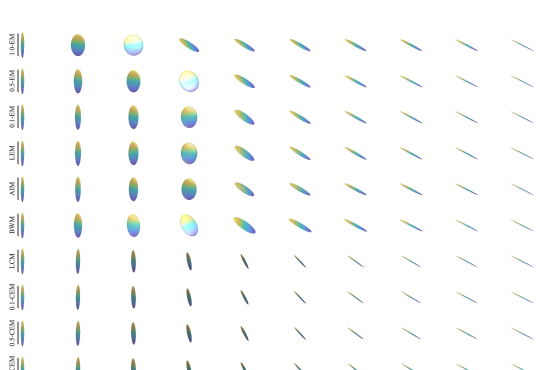
Figure 1: Geodesic interpolation of SPD matrices under different Riemannian metrics. There are four groups of visually different interpolations: (1) $\theta\text{-EM}$; (2) LEM and AIM; (3) BWM; (4) LCM and $\theta\text{-CDEM}$.

7.1 Numerical stability

As discussed at the end of Sec. 5, the core calculation of our metrics relies on diagonal power, while the existing CM uses diagonal exponentiation and logarithm. Therefore, it is expected that our metrics offer better numerical stability and robustness than the existing one. Take the geodesic on the Cholesky manifold as an example. We randomly generate synthetic $n\times n$ Cholesky matrices $L$ and tangent vector $X\in\mathcal{L}^{n}$, with each element’s absolute value uniformly distributed in the interval $[0,1]$. We manually change the smallest eigenvalue (diagonal element) of $L$ into the order of EPS to test the stability. We focus on two dimensionalities: $3\times 3$ for the small matrix and $256\times 256$ for the large matrix. The former one is widely used in diffusion tensor imaging [3], while the latter one is used in computer vision [28, 48]. We set the power deformation $\theta$ as 0.5 and 1.5, respectively. We repeat this process over $100,000$ pairs of $L$ and $X$. The results are shown in Tab. 4. On the dimension of $3\times 3$, the geodesic under the existing CM starts to deteriorate at EPS=$1e^{-3}$, while the ones under our $\theta\text{-DEM}$ and $(\theta,\mathbb{M})\text{-DBWM}$ are stable even down to a high precision $1e^{-15}$, and beyond. As the dimensionality increases to 256, deterioration in the CM geodesic becomes more likely. The geodesic under CM starts to deteriorate at EPS=$1e^{-1}$. In contrast, our metrics show consistent stability. The above comparison demonstrates the numerical advantage of our metrics over the existing CM.

Table 4: Failure probabilities (%) of geodesics under different metrics with small eigenvalues in $L$ on the order of EPS. An output matrix containing any Inf or NaN is considered a failure case. The experiments are conducted on two dimensionalities: $3\times 3$ for small matrices and $256\times 256$ for large matrices.

(a) $3\times 3$ for small matrices.

EPS	CM	$\theta=0.5$		$\theta=1.5$
		$\theta\text{-DEM}$	$(\theta,\mathbb{M})\text{-DBWM}$	$\theta\text{-DEM}$	$(\theta,\mathbb{M})\text{-DBWM}$
$1e^{-1}$	0.62	0	0	0	0
$1e^{-2}$	5.70	0	0	0	0
$1e^{-3}$	51.32	0	0	0	0
$1e^{-4}$	94.34	0	0	0	0
$1e^{-5}$	99.39	0	0	0	0
$1e^{-10}$	100	0	0	0	0
$1e^{-15}$	100	0	0	0	0

(b) $256\times 256$ for large matrices.

EPS	CM	$\theta=0.5$		$\theta=1.5$
		$\theta\text{-DEM}$	$(\theta,\mathbb{M})\text{-DBWM}$	$\theta\text{-DEM}$	$(\theta,\mathbb{M})\text{-DBWM}$
$1e^{-1}$	14.05	0	0	0	0
$1e^{-2}$	18.18	0	0	0	0
$1e^{-3}$	57.86	0	0	0	0
$1e^{-4}$	95.14	0	0	0	0
$1e^{-5}$	99.53	0	0	0	0
$1e^{-10}$	100	0	0	0	0
$1e^{-15}$	100	0	0	0	0

7.2 Tensor interpolation

As shown in [2, 3], proper interpolation of SPD matrices is important in diffusion tensor imaging. The straightforward extension of linear interpolation on Riemannian manifolds is the geodesic interpolation, i.e., the interpolation by a geodesic. This subsection illustrates the geodesic interpolation under different metrics on SPD manifolds.

As shown in Sec. C.1, the geodesics under $\theta\text{-CDEM}$ and $(\theta,\mathbb{M})\text{-CDBWM}$ have a similar expression. Therefore, we focus on $\theta\text{-CDEM}$. Fig. 1 visualizes the geodesic interpolations on $\mathcal{S}^{3}_{++}$ under different metrics, including $\theta\text{-EM}$, LEM, AIM, BWM, LCM, and $\theta\text{-CDEM}$. Tab. 5 presents the associated determinant of each interpolated SPD matrix. We can make the following observation. Firstly, the standard EM exhibits a significant swelling effect, where the maximal determinant of interpretation is extremely larger than the determinants of the starting and end points. Although matrix power $\operatorname{Pow}_{\theta}$ can mitigate the swelling effect ($\theta\text{-EM}\rightarrow\text{LEM}$ with $\theta\rightarrow 0$ [42]), $\theta\text{-EM}$ still suffers from this effect. Additionally, we find that BWM also demonstrates a clear swelling effect. In contrast, LCM, AIM, and LEM show no swelling effect. Besides, the standard CDEM considerably mitigates the swelling effect compared to the standard EM, but it still exhibits some level of swelling. However, by introducing Cholesky power deformation, $\theta\text{-CDEM}$ effectively reduces the swelling effect. Notably, the swelling effect of $\theta\text{-CDEM}$ is significantly weaker than that of $\theta\text{-EM}$ under the same $\theta$. Lastly, the interpolations are different, leaving four kinds of visually different interpolations: (1) $\theta\text{-EM}$; (2) LEM and AIM; (3) BWM; (4) LCM and $\theta\text{-CDEM}$. Notably, compared with other metrics, we observe that the interpolations of LCM and $\theta\text{-CDEM}$ are more visually smoother.

Table 5: The determinants of geodesic interpolations on the SPD manifold. Rows are highlighted in varying shades of green: deeper greens indicate clearer swelling effects.

Metric	The determinant of the $i$-th interpolation
	0	1	2	3	4	5	6	7	8	9
1.0-EM	3.07	104.86	182.09	234.38	261.35	262.64	237.86	186.64	108.61	3.38
0.5-EM	3.07	18.67	39.93	59.53	71.96	73.79	64.14	45.01	21.73	3.38
0.1-EM	3.07	4.25	5.42	6.38	6.96	7.05	6.62	5.75	4.6	3.38
LEM	3.07	3.1	3.14	3.17	3.2	3.24	3.27	3.31	3.34	3.38
AIM	3.07	3.1	3.14	3.17	3.2	3.24	3.27	3.31	3.34	3.38
BWM	3.07	15.32	32.04	48.14	59.22	62.09	55.33	39.93	19.98	3.38
LCM	3.07	3.1	3.14	3.17	3.2	3.24	3.27	3.31	3.34	3.38
0.1-CDEM	3.07	3.15	3.23	3.29	3.34	3.37	3.39	3.4	3.4	3.38
0.5-CDEM	3.07	3.35	3.59	3.79	3.91	3.97	3.94	3.83	3.64	3.38
1.0-CDEM	3.07	3.6	4.07	4.46	4.72	4.83	4.76	4.49	4.03	3.38

7.3 Applications into SPD neural networks

Recently, deep learning on the SPD manifold has shown promising performance in different applications [23, 6, 8, 26, 25, 49]. To further verify the effectiveness of the proposed $\theta\text{-CDEM}$ and $(\theta,\mathbb{M})\text{-CDBWM}$, we apply our metrics to SPD neural networks. We focus on the classic SPDNet backbone [24], mimicking the feedforward neural networks. SPDNet uses the matrix logarithm to map SPD features into the tangent space for classification, which might distort the innate geometry. Recently, [37, 10, 12] generalized the Euclidean Multinomial Logistic Regression (MLR), i.e., Fully Connected (FC) layer + Softmax, into SPD manifolds for intrinsic classification. Following [12], the SPD MLRs under $\theta\text{-CDEM}$ and $(\theta,\mathbb{M})\text{-CDBWM}$ can be obtained, which are presented in Sec. C.2.1.

Table 6: Results of SPDNet with different classifiers on the Radar and HDM05 datasets. The best two results are highlighted in red and blue. The right-most table reports the average training time (s/epoch) of SPDNet with different classifiers under the architecture of 2- and 3-block on the Radar and HDM05 datasets, respectively.

(a) Results on the Radar dataset.
Architecture	2-Block
SPDNet	92.88±1.05
SPDNet-LCM	93.49±1.25
SPDNet-1-CDEM	95.24±0.55
SPDNet-1-CDBWM	93.35±1.02
SPDNet-0.5-CDBWM	93.93±0.79

(b) Results on the HDM05 dataset.
Architecture	2-Block	3-Block
SPDNet	60.69±0.66	60.76±0.80
SPDNet-LCM	62.61±1.46	62.33±2.15
SPDNet-1-CDEM	63.04±1.38,	65.48±2.01
SPDNet-1.5-CDEM	65.48±1.97	66.88±1.66
SPDNet-1-CDBWM	61.28±1.55	64.36±1.74
SPDNet-1.5-CDBWM	62.39±1.77	64.90±1.39

(c) Training efficiency (s/epoch).
Dataset	Radar	HDM05
SPDNet	0.91	2.05
SPDNet-LCM	0.87	3.1
SPDNet-1.5-CDBWM	0.87	3.22
SPDNet-1.5-CDEM	0.87	3.27

We compared our $\theta\text{-CDEM}$ and $(\theta,\mathbb{M})\text{-CDBWM}$ against LCM regarding SPD MLR. The SPD MLR under LCM can be found in [10, Cor. 4.1]. We replace the non-intrinsic classifier (matrix logarithm + FC + Softmax) with the SPD MLR based on LCM, $\theta\text{-CDEM}$ or $(\theta,\mathbb{M})\text{-CDBWM}$. For simplicity, we set $\mathbb{M}$ as the identity matrix. Following [6, 12], we adopt Radar [6] and HDM05 [33] datasets. Following [23, 6], we adopt a 2-block architecture on the Radar dataset, and 2-block and 3-block on the HDM05 dataset. For the deformation parameter $\theta$, we roughly select its value around its deformation boundary, i.e., {0.5,1,1.5}. For $\theta\text{-CDEM}$ or $(\theta,\mathbb{M})\text{-CDBWM}$, if the SPD MLR under the standard metric is already saturated, we will only report the standard one. For more experimental details, please refer to Sec. C.2.

The 10-fold average results are presented in Tab. 6, where SPDNet-[Metric_Name] denotes the SPDNet with an SPD MLR under a certain metric. On both datasets, the SPD MLRs induced by LCM, $\theta\text{-CDEM}$, and $(\theta,\mathbb{M})\text{-CDBWM}$ can further improve the performance of SPDNet, showing superior performance against the vanilla non-intrinsic tangent classifier. Moreover, the SPD MLRs induced by $\theta\text{-CDEM}$ and $(\theta,\mathbb{M})\text{-CDBWM}$ surpass the one induced by LCM. This advantage might come from the following fact. The diagonal logarithm and exponentiation in LCM might overly stretch the diagonal elements, which are the eigenvalues of the Cholesky matrices. In contrast, the diagonal power in our metrics is much more moderate, contributing to a more advantageous performance. Besides, the deformation factor $\theta$ can further improve the associated SPD MLRs, demonstrating the effectiveness of our diagonal deformation. The training efficiency reported in Tab. 6 indicates that our metric enjoys comparable efficiency with LCM.

8 Conclusion

In this paper, we identify the product structures in the Cholesky manifold and propose two new Riemannian metrics on the Cholesky manifold. Two new metrics on the SPD manifolds are induced via Cholesky decomposition, termed as $\theta\text{-CDEM}$ and $(\theta,\mathbb{M})\text{-CDBWM}$. We also discuss the induced gyrovector spaces. Similar to the existing LCM, our metrics have efficient and closed forms for Riemannian operators, including geodesics, Riemannian logarithm, weighted Fréchet mean, and parallel transport along the geodesic. Besides, our metrics have better numeric stability than the existing LCM. Experiments on numerical stability, tensor interpolation, and SPD neural networks demonstrate the effectiveness of our metrics in different applications. We expect that our metrics can offer effective alternatives to existing metrics.

Future Work: Notably, the product structure of the Cholesky manifold unveiled by our work offers new insights into designing Riemannian metrics on the SPD manifold. Def. 3.2 indicates that every Riemannian metric on $\mathbb{R}_{++}$ can induce a metric on the Cholesky manifold and, therefore, on the SPD manifold by the pullback of the Cholesky decomposition. As a future avenue, we will further explore these product geometries to design more effective Riemannian metrics on the SPD manifold. Besides, the gyro structures and closed-form Riemannian operators induced by our metrics offer various possibilities for applying SPD geometries to different applications. As another future avenue, we plan to apply our metrics to other real-world applications.

Appendix A Preliminaries

A.1 Gyrovector spaces

We first recap gyrogroups and gyrocommutative gyrogroups [47], and proceed with gyrovector spaces [36].

Definition A.1 (Gyrogroups [47]).

Given a nonempty set $G$ with a binary operation $\oplus:G\times G\rightarrow G$, $\{G,\oplus\}$ forms a gyrogroup if its binary operation satisfies the following axioms for any $a,b,c\in G$ :

(G1) There is at least one element $e\in G$ called a left identity such that $e\oplus a=a$.

(G2) There is an element $\ominus a\in G$ called a left inverse of $a$ such that $\ominus a\oplus a=e$.

(G3) There is an automorphism $\operatorname{gyr}[a,b]:G\rightarrow G$ for each $a,b\in G$ such that

(89) $$a\oplus(b\oplus c)=(a\oplus b)\oplus\operatorname{gyr}[a,b]c\quad\text{ (Left Gyroassociative Law). }$$

The automorphism $\operatorname{gyr}[a,b]$ is called the gyroautomorphism, or the gyration of $G$ generated by $a,b$. (G4) $\operatorname{gyr}[a,b]=\operatorname{gyr}[a\oplus b,b]$ (Left Reduction Property).

Definition A.2 (Gyrocommutative Gyrogroups [47]).

A gyrogroup $\{G,\oplus\}$ is gyrocommutative if it satisfies

(90) $$a\oplus b=\operatorname{gyr}[a,b](b\oplus a)\quad\text{ (Gyrocommutative Law). }$$

Definition A.3 (Gyrovector Spaces [35]).

A gyrocommutative gyrogroup $\{G,\oplus\}$ equipped with a scalar multiplication $\odot:\mathbb{R}\times G\rightarrow G$ is called a gyrovector space if it satisfies the following axioms for $s,t\in\mathbb{R}$ and $a,b,c\in G$:

(V1) $1\odot a=a,0\odot a=t\odot e=e,\text{ and }(-1)\odot a=\ominus a$.

(V2) $(s+t)\odot a=s\odot a\oplus t\odot a$.

(V3) $(st)\odot a=s\odot(t\odot a)$.

(V4) $\operatorname{gyr}[a,b](t\odot c)=t\odot\operatorname{gyr}[a,b]c$.

(V5) $\operatorname{gyr}[s\odot a,t\odot a]=\mathrm{Id}$, where Id is the identity map.

Note that the gyrovector space defined in [35] is slightly different from the one in [47]. In this paper, we focus on the one in [35].

A.2 Riemannian isometries

This subsection reviews some basic properties of Riemannian isometries. For a more in-depth discussion, please refer to [14, 16].

Let $\{\mathcal{M},g\}$ and $\{\mathcal{N},\tilde{g}\}$ be two Riemannian manifolds, and $\phi:\mathcal{M}\rightarrow\mathcal{N}$ be a Riemannian isometry, i.e., $g=\phi^{*}\tilde{g}$. We denote $\operatorname{Log}$, $\operatorname{Exp}$, $\gamma$, $\mathrm{PT}$, $\operatorname{d}(\cdot,\cdot)$, and $\operatorname{WFM}$ are the Riemannian logarithm, exponentiation, geodesic, parallel transportation along the geodesic, geodesic distance, and weighted Fréchet mean on $\{\mathcal{M},g\}$, while $\widetilde{\operatorname{Log}}$, $\widetilde{\operatorname{Exp}}$, $\widetilde{\gamma}$, $\widetilde{\mathrm{PT}}$, $\widetilde{\operatorname{d}}(\cdot,\cdot)$, and $\widetilde{\operatorname{WFM}}$ are the counterparts on $\{\mathcal{N},\tilde{g}\}$. For $P,Q\in\mathcal{M}$, $V,W\in T_{P}\mathcal{M}$, and $\{P_{i}\in\mathcal{M}\}_{i=1}^{N}$ with weights $\{w_{i}\}_{i=1}^{N}$ satisfying $w_{i}>0$ for all $i$ and $\sum_{i=1}^{N}w_{i}=1$, we have the following:

(91) $$\gamma_{(P,V)}(t) =\phi^{-1}\left(\tilde{\gamma}_{(\phi(P),\phi_{*,P}(V))}(t)\right),$$

(92) $$\operatorname{Log}_{P}(Q) =(\phi_{*,P})^{-1}\left(\widetilde{\operatorname{Log}}_{\phi(P)}\left(\phi(Q)\right)\right),$$

(93) $$\operatorname{Exp}_{P}(V) =\phi^{-1}\left(\widetilde{\operatorname{Exp}}_{\phi(P)}\left(\phi_{*,P}(V)\right)\right),$$

(94) $$\operatorname{PT}_{P\rightarrow Q}(V) =(\phi_{*,Q})^{-1}\left(\widetilde{\mathrm{PT}}_{\phi(P)\rightarrow\phi(Q)}\left(\phi_{*,P}(V)\right)\right),$$

(95) $$\operatorname{d}(P,Q) =\widetilde{\operatorname{d}}(\phi(P),\phi(Q)),$$

(96) $$\operatorname{WFM}(\{P_{i}\},\{w_{i}\}) =\phi^{-1}\left(\widetilde{\operatorname{WFM}}\left(\{\phi(P_{i})\},\{w_{i}\}\right)\right),$$

where $\gamma_{(P,V)}(t)$ is the geodesic starting at $P$ with initial velocity $V\in T_{P}\mathcal{M}$, and $\phi_{*,P}:T_{P}\mathcal{M}\rightarrow T_{\phi(P)}\mathcal{N}$ is the differential map of $\phi$ at $P$. Eq. 96 is the direct corollary of Eq. 95.

Appendix B Riemannian and gyro operators under $(\theta,\mathbb{M})\text{-DBWM}$

B.1 Riemannian operators under $(\theta,\mathbb{M})\text{-DBWM}$

We first define a map $\phi_{\theta}:\mathcal{L}_{++}^{n}\rightarrow\mathcal{L}_{++}^{n}$ as

(97) $$\phi_{\theta}(L)=\lfloor L\rfloor+\mathbb{L}^{\theta},\forall L\in\mathcal{L}_{++}^{n}.$$

Its differential at $L\in\mathcal{L}_{++}^{n}$ is given as

(98) $$\phi_{\theta*,L}(X)=\lfloor X\rfloor+\theta\mathbb{L}^{\theta-1}\mathbb{X},\forall X\in T_{L}\mathcal{L}_{++}^{n}.$$

Let $g^{\mathbb{M}\text{-DBW}}$ and $g^{(\theta,\mathbb{M})\text{-DBW}}$ be $\mathbb{M}\text{-DBWM}$ and $(\theta,\mathbb{M})\text{-DBWM}$, respectively. Since constant scaling of a Riemannian metric preserves the Christoffel symbols, the Riemannian operators such as Riemannian logarithm, exponentiation, and parallel transportation under $g^{(\theta,\mathbb{M})\text{-DBW}}$ is the same as the pullback metric $\phi_{\theta}^{*}g^{\mathbb{M}\text{-DBW}}$. Following Sec. A.2, these Riemannian operators under $(\theta,\mathbb{M})\text{-DBWM}$ can be obtained by $\phi_{\theta}^{*}g^{\mathbb{M}\text{-DBW}}$. Besides, as constant scaling does not affect WFM, the WFM under $(\theta,\mathbb{M})\text{-DBWM}$ is the same as the one under $\phi_{\theta}^{*}g^{\mathbb{M}\text{-DBW}}$. The latter can be calculated by the properties of isometries presented in Sec. A.2. Therefore, by the properties of isometry in Sec. A.2 and Eqs. 97 and 98, we can obtain all the Riemannian operators.

B.2 Gyro operators under $(\theta,\mathbb{M})\text{-DBWM}$

As the gyro operations are defined by the Riemannian logarithm, exponentiation, and parallel transportation, the gyro operations under $(\theta,\mathbb{M})\text{-DBWM}$ are the same as the one under $\phi_{\theta}^{*}g^{\mathbb{M}\text{-DBW}}$. Besides, according to [37, Lems. 2.21 and 2.22], the Riemannian isometry $\phi_{\theta}$ can pull the gyro structures under $\mathbb{M}\text{-DBWM}$ back to the one under $\phi_{\theta}^{*}g^{\mathbb{M}\text{-DBW}}$. Therefore, we can obtain the gyro operations under $(\theta,\mathbb{M})\text{-DBWM}$ via the ones under $\mathbb{M}\text{-DBWM}$ by the pullback. For simplicity, we denote the gyro operation under $\mathbb{M}\text{-DBWM}$ as $\oplus$ and $\odot$, and the counterparts under $(\theta,\mathbb{M})\text{-DBWM}$ as $\widetilde{\oplus}$ and $\widetilde{\odot}$. Then, the gyro operations for $L,K\in\mathcal{L}_{++}^{n}$ and $t\in\mathbb{R}$ under $(\theta,\mathbb{M})\text{-DBWM}$ are

$$L\widetilde{\oplus}K =\phi_{\theta}^{-1}\left(\phi_{\theta}(L)\oplus\phi_{\theta}(K)\right)$$

(99) $$=\lfloor L\rfloor+\lfloor K\rfloor+\left(\mathbb{L}^{\frac{\theta}{2}}+\mathbb{K}^{\frac{\theta}{2}}-I\right)^{\frac{2}{\theta}},$$

$$t\widetilde{\odot}L =\phi_{\theta}^{-1}\left(t\odot\phi_{\theta}(L)\right)$$

(100) $$=t\lfloor L\rfloor+\left(t\mathbb{L}^{\frac{\theta}{2}}+(1-t)I\right)^{\frac{2}{\theta}}.$$

For the well-definedness of $\widetilde{\oplus}$, $L$ and $K$ should satisfy $\mathbb{L}^{\frac{\theta}{2}}+\mathbb{K}^{\frac{\theta}{2}}-I\in\mathbb{D}_{++}^{n}$, while $\widetilde{\odot}$ requires $t$ and $L$ satisfying $(1-t)I+t\mathbb{L}^{\frac{\theta}{2}}\in\mathbb{D}_{++}^{n}$.

According to [37, Thm. 2.24], $\{\mathcal{L}_{++}^{n},\widetilde{\oplus}\}$ conforms with all the axioms of gyrocommutative gyrogroups, while $\{\mathcal{L}_{++}^{n},\widetilde{\oplus},\widetilde{\odot}\}$ conforms with all the axioms of gyrovector spaces.

Appendix C Experimental details

C.1 Geodesics under $\theta\text{-CDEM}$ and $(\theta,\mathbb{M})\text{-CDBWM}$

Supposing $P=LL^{\top}$ and $Q=KK^{\top}$ as the Cholesky decomposition of $P,Q\in\mathcal{S}^{n}_{++}$, Tab. 2 indicates that the geodesics connecting $P$ and $Q$ under $\theta\text{-CDEM}$ and $(\theta,\mathbb{M})\text{-CDBWM}$ are

(101) $$\theta\text{-CDEM}\text{: } \operatorname{Chol}^{-1}\left[\lfloor L\rfloor+t(\lfloor K\rfloor-\lfloor L\rfloor)+\left(\mathbb{L}^{\theta}+t(\mathbb{K}^{\theta}-\mathbb{L}^{\theta})\right)^{\frac{1}{\theta}}\right],$$

(102) $$(\theta,\mathbb{M})\text{-CDBWM}\text{: } \operatorname{Chol}^{-1}\left[\lfloor L\rfloor+t(\lfloor K\rfloor-\lfloor L\rfloor)+\left(\mathbb{L}^{\frac{\theta}{2}}+t(\mathbb{K}^{\frac{\theta}{2}}-\mathbb{L}^{\frac{\theta}{2}})\right)^{\frac{\theta}{2}}\right].$$

C.2 Details of the experiments on the SPDNet backbone

C.2.1 SPD MLRs

Theorem C.1.

The SPD MLRs under $\theta\text{-CDEM}$ and $(\theta,\mathbb{M})\text{-CDBWM}$ are

(103) $$\theta\text{-CDEM}:p(y=k\mid S\in\mathcal{S}^{n}_{++}) \propto\exp\left[\langle\lfloor K\rfloor-\lfloor L_{j}\rfloor,\lfloor A_{j}\rfloor\rangle+\frac{1}{2\theta}\langle\mathbb{K}^{\theta}-\mathbb{L}_{j}^{\theta},\mathbb{A}_{j}\rangle\right],$$

(104) $$(\theta,\mathbb{M})\text{-CDBWM}:p(y=k\mid S\in\mathcal{S}^{n}_{++}) \propto\exp\left[\langle\lfloor K\rfloor-\lfloor L_{j}\rfloor,\lfloor A_{j}\rfloor\rangle+\frac{1}{4\theta}\langle\mathbb{K}^{\frac{\theta}{2}}-\mathbb{L}_{j}^{\frac{\theta}{2}},\mathbb{M}^{-1}\mathbb{A}_{j}\rangle\right],$$

where $S=KK^{\top}$, and for each class $j=1,\cdots,c$, $P_{j}\in\mathcal{S}^{n}_{++}$, $A_{j}\in\mathcal{L}^{n}$, and $P_{j}=L_{j}L_{j}^{\top}$.

Proof C.2.

Putting the associated operators in Sec. 6.1 into Eq. (19) in [12, Lem. 4.3], one can directly obtain the results.

C.2.2 Datasets and preprocessing

The Radar [6] dataset consists of 3,000 synthetic radar signals. Following the protocol in [6], each signal is split into windows of length 20, resulting in 3,000 SPD covariance matrices of $20\times 20$ equally distributed in 3 classes. The HDM05 [33] dataset contains 2,273 skeleton-based motion capture sequences executed by various actors. Each frame consists of 3D coordinates of 31 joints of the subjects, and each sequence can be, therefore, modeled by a $93\times 93$ covariance matrix. Following the protocol in [6], we trim the dataset down to 2086 sequences scattered throughout 117 classes by removing some under-represented classes.

C.2.3 The SPDNet backbone

SPDNet [24] consists of three basic building blocks

(105) BiMap: $$S^{k}=W^{k}S^{k-1}W^{k},$$

(106) ReEig: $$S^{k}=U^{k-1}\max(\Sigma^{k-1},\epsilon I_{n})U^{k-1\top},$$

(107) LogEig: $$S^{k}=\operatorname{mlog}(S^{k-1}),$$

where $S^{k-1}=U^{k-1}\Sigma^{k-1}U^{k-1\top}$ is the eigendecomposition, and $W^{k}$ is column-wisely orthogonal. BiMap (Bilinear Mapping) and ReEig (Eigenvalue Rectification) are the counterparts of linear and ReLu nonlinear activation functions in Euclidean networks. LogEig layer projects SPD matrices into the tangent space at the identity matrix for classification. However, LogEig might distort the innate geometry of SPD features. Recently, [37, 10, 12] generalized the Euclidean Multinomial Logistic Regression (MLR), i.e., Fully Connected (FC) layer + Softmax, into SPD manifolds for intrinsic classification.

C.2.4 Implementation details

We follow the Pytorch code to implement our experiments. To evaluate the performance of our intrinsic classifiers, we substitute the LogEig MLR (LogEig + FC + Softmax) in SPDNet with the SPD MLRs induced by LCM, $\theta\text{-CDEM}$, and $(\theta,\mathbb{M})\text{-CDBWM}$. On the Radar and HDM05 datasets, the learning rate is $1e^{-2}$, the batch size is 30, and the maximum training epoch is 200, respectively. We use the standard-cross entropy loss as the training objective and optimize the parameters with the Riemannian AMSGrad optimizer [4]. The network architectures are represented as $[d_{0},d_{1},\ldots,d_{L}]$, where the dimension of the parameter in the $i$-th BiMap (Sec. C.2.3) layer is $d_{i}\times d_{i-1}$. Following [23, 6], we adopt the architecture of [20, 16, 8] for a 2-block architecture on the Radar dataset, and [93, 70, 30], and [93, 70, 50, 30] for a 2- and 3-block on the HDM05 dataset. In line with the previous work [23, 6], we use accuracy as the scoring metric for the Radar and HDM05 datasets. Ten-fold experiments on Radar and HDM05 datasets are done with randomized initialization and split.

References

- [1] M. Arnaudon, F. Barbaresco, and L. Yang, Riemannian medians and means with applications to radar signal processing, IEEE Journal of Selected Topics in Signal Processing, 7 (2013), pp. 595–604.
- [2] V. Arsigny, P. Fillard, X. Pennec, and N. Ayache, Fast and simple computations on tensors with log-Euclidean metrics., PhD thesis, INRIA, 2005.
- [3] V. Arsigny, P. Fillard, X. Pennec, and N. Ayache, Geometric means in a novel vector space structure on symmetric positive-definite matrices, SIAM Journal on Matrix Analysis and Applications, 29 (2007), pp. 328–347.
- [4] G. Bécigneul and O.-E. Ganea, Riemannian adaptive optimization methods, arXiv preprint arXiv:1810.00760, (2018).
- [5] R. Bhatia, T. Jain, and Y. Lim, On the Bures-Wasserstein distance between positive definite matrices, Expositiones Mathematicae, 37 (2019), pp. 165–191.
- [6] D. Brooks, O. Schwander, F. Barbaresco, J.-Y. Schneider, and M. Cord, Riemannian batch normalization for SPD neural networks, in Advances in Neural Information Processing Systems, vol. 32, 2019.
- [7] R. Chakraborty, ManifoldNorm: Extending normalizations on Riemannian manifolds, arXiv preprint arXiv:2003.13869, (2020).
- [8] R. Chakraborty, J. Bouza, J. Manton, and B. C. Vemuri, Manifoldnet: A deep neural network for manifold-valued data with applications, IEEE Transactions on Pattern Analysis and Machine Intelligence, (2020).
- [9] R. Chakraborty, C.-H. Yang, X. Zhen, M. Banerjee, D. Archer, D. Vaillancourt, V. Singh, and B. Vemuri, A statistical recurrent model on the manifold of symmetric positive definite matrices, Advances in Neural Information Processing Systems, 31 (2018).
- [10] Z. Chen, Y. Song, G. Liu, R. R. Kompella, X. Wu, and N. Sebe, Riemannian multiclass logistics regression for SPD neural networks, in Proceedings of the IEEE Conference on Computer Vision and Pattern Recognition, 2024.
- [11] Z. Chen, Y. Song, Y. Liu, and N. Sebe, A Lie group approach to Riemannian batch normalization, in The Twelfth International Conference on Learning Representations, 2024.
- [12] Z. Chen, Y. Song, Y. Liu, X. Wu, E. Strano, and N. Sebe, Intrinsic Riemannian classifiers on the deformed SPD manifolds: A unified framework, 2024, https://openreview.net/forum?id=EyWKb7Ltcx.
- [13] Z. Chen, T. Xu, X.-J. Wu, R. Wang, Z. Huang, and J. Kittler, Riemannian local mechanism for SPD neural networks, in Proceedings of the AAAI Conference on Artificial Intelligence, 2023, pp. 7104–7112.
- [14] M. P. Do Carmo and J. Flaherty Francis, Riemannian Geometry, vol. 6, Springer, 1992.
- [15] I. L. Dryden, X. Pennec, and J.-M. Peyrat, Power Euclidean metrics for covariance matrices with application to diffusion tensor imaging, arXiv preprint arXiv:1009.3045, (2010).
- [16] J. Q. Gallier and J. Quaintance, Differential geometry and Lie groups, vol. 12, Springer, 2020.
- [17] O. Ganea, G. Bécigneul, and T. Hofmann, Hyperbolic neural networks, Advances in Neural Information Processing Systems, 31 (2018).
- [18] Z. Gao, C. Xu, F. Li, Y. Jia, M. Harandi, and Y. Wu, Exploring data geometry for continual learning, in Proceedings of the IEEE/CVF Conference on Computer Vision and Pattern Recognition, 2023, pp. 24325–24334.
- [19] I. Grubišić and R. Pietersz, Efficient rank reduction of correlation matrices, Linear Algebra and Its Applications, 422 (2007), pp. 629–653.
- [20] J. Guilleminot and C. Soize, Generalized stochastic approach for constitutive equation in linear elasticity: a random matrix model, International Journal for Numerical Methods in Engineering, 90 (2012), pp. 613–635.
- [21] A. Han, B. Mishra, P. Jawanpuria, and J. Gao, Learning with symmetric positive definite matrices via generalized Bures-Wasserstein geometry, in International Conference on Geometric Science of Information, Springer, 2023, pp. 405–415.
- [22] M. Harandi, M. Salzmann, and R. Hartley, Dimensionality reduction on SPD manifolds: The emergence of geometry-aware methods, IEEE Transactions on Pattern Analysis and Machine Intelligence, 40 (2018), pp. 48–62.
- [23] Z. Huang and L. Van Gool, A Riemannian network for SPD matrix learning, in Thirty-first AAAI Conference on Artificial Intelligence, 2017.
- [24] Z. Huang, C. Wan, T. Probst, and L. Van Gool, Deep learning on Lie groups for skeleton-based action recognition, in Proceedings of the IEEE Conference on Computer Vision and Pattern Recognition, 2017, pp. 6099–6108.
- [25] C. Ju, R. J. Kobler, L. Tang, C. Guan, and M. Kawanabe, Deep geodesic canonical correlation analysis for covariance-based neuroimaging data, in The Twelfth International Conference on Learning Representations, 2024.
- [26] R. Kobler, J.-i. Hirayama, Q. Zhao, and M. Kawanabe, SPD domain-specific batch normalization to crack interpretable unsupervised domain adaptation in EEG, Advances in Neural Information Processing Systems, 35 (2022), pp. 6219–6235.
- [27] M. Lezcano Casado, Trivializations for gradient-based optimization on manifolds, Advances in Neural Information Processing Systems, 32 (2019).
- [28] P. Li, J. Xie, Q. Wang, and Z. Gao, Towards faster training of global covariance pooling networks by iterative matrix square root normalization, in Proceedings of the IEEE conference on computer vision and pattern recognition, 2018, pp. 947–955.
- [29] Z. Lin, Riemannian geometry of symmetric positive definite matrices via Cholesky decomposition, SIAM Journal on Matrix Analysis and Applications, 40 (2019), pp. 1353–1370.
- [30] F. López, B. Pozzetti, S. Trettel, M. Strube, and A. Wienhard, Vector-valued distance and Gyrocalculus on the space of symmetric positive definite matrices, Advances in Neural Information Processing Systems, 34 (2021), pp. 18350–18366.
- [31] L. Malagò, L. Montrucchio, and G. Pistone, Wasserstein Riemannian geometry of gaussian densities, Information Geometry, 1 (2018), pp. 137–179.
- [32] M. Moakher, On the averaging of symmetric positive-definite tensors, Journal of Elasticity, 82 (2006), pp. 273–296.
- [33] M. Müller, T. Röder, M. Clausen, B. Eberhardt, B. Krüger, and A. Weber, Documentation mocap database HDM05, technical report, Universität Bonn, 2007.
- [34] X. S. Nguyen, Geomnet: A neural network based on Riemannian geometries of SPD matrix space and Cholesky space for 3D skeleton-based interaction recognition, in Proceedings of the IEEE International Conference on Computer Vision, 2021, pp. 13379–13389.
- [35] X. S. Nguyen, The Gyro-structure of some matrix manifolds, in Advances in Neural Information Processing Systems, vol. 35, 2022, pp. 26618–26630.
- [36] X. S. Nguyen, A Gyrovector space approach for symmetric positive semi-definite matrix learning, in Proceedings of the European Conference on Computer Vision, 2022, pp. 52–68.
- [37] X. S. Nguyen and S. Yang, Building neural networks on matrix manifolds: A Gyrovector space approach, in International Conference on Machine Learning, PMLR, 2023, pp. 26031–26062.
- [38] X. S. Nguyen, S. Yang, and A. Histace, Matrix manifold neural networks++, in The Twelfth International Conference on Learning Representations, 2024.
- [39] Y.-T. Pan, J.-L. Chou, and C.-S. Wei, Matt: A manifold attention network for EEG decoding, Advances in Neural Information Processing Systems, 35 (2022), pp. 31116–31129.
- [40] X. Pennec, P. Fillard, and N. Ayache, A Riemannian framework for tensor computing, International Journal of Computer Vision, 66 (2006), pp. 41–66.
- [41] O. Skopek, O.-E. Ganea, and G. Bécigneul, Mixed-curvature variational autoencoders, arXiv preprint arXiv:1911.08411, (2019).
- [42] Y. Thanwerdas and X. Pennec, The geometry of mixed-Euclidean metrics on symmetric positive definite matrices, Differential Geometry and its Applications, 81 (2022), p. 101867.
- [43] Y. Thanwerdas and X. Pennec, O (n)-invariant Riemannian metrics on SPD matrices, Linear Algebra and its Applications, 661 (2023), pp. 163–201.
- [44] A. A. Ungar, Analytic hyperbolic geometry: Mathematical foundations and applications, World Scientific, 2005.
- [45] A. A. Ungar, A Gyrovector Space Approach to Hyperbolic Geometry, Springer, 2009.
- [46] A. A. Ungar, Beyond the Einstein addition law and its gyroscopic Thomas precession: The theory of gyrogroups and gyrovector spaces, Springer Science & Business Media, 2012.
- [47] A. A. Ungar, Analytic hyperbolic geometry in n dimensions: An introduction, CRC Press, 2014.
- [48] Q. Wang, J. Xie, W. Zuo, L. Zhang, and P. Li, Deep CNNs meet global covariance pooling: Better representation and generalization, IEEE Transactions on Pattern Analysis and Machine Intelligence, 43 (2020), pp. 2582–2597.
- [49] R. Wang, X.-J. Wu, Z. Chen, C. Hu, and J. Kittler, SPD manifold deep metric learning for image set classification, IEEE Transactions on Neural Networks and Learning Systems, (2024).
- [50] Y. Yuan, H. Zhu, W. Lin, and J. S. Marron, Local polynomial regression for symmetric positive definite matrices, Journal of the Royal Statistical Society Series B: Statistical Methodology, 74 (2012), pp. 697–719.
- [51] W. Zhao, F. Lopez, J. M. Riestenberg, M. Strube, D. Taha, and S. Trettel, Modeling graphs beyond hyperbolic: Graph neural networks in symmetric positive definite matrices, in Joint European Conference on Machine Learning and Knowledge Discovery in Databases, Springer, 2023, pp. 122–139.