Beyond Weak Cramér Rao Bound for Distributed Phases Using Multiphoton Polarization GHZ State: Exact Quantum Fisher Matrix Results

Abstract

Quantum-enhanced parameter estimation is critical in various fields, including distributed sensing. In this study, we focus on estimating multiple unknown phases at different spatial nodes using multiphoton polarization-entangled states. Previous research has relied on a much weaker Cramér-Rao bound rather than precise bounds from exact quantum Fisher information matrices. We present exact results for the distributed sensing. We find that, due to its singular nature, direct use of the quantum Fisher information matrix is not possible. We analyze the reasons for this singularity, which has prevented the determination of quantum Cramér-Rao bounds. We demonstrate that not all phases in distributed sensing with multiphoton entangled states are independent. We obtain non-singular matrices by identifying and removing the redundant phase from the calculation. This allows us to derive exact quantum Cramér-Rao bounds, which we verify are saturated by projective measurements. These bounds enable Heisenberg-limited sensing for the average phase. Our analysis is specifically applicable to N-photon GHZ states distributed across multiple nodes. This advancement is significant as it paves the way for more precise and efficient distributed sensing, enhancing the overall capabilities of quantum sensing technologies based on N photon GHZ states.

I Introduction

In recent decades, quantum metrology has experienced substantial progress [1, 2, 3], especially in distributed quantum sensing [4]. This advanced technique enables the simultaneous examination of systems across multiple spatial locations, which has become a fundamental aspect of quantum networks. These networks consist of interconnected quantum devices that facilitate enhanced distributed computing and secure communication [5]. A significant challenge in this field is achieving precise measurements for multiple parameters due to the Heisenberg uncertainty principle, which imposes fundamental limits on the accuracy of certain pairs of measurements [6, 7, 8]. Entanglement between quantum states at remote nodes is critical for surpassing the measurement capabilities of systems without entanglement [9, 10, 11, 12, 13]. The optimal probe states and measurements for multiple phase estimation are given in [14], which requires special quantum correlations to obtain the minimum total variance. Distributing a single-mode squeezed vacuum state through a balanced beam splitter network allows for precise quadrature displacement estimation, achieving Heisenberg scaling in the number of modes [9, 10]. This state is proven to be the optimal entangled Gaussian state for estimating both displacement and the weighted sum of phase [15]. The scalability of this approach has been illustrated in global random continuous-variable (CV) networks. Kwon et al. showed that most CV quantum networks can achieve Heisenberg scaling for distributed quantum displacement sensing [16]. Additionally, these networks can maintain robustness in the presence of noise by using error correction codes, which help restore Heisenberg scaling even in networks with up to 100 nodes [17].

Complementing these advancements in CV systems, discrete variable (DV) quantum systems have also shown significant promise in quantum sensing. In 2001, Pan et al. [18] achieved a breakthrough by creating a highly pure four-photon Greenberger–Horne–Zeilinger (GHZ) state [19]. The quality of entangled DV states has further increased in recent years [20, 21, 22, 23, 24, 25, 26, 27, 28, 29, 30], showcasing the strong potential of DV systems in quantum sensing. Given their notable scalability and applicability to various quantum technologies, studying the sensing precision of DV systems is essential. Consider a system with $d$ unknown phases $\phi={\phi_{1},\phi_{2},\ldots,\phi_{d}}$ in distinct spatial nodes, where the goal is to estimate a linear combination of these phases. Theoretical demonstrations [31] have shown that Heisenberg scaling is achievable using both mode-entangled and particle-entangled states. This has been experimentally validated for mode numbers $d=3$ [32] and $d=2$ up to 10 km [33]. However, to estimate multiple unknown phases with those states, the number of photons $N$ must be equal to or greater than $d$. Kim et al. [34] introduced the polarization GHZ state for multi-phase estimation, achieving Heisenberg scaling without requiring $N\geq d$. This approach enhanced sensitivity by 2.2 dB for $N=2$ and $d=4$ over 3 km. Kim et al., however, did not use the full quantum metrological framework. They used a much weaker Cramér-Rao bound, which was also used in a previous experimental work [32].

Understanding parameter estimation precision in these quantum systems relies on the quantum Fisher information (QFI) and quantum Cramér-Rao bound (QCRB) [35, 36, 37, 38, 39, 40, 41, 42], which are essential for discerning quantum sensing capabilities [43]. The quantum Fisher information matrix (QFIM) [44, 45, 46, 47, 48, 49, 50, 28] provides insight into parameter correlations and achievable precision. In single-parameter estimation, the QCRB is attainable, and there are well-established methods for identifying the optimal measurement [38, 51]. However, in the multi-parameter scenario, the QCRB for all parameters can not be attained simultaneously unless the optimal measurements for all parameters are compatible [6]. Special conditions are required to determine whether the QCRB can be achieved by certain measurements [52, 14, 53]. Trade-offs arise when dealing with incompatible quantum measurements [54, 55, 56, 57]. In cases with limited parameter dependency understanding, machine learning techniques like Bayesian quantum estimation are employed [58, 59, 60]. Probabilistic protocols with post-selection are proposed to achieve the Heisenberg limit for general network states [61]. However, in [34], using the special multi-partite GHZ states, where complete system information is available, only the weak form of the Cramér-Rao bound (CRB) was analyzed. The same situation is found in [32], where only a combination of phases appears in the system, so it is impossible to determine individual phases. We have examined the applicability of full quantum metrological framework and show that the inability to obtain the exact CRB arises from the singularity of the information matrix (FIM). We show that this singularity occurs because ${\phi_{1},\phi_{2},\ldots,\phi_{d}}$ does not form an independent basis when using the polarization GHZ state for estimation, necessitating proper variable transformation.

Here, we outline the procedure for constructing such variable transformations to construct diagonal or block-diagonal quantum Fisher information matrices. We then obtain the quantum Cramér-Rao bounds for this problem alongside achievable classical CRB derived from probability measurements. It’s noteworthy that the QCRB for the average phase $\bar{\phi}=\sum_{i=1}^{d}\phi_{i}/d$ is $1/N$, which achieves the Heisenberg scaling, for any even number $d$. This procedure allows us to obtain the optimal precision, offering new insights into quantum methods for enhanced sensing of distributed measurements. This paper is structured as follows: In Sec. II, we begin with an illustrative example by focusing on the case where $N=2$ and $d=4$, considering the average phase $\bar{\phi}=\frac{1}{d}(\phi_{1}+\phi_{2}+...+\phi_{d})$ as the parameter to be estimated. In Sec. III, we discuss the singularity of the classical Fisher Information (FI). In Sec. IV, we provide a parameter transformation and derive both the classical Cramér-Rao Bound (CRB) and the Quantum Cramér-Rao Bound (QCRB) for the average phase. In Sec. V, we study the recision - photon number relation by replacing the input photon number $N$ and the number of phases $d$ with any even number, thereby confirming the Heisenberg scaling. Finally, in Sec. VI, we provide a discussion, consolidating the findings and offering insights into the implications of our study.

II Distribution of two-photon entanglement across four nodes and classical Fisher Information

As an example, we consider the scenario where the input photon number $N=2$ and the number of spatially separated phases $d=4$. A polarization GHZ state of two photons, generated via spontaneous parametric down-conversion (SPDC), can be expressed by

$$\ket{\Phi_{a,b}}=\frac{1}{\sqrt{2}}(\ket{H_{a}H_{b}}+\ket{V_{a}V_{b}}),$$ (1)

where $a$ and $b$ denote each photon in the two-photon GHZ state; $H$ and $V$ denote the polarization states of the photons, representing horizontal and vertical orientations, respectively. By adding a beam splitter network that contains two 50:50 beam splitters, the two-photon GHZ state can be split to distribute among four nodes, thus forming the input state of this sensing problem, expressed by

$$\ket{\Phi_{i}}=\frac{1}{2}(\ket{\Phi_{1,2}}+\ket{\Phi_{2,3}}+\ket{\Phi_{3,4}}+\ket{\Phi_{4,1}}).$$ (2)

Here, the different subscripts refer to different spatial nodes. After passing through various phases at different nodes, the input state is transferred to the following output state

$$\ket{\Phi_{o}}= \frac{1}{2\sqrt{2}}(\ket{H_{1}H_{2}}+e^{i(\phi_{1}+\phi_{2})}\ket{V_{1}V_{2}}$$

$$+\ket{H_{2}H_{3}}+e^{i(\phi_{2}+\phi_{3})}\ket{V_{2}V_{3}}$$

$$+\ket{H_{3}H_{4}}+e^{i(\phi_{3}+\phi_{4})}\ket{V_{3}V_{4}}$$

$$+\ket{H_{4}H_{1}}+e^{i(\phi_{4}+\phi_{1})}\ket{V_{4}V_{1}}).$$ (3)

When analyzing such systems, precision becomes crucial. Precision in parameter estimations is quantified by the standard deviation ($\Delta X$) of measured parameter values: $\Delta X=\sqrt{\langle X^{2}\rangle-\langle X\rangle^{2}}$. In systems with multiple parameters, the precision of determining each parameter’s value can be influenced not only by their individual characteristics but also by the covariance between different parameters, which may not be independent. To establish a classical lower bound for this precision, we utilize the classical Fisher information matrix $F_{mn}(X)$. This matrix quantifies the information content about the parameters $X_{m}$ and $X_{n}$ present in the data. Mathematically, it is defined as the expectation value of the second derivative of the log-likelihood function with respect to these parameters:

$$F_{mn}(X)=\langle\frac{\partial^{2}}{\partial X_{m}\partial X_{n}}\ln L(X)\rangle,$$ (4)

where $L(X)$ represents the likelihood function. For discrete data, the likelihood function is the product of the probability mass function (PMF) evaluated at each observed value: $L(X)=\prod_{j}P_{j}(X)$, where $P_{j}(X)$ is the PMF evaluated at the $j$th individual observed value given the parameter values $X$. Thus, it can be written as

$$F_{mn}(X)=\sum_{j}\frac{1}{P_{j}(X)}\frac{dP_{j}(X)}{dX_{m}}\frac{dP_{j}(X)}{dX_{n}}.$$ (5)

The lower bounds (Cramér-Rao bounds) for the variances and covariances are defined as

$$Cov(X_{m},X_{n})\geq F^{-1}_{mn}(X)/{\cal N},$$ (6)

where $F^{-1}_{mn}(X)$ is the Fisher information matrix’s inverse matrix, and ${\cal N}$ is the number of independent measurements.

III Singularity of Classical Fisher Information matrix and the weak Cramér-Rao bound

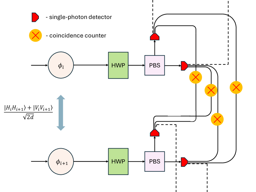
Figure 1: The illustration of the projection measurement method. In this scheme, HWP denotes the half-wave plate, and PBS represents the polarization beam-splitter.

Considering a projective measurement on the $\sigma_{x}$ basis shown in Fig 1, the corresponding probability set comprises sixteen probabilities denoted as ${P_{jk}^{++},P_{jk}^{--},P_{jk}^{+-},P_{jk}^{-+}}$. Here, the superscripts $+$ and $-$ signify the two different basis $\frac{1}{\sqrt{2}}(\ket{H}\pm\ket{V})$, and $jk$ indicates the nodes based on $\phi_{j}$ and $\phi_{k}$, i.e., ${jk}=\{12,23,34,41\}$. For instance, $P_{12}^{+-}$ represents the probability of two-photon coincidence events between observing $+$ in node 1 and $-$ in node 2. The probabilities for the projection measurement are indicated as

$$P_{jk}^{++}=P_{jk}^{--}=\frac{1+\cos(\phi_{j}+\phi_{k})}{16},$$

$$P_{jk}^{+-}=P_{jk}^{-+}=\frac{1-\cos(\phi_{j}+\phi_{k})}{16}.$$ (7)

Kim et al. [34] obtained the classical Fisher information matrix

$$F_{0}=\left(\begin{array}[]{cccc}F_{11}&F_{12}&F_{13}&F_{14}\\ F_{21}&F_{22}&F_{23}&F_{24}\\ F_{31}&F_{32}&F_{33}&F_{34}\\ F_{41}&F_{42}&F_{43}&F_{44}\end{array}\right)=\left(\begin{array}[]{cccc}\frac{1}{2}&\frac{1}{4}&0&\frac{1}{4}\\ \frac{1}{4}&\frac{1}{2}&\frac{1}{4}&0\\ 0&\frac{1}{4}&\frac{1}{2}&\frac{1}{4}\\ \frac{1}{4}&0&\frac{1}{4}&\frac{1}{2}\end{array}\right).$$ (8)

Note that the rank of $F_{0}$ is 3. Thus, an inverse operation can not be applied on $F_{0}$ due to the singularity. They then investigated the precision bound for measuring the average phase $\bar{\phi}=\frac{1}{4}(\phi_{1}+\phi_{2}+\phi_{3}+\phi_{4})$ using the weak form of the Cramér-Rao bound, which for a linear combination of the input $\alpha^{T}\phi=\sum_{i=1}^{d}\alpha_{i}\phi_{i}$ where $\sum_{i=1}^{d}|\alpha_{i}|=1$, is defined as

$$Var(\alpha^{T}\phi)\geq\frac{(\alpha^{T}\alpha)^{2}}{N\alpha^{T}F_{0}\alpha}.$$ (9)

Unlike Eq. (6), this approach does not necessitate the inversion of the FIM. It’s remarkable that they achieved Heisenberg scaling for $\bar{\phi}$ solely relying on the Classical Fisher Information and the weak form of the Cramér-Rao Bound. This underscores the need for a comprehensive quantum analysis of the system’s structure to fully understand and optimize parameter estimation capabilities.

IV QFIM and removal of its singularity-two photon entangled state distributed across four nodes

Expanding this framework to quantum mechanics involves maximizing $F(X)$ over all conceivable quantum measurements, leading to the quantum Fisher information (QFI) ${\cal F}^{(Q)}(X)$. Various techniques exist for obtaining the QFI. Here, given that the final state $\ket{\Phi_{o}}$ is a pure state, the elements in the QFIM can be calculated by

$${\cal F}^{(Q)}_{mn}(X)=4\text{Re}\left(\langle\partial_{X_{m}}\psi\,|\,\partial_{X_{n}}\psi\rangle-\langle\partial_{X_{m}}\psi\,|\,\psi\rangle\,\langle\psi\,|\,\partial_{X_{n}}\psi\rangle\right).$$ (10)

Thus, the corresponding quantum Cramér-Rao bounds are expressed as

$$Cov(X_{m},X_{n})\geq({\cal F}^{(Q)})^{-1}_{mn}(X)/{\cal N}.$$ (11)

Using Eq. (10), we obtain the QFIM of the original set of variables as

$${\cal F}_{0}^{(Q)}=\left(\begin{array}[]{cccc}\frac{3}{4}&\frac{1}{4}&-\frac{1}{4}&\frac{1}{4}\\ \frac{1}{4}&\frac{3}{4}&\frac{1}{4}&-\frac{1}{4}\\ -\frac{1}{4}&\frac{1}{4}&\frac{3}{4}&\frac{1}{4}\\ \frac{1}{4}&-\frac{1}{4}&\frac{1}{4}&\frac{3}{4}\end{array}\right),$$ (12)

The rank of ${\cal F}_{0}^{(Q)}$ is 3, indicating that it is a singular matrix. Consequently, it is not possible to obtain the QCRBs for the four variables, as the inverse operation required by Eq. (11) cannot be performed on a singular QFIM. To deal with the singularity, it is essential to investigate the degree of freedom in this system and identify the independent variables that contribute. we construct an orthogonal transformation as follows: the original variables $\{\phi_{1},\phi_{2},\phi_{3},\phi_{4}\}$ can be orthogonally transformed to new basis $\{\phi_{0},\phi_{a},\phi_{b},\phi_{c}\}$, where

$$\phi_{0}=\frac{\phi_{1}-\phi_{2}+\phi_{3}-\phi_{4}}{2},\,\,\,\,\phi_{a}=\frac{\phi_{1}+\phi_{2}+\phi_{3}+\phi_{4}}{2},$$

$$\phi_{b}=\frac{\phi_{1}+\phi_{2}-\phi_{3}-\phi_{4}}{2},\,\,\,\,\phi_{c}=\frac{\phi_{1}-\phi_{2}-\phi_{3}+\phi_{4}}{2}.$$ (13)

The output state can thus be expressed as

$$\ket{\Phi_{o}}= \frac{1}{2\sqrt{2}}(\ket{H_{1}H_{2}}+e^{i(\phi_{a}+\phi_{b})}\ket{V_{1}V_{2}}$$

$$+\ket{H_{2}H_{3}}+e^{i(\phi_{a}-\phi_{c})}\ket{V_{2}V_{3}}$$

$$+\ket{H_{3}H_{4}}+e^{i(\phi_{a}-\phi_{b})}\ket{V_{3}V_{4}}$$

$$+\ket{H_{4}H_{1}}+e^{i(\phi_{a}+\phi_{c})}\ket{V_{4}V_{1}}).$$ (14)

Note that $\ket{\Phi_{o}}$ depends only on three variables, $\phi_{a}$, $\phi_{b}$, and $\phi_{c}$, while $\phi_{0}$ does not contribute.

Using Eq. (10), the QFIM of the set of variables $\{\phi_{a},\,\phi_{b},\,\phi_{c}\}$ is obtained as

$${\cal F}^{(Q)}=\left(\begin{array}[]{ccc}{\cal F}^{(Q)}_{aa}&{\cal F}^{(Q)}_{ab}&{\cal F}^{(Q)}_{ac}\\ {\cal F}^{(Q)}_{ba}&{\cal F}^{(Q)}_{bb}&{\cal F}^{(Q)}_{bc}\\ {\cal F}^{(Q)}_{ca}&{\cal F}^{(Q)}_{cb}&{\cal F}^{(Q)}_{cc}\end{array}\right),$$ (15)

where

$${\cal F}_{aa}^{(Q)} =\frac{7}{4}-\frac{1}{8}(\cos 2\phi_{b}+\cos 2\phi_{c}+4\cos\phi_{b}\cos\phi_{c}),$$

$${\cal F}_{ab}^{(Q)} =({\cal F}_{ba}^{(Q)})^{*}=-\frac{i}{4}\cos\phi_{b}\sin\phi_{c}-\frac{i}{8}\sin 2\phi_{b},$$

$${\cal F}_{ac}^{(Q)} =({\cal F}_{ca}^{(Q)})^{*}=-\frac{i}{4}\sin\phi_{b}\cos\phi_{c}-\frac{i}{8}\sin 2\phi_{c},$$

$${\cal F}_{bb}^{(Q)} =\frac{7}{8}+\frac{1}{8}\cos 2\phi_{b},$$

$${\cal F}_{cc}^{(Q)} =\frac{7}{8}+\frac{1}{8}\cos 2\phi_{c},$$

$${\cal F}_{bc}^{(Q)} ={\cal F}_{cb}^{(Q)}=-\frac{1}{4}\sin\phi_{b}\sin\phi_{c}.$$

Considering weak phase shifts that $\phi_{a,b,c}\ll 1$, ${\cal F}^{(Q)}$ becomes the 3-dimensional identity matrix $I_{3}$. Thus, the quantum Cramér-Rao bound for $\bar{\phi}$ is

$$\Delta_{q}\bar{\phi}=\frac{1}{2}\Delta_{q}\phi_{a}\geq\frac{1}{2},$$ (16)

which achieves the Heisenberg scaling $\Delta\bar{\phi}\geq 1/N$ with a two-photon input. Note that Eq.(15) remains valid for any combination where $\phi_{b}=\phi_{c}=0$, i.e., as long as $\phi_{1}=\phi_{3}$ and $\phi_{2}=\phi_{4}$, the Quantum Cramer-Rao Bounds (QCRBs) for $\phi_{a},\phi_{b},$ and $\phi_{c}$ achieve the Heisenberg scaling. Additionally, for cases where $\phi_{c}=\pm\phi_{b}=n\pi$ for any integer $n$, Eq.(15) still holds. In the following, we focus primarily on weak phase sensing where $\phi_{a,b,c}\ll 1$.

Considering the same measurement scheme as in Eq. (III), yet after constructing the transformation in Eq. (IV), we can write Eq. (III) with the new set of variables. Considering weak phase shifts that $\phi_{a,b,c}\ll 1$, the classical Fisher information matrix is obtained as

$$F=\left(\begin{array}[]{ccc}F_{aa}&F_{ab}&F_{ac}\\ F_{ba}&F_{bb}&F_{bc}\\ F_{ca}&F_{cb}&F_{cc}\end{array}\right)=\left(\begin{array}[]{ccc}1&0&0\\ 0&\frac{1}{2}&0\\ 0&0&\frac{1}{2}\end{array}\right),$$ (17)

which is a $3\times 3$ full-rank diagonal matrix. Thus, the classical Cramér-Rao bound $\Delta_{c}\bar{\phi}$ for $\bar{\phi}=\frac{1}{2}\phi_{a}$ is

$$\Delta_{c}\bar{\phi}=\frac{1}{2}\Delta_{c}\phi_{a}\geq\frac{1}{2}.$$ (18)

It reaches the Heisenberg scaling $\Delta\bar{\phi}\geq\frac{1}{N}$ with a two-photon input. Furthermore, it demonstrates that the weak bound obtained in reference [34] attains the exact Cramér-Rao bound for the average phase in this scenario. It’s noteworthy that the result specifically pertains to the average $\bar{\phi}$ here, where both the classical and quantum bounds coincide. This suggests that the projection measurement in [34] serves as an optimal measurement scheme for estimating $\bar{\phi}$. However, the quantum Cramér-Rao bound is below the counterpart when our interest extends beyond $\bar{\phi}$ to encompass parameters such as $\phi_{b}$, $\phi_{c}$, or other linear combinations within ${\phi_{1},\phi_{2},\phi_{3},\phi_{4}}$, as shown in Eq. (17). Other measurement schemes should be considered in that case.

V N-photon entangled states on a network with d nodes

V.1 Symmetry of the system

To further study the relationship between precision and photon number in this system, we consider the most general case containing d independent phases $\{\phi_{1},\ldots,\phi_{d}\}$ located at various spatial positions. Using a beam splitter network equipped with an increased number of beam splitters allows for the investigation of such distributed systems with a greater number of spatial nodes. Upon distribution, as shown in Fig. 2, the N-photon polarization Bell state is expressed by

$$\ket{\Psi_{d}^{N}}_{i}=\frac{1}{\sqrt{2d}}\sum_{j=1}^{d}(\ket{H_{j}}^{\otimes\frac{N}{2}}\ket{H_{j+1}}^{\otimes\frac{N}{2}}+\ket{V_{j}}^{\otimes\frac{N}{2}}\ket{V_{j+1}}^{\otimes\frac{N}{2}}),$$ (19)

where notations $\ket{H_{d+1}}:=\ket{H_{1}}$ and $\ket{V_{d+1}}:=\ket{V_{1}}$. This system exhibits symmetry on the indexes $\{1,2,\ldots,d\}$ under certain cyclic permutations. Let us consider a cyclic permutation denoted by $\sigma$, which reorders elements in a sequence by shifting each element to the position of its successor, with the final element returning to the initial position. Mathematically, this operation is represented by $\sigma(j)=j+1$ for $j\neq d$, and $\sigma(d)=1$. This process preserves the sequential order of elements in a cyclical manner. Notably, Eq. (19) remains unchanged under the action of $\sigma$ and its integral powers.

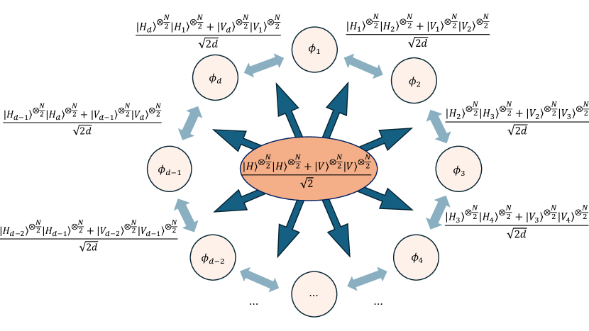
Figure 2: State distribution for measurement of phases located in distinct spatial nodes.

As the photons propagate through the phases situated at the $d$ nodes, the resulting output state becomes

$$\ket{\Psi_{d}^{N}}_{o} =\frac{1}{\sqrt{2d}}\sum_{j=1}^{d}(\ket{H_{j}}^{\otimes\frac{N}{2}}\ket{H_{j+1}}^{\otimes\frac{N}{2}}$$

$$+e^{i\frac{N}{2}(\phi_{j}+\phi_{j+1})}\ket{V_{j}}^{\otimes\frac{N}{2}}\ket{V_{j+1}}^{\otimes\frac{N}{2}}),$$ (20)

where $\phi_{d+1}:=\phi_{1}$. Note that the evolution of this system does not break its symmetry.

V.2 The singularity of the QFIM

Using Eq. (10), we obtain the QFIM ${\cal F}_{0}^{(Q)}$ of the original set of variables, which elements are:

$${\cal F}_{jj}^{(Q)} =\frac{N^{2}}{d^{2}}(d-1),$$

$${\cal F}_{jj+1}^{(Q)} =\frac{N^{2}}{d^{2}}(\frac{d}{2}-1),$$

$${\cal F}_{jj+k}^{(Q)} =-\frac{N^{2}}{d^{2}},\qquad(k\geq 2).$$ (21)

The determinant of ${\cal F}_{0}^{(Q)}$ can be calculated using the Leibniz formula

$$\det({\cal F}_{0}^{(Q)})=\sum_{\sigma\in S_{n}}\text{sgn}(\sigma)\prod_{j=1}^{n}({\cal F}_{0}^{(Q)})_{j,\sigma(j)}.$$ (22)

Consider any row of ${\cal F}_{0}^{(Q)}$, which contains ${\cal F}_{j1}^{(Q)}$, ${\cal F}_{j2}^{(Q)}$, $\ldots$, ${\cal F}_{jd}^{(Q)}$. The combination $\sum_{k=1}^{d}(-1)^{k}({\cal F}_{0}^{(Q)})_{jk}=0$, indicating that the columns of ${\cal F}_{0}^{(Q)}$ form a linearly dependent set. Consequently, the determinant of ${\cal F}_{0}^{(Q)}$ is $0$, implying that ${\cal F}_{0}^{(Q)}$ is singular.

V.3 Finding the irrelevant variable

To examine the system’s degree of freedom, we consider a linear combination of the variables defined as $\theta_{0}:=\frac{1}{d}\sum_{j=1}^{d}(-1)^{j}\phi_{j}:=\overrightarrow{c_{0}}\cdot\overrightarrow{\phi}$. We demonstrate the independence of the system’s evolution on $\theta_{0}$ by considering the following variable transformation:

$$(\theta_{0},\theta_{1},\theta_{2},\cdots,\theta_{d-1})^{T}=M_{c}\cdot(\phi_{1},\phi_{2},\phi_{3},\cdots,\phi_{d})^{T},$$ (23)

where $\theta_{1}=\overrightarrow{c_{1}}\cdot\overrightarrow{\phi}=\bar{\phi}$ being the average phase. Thus $\overrightarrow{c_{1}}=(\frac{1}{d},\cdots,\frac{1}{d})$. It’s apparent that $\overrightarrow{c_{1}}\bot\overrightarrow{c_{0}}$. We then let $\theta_{i}=\overrightarrow{c_{i}}\cdot\overrightarrow{\phi}=\frac{1}{d}(\phi_{i-1}-\phi_{i+1})$ for $2\leq i\leq(d-1)$. Note that $\overrightarrow{c_{i}}\bot\overrightarrow{c_{0}}$ and $\overrightarrow{c_{i}}\bot\overrightarrow{c_{1}}$ for $2\leq i\leq(d-1)$. The transformation described can be defined by the transformation matrix

$$M_{c}=\left(\begin{array}[]{c}\overrightarrow{c_{0}}\\ \overrightarrow{c_{1}}\\ \overrightarrow{c_{2}}\\ \overrightarrow{c_{3}}\\ \vdots\\ \overrightarrow{c_{d-2}}\\ \overrightarrow{c_{d-1}}\end{array}\right)=\frac{1}{d}\left(\begin{array}[]{ccccccc}-1&1&-1&1&-1&\cdots&1\\ 1&1&1&1&1&\cdots&1\\ 1&0&-1&0&0&\cdots&0\\ 0&1&0&-1&0&\cdots&0\\ \vdots&\vdots&\vdots&\vdots&\vdots&\ddots&\vdots\\ 0&\cdots&0&1&0&-1&0\\ 0&\cdots&0&0&1&0&-1\end{array}\right),$$ (24)

where for $1\leq i\leq d$,

$$(M_{c})_{1i} =\frac{1}{d}(-1)^{i},\qquad(M_{c})_{2i}=\frac{1}{d},$$

$$(M_{c})_{ji} =\frac{1}{d}[\delta(j-2,i)-\delta(j,i),\quad\text{for}\quad(3\leq j\leq d)].$$

Here the notation $\delta(x_{1},x_{2})$ refers to the kronecker delta, defined as $\delta(x_{1},x_{2})=1$ if $x_{1}=x_{2}$, and $\delta(x_{1},x_{2})=0$ otherwise. It’s important to note that this transformation is not orthogonal. Specifically, not every pair of variables $\varphi_{i}$ and $\varphi_{j}$ within this set are orthogonal; for example, $\overrightarrow{c_{i}}\cdot\overrightarrow{c_{i+1}}=1/d^{2}$ for $2\leq i\leq(d-2)$. However, as long as this transformation is invertible, orthogonality is not a prerequisite, as our primary concern is for the quantum Fisher information matrix (QFIM) to be block diagonal. In the case of the transformation described in Equation (24), the elements of the inverse transformation matrix $M_{c}^{-1}$ are

$$(M_{c}^{-1})_{i1} =(-1)^{i},\qquad(M_{c}^{-1})_{i2}=1,$$

$$(M_{c}^{-1})_{ij} =d\delta[(-1)^{i},(-1)^{j}]\{H(j-i)(1-\frac{j-2+\delta[(-1)^{i},1]}{d})$$

$$-H(i-j)\frac{j-2+\delta[(-1)^{i},1]}{d}\},\;\;\;\;\text{for}\;\;\;(3\leq j\leq d).$$ (25)

In this context, $H(x)$ represents a modified Heaviside function, defined as $H(x)=1$ if $x\geq 0$, and $H(x)=0$ otherwise.

We analyze the dependence of the system on the variable $\theta_{0}$

$$\partial_{\theta_{0}} \ket{\Psi_{d}^{N}}_{o}=\sum_{i=1}^{d}\frac{\partial{\phi_{i}}}{\partial{\theta_{0}}}\partial_{\phi_{i}}\ket{\Psi_{d}^{N}}_{o}$$

$$=i\frac{N}{2d}\sum_{i=1}^{d}(-1)^{i}e^{i\frac{N}{2}(\phi_{i-1}+\phi_{i})}\ket{V_{i-1}}^{\otimes\frac{N}{2}}\ket{V_{i}}^{\otimes\frac{N}{2}}$$

$$+i\frac{N}{2d}\sum_{i=1}^{d}(-1)^{i}e^{i\frac{N}{2}(\phi_{i}+\phi_{i+1})}\ket{V_{i}}^{\otimes\frac{N}{2}}\ket{V_{i+1}}^{\otimes\frac{N}{2}}.$$ (26)

Note that by substituting $i$ with $j-1$, the second term becomes the opposite of the first term, i.e.,

$$\partial_{\theta_{0}}\ket{\Psi_{d}^{N}}_{o}=0.$$ (27)

This indicates that the system described in Eq. (V.1) does not have a degree of freedom $d$ but at most $(d-1)$ instead. Notably, we prove that the degree of freedom is precisely $(d-1)$ by contradiction, showing that $\ket{\Psi_{d}^{N}}_{o}$ is dependent on any other linear combinations of $\{\phi_{1},\ldots,\phi_{d}\}$. Consider $\theta_{x}:=\overrightarrow{c_{x}}\cdot\overrightarrow{\phi}$, where $\cos(\overrightarrow{c_{0}},\overrightarrow{c_{x}})\neq\pm 1$, we have

$$\partial_{\theta_{x}} \ket{\Psi_{d}^{N}}_{o}=\sum_{i=1}^{d}\frac{\partial{\phi_{i}}}{\partial{\theta_{x}}}\partial_{\phi_{i}}\ket{\Psi_{d}^{N}}_{o}$$

$$=i\frac{N}{2}\sum_{i=1}^{d}[(M_{c}^{-1})_{ix}+(M_{c}^{-1})_{i-1,x}]e^{i\frac{N}{2}(\phi_{i-1}+\phi_{i})}\ket{V_{i-1}}^{\otimes\frac{N}{2}}\ket{V_{i}}^{\otimes\frac{N}{2}}.$$ (28)

Note that when Eq. (V.3) evaluates to zero, it implies that $(M_{c}^{-1})_{ix}=-(M_{c}^{-1})_{i-1,x}$ for all $i\in\{1,\ldots,d\}$, which indicates $cos(\overrightarrow{c_{0}},\overrightarrow{c_{x}})=\pm 1$. This completes our proof regarding the system’s degree of freedom, which is $(d-1)$.

V.4 The QCRB for the average phase

Therefore, we compute the quantum Fisher information matrix for the variables $\{\theta_{1},\ldots,\theta_{d-1}\}$. This matrix has a rank of $(d-1)$, indicating its invertibility. We show that such a transformation leads to a block diagonal QFIM of dimension $(d-1)$, where ${\cal F}^{(Q)}_{1i}=0$ for all $i\neq 1$. Consider any variables $\theta_{x}\,(x\neq 1)$, we have

$${\cal F}^{(Q)}_{1x} =-N^{2}\text{Re}\{\frac{1}{2d}\{\sum_{i=1}^{d}\frac{2}{d}[(M_{c}^{-1})_{ix}+(M_{c}^{-1})_{i-1,x}]$$

$$-\frac{1}{4d^{2}}2\sum_{i=1}^{d}[(M_{c}^{-1})_{ix}+(M_{c}^{-1})_{i-1,x}]\}$$

$$=\frac{N^{2}}{d^{2}}\text{Re}\sum_{i=1}^{d}(M_{c}^{-1})_{ix}.$$ (29)

As given in Eq. (V.3),

$$\sum_{i=1}^{d}(M_{c}^{-1})_{ix}=0,$$ (30)

for all $2\leq x\leq d-1$. Consequently, we establish the block diagonal structure of the quantum Fisher information matrix ${\cal F}^{(Q)}$. Given that a block diagonal matrix can be inverted block by block, we can thereby derive the quantum Cramér-Rao bound for $\theta_{1}$ as

$$\Delta_{q}\theta_{1}\geq\sqrt{({\cal F}^{(Q)})^{-1}_{11}}=({\cal F}^{(Q)}_{11})^{-1/2}=N^{-1},$$ (31)

which shows that the Heisenberg scaling holds for the quantum Cramér-Rao bound of the average phase, regardless of the number of the nodes $d$.

VI Discussions

In this work, we addressed a critical obstacle in distributed sensing using multiphoton: the singularity issue within the Fisher information matrix arising from the interdependence among phase variables when employing polarization Bell states. To confront this challenge, we proposed innovative variable transformations, a pivotal step towards obtaining the quantum Cramér-Rao bounds (QCRB). Going beyond the scope of prior studies, we expanded our analysis from the foundational scenario outlined by Kim et al. (where N=2 and d=4) to arbitrary even numbers N and d. We demonstrated this system’s ability to achieve Heisenberg scaling on estimating the average phase. This validation underscores the effectiveness of distributed sensing techniques, emphasizing their applicability for analyzing linear combinations of distributed variables. Understanding the interplay between these combinations and their independent constituents provides the potential for more advanced and efficient sensing methodologies.

References

- [1] V. Giovannetti, S. Lloyd, and L. Maccone, “Quantum-enhanced measurements: beating the standard quantum limit,” Science, vol. 306, no. 5700, pp. 1330–1336, 2004.
- [2] V. Giovannetti, S. Lloyd, and L. Maccone, “Advances in quantum metrology,” Nature Photonics, vol. 5, no. 4, pp. 222–229, 2011.
- [3] E. Polino, M. Valeri, N. Spagnolo, and F. Sciarrino, “Photonic quantum metrology,” AVS Quantum Science, vol. 2, no. 2, 2020.
- [4] Z. Zhang and Q. Zhuang, “Distributed quantum sensing,” Quantum Science and Technology, vol. 6, no. 4, p. 043001, 2021.
- [5] F. Appas, F. Baboux, M. I. Amanti, A. Lemaítre, F. Boitier, E. Diamanti, and S. Ducci, “Flexible entanglement-distribution network with an AlGaAs chip for secure communications,” npj Quantum Information, vol. 7, no. 1, p. 118, 2021.
- [6] M. Szczykulska, T. Baumgratz, and A. Datta, “Multi-parameter quantum metrology,” Advances in Physics: X, vol. 1, no. 4, pp. 621–639, 2016.
- [7] P. Busch, T. Heinonen, and P. Lahti, “Heisenberg’s uncertainty principle,” Physics Reports, vol. 452, no. 6, pp. 155–176, 2007.
- [8] X.-M. Lu and X. Wang, “Incorporating Heisenberg’s uncertainty principle into quantum multiparameter estimation,” Physical Review Letters, vol. 126, no. 12, p. 120503, 2021.
- [9] Q. Zhuang, Z. Zhang, and J. H. Shapiro, “Distributed quantum sensing using continuous-variable multipartite entanglement,” Physical Review A, vol. 97, no. 3, p. 032329, 2018.
- [10] X. Guo, C. R. Breum, J. Borregaard, S. Izumi, M. V. Larsen, T. Gehring, M. Christandl, J. S. Neergaard-Nielsen, and U. L. Andersen, “Distributed quantum sensing in a continuous-variable entangled network,” Nature Physics, vol. 16, no. 3, p. 281-284, 2020.
- [11] Y. Xia, W. Li, W. Clark, D. Hart, Q. Zhuang, and Z. Zhang, “Demonstration of a reconfigurable entangled radio-frequency photonic sensor network,” Physical Review Letters, vol. 124, no. 15, p. 150502, 2020.
- [12] B. K. Malia, Y. Wu, J. Martínez-Rincón, and M. A. Kasevich, “Distributed quantum sensing with mode-entangled spin-squeezed atomic states,” Nature, vol. 612, no. 7941, pp. 661–665, 2022.
- [13] Z. Zhang, C. You, O. S. Magaña-Loaiza, R. Fickler, R. d. J. León-Montiel, J. P. Torres, T. S. Humble, S. Liu, Y. Xia, and Q. Zhuang, “Entanglement-based quantum information technology: a tutorial,” Advances in Optics and Photonics, vol. 16, no. 1, pp. 60–162, 2024.
- [14] P. C. Humphreys, M. Barbieri, A. Datta, and I. A. Walmsley, “Quantum enhanced multiple phase estimation,” Physical Review Letters, vol. 111, p. 070403, Aug 2013.
- [15] C. Oh, C. Lee, S. H. Lie, and H. Jeong, “Optimal distributed quantum sensing using Gaussian states,” Physical Review Research, vol. 2, no. 2, p. 023030, 2020.
- [16] H. Kwon, Y. Lim, L. Jiang, H. Jeong, and C. Oh, “Quantum metrological power of continuous-variable quantum networks,” Physical Review Letters, vol. 128, no. 18, p. 180503, 2022.
- [17] Q. Zhuang, J. Preskill, and L. Jiang, “Distributed quantum sensing enhanced by continuous-variable error correction,” New Journal of Physics, vol. 22, no. 2, p. 022001, 2020.
- [18] J.-W. Pan, M. Daniell, S. Gasparoni, G. Weihs, and A. Zeilinger, “Experimental demonstration of four-photon entanglement and high-fidelity teleportation,” Physical Review Letters, vol. 86, pp. 4435–4438, May 2001.
- [19] D. M. Greenberger, M. A. Horne, A. Shimony, and A. Zeilinger, “Bell’s theorem without inequalities,” American Journal of Physics, vol. 58, no. 12, pp. 1131–1143, 1990.
- [20] H. Häffner, W. Hänsel, C. Roos, J. Benhelm, D. Chek-al Kar, M. Chwalla, T. Körber, U. Rapol, M. Riebe, P. Schmidt, et al., “Scalable multiparticle entanglement of trapped ions,” Nature, vol. 438, no. 7068, pp. 643–646, 2005.
- [21] D. Leibfried, E. Knill, S. Seidelin, J. Britton, R. B. Blakestad, J. Chiaverini, D. B. Hume, W. M. Itano, J. D. Jost, C. Langer, et al., “Creation of a six-atom ‘Schrödinger cat’ state,” Nature, vol. 438, no. 7068, pp. 639–642, 2005.
- [22] T. Monz, P. Schindler, J. T. Barreiro, M. Chwalla, D. Nigg, W. A. Coish, M. Harlander, W. Hänsel, M. Hennrich, and R. Blatt, “14-qubit entanglement: Creation and coherence,” Physical Review Letters, vol. 106, p. 130506, Mar 2011.
- [23] X.-L. Wang, L.-K. Chen, W. Li, H.-L. Huang, C. Liu, C. Chen, Y.-H. Luo, Z.-E. Su, D. Wu, Z.-D. Li, H. Lu, Y. Hu, X. Jiang, C.-Z. Peng, L. Li, N.-L. Liu, Y.-A. Chen, C.-Y. Lu, and J.-W. Pan, “Experimental ten-photon entanglement,” Physical Review Letters, vol. 117, p. 210502, Nov 2016.
- [24] Y.-F. Huang, B.-H. Liu, L. Peng, Y.-H. Li, L. Li, C.-F. Li, and G.-C. Guo, “Experimental generation of an eight-photon Greenberger–Horne–Zeilinger state,” Nature Communications, vol. 2, no. 1, p. 546, 2011.
- [25] L.-K. Chen, Z.-D. Li, X.-C. Yao, M. Huang, W. Li, H. Lu, X. Yuan, Y.-B. Zhang, X. Jiang, C.-Z. Peng, et al., “Observation of ten-photon entanglement using thin BiBO3 crystals,” Optica, vol. 4, no. 1, pp. 77–83, 2017.
- [26] C. Song, K. Xu, W. Liu, C.-P. Yang, S.-B. Zheng, H. Deng, Q. Xie, K. Huang, Q. Guo, L. Zhang, P. Zhang, D. Xu, D. Zheng, X. Zhu, H. Wang, Y.-A. Chen, C.-Y. Lu, S. Han, and J.-W. Pan, “10-qubit entanglement and parallel logic operations with a superconducting circuit,” Physical Review Letters, vol. 119, p. 180511, Nov 2017.
- [27] X.-L. Wang, Y.-H. Luo, H.-L. Huang, M.-C. Chen, Z.-E. Su, C. Liu, C. Chen, W. Li, Y.-Q. Fang, X. Jiang, J. Zhang, L. Li, N.-L. Liu, C.-Y. Lu, and J.-W. Pan, “18-qubit entanglement with six photons’ three degrees of freedom,” Physical Review Letters, vol. 120, p. 260502, Jun 2018.
- [28] F. Albarelli, M. Barbieri, M. G. Genoni, and I. Gianani, “A perspective on multiparameter quantum metrology: From theoretical tools to applications in quantum imaging,” Physics Letters A, vol. 384, no. 12, p. 126311, 2020.
- [29] Y. Zhong, H.-S. Chang, A. Bienfait, É. Dumur, M.-H. Chou, C. R. Conner, J. Grebel, R. G. Povey, H. Yan, D. I. Schuster, et al., “Deterministic multi-qubit entanglement in a quantum network,” Nature, vol. 590, no. 7847, pp. 571–575, 2021.
- [30] N. Friis, O. Marty, C. Maier, C. Hempel, M. Holzäpfel, P. Jurcevic, M. B. Plenio, M. Huber, C. Roos, R. Blatt, and B. Lanyon, “Observation of entangled states of a fully controlled 20-qubit system,” Physical Review X, vol. 8, p. 021012, Apr 2018.
- [31] M. Gessner, L. Pezzè, and A. Smerzi, “Sensitivity bounds for multiparameter quantum metrology,” Physical Review Letters, vol. 121, no. 13, p. 130503, 2018.
- [32] L.-Z. Liu, Y.-Z. Zhang, Z.-D. Li, R. Zhang, X.-F. Yin, Y.-Y. Fei, L. Li, N.-L. Liu, F. Xu, Y.-A. Chen, et al., “Distributed quantum phase estimation with entangled photons,” Nature Photonics, vol. 15, no. 2, pp. 137–142, 2021.
- [33] S.-R. Zhao, Y.-Z. Zhang, W.-Z. Liu, J.-Y. Guan, W. Zhang, C.-L. Li, B. Bai, M.-H. Li, Y. Liu, L. You, et al., “Field demonstration of distributed quantum sensing without post-selection,” Physical Review X, vol. 11, no. 3, p. 031009, 2021.
- [34] D.-H. Kim, S. Hong, Y.-S. Kim, Y. Kim, S.-W. Lee, R. C. Pooser, K. Oh, S.-Y. Lee, C. Lee, and H.-T. Lim, “Distributed quantum sensing of multiple phases with fewer photons,” Nature Communications, vol. 15, no. 1, p. 266, 2024.
- [35] R. A. Fisher, “On the dominance ratio,” Proc. R. Soc. Edinburgh, vol. 42, p. 321, 1922.
- [36] H. Cramér, Mathematical Methods of Statistics. Princeton, NJ, USA: Princeton University, 1946.
- [37] S. L. Braunstein, “Quantum limits on precision measurements of phase,” Phys. Rev. Lett., vol. 69, pp. 3598–3601, Dec 1992.
- [38] S. L. Braunstein and C. M. Caves, “Statistical distance and the geometry of quantum states,” Phys. Rev. Lett., vol. 72, pp. 3439–3443, May 1994.
- [39] A. Fujiwara, “Information geometry of quantum states based on the symmetric logarithmic derivative,” Math. Eng. Tech. Rep, vol. 94, no. 11, 1994.
- [40] C. W. Helstrom, “Minimum mean-squared error of estimates in quantum statistics,” Physics Letters A, vol. 25, no. 2, pp. 101–102, 1967.
- [41] C. Helstrom, “The minimum variance of estimates in quantum signal detection,” IEEE Transactions on Information Theory, vol. 14, no. 2, pp. 234–242, 1968.
- [42] C. W. Helstrom, “Quantum detection and estimation theory,” Journal of Statistical Physics, vol. 1, pp. 231–252, 1969.
- [43] G. Tóth and I. Apellaniz, “Quantum metrology from a quantum information science perspective,” Journal of Physics A: Mathematical and Theoretical, vol. 47, no. 42, p. 424006, 2014.
- [44] A. Fujiwara and H. Nagaoka, “Quantum Fisher metric and estimation for pure state models,” Physics Letters A, vol. 201, no. 2-3, pp. 119–124, 1995.
- [45] D. Petz and C. Sudár, “Geometries of quantum states,” Journal of Mathematical Physics, vol. 37, no. 6, pp. 2662–2673, 1996.
- [46] D. Petz, “Monotone metrics on matrix spaces,” Linear Algebra and its Applications, vol. 244, pp. 81–96, 1996.
- [47] E. Ercolessi and M. Schiavina, “Geometry of mixed states for a q-bit and the quantum Fisher information tensor,” Journal of Physics A: Mathematical and Theoretical, vol. 45, no. 36, p. 365303, 2012.
- [48] E. Ercolessi and M. Schiavina, “Symmetric logarithmic derivative for general n-level systems and the quantum Fisher information tensor for three-level systems,” Physics Letters A, vol. 377, no. 34-36, pp. 1996–2002, 2013.
- [49] I. Contreras, E. Ercolessi, and M. Schiavina, “On the geometry of mixed states and the Fisher information tensor,” Journal of Mathematical Physics, vol. 57, no. 6, 2016.
- [50] J. Liu, H. Yuan, X.-M. Lu, and X. Wang, “Quantum Fisher information matrix and multiparameter estimation,” Journal of Physics A: Mathematical and Theoretical, vol. 53, no. 2, p. 023001, 2020.
- [51] S. L. Braunstein, C. M. Caves, and G. J. Milburn, “Generalized uncertainty relations: theory, examples, and Lorentz invariance,” Annals of Physics, vol. 247, no. 1, pp. 135–173, 1996.
- [52] K. Matsumoto, “A new approach to the Cramér-Rao-type bound of the pure-state model,” Journal of Physics A: Mathematical and General, vol. 35, no. 13, p. 3111, 2002.
- [53] L. Pezzè, M. A. Ciampini, N. Spagnolo, P. C. Humphreys, A. Datta, I. A. Walmsley, M. Barbieri, F. Sciarrino, and A. Smerzi, “Optimal measurements for simultaneous quantum estimation of multiple phases,” Phys. Rev. Lett., vol. 119, p. 130504, Sep 2017.
- [54] M. Ozawa, “Uncertainty relations for joint measurements of noncommuting observables,” Physics Letters A, vol. 320, no. 5-6, pp. 367–374, 2004.
- [55] C. Branciard, “Error-tradeoff and error-disturbance relations for incompatible quantum measurements,” Proceedings of the National Academy of Sciences, vol. 110, no. 17, pp. 6742–6747, 2013.
- [56] E. Roccia, V. Cimini, M. Sbroscia, I. Gianani, L. Ruggiero, L. Mancino, M. G. Genoni, M. A. Ricci, and M. Barbieri, “Multiparameter approach to quantum phase estimation with limited visibility,” Optica, vol. 5, no. 10, pp. 1171–1176, 2018.
- [57] B. Xia, J. Huang, H. Li, H. Wang, and G. Zeng, “Toward incompatible quantum limits on multiparameter estimation,” Nature Communications, vol. 14, no. 1, p. 1021, 2023.
- [58] S. Nolan, A. Smerzi, and L. Pezzè, “A machine learning approach to Bayesian parameter estimation,” npj Quantum Information, vol. 7, no. 1, p. 169, 2021.
- [59] L. J. Fiderer, J. Schuff, and D. Braun, “Neural-network heuristics for adaptive Bayesian quantum estimation,” PRX Quantum, vol. 2, no. 2, p. 020303, 2021.
- [60] V. Cimini, M. Valeri, E. Polino, S. Piacentini, F. Ceccarelli, G. Corrielli, N. Spagnolo, R. Osellame, and F. Sciarrino, “Deep reinforcement learning for quantum multiparameter estimation,” Advanced Photonics, vol. 5, no. 1, p. 016005, 2023.
- [61] Y. Yang, B. Yadin, and Z.-P. Xu, “Quantum-enhanced metrology with network states,” Phys. Rev. Lett., vol. 132, p. 210801, May 2024.