Heider balance on Archimedean lattices

Abstract

The phenomenon of Heider (structural) balance is known for a long time (P. Bonacich and P. Lu, Introduction to Mathematical Sociology, Princeton UP, 2012). Yet it attracts attention of numerous computational scholars, as it is an example of a macroscopic ordering which emerges as a consequence of local interactions. In this paper, we investigate the thermal evolution (driven by thermal noise level $T$) of the work function $U(T)$ for Heider balance on several Archimedean lattices that contain separated triangles, pairs of triangles, chains of triangles and complex structures of triangles. To that end, the heat-bath algorithm is applied. Two schemes of link values updating are considered: synchronous and asynchronous. In the latter case, the analytical formula $U(T)=-\tanh(1/T)$ based on the partition function is provided. The Archimedean lattices are encoded with adjacency matrices, and Fortran procedures for their construction are provided. Finally, we present the mathematical proof that for any two-dimensional lattice, perfect structural (Heider) balance is unreachable at $T>0$.

I Introduction

The sociophysical problem of structural balance [1, 2, 3, 4, 5, 6, 7]. governed by Heider’s algebra [1]:

• a friend of my friend is my friend;

• a friend of my enemy is my enemy;

• an enemy of my friend is my enemy;

• an enemy of my enemy is my friend

brought attention of physicists (see Refs. 8, 9 for recent reviews) as a three body problem with Hamiltonian

$$\mathcal{H}=-\sum_{i}\sum_{j>i}\sum_{k>j}a_{ij}x_{ij}\cdot a_{jk}x_{jk}\cdot a_{ki}x_{ki},$$ (1)

where $x_{ij}=\pm 1$ represent friendly and hostile relations between actors $i$ and $j$ and $a_{ij}\in\{0,1\}$ define the network/lattice topology.

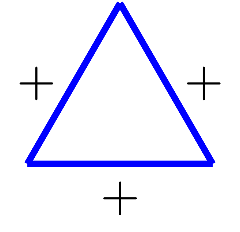
(a)

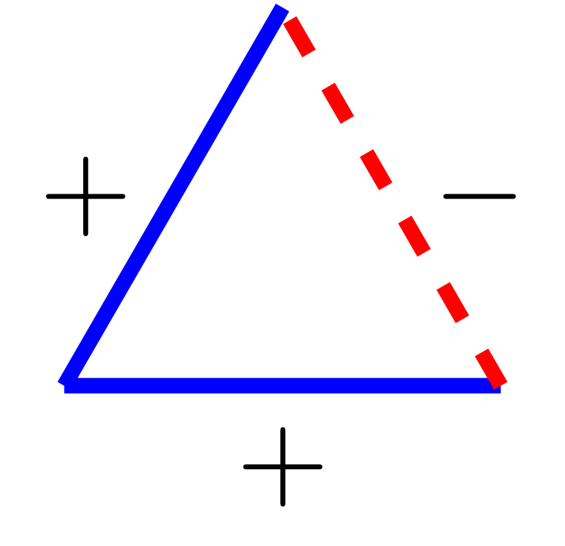
(b)

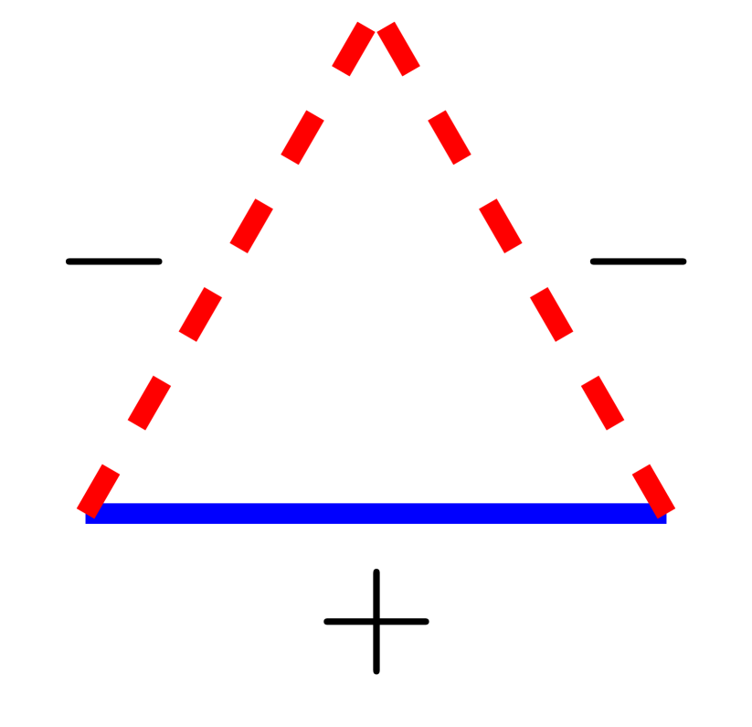
(c)

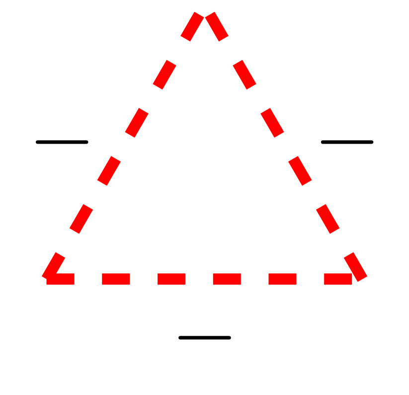
(d)

Figure 1: Heider’s triads corresponding to balanced (1(a) and 1(c)) and imbalanced (1(b) and 1(d)) states

When in every triangle these relations obey Heider’s rules mentioned above, the system is termed as balanced in Heider’s sense—which means that only triangles presented in Figures 1(a) and 1(c) are observed in the system.

The earlier studies have been devoted to triangular [10], diluted [11] and densified triangulations [12]; chains of nodes [13]; classical random graphs [14]; and complete graphs [15, 16].

Recently, reaching structural balance has been investigated with thermal noise modeled either with heat-bath [17, 15, 16] or Glauber dynamics [18, 19]. A more refined dynamics based on the indirect reciprocity mechanism on a complete graph has been studied in Reference [20].

In this paper, we continue studies of the influence of thermal noise on the possibility of reaching structural balance on Archimedean lattices containing triangles (see Figure 2). There are eleven Archimedean lattices [21], which contain only regular polygons allowing for covering plane with tiles and keeping the translational symmetry of the lattice. The systematic names of these lattices come from the number of edges in tiles attached to every lattice node sorted in the possibly lowest lexicographic order—for example, we call lattice presented in Figure 2(b) $(3^{2},4,3,4)$ and not $(4,3^{2},4,3)$ or $(4,3,4,3^{2})$. In this way, the square lattice is called $(4^{4})$, the triangular lattice is called $(3^{6})$, the honeycomb lattice is called $(6^{3})$ and kagomé lattice is called $(3,6,3,6)$.

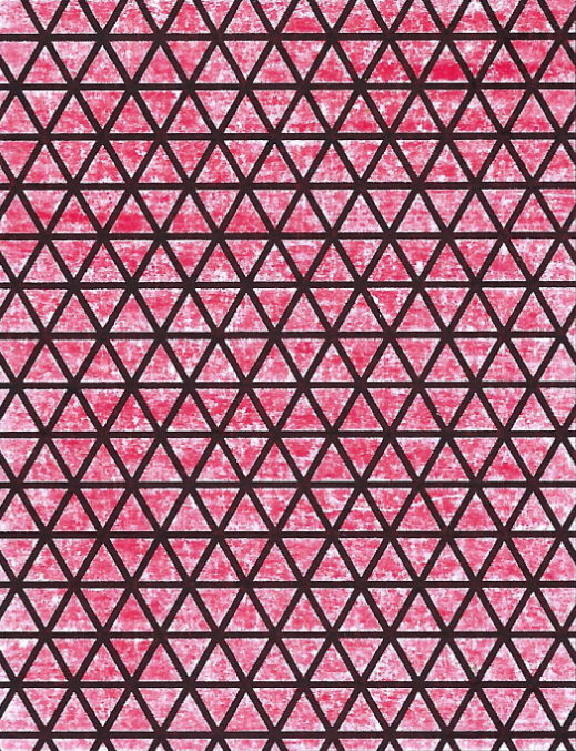
(a)

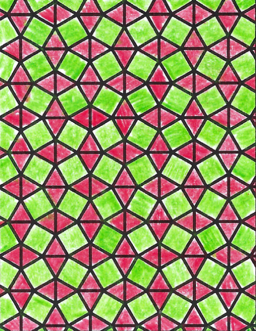
(b)

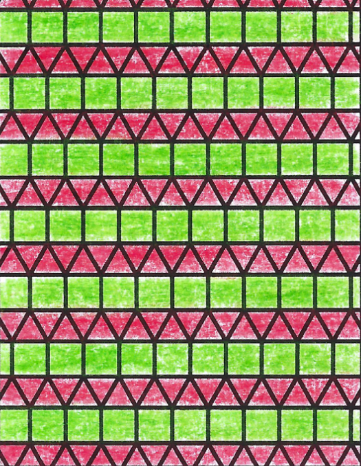
(c)

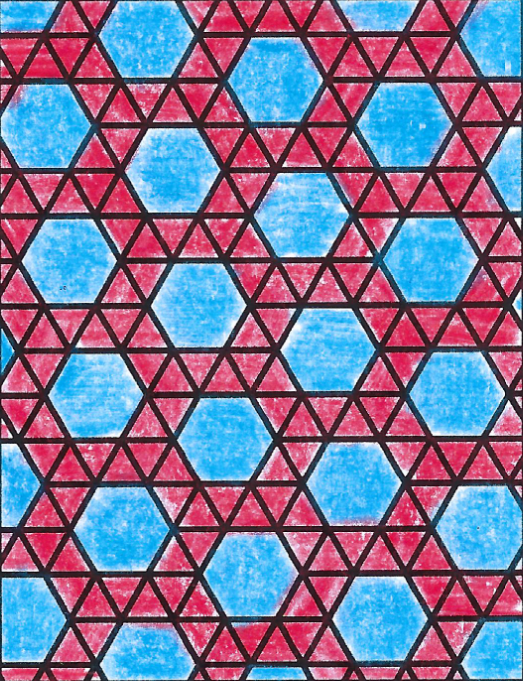
(d)

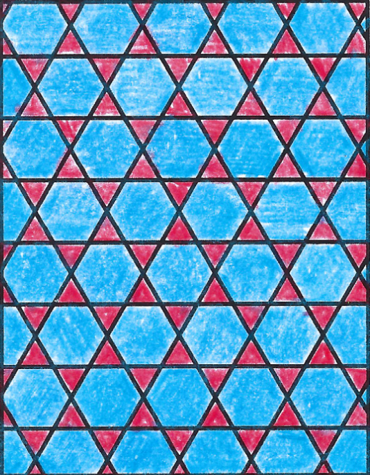
(e)

Figure 2: Shapes of the Archimedean lattices: (2(a)) $(3^{6})$; (2(b)) $(3^{2},4,3,4)$; (2(c)) $(3^{3},4^{2})$; (2(d)) $(3^{4},6)$; (2(e)) $(3,6,3,6)$

The Archimedean lattices investigated here are:

• separated triangles: kagomé—$(3,6,3,6)$ lattice, Figure 2(e);

• separated pairs of triangles: $(3^{2},4,3,4)$ lattice, Figure 2(b);

• chains of triangles: $(3^{3},4^{2})$ lattice, Figure 2(c);

• and segments of chains of triangles aligned on honeycomb lattice as a back-bone: maple leaf—$(3^{4},6)$ lattice, Figure 2(d).

Additionally, we inspect the system evolution for triangular $(3^{6})$ lattice (Figure 2(a)), diluted triangulations, and classical random graphs with mean node degree equal to $k=4$ and $k=5$, which also characterize the above-mentioned lattices. In Table 1 characteristics of the Archimedean lattices discussed in this work are collected. The social noise is modeled by the temperature parameter $T$ in the heat-bath scheme.

Our calculations are performed both with asynchronous and synchronous scheme. The former is known to reproduce properly the thermodynamic properties of systems in thermal equilibrium. The latter is justified if we intend to mimic the dynamics of opinions gathered periodically in polls. In this case, a respondent is not aware of the answers of other respondents during the same round. Such procedure of data collection has been applied in [22], to give an example.

The paper is organized as follows: in Section II we describe the methodology of studies (including the creation of adjacency matrices for the Archimedean lattices mentioned above, the heat-bath algorithm and calculation of the work function), Section III contains results of Monte Carlo simulations and Section IV is devoted to discussion of the obtained results and presentation of mathematical proof that structurally ordered phase is limited to $T=0$ on any two-dimensional lattice.

The paper is finalized with Appendix A showing lattices and adjacency matrices shapes and Appendix B with Fortran95 procedures for creating adjacency matrices for the lattices considered here.

II Methods

We keep the simulation methodology as presented for diluted/densified triangulations and classical random graphs [11, 12, 14]. In this approach (1), every link $x_{ij}$ represents friendly ($x_{ij}=+1$) or hostile ($x_{ij}=-1$) attitudes between actors $i$ and $j$, while (binary and symmetric) adjacency matrix $\mathbf{A}=[a_{ij}]$ elements

$$a_{ij}=\begin{cases}1&\iff i\text{ and }j\text{ are connected},\\ 0&\iff\text{otherwise},\end{cases}$$ (2)

define geometry of the lattice.

The Heider balance can be easily identified by checking the system work function [23, 24] per number of triangles $\Delta$ on lattice

$$U/\Delta\equiv-\frac{\operatorname{\mathrm{Tr}}[(\mathbf{A}\circ\mathbf{X})^{3}]}{\operatorname{\mathrm{Tr}}(\mathbf{A}^{3})},$$ (3)

where $\circ$ stands for the Hadamard product of the matrices and the matrix $\mathbf{X}=[x_{ij}]$. The system work function per triangle $U/\Delta$ is equal to $-1$ if and only if all triangles in the system are balanced.

II.1 Adjacency matrix representation of Archimedean lattices

In Appendix A in Figures 13(a), 10(a), 11(a), 12(a) and 9(a) the equivalents of the lattice shapes presented in Figure 2 are mapped onto distorted triangular lattices embedded in square lattices. The lattice edges are printed in thick solid black lines, while the underlying triangular lattice is presented in thin solid blue lines. The ‘unit cell’ is marked with a green dashed line. The periodic boundary conditions are assumed, and replicas of ‘elementary cell’ are marked with dotted cyan lines.

The Fortran procedures providing $\mathbf{A}$ for considered lattices are presented in Appendix B. Independently of the considered lattice, the module ‘par’ (see LABEL:lst:module-par in Appendix B) is required to define the linear size of the system $W$ and the lattice connectivity $k$.

Table 1: Characteristics of some Archimedean lattices. The second column indicates the lattice connectivity $k$. References to figures showing lattices’ shapes (and their shapes embedded in a distorted triangular lattice) are given in the third and the fourth columns. Figures showing the shapes of the adjacency matrix $\mathbf{A}$ are indicated in the fifth column. In the sixth column the labels of listings supplying $\mathbf{A}$ are listed

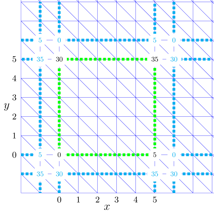
(a)

(b)

Figure 9: Triangular $(3^{6})$ lattice, $k=6$, (9(a)) $N=W^{2}$ nodes at and inside green square are labeled as $i=0,\cdots,W^{2}-1$, $i=x+Wy$, $x,y\in\{0,1,2,\cdots,W-1\}$, $W=6$ (9(b)) and its adjacency matrix

lattice	$k$	shape	shape in Appendix A	matrix $\mathbf{A}$ in Appendix A	subroutine in Appendix B
$(3^{6})$	6	Figure 2(a)	Figure 9(a)	Figure 9(b)	LABEL:lst:code-triangular
$(3^{2},4,3,4)$	5	Figure 2(b)	Figure 10(a)	Figure 10(b)	LABEL:lst:code-tri2al33434
$(3^{3},4^{2})$	5	Figure 2(c)	Figure 11(a)	Figure 11(b)	LABEL:lst:code-al33344
$(3^{4},6)$	5	Figure 2(d)	Figure 12(a)	Figure 12(b)	LABEL:lst:code-tri2mapleleaf
$(3,6,3,6)$	4	Figure 2(e)	Figure 13(a)	Figure 13(b)	LABEL:lst:code-tri2kagome

II.2 Heat-bath

The social noise level is mimicked by the temperature $T$ introduced in the probabilities of setting a hostile or friendly relation between actors. If $a_{ij}\neq 0$ then evolution of the link between nodes $i$ and $j$ of value $x_{ij}$ is given by

$$x_{ij}(t+1)=\begin{cases}+1&\text{ with probability }p_{ij}(t),\\ -1&\text{ with probability }[1-p_{ij}(t)],\end{cases}$$ (4a)

where

$$p_{ij}(t)=\frac{\exp[\beta\xi_{ij}(t)]}{\exp[\beta\xi_{ij}(t)]+\exp[-\beta\xi_{ij}(t)]},$$ (4b)

$$\beta=1/T$$ (4c)

and

$$\xi_{ij}(t)=\sum_{k}a_{ik}x_{ik}(t)\cdot a_{kj}x_{kj}(t).$$ (4d)

II.3 Calculations of $U(T)$

An ergodic Markov chain based on repeating local steps done with the heat-bath transition probability

$$p(A\rightarrow B)=\frac{e^{-\beta E_{B}}}{\sum_{C}e^{-\beta E_{C}}}$$ (5)

leads to a stationary state with the partition function

$$Z=\sum_{C}e^{-\beta E_{C}}.$$ (6)

For one triad, we have $2^{3}$ microscopic states $C$, four of them with energy $U=-1$ and four with energy $U=+1$; hence the partition function is

$$Z_{1}=\sum_{C}\exp(-\beta E_{C})=8\cosh(\beta),$$ (7)

and the mean value of energy is

$$U_{1}=-\frac{d}{d\beta}\ln Z_{1}=-\tanh(\beta).$$ (8)

For two triads with a common link, we have $2^{5}$ microscopic states. The energy spectrum contains eight states of energy equal $-2$, eight states of energy equal $+2$, and sixteen states of energy equal zero. The direct summation over these states gives the partition function $Z_{2}=Z_{1}^{2}$. Accordingly,

$$U_{2}=2U_{1}.$$ (9)

Figure 3: Chain of triangles appearing in $(3^{3},4^{2})$ lattice

For a chain of triangles shown in Figure 3, we can distinguish two kinds of links: internal (dashed) and closing (solid) ones. For each configuration of internal links, two states of each triad are possible, with opposing energies of this triad: $-1$ for a balanced triad, and $+1$ for an imbalanced triad. The energy of the triad is determined by the state of the third, closing link in this triad. Summarizing, the partition function of the chain includes:

• all configurations of internal links;

• two states of each closing link, with opposite energies, for each triad.

In this sense, the energies of the configurations depend only on the states of closing links,

$$Z_{N}=\sum_{i}\sum_{c}\exp(-\beta E(i,c))=2^{N}[2\cosh(\beta)]^{N},$$ (10)

where $i$ and $c$ are related to the states of internal and closing links, respectively. As a consequence, the energy per one triangle is equal to $-\tanh(\beta)$ again.

III Results

For all the considered lattices, the initial state of each of the links $x_{ij}$ is chosen randomly to be $+1$ or $-1$ with equal probabilities, so that $U/\Delta\approx 0$ at time $t=0$. Then, one of the two update procedures, synchronous or asynchronous, is applied for $t_{\text{max}}$ time steps, as given by Equation 4. In the case of the synchronous updating scheme, in one time step all links undergo this procedure simultaneously so that a new matrix $\mathbf{X}$ is created, which then replaces the old matrix before the next time step is performed. In the asynchronous approach, a single link is chosen randomly for an attempted update and its new value is determined instantly from Equation 4; in one time step this procedure is repeated as many times as the total number of links, which means that statistically each link is taken into account once in a time step. In both cases, the first 10% of the performed time steps are not taken into account when calculating the results presented below, so that the system can relax from the initial state. For most calculations $t_{\text{max}}=10^{4}$, but in some cases it is larger for $T<1$, as described below. In addition, all simulations are repeated 100 times and the mean value over those simulations is denoted by $\langle\cdots\rangle$.

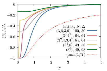
(a)

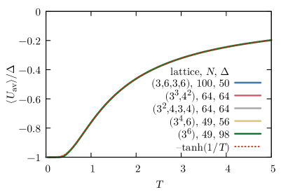
(b)

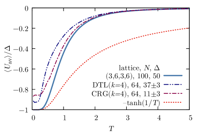
(c)

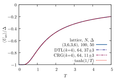
(d)

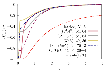
(e)

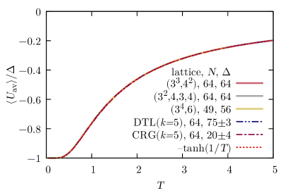
(f)

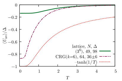
(g)

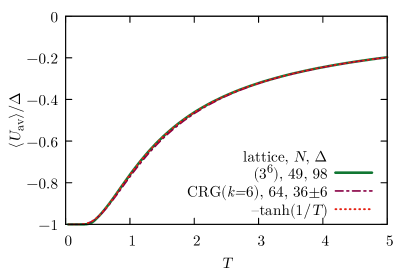
(h)

Figure 4: $\langle U_{\text{av}}\rangle/\Delta$ for synchronous (4(a), 4(c), 4(e), 4(g)), and asynchronous (4(b), 4(d), 4(f), 4(h)) update scheme. Nodes degree (on average, for the diluted triangular lattice and classical random graphs) $k=4$ (4(c), 4(d)), $k=5$ (4(e), 4(f)), $k=6$ (4(g), 4(h))

The energy per triangle defined in Equation 3 is therefore calculated in the final 90% of the time steps and then averaged to find $U_{\text{av}}$, and then averaged again over all the simulations performed. The results, denoted as $\langle U_{\text{av}}\rangle/\Delta$ are presented in LABEL:{fig:U_vs_T} as a function of temperature $T$, together with the curve given by

$$U/\Delta=-\tanh(1/T),$$ (11)

corresponding to the theoretical results of Section II.3.

The two approaches used in our calculations, synchronous and asynchronous, produce results that differ significantly at lower $T$. Figure 4(a) shows that the synchronous updating leads to $\langle U_{\text{av}}(T)\rangle/\Delta$ dependencies which are unique to each of the discussed Archimedean lattices. In the low-temperature limit, we observe perfectly balanced states, $\langle U_{\text{av}}\rangle/\Delta=-1$, in the $(3,6,3,6)$, $(3^{3},4^{2})$ and $(3^{4},6)$ lattices, but the decrease of energy with decreasing temperature occurs along a different curve for each of those lattices, and in all cases the values of the work function per triangle remain significantly larger than $-\tanh(1/T)$. On the other hand, only a slight decrease in the work function is found for the triangular lattice $(3^{6})$ and somewhat larger, to $\langle U_{\text{av}}(T\to 0)\rangle/\Delta\approx-0.5$, for the $(3^{2},4,3,4)$ lattice. For the asynchronous updating, the results in Figure 4(b) prove that for all types of the considered Archimedean lattices the temperature dependence of the work function per triad is exactly the same and identical to the theoretically predicted $U/\Delta=-\tanh(1/T)$.

For comparison, we match the Archimedean lattices with the corresponding diluted triangular lattices (DTL) [12] and classical random graphs (CRG) [14] having the same average node degree $k=4$, $5$, or $6$ as the connectivity of the considered Archimedean lattices. The only Archimedean lattice discussed here with $k=4$ is $(3,6,3,6)$ and for synchronous updating DTL and CRG of the same $k$ reveal similar but not identical characteristics, with non-perfect balance $\langle U_{\text{av}}(T)\rangle/\Delta\approx-0.9$ at $T\to 0$ as visible in Figure 4(c). It should be noted, though, that the random nature of the DTL and CRG graphs means that the simulations are performed on lattices with the same average node degree and number of nodes, but with different structure of connections (graph egdes) which results, among other things, in the number of triads in those lattices that is not constant in all simulations but found to be $\Delta=37\pm 3$ for DTL or $\Delta=11\pm 3$ for CRG, with $N=64$ in both cases. For $k=5$ (Figure 4(e)) and $k=6$ (Figure 4(g)) with synchronous updating the results for DTL and CRG are similar to those for $k=4$, which also means that they are not exactly in line with those for Archimedean lattices, in particular in the case of $(3^{2},4,3,4)$ lattice where the balanced state is not observed even in the low-temperature limit. At higher $T$, the results for all Archimedean, DTL and CRG lattices agree. For asynchronous updating, the results obtained for DTL and CRG at $k=4,5,6$ and presented in Figures 4(d), 4(f) and 4(h) do not differ from those of Archimedean lattices.

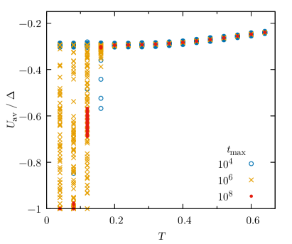
(a)

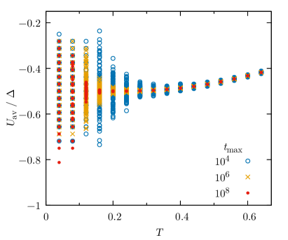
(b)

Figure 5: Values of $U_{\text{av}}/\Delta$ obtained in 100 simulations for each temperature $T$, for various simulation times $t_{\text{max}}=10^{4}$, $10^{6}$ and $10^{8}$, for (5(a)) $(3^{4},6)$ and (5(b)) $(3^{2},4,3,4)$ lattice and synchronous scheme of link updates

The dispersion of the values obtained in 100 simulations is usually relatively small, especially when asynchronous updating is applied. In most cases, it is also true for synchronous updating, except for the $(3^{2},4,3,4)$ and $(3^{4},6)$ lattices at $T<1$ where it was required to perform $t_{\text{max}}=10^{8}$ time steps, and for DTL and CRG lattices where $t_{\text{max}}=10^{6}$ was used. In particular in the case of $(3^{4},6)$ lattice shorter simulations do not allow us to see that the balanced state is achieved at $T\to 0$, as visible in Figure 5(a) showing the values $U_{\text{av}}/\Delta$ obtained in all performed simulations. Figure 5(b) confirms that on the $(3^{2},4,3,4)$ lattice the balanced state is not observed even in the low-temperature limit, and additionally the values of the work function obtained in the simulations performed are quantized and distributed over a relatively long interval. The values of the work function observed at the lowest $T$ are spaced in the intervals of $2/\Delta$, which corresponds to the difference related to the energetically nearest states. The same quantization of the work function applies for any other two-dimensional lattice that contains triangles as it is associated with changing a single term ($x_{ij}x_{jk}x_{ik}$—where $i$, $j$, $k$ are triangle vertices) in sum in nominator of Equation 3 from $+1$ to $-1$ (or vice versa).

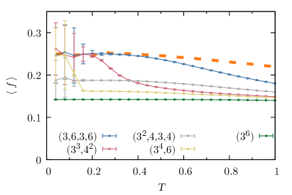
(a)

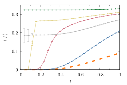
(b)

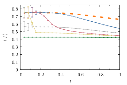
(c)

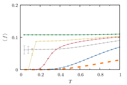
(d)

Figure 6: Thermal evolution (in the low temperature limit $T<1$) of fractions of triads presented in Figure 1 in the case of asynchronous updating and different Archimedean lattices. The panels (6(a)), (6(b)), (6(c)), and (6(d)) correspond to the triangles presented in Figures 1(a), 1(b), 1(c), and 1(d), respectively. The error bars show the standard deviation of the results in 100 simulations. Dashed line for asynchronous updating (common result for all lattices)

If any of the systems discussed is in the balanced state, it means that all triads are balanced, that is, they are in one of two possible configurations: with all positive links ($[+++]$, Figure 1(a)) or with one positive and two negative links ($[+--]$, Figure 1(c)). The fraction of triads of a given kind, $\langle f\rangle$, as a function of $T$ is shown in Figure 6. It reveals that in the cases where the balanced state is reached at $T\to 0$, about 25% of the triads are in the $[+++]$ configuration, and the rest are in the $[+--]$ state. However, in that limit (only for $T<0.2$) those fractions vary substantially among the simulations, as shown by the error bars indicating the standard deviation, which is also the case for the $(3^{2},4,3,4)$ lattice which does not reach the balanced state and for all triads in that case including $[++-]$ (Figure 1(b)) and $[---]$ (Figure 1(d)). On the other hand, the $(3^{6})$ triangular lattice produces almost identical results in all simulations. In the balanced state observed in the low-temperature limit, the fractions of triads obtained using the asynchronous updating scheme (dashed lines in Figure 6) are the same as for the balanced state reached with synchronous updating. However, in the case of asynchronous updating the increasing temperature causes much slower decrease of the number of balanced triads than for synchronous approach, which is also visible in slower increase of the work function with increasing $T$.

IV Discussion

Here we show that the Heider model (1) on a two-dimensional lattice with the asynchronous updates is equivalent to a one-dimensional Ising model with the nearest-neighbor interactions.

Let us apply the following transformation, where $s_{i}=-1$,

$$x^{\prime}_{ij}=s_{i}x_{ij},$$ (12)

to all links incident with the node $i$. The total energy of the system (1) remains the same $E_{A^{\prime}}=E_{A}$. The gauge transformation (12) leaves the spin products $x_{ij}x_{jk}\ldots x_{si}$ unchanged in any closed loop. The transformation (12) can be repeated for any node of the lattice. The configurations obtained in this way form an equivalence class with the same energy. Let $N$ be the number of nodes. It is easy to see that each equivalence class contains $2^{N-1}$ configurations since one can apply the transformation (12) to $(N-1)$ nodes. Applying it to the $N$-th node would undo all changes as each spin $x_{ij}$ would be multiplied twice $s_{i}x_{ij}s_{j}$. Degeneracy can be removed by fixing values $x_{ij}$ on any spanning tree of the lattice, for example by assigning all edges of the tree the value one: $x_{ij}=1$. The spanning tree has $N-1$ edges, so fixing the gauge completely eliminates degeneracy. Once the gauge is fixed, the partition function (6) can be reduced to

$$Z=2^{N-1}\sum_{a}e^{-\beta E_{a}},$$ (13)

where $a$ are configurations of $x_{ij}$ for all edges except those which were fixed to one on the spanning tree. We will illustrate this equivalence in detail on a triangular lattice with twisted boundary conditions, as shown in Figure 7, but it can be easily modified for any two-dimensional lattice.

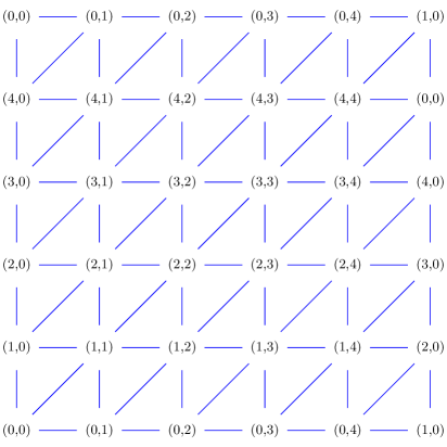
Figure 7: An example of a triangular lattice with a toroidal topology with twisted boundary conditions. The lattice has $N=25$ nodes, indexed by $(i,j)$, with $i=0,\ldots,4$ and $j=0,\ldots,4$. It has $\Delta=50$ triangles and $L=75$ links. The twisted boundary condition is encoded in a shift by one in the coordinate $j$ between the first and the last columns

Let us introduce a gauge fixing as shown in Figure 8: $x_{ij}=1$ for all edges $ij$ on the line drawn in red.

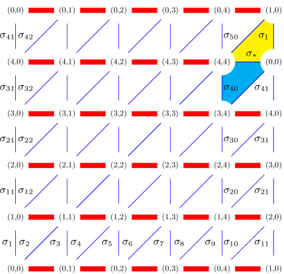
Figure 8: Gauge fixing: for all red edges $x_{ij}=1$. Any white triangle has two free edges, for which $x_{ij}=\pm 1$. There are only two triangles with three free edges. They are drawn in yellow and turquoise

Let us label the values of spins for the free links (which do not belong to the gauge tree) as $\sigma_{1},\ldots,\sigma_{50}$ as shown in Fig. 8, and denote the value of $\sigma$ on the link $(4,4)-(0,0)$ by $\sigma_{*}$. We can write the partition function (6) for this gauge fixing as

$$Z=2^{N-1}(Z_{+}+Z_{-}),$$ (14)

where $Z_{+}$ and $Z_{-}$ are sums over configurations with $\sigma_{*}=+1$ and $\sigma_{*}=-1$, respectively. It is easy to see that

$$Z_{+}=\sum_{\sigma}e^{\beta\sum_{i=1}^{50}\sigma_{i}\sigma_{i+1}},$$ (15)

where $\sigma_{51}=\sigma_{1}$. This is a partition function of the one-dimensional nearest-neighbor Ising model with periodic boundary conditions. For $\sigma_{*}=-1$ we have

$$Z_{-}=\sum_{\sigma}e^{\beta(\sum_{i=1}^{50}\sigma_{i}\sigma_{i+1}-E)},$$ (16)

where $E=2\sigma_{39}\sigma_{40}+2\sigma_{50}\sigma_{1}$. Up to the last term $E$, $Z_{-}$ is also equal to the partition function of the one-dimensional Ising model. This term introduces some finite size corrections which can be neglected when the size $n\times n$ of the lattice increases $n\to\infty$, so we see that for large lattices the original model is mapped into a one-dimensional Ising model on a chain of length $2n$. Energy per node for the Ising chain is known to be $-\tanh\beta$, so therefore in the Heider model with asynchronous update scheme energy per triangle should reproduce this result $U/\Delta\rightarrow-\tanh\beta$ in the limit $n\to\infty$. This is not the case for synchronous update scheme which violates the detailed balance condition.

Appendix A Archimedean lattices mapped into square lattice and the shapes of their adjacency matrices

In Figures 13(a), 10(a), 11(a), 12(a) and 9(a) shapes of Archimedean lattices embedded in a distorted triangular lattice are presented for kagomé, $(3^{2},4,3,4)$, $(3^{3},4^{2})$, maple-leaf, and triangular lattices, respectively.

In Figures 13(b), 10(b), 11(b), 12(b) and 9(b) examples of adjacency matrices associated with lattices presented in Figures 13(a), 10(a), 11(a), 12(a) and 9(a) are displayed.

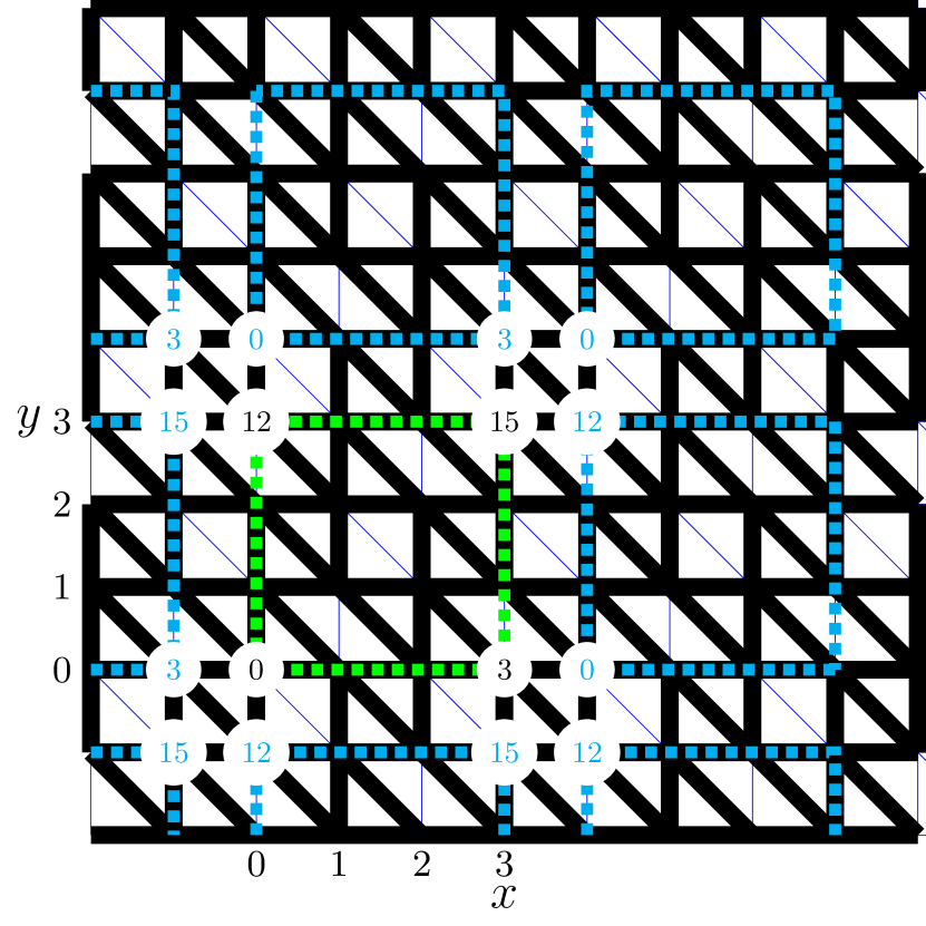
(a)

(b)

Figure 10: Archimedean $(3^{2},4,3,4)$ lattice, $k=5$, (10(a)) $N=W^{2}$ nodes at and inside green square are labeled as $i=0,\cdots,W^{2}-1$, $i=x+Wy$, $x,y\in\{0,1,2,\cdots,W-1\}$, $W=4$ (10(b)) and its adjacency matrix

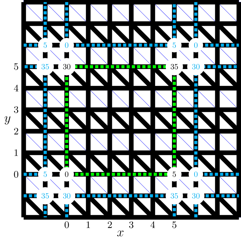
(a)

(b)

Figure 11: Archimedean $(3^{3},4^{2})$ lattice, $k=5$, (11(a)) $N=W^{2}$ nodes at and inside green square are labeled as $i=0,\cdots,W^{2}-1$, $i=x+Wy$, $x,y\in\{0,1,2,\cdots,W-1\}$, $W=6$ (11(b)) and its adjacency matrix

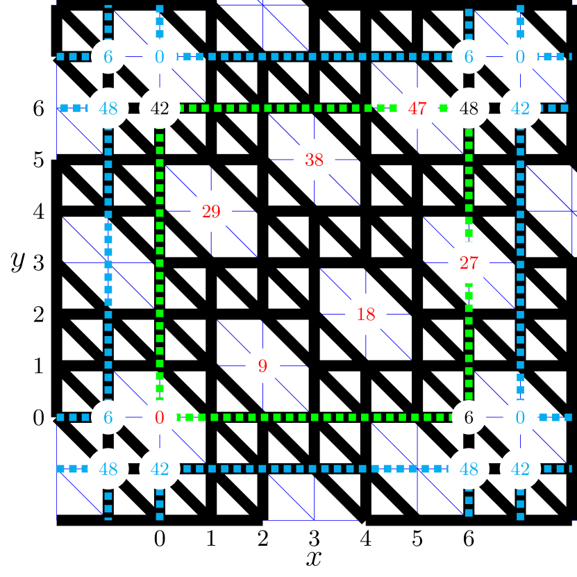
(a)

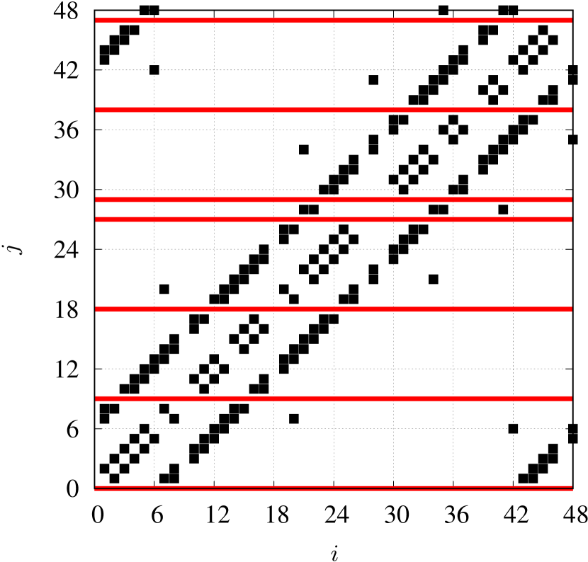
(b)

Figure 12: Maple leaf $(3^{4},6)$ lattice, $k=5$, (12(a)) $N=W^{2}$ nodes at and inside green square are labeled as $i=0,\cdots,W^{2}-1$, $i=x+Wy$, $x,y\in\{0,1,2,\cdots,W-1\}$, $W=7$ (12(b)) and its adjacency matrix

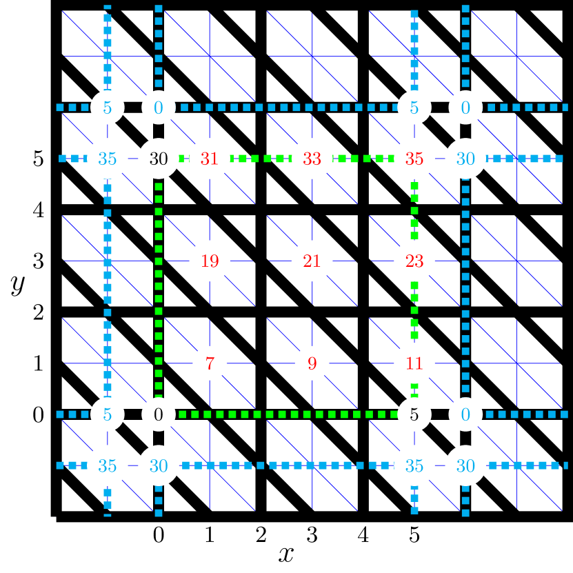
(a)

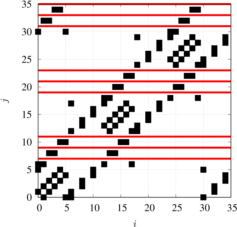
(b)

Figure 13: Archimedean $(3,6,3,6)$ lattice (kagomé lattice), $k=4$, (13(a)) $N=W^{2}$ nodes at and inside green square are labeled as $i=0,\cdots,W^{2}-1$, $i=x+Wy$, $x,y\in\{0,1,2,\cdots,W-1\}$, $W=6$ (13(b)) and its adjacency matrix

Appendix B Listings

LABEL:lst:module-par presents Fortran module defining constant parameters for the subroutines supplying the adjacency matrix $\mathbf{A}$. The integer variable Z corresponds to the network connectivity $k$. The integer variable W represents the linear size of the underlying square lattice in which the distorted triangles are embedded. Then, the integer variable N is equal to the square of W. To ensure the possibility of wrapping the lattice according to the assumed periodic boundary condition, its value must be a multiple of 4 for $(3^{2},4,3,4)$ and 7 for $(3^{4},6)$. The other lattices are presented for W=6, however for $(3^{3},4^{2})$ and $(3,6,3,6)$ any even number is suitable, while there are no restrictions in the case of the triangular lattice $(3^{6})$.

LABEL:lst:code-triangular, LABEL:lst:code-al33344, LABEL:lst:code-tri2kagome, LABEL:lst:code-tri2mapleleaf and LABEL:lst:code-tri2al33434 contain Fortran subroutines computing the adjacency matrix $\mathbf{A}$ for triangular, $(3^{2},4,3,4)$, $(3^{3},4^{2})$, $(3^{4},6)$, and $(3,6,3,6)$, respectively. Subroutines tri_2_al33434 (LABEL:lst:code-tri2al33434), tri_2_maple_leaf (LABEL:lst:code-tri2mapleleaf), tri_2_kagome (LABEL:lst:code-tri2kagome) for the $(3^{2},4,3,4)$, $(3^{3},6)$, $(3,6,3,6)$ lattices, respectively, require earlier preparation of adjacency matrix $\mathbf{A}$ as for triangular lattices using the subroutine given in LABEL:lst:code-triangular. The adjacency matrix $\mathbf{A}$ is returned in the matrix variable A. The local matrix variable nn (if used) stores labels of $k$ neighbors of the sites in the lattice.

Listing 1: Module including parameters

⬇

1MODULE par

2INTEGER, PARAMETER :: Z=5, W=7, N=W*W

3END MODULE

Listing 2: Subroutine for triangular $(3^{6})$ lattice

⬇

1SUBROUTINE triangular(A)

2!! -------------------------------------------

3USE par

4IMPLICIT NONE

5INTEGER, DIMENSION(0:N-1,0:Z-1) :: nn

6INTEGER, DIMENSION(0:N-1,0:N-1) :: A

7INTEGER :: i, j

8!! -------------------------------------------

9DO i=0, N-1

10 nn(i,0) = MOD(N+i -W ,N)

11 nn(i,1) = MOD(N+i -W+1,N)

12 nn(i,2) = MOD(N+i -1 ,N)

13 nn(i,3) = MOD(N+i +1 ,N)

14 nn(i,4) = MOD(N+i +W-1,N)

15 nn(i,5) = MOD(N+i +W ,N)

16 IF(MOD(i,W)==0) THEN

17 nn(i,2) = MOD(N+W+i -1 ,N)

18 nn(i,4) = MOD(N+W+i +W-1,N)

19 ENDIF

20 IF(MOD(i+1,W)==0) THEN

21 nn(i,1) = MOD(N-W+i -W+1,N)

22 nn(i,3) = MOD(N-W+i +1 ,N)

23 ENDIF

24ENDDO

25!! -------------------------------------------

26A=0

27DO i=0,N-1

28DO j=0,Z-1

29 A(i,nn(i,j))=1

30ENDDO

31ENDDO

32!! -------------------------------------------

33END SUBROUTINE triangular

Listing 3: Subroutine for Archimedean $(3^{2},4,3,4)$ lattice

⬇

1SUBROUTINE tri_2_al33434(A)

2USE par

3IMPLICIT NONE

4INTEGER, DIMENSION(0:N-1,0:Z-1) :: nn

5INTEGER, DIMENSION(0:N-1,0:N-1) :: A

6INTEGER :: i, x ,y

7!! -------------------------------------------

8!! neighbors on triangular lattice

9DO i=0, N-1

10 nn(i,0) = MOD(N+i -W ,N)

11 nn(i,1) = MOD(N+i -W+1,N)

12 nn(i,2) = MOD(N+i -1 ,N)

13 nn(i,3) = MOD(N+i +1 ,N)

14 nn(i,4) = MOD(N+i +W-1,N)

15 nn(i,5) = MOD(N+i +W ,N)

16 IF(MOD(i,W)==0) THEN

17 nn(i,2) = MOD(N+W+i -1 ,N)

18 nn(i,4) = MOD(N+W+i +W-1,N)

19 ENDIF

20 IF(MOD(i+1,W)==0) THEN

21 nn(i,1) = MOD(N-W+i -W+1,N)

22 nn(i,3) = MOD(N-W+i +1 ,N)

23 ENDIF

24ENDDO

25!! -------------------------------------------

26!! adjacency matrix for (3^2,4,3,4) lattice:

27DO x=0,W-1

28DO y=0,W-1

29 i=x+y*W

30 IF(MOD(x,W).EQ.0 .AND. MOD(y,W).EQ.0)

31 A(i,nn(i,1))=0

32 IF(MOD(x,W).EQ.1 .AND. MOD(y,W).EQ.0)

33 A(i,nn(i,5))=0

34 IF(MOD(x,W).EQ.2 .AND. MOD(y,W).EQ.0)

35 A(i,nn(i,1))=0

36 IF(MOD(x,W).EQ.3 .AND. MOD(y,W).EQ.0)

37 A(i,nn(i,5))=0

38

39 IF(MOD(x,W).EQ.0 .AND. MOD(y,W).EQ.1)

40 A(i,nn(i,4))=0

41 IF(MOD(x,W).EQ.1 .AND. MOD(y,W).EQ.1)

42 A(i,nn(i,0))=0

43 IF(MOD(x,W).EQ.2 .AND. MOD(y,W).EQ.1)

44 A(i,nn(i,4))=0

45 IF(MOD(x,W).EQ.3 .AND. MOD(y,W).EQ.1)

46 A(i,nn(i,0))=0

47

48 IF(MOD(x,W).EQ.0 .AND. MOD(y,W).EQ.2)

49 A(i,nn(i,5))=0

50 IF(MOD(x,W).EQ.1 .AND. MOD(y,W).EQ.2)

51 A(i,nn(i,1))=0

52 IF(MOD(x,W).EQ.2 .AND. MOD(y,W).EQ.2)

53 A(i,nn(i,5))=0

54 IF(MOD(x,W).EQ.3 .AND. MOD(y,W).EQ.2)

55 A(i,nn(i,1))=0

56

57 IF(MOD(x,W).EQ.0 .AND. MOD(y,W).EQ.3)

58 A(i,nn(i,0))=0

59 IF(MOD(x,W).EQ.1 .AND. MOD(y,W).EQ.3)

60 A(i,nn(i,4))=0

61 IF(MOD(x,W).EQ.2 .AND. MOD(y,W).EQ.3)

62 A(i,nn(i,0))=0

63 IF(MOD(x,W).EQ.3 .AND. MOD(y,W).EQ.3)

64 A(i,nn(i,4))=0

65ENDDO

66ENDDO

67END SUBROUTINE tri_2_al33434

Listing 4: Subroutine for Archimedean $(3^{3},4^{2})$ lattice

⬇

1SUBROUTINE al_33344(A)

2!! -------------------------------------------

3USE par

4IMPLICIT NONE

5INTEGER, DIMENSION(0:N-1,0:Z-1) :: nn

6INTEGER, DIMENSION(0:N-1,0:N-1) :: A

7INTEGER :: i, j, x, y

8!! -------------------------------------------

9DO y=0,W-1,2

10DO x=0,W-1

11 i=x+y*W

12 nn(i,0) = MOD(N+i -1 ,N)

13 nn(i,1) = MOD(N+i +1 ,N)

14 nn(i,2) = MOD(N+i -W ,N)

15 nn(i,3) = MOD(N+i +W ,N)

16 nn(i,4) = MOD(N+i +W-1,N)

17 IF(MOD(i,W)==0) THEN

18 nn(i,0) = MOD(N+W+i -1 ,N)

19 nn(i,4) = MOD(N+W+i +W-1,N)

20 ENDIF

21 IF(MOD(i+1,W)==0) THEN

22 nn(i,1) = MOD(N-W+i +1,N)

23 ENDIF

24ENDDO

25ENDDO

26!! -------------------------------------------

27DO y=1,W-1,2

28DO x=0,W-1

29 i=x+y*W

30 nn(i,0) = MOD(N+i -1 ,N)

31 nn(i,1) = MOD(N+i +1 ,N)

32 nn(i,2) = MOD(N+i -W ,N)

33 nn(i,3) = MOD(N+i +W ,N)

34 nn(i,4) = MOD(N+i -W+1,N)

35 IF(MOD(i,W)==0) THEN

36 nn(i,0) = MOD(N+W+i -1,N)

37 ENDIF

38 IF(MOD(i+1,W)==0) THEN

39 nn(i,1) = MOD(N-W+i +1,N)

40 nn(i,4) = MOD(N-W+i -W+1,N)

41 ENDIF

42ENDDO

43ENDDO

44!! -------------------------------------------

45A=0

46DO i=0,N-1

47DO j=0,Z-1

48 A(i,nn(i,j))=1

49ENDDO

50ENDDO

51!! -------------------------------------------

52END SUBROUTINE al_33344

Listing 5: Subroutine for maple leaf $(3^{3},6)$ lattice

⬇

1SUBROUTINE tri_2_maple_leaf(A)

2!! -------------------------------------------

3USE par

4IMPLICIT NONE

5INTEGER, DIMENSION(0:N-1,0:N-1) :: A

6INTEGER :: i, j, k, x, y

7!! -------------------------------------------

8DO y=0,W-1

9DO k=1,S

10 x = MOD(2*y+7*k,W)

11 i = x + W*y

12 DO j=0,N-1

13 A(i,j)=0

14 A(j,i)=0

15 ENDDO

16ENDDO

17ENDDO

18!! -------------------------------------------

19END SUBROUTINE tri_2_maple_leaf

Listing 6: Subroutine for kagomé $(3,6,3,6)$ lattice

⬇

1SUBROUTINE tri_2_kagome(A)

2!! -------------------------------------------

3USE par

4IMPLICIT NONE

5INTEGER, DIMENSION(0:N-1,0:N-1) :: A

6INTEGER :: i, j, x, y

7!! -------------------------------------------

8DO y=1,W,2

9DO x=1,W,2

10 i=x+W*y

11 DO j=0,N-1

12 A(i,j)=0

13 A(j,i)=0

14 ENDDO

15ENDDO

16ENDDO

17!! -------------------------------------------

18END SUBROUTINE tri_2_kagome