Linear Submodular Maximization with Bandit Feedback

Abstract

Submodular optimization with bandit feedback has recently been studied in a variety of contexts. In a number of real-world applications such as diversified recommender systems and data summarization, the submodular function exhibits additional linear structure. We consider developing approximation algorithms for the maximization of a submodular objective function $f:2^{U}\to\mathbb{R}_{\geq 0}$, where $f=\sum_{i=1}^{d}w_{i}F_{i}$. It is assumed that we have value oracle access to the functions $F_{i}$, but the coefficients $w_{i}$ are unknown, and $f$ can only be accessed via noisy queries. We develop algorithms for this setting inspired by adaptive allocation algorithms in the best-arm identification for linear bandit, with approximation guarantees arbitrarily close to the setting where we have value oracle access to $f$. Finally, we empirically demonstrate that our algorithms make vast improvements in terms of sample efficiency compared to algorithms that do not exploit the linear structure of $f$ on instances of move recommendation.

1 Introduction

Submodular set functions satisfy a diminishing returns property that arises in many optimization problems in machine learning such as those involving coverage functions (Bateni et al., 2017), data summarization (Lin and Bilmes, 2011; Tschiatschek et al., 2014), facility location  (Lindgren et al., 2016), viral marketing in social networks (Kempe et al., 2003), and recommendation systems (Leskovec et al., 2007; El-Arini and Guestrin, 2011). A set function $f:2^{U}\to\mathbb{R}$ is submodular if for every $X\subseteq Y\subseteq U$ and for every $x\in U\setminus Y$, we have $f(X\cup\{x\})-f(X)\geq f(Y\cup\{x\})-f(Y)$. In addition, $f$ is often monotone, i.e., $f(Y)\geq f(X)$ for every $X\subset Y$. Among the most widely considered formulations is the NP-hard monotone submodular maximization problem with a cardinality constraint Nemhauser et al. (1978): Given budget $\kappa$, find $\arg\max_{|S|\leq\kappa}f(S)$. The setting of most existing work on SM is that we have value oracle access to $f$, and algorithms may query any subset $X\subset U$ and the value of $f(X)$ is returned.

However, in many applications it is not realistic to assume that we have value oracle access to $f$, but rather that we can only query $f$ approximately or subject to some noise (Kempe et al., 2003; Singla et al., 2016; Horel and Singer, 2016; Hassidim and Singer, 2017a; Parambath et al., 2018; Peng, 2021) Within this broad area of noisy access to $f$, one important line of work consider the development of algorithms for the special case that $f$ has additional linear structure (Yue and Guestrin, 2011; Yu et al., 2016; Chen et al., 2017; Hiranandani et al., 2020). In particular, the setting and problem is described below.

Definition 1 (Linear Submodular Maximization with a Cardinality Constraint (SM)).

Let $U$ be a universe of elements of size $n$. Suppose we have $d$ monotone and submodular functions denoted as $F_{i}:2^{U}\rightarrow\mathbb{R}$ for $i=1,2,...,d$. The objective function $f:2^{U}\rightarrow\mathbb{R}$ is a weighted sum of the $d$ submodular functions, i.e. $f(S)=\sum_{i=1}^{d}w_{i}F_{i}(S)=\textbf{F}^{T}(S)\textbf{w}$, where $\textbf{F}(S)=(F_{1}(S),F_{2}(S),...,F_{d}(S))^{T}$, $\textbf{w}=(w_{1},w_{2},...,w_{d})^{T}$, and $w_{i}\geq 0$ for any $i\in[d]$. SM is then defined to be, given budget $\kappa$, find $\arg\max_{|S|\leq\kappa}f(S)$.

Notice that $f$ is also monotone and submodular, since it is the linear sum of monotone submodular functions. It is assumed that we have value oracle access to each of the basis functions $F_{i}$, and we can query them on any subset $S\subseteq U$, but the weight vector $\textbf{w}=(w_{1},w_{2},...,w_{d})^{T}$ is unknown. We do not have oracle access to $f$, but we may make i.i.d. R-sub-Gaussian noisy queries to $f$ where the expectation is the true value of $f$. An important application of this setting is recommendation systems, which we will more thoroughly describe in Section 2. These assumptions on the structure of $f$ and noise fall into the well-studied linear bandit model (Soare et al., 2014; Xu et al., 2018), as we will explain in more detail in Section 2. The focus of existing work on SM in this setting is integrating linear bandit strategies and algorithms for SM together in order to select a subset $X\subseteq U$ over a series of iterations that minimizes regret (the online regret minimization setting) (Yue and Guestrin, 2011; Yu et al., 2016; Chen et al., 2017; Hiranandani et al., 2020). Existing works emphasize the online regret minimization setting, wherein the agent strives to select a solution set with high expected function values while exploring new sets.

In the online regret minimization setting, a solution set is selected at each iteration and some corresponding noisy feedback from $f$ is returned. It is assumed that there is a penalty to choosing a bad set, e.g. a set with low $f$ value is recommended to a user, and so a balance between exploration (sampling in order to better estimate w) and exploitation (choosing sets at each iteration, e.g. to recommend to a user, that are believed to be of high value) is used in order to select sets. On the other hand, an alternative to the regret minimization setting is that of the pure exploration linear bandit (Soare et al., 2014; Xu et al., 2018), where as few noisy samples as possible are taken in orders to arrive at a good solution quickly. We depart from existing literature on linear submodular bandit in that we do not use the online regret minimization setting, but instead make use of ideas from pure exploration linear bandit. More specifically, our goal is to provide a solution set with a PAC-style theoretical guarantee Even-Dar et al. (2002); Kalyanakrishnan et al. (2012), where the bandit algorithm identifies an $\epsilon$-optimal arm with probability at least $1-\delta$, in as few samples as possible. This type of problem has been previously studied in the submodular optimization literature by Singla et al. in the general case where $f$ does not have linear structure. But the linear structure of $f$ allows us to develop algorithms that make significantly fewer noisy samples (as will be demonstrated in Section 5), because we are able to learn the unknown vector w as more and more noisy samples are made.

In particular, the contributions of our paper are as follows: (i) We propose and analyze the algorithm Linear Greedy (LG), which is inspired by the standard greedy algorithm, but proceeds as $\kappa$ rounds of best-arm-identification problems in the linear bandit setting. We prove that the exact function value of the output solution set of LG $S$ is arbitrarily close to the optimal approximation guarantee of $1-1/e$ for cardinality constrained submodular maximization (Nemhauser et al., 1978). In addition, LG chooses an optimal sample allocation strategy, and we prove a bound on the total number of noisy samples required by LG. (ii) We next propose and analyse the algorthm Linear Threshold Greedy (LinTG) which is based on the threshold greedy algorithm of Badanidiyuru and Vondrák (2014), but we propose a new linear bandit strategy in a novel setting that is distinct from best-arm-identification. LinTG is more efficient compared to LG from an algorithmic perspective, but additionally the linear bandit strategy itself is more efficient in several ways. Similar to LG, LinTG is proven to return a solution set $S$ that is arbitrarily close to $1-1/e$. (iii) Finally, we compare our algorithms to several alternative approaches to this problem on instances of movie recommendation. We find that our algorithms make significant improvements in terms of sample complexity.

1.1 Related Work

There has been a great line of work on noisy submodular maximization Horel and Singer (2016); Hassidim and Singer (2017b); Crawford et al. (2019). Among these works, the most related setting assumes the noisy feedback is i.i.d $R$-sub-Gaussian, which is also referred to as bandit feedback Singla et al. (2016); Karimi et al. (2017). The problem is also referred to as submodular bandit, which is a specific type of combinatorial multi-armed bandit problem with the reward function assumed to be submodular Chen et al. (2017); Takemori et al. (2020); Hiranandani et al. (2020). The main focus of these works are regret minimization. Among the works studying submodular bandit, the linear submodular bandit is a specific problem with the same objective function as us Yue and Guestrin (2011); Takemori et al. (2020); Yu et al. (2016), i.e., the objective function $f$ can be expressed by the linear sum of known submodular functions with unknown weights. The problem was first introduced by Yue and Guestrin (2011), who studied the problem with the goal of regret minimization. Under this setting, the strategy is to explore new choices of the subsets while also exploiting previous samples to select good ones. Therefore, the algorithm should be encouraged to choose the sets with higher function values while the main focus of our paper is to study the linear submodular bandit under best-arm identification setting, where the objective is to find the best solution set in fewer queries. One obvious approach to this problem is to simply take sufficiently many noisy samples so that $f$ is approximated very closely for all sets that are to be queried, and then apply existing algorithms for SM on the approximation of $f$. The downsides of such an approach is that not only is it unnecessary to approximate $f$ so closely when making decisions during an algorithm, but this approach does not exploit the linear structure of $f$. A difficulty with such algorithms is that the large number of noisy samples can make such an approach impractical.

Another related line of work is the problem of identifying the best element in linear bandit (The arms are single elements in the universe.), which is first studied in Soare et al. (2014). The authors proposed static allocation strategies and adaptive strategies based on successive elimination. Later on, there are a large line of works that proposed more adaptive algorithms Xu et al. (2018); Degenne et al. (2020). Xu et al. (2018) proposed an algorithm named LinGap which is claimed to be fully adaptive and performed better than those in Soare et al. (2014). Degenne et al. (2020) proposed the first algorithm that is asymptotically optimal.

2 Preliminaries

In this section, we present the basic setup for our problem, including motivating examples, a description of the linear bandit setting, and related technical background that will be used for our algorithms. First, we provide some additional information about our problem formulation. We assume that the $l_{2}$ norm of w is bounded by $S$, and the $l_{2}$ norm of $\textbf{F}(s)$ is bounded by $L$ for any $s\in U$.

For any $S\subseteq U$ and $x\in U$, the sampling result of the marginal gain $\Delta f(S,x)$ is i.i.d $R$-sub-Gaussian with expectation $\Delta f(S,x)$. Let us denote the $t$-th independent samples of $\Delta f(S,x)$ as $\Delta f_{t}(S,x)$. We assume the noisy queries can be expressed as $\Delta f_{t}(S,x)=\sum_{i=1}^{d}w_{i}\Delta F_{i}(S,x)+\xi_{t}=\Delta\textbf{F}^{T}(S,x)\textbf{w}+\xi_{t}$, where $\xi_{t}$ are i.i.d zero-mean noise and $R$-sub-Gaussian. Therefore we have that $\mathbb{E}\Delta f_{t}(S,x)=\sum_{i=1}^{d}w_{i}\Delta F_{i}(S,x)=\Delta f(S,x)$. Linear submodular functions arise in a wide range of applications including recommender systems, weighted coverage, and facility location. Next, we describe the application of the recommender system as an example to illustrate our problem setting.

2.1 Motivating application: diversified recommender systems

In this application, the user examines the recommended list of $S$ of $\kappa$ items from the first item to the last, clicks on the first attractive item, and does not examine the rest. Herein, the submodular function is the expected total clicks from recommending the list of items. Suppose $F_{i}(S)$ denotes a submodular function quantifying the incorporation of topic $i$ within the recommended item set $S$ which is usually modeled by the probabilistic coverage model Yue and Guestrin (2011); Hiranandani et al. (2020), and that $w_{i}$ is the preference of the user towards the topic $i$ and is unknown to the algorithm. Then $f(S)$ is defined as $f(S)=\sum_{i\in d}w_{i}F_{i}(S)$. By definition, we have that $\sum_{i}w_{i}=1$. Therefore, $||\textbf{w}||_{2}\leq||\textbf{w}||_{1}=1$ and we can set $S=1$.

Next, we list necessary notation: (i). Let us denote the marginal gain of adding element $x\in U$ to a set $S\subseteq U$ as $\Delta f(S,x)$, i.e., $\Delta f(S,x):=f(S\cup\{x\})-f(S)$. Therefore, by definition, we have that $\Delta f(S,x)=\sum_{i=1}^{d}w_{i}\Delta F_{i}(S,x)=\Delta\textbf{F}(S,x)^{T}\textbf{w}$. Here $\Delta\textbf{F}(S,x)=(\Delta F_{1}(S,x),...,\Delta F_{d}(S,x))^{T}$. (ii) When set $S$ is clear from context, we also use $\textbf{F}_{x}$ to denote $\Delta\textbf{F}(S,x)$, which is the marginal gain vector of adding new element $x$ to $S$. Throughout this paper, we define the matrix norm as $||\textbf{x}||_{\textbf{A}}=\sqrt{\textbf{x}^{T}\textbf{A}\textbf{x}}$. We use $[n]$ to denote the set $\{1,2,...,n\}$. In particular, we use $U$ and $[n]$ interchangeably.

2.2 The linear bandit setting

Finally, we describe the linear bandit problem and how it can be related to our noisy submodular optimization setting. Suppose there are $n$ elements in the universe with features $\textbf{x}_{1}$, $\textbf{x}_{2}$, …., $\textbf{x}_{n}\in\mathbb{R}^{d}$. We denote the set of features as $\mathcal{X}=\{\textbf{x}_{1},\textbf{x}_{2},...,\textbf{x}_{n}\}$. At each step $t$, the algorithm selects an element $a_{t}\in[n]$, and observe the reward $r_{t}=\textbf{x}_{a_{t}}^{T}\textbf{w}+\xi_{t}$. Here w is unknown and we assume $||\textbf{w}||_{2}\leq S$. We also define the arm selection sequence of the first $t$ steps as $\textbf{X}_{t}=(\textbf{x}_{a_{1}},\textbf{x}_{a_{2}},...,\textbf{x}_{a_{t}})^{T}$, and the vector of rewards of the first $t$ steps as $R_{t}=(r_{1},r_{2},...,r_{t})^{T}$. A central component of best-arm identification in the linear bandit setting is having an estimate of the unknown vector w. The regularized least-square estimate of the vector w with some regularizer $\lambda$ is thus

$$\hat{\textbf{w}}_{t}^{\lambda}=(\sum_{i=1}^{t}\textbf{x}_{a_{i}}\textbf{x}_{a_{i}}^{T}+\lambda I)^{-1}(\sum_{i=1}^{t}\textbf{x}_{a_{i}}r_{i})=(\textbf{X}_{t}^{T}\textbf{X}_{t}+\lambda I)^{-1}(\textbf{X}_{t}^{T}R_{t}).$$

The matrix $\textbf{X}_{t}^{T}\textbf{X}_{t}+\lambda I$ is defined as $\textbf{A}_{t}$ and the vector $\textbf{X}_{t}^{T}R_{t}$ is defined as $\textbf{b}_{t}$. Consequently, $\textbf{w}_{t}=\textbf{A}_{t}^{-1}\textbf{b}_{t}$. Notice that here the inverse of $\textbf{A}_{t}$ can be updated quickly by using the Woodbury formula in Lemma 11. Here we explain how the linear bandit model can be used in our algorithms. Suppose we choose to sample the marginal gain of adding element $s_{t}$ to subset $S_{t}$ at time step $t$, then we can set $\textbf{x}_{a_{t}}=\Delta\textbf{F}(S_{t},s_{t})$, the reward $r_{t}$ is thus the noisy marginal gain feedback, i.e., $r_{t}=\Delta f_{t}(S_{t},s_{t})=\Delta\textbf{F}(S_{t},s_{t})^{T}\textbf{w}+\xi_{t}$.

2.3 Concentration Properties of Estimation of Weight Vector

Our estimate of w is used alongside a concentration inequality that tells us how accurate our estimate is in the form of a confidence interval. In contrast to concentration inequalities such as Hoeffding’s which is for a real-valued random variable, the confidence region in the concentration inequality we use can be geometrically interpreted as a ellipsoid. Pulling different arms results in the shrinking of the confidence region along different directions. The following is the concentration inequality that we will use for our least-squares estimator. The result is obtained from Thm. 2 in Abbasi-Yadkori et al. (2011). The proof can be found in the appendix.

Proposition 1.

Let $\hat{\textbf{w}}_{t}^{\lambda}$ be the solution to the regularized least-squares problem with regularizer $\lambda$ and let $\textbf{A}_{t}^{\lambda}=\textbf{X}_{t}^{T}\textbf{X}_{t}+\lambda\textbf{I}$. Then for any $N\geq 0$ and every adaptive sequence $\textbf{X}_{t}$ such that at any step t, $\textbf{x}_{a_{t}}$ only depends on past history, we have that with probability at least $1-\delta$, it holds that $|\textbf{y}^{T}(\hat{\textbf{w}}_{t}^{\lambda}-\textbf{w})|\leq||\textbf{y}||_{(\textbf{A}_{t}^{\lambda})^{-1}}C_{t}$ for all $t\geq N$ and all $\textbf{y}\in\mathbb{R}^{d}$ that only depends on past history up to time $N$, where $C_{t}$ is defined as

$$C_{t}=R\sqrt{2\log\frac{\det(\textbf{A}_{t}^{\lambda})^{\frac{1}{2}}\det(\lambda I)^{-\frac{1}{2}}}{\delta}}+\lambda^{\frac{1}{2}}S.$$

3 The Standard Greedy Algorithm

In this section, we propose and analyze our first algorithm Linear Greedy (LG), which is inspired by the standard greedy algorithm with the assumption of access to the exact value oracle to $f$. In such an algorithm, at each round, an element with the highest marginal gain $u=\arg\max_{x\in U}f(S,x)$ is selected and added to the solution set $S$. Since in our problem, $f$ is only accessible via noisy queries, we develop an algorithm inspired by the best-arm-identification algorithm for multi-armed-bandit of Xu et al. (2018) to select the element to add to the solution set. We provide the algorithm description and overview as follows.

Algorithm overview. We now describe LG, pseudocode for which is given in Algorithm 1. LG proceeds in a series of $\kappa$ rounds, with $\kappa$ being the input budget, where during each round an element $u$ of maximum marginal gain is added to the solution with high probability. $S$ is the solution set that LG builds, and let $S_{l}$ be the solution set before the $l$-th element is added at the end of round $l$. The element to be added is determined by making a series of noisy queries, i.e. taking samples of noisy marginal gains. We can view the problem of finding $a\in U$ such that $\Delta f(S,a)\geq\max_{u\in U}\Delta f(S,u)$ as a linear bandit problem with $n$ arms corresponding to the elements of $U$. The set of arms from which we take samples includes all past marginal gains. Our objective is to find an arm $\hat{a}$ that satisfies $\textbf{x}^{T}_{\hat{a}}\textbf{w}\geq\max_{u\in[n]}\textbf{x}^{T}_{u}\textbf{w}-\epsilon^{\prime}$ where $\epsilon^{\prime}=\epsilon/\kappa$. LG keeps track of the following throughout its duration: (i) A variable $t$ indicating the total number of samples that have been taken since the beginning of the algorithm, (ii) the matrix A and the vector b for the least-squares estimate of w as described in Section 2.2, and (iii) the total number of noisy samples of the marginal gain $\Delta f(S_{l^{\prime}},j)$ for each $l^{\prime}\in\{1,2,3...,l\}$ and $j\in[n]$ denoted as $T_{l^{\prime},u}$.

We now describe a round of LG in detail. The round begins by taking a single noisy sample of the marginal gain of adding each element to the current solution $S$ (Lines 7 to 12). Next, LG proceeds to a loop (Lines 14 to 27) where each iteration corresponds to a single noisy marginal gain sample, and the loop exits once the highest marginal gain element is identified with high probability (when Line 20 is satisfied). At the beginning of the loop, the guess of w is computed based on the procedure described in Section 2.2 (Line 15). Next in the loop, LG identifies the best marginal gain vector to sample from the current and past set of marginal gains, i.e. the set $\{\Delta\textbf{F}(S_{l^{\prime}},a)\}_{l^{\prime}\in[l],a\in[n]}$ (Lines 16 to 19). This is done as follows: Two elements $i_{t}$ and $j_{t}$ from the universe $U$ are selected where $i_{t}$ is the element with the highest estimated marginal gain according to our current estimate of w (Line 16), and $j_{t}$ is the element whose upper confidence bound of the direction $\Delta\textbf{F}(S,j)-\Delta\textbf{F}(S,i_{t})$ is the highest. The upper confidence bound is given by $\Delta\textbf{F}(S,j_{t})^{T}\hat{\textbf{w}}_{t}-\Delta\textbf{F}(S,i_{t})^{T}\hat{\textbf{w}}_{t}+\beta_{t}(j_{t},i_{t})$ where $\beta_{t}(i,j)=C_{t}||\Delta\textbf{F}(S,j)-\Delta\textbf{F}(S,i)||_{\textbf{A}_{t}^{-1}}$ and $C_{t}=(R\sqrt{2\log\frac{\det(\textbf{A}_{t}^{\lambda})^{\frac{1}{2}}\det(\lambda I)^{-\frac{1}{2}}}{\delta}}+\lambda^{\frac{1}{2}}S)$. We then follow a strategy proposed by Xu et al. (2018), and discussed in the appendix in Section A.2.1, in order to select the marginal gain vector that makes the confidence interval $||\Delta\textbf{F}(S,i)-\Delta\textbf{F}(S,j)||_{\textbf{A}_{t}^{-1}}$ to shrink as fast as possible. In particular, we choose the asymptotic-optimal ratio for decreasing the confidence interval $||\Delta\textbf{F}(S,i)-\Delta\textbf{F}(S,j)||_{\textbf{A}_{t}^{-1}}$ when the number of samples goes to infinity. We denote the sampling ratio of the marginal gain vector $\Delta\textbf{F}(S_{l^{\prime}},a)$ at the round $l$ for estimating the direction of $\Delta\textbf{F}(S,i)-\Delta\textbf{F}(S,j)$ as $p^{*}(l^{\prime},a|l,i,j)$. We pull the arm so that the number of samples of arms is close to the ratio $p$. More specifically,

$$(l_{t},a_{t})=\arg\min_{l^{\prime}\in[l],a\in[n]:p^{*}_{l^{\prime},a}(i_{t},j_{t})>0}\frac{T_{l^{\prime},a}}{p^{*}(l^{\prime},a|l,i_{t},j_{t})}.$$

This concludes the description of our algorithm LG.

Technical challenges. We now discuss the technical difficulties of developing LG. It should be noted that the portion of LG where we are repeatedly making noisy queries in order to determine the element of approximately highest marginal gain with high probability could be replaced by any existing algorithm for $\epsilon$-approximate best-arm-identification in linear bandit where the arms correspond to the marginal gains of adding each of the $n$ elements of $U$ to the current solution $S$. In this case, each round of LG would be a new instance of linear bandit. In particular, we develop an algorithm using the static allocation strategy as the subroutine in Section A.1. However, such algorithms overlook that the weight vector estimated in different rounds of the algorithm are the same and don’t reuse samples gained from the past rounds while our algorithm LG is different because we do not view each round of LG as a new instance of linear bandit, but instead we use information gained about w from past rounds of the greedy algorithm. In addition, LG may sample marginal gains corresponding to arms of the previous rounds of the greedy algorithm. Thus, our contribution extends beyond merely integrating best-arm identification into the greedy algorithm. We also develop an algorithm, inspired by Xu et al. (2018), which efficiently reuses samples from previous rounds, thereby enhancing the algorithm’s performance and efficiency.

Theoretical Guarantees. Finally, we present the theoretical guarantees of LG. Here we denote the total number of samples of $\Delta\textbf{F}(S_{l^{\prime}},a)$ before iteration $l$ as $N_{l^{\prime},a}^{(l)}$, and the total number of samples before iteration $l$ as $N^{(l)}=\sum_{l^{\prime}\in[l],a\in[n]}N_{l^{\prime},a}^{(l)}$. Moreover, we define $\Delta_{l,i}=\max_{a\in[n]}\Delta\textbf{F}(S_{l},a)^{T}\textbf{w}-\Delta\textbf{F}(S_{l},i)^{T}\textbf{w}$. Then we have the following results. The proof is deferred to Section A.2 in the appendix.

Algorithm 1 Linear Greedy (LG)

1:  Input: $\delta,\epsilon$

2:  Output: solution set $S\subseteq U$

3:  $S\leftarrow\emptyset$

4:  $\textbf{A}\leftarrow\lambda\textbf{I}$, $\textbf{b}\leftarrow\textbf{0}$

5:  $t\leftarrow 1$

6:  for $l=1,...,\kappa$ do

7:     for $a\in[n]$ do

8:        sample $r_{t}=\Delta\textbf{F}^{T}(S,a)\textbf{w}+\xi_{t}$ and obtain reward $r_{t}$

9:        Update $\textbf{A}\leftarrow\textbf{A}+\Delta\textbf{F}(S,a)\Delta\textbf{F}^{T}(S,a)$ and $\textbf{b}\leftarrow\textbf{b}+r_{t}\Delta\textbf{F}(S,a)$

10:        $t\leftarrow t+1$

11:        $T_{l,a}\leftarrow 1$

12:     end for

13:     $S_{l}\leftarrow S$

14:     while true do

15:        $\hat{\textbf{w}}_{t}=\textbf{A}^{-1}\textbf{b}$

16:        $i_{t}\leftarrow\arg\max_{i\in[n]}\Delta\textbf{F}(S,i)^{T}\hat{\textbf{w}}_{t}$

17:        $j_{t}\leftarrow\arg\max_{j\in[n]}\Delta\textbf{F}(S,j)^{T}\hat{\textbf{w}}_{t}-\Delta\textbf{F}(S,i_{t})^{T}\hat{\textbf{w}}_{t}+\beta_{t}(j,i_{t})$

18:        $B(t)\leftarrow\Delta\textbf{F}(S,j_{t})^{T}\hat{\textbf{w}}_{t}-\Delta\textbf{F}(S,i_{t})^{T}\hat{\textbf{w}}_{t}+\beta_{t}(j_{t},i_{t})$

19:        $(l_{t},a_{t})=\arg\min_{l^{\prime}\in[l],a\in[n]:p^{*}_{l^{\prime},a}(i_{t},j_{t})>0}\frac{T_{l^{\prime},a}}{p^{*}(l^{\prime},a|l,i_{t},j_{t})}$

20:        if  $B(t)\leq\epsilon/\kappa$ then

21:           return $i_{t}$

22:        end if

23:        sample $r_{t}=\Delta\textbf{F}^{T}(S_{l_{t}},a_{t})\textbf{w}+\xi_{t}$

24:        Update $\textbf{A}\leftarrow\textbf{A}+\Delta\textbf{F}(S_{l_{t}},a_{t})\Delta\textbf{F}^{T}(S_{l_{t}},a_{t})$ and $\textbf{b}\leftarrow\textbf{b}+r_{t}\Delta\textbf{F}(S_{l_{t}},a_{t})$

25:        $T_{l_{t},a_{t}}\leftarrow T_{l_{t},a_{t}}+1$

26:        $t\leftarrow t+1$

27:     end while

28:     $S\leftarrow S\cup\{u\}$

29:  end for

30:  return $S$

Theorem 2.

With probability at least $1-\delta$, the following statements hold:

1. The exact function value of the output solution set $S$ satisfies that $f(S)\geq(1-e^{-1})f(OPT)-\epsilon.$ Here $OPT$ is an optimal solution to the SM problem;

2. During each round in LG, as the number of samples increases, the confidence region would shrink, and the stopping condition $B(t)\leq\epsilon/\kappa$ would be met ultimately. Assuming $\lambda\leq\frac{2R^{2}}{S^{2}}\log\frac{1}{\delta}$, then LG at round $l$ takes at most

   $$\sum_{l^{\prime}\in[l],a\in[n]}\max\{4H^{(l)}_{l^{\prime},a}R^{2}(2\log\frac{1}{\delta}+d\log M^{(l)})+1-N_{l^{\prime},a}^{(l)},0\}$$

   number of samples, where $M^{(l)}=\frac{16H_{\epsilon}^{(l)}R^{2}L^{2}}{\lambda}\log(\frac{1}{\delta})+\frac{32(H_{\epsilon}^{(l)})^{2}R^{4}L^{4}}{\lambda^{2}}+\frac{2(N^{(l)}+nl)L^{2}}{\lambda d}+2$. Here $H_{l^{\prime},a}^{(l)}=\max_{i,j\in[n]}\frac{p^{*}(l^{\prime},a|l,i,j)\rho_{i,j}^{l}}{\max\{\epsilon/\kappa,\frac{\Delta_{l,i}\vee\Delta_{l,j}+\epsilon/\kappa}{3}\}^{2}}$ and $H_{\epsilon}^{(l)}=\sum_{l^{\prime}\in[l],a\in[n]}H_{l^{\prime},a}^{(l)}$, where $\rho_{i,j}^{l}$ is the optimal value of (5).

Now we discuss the sample complexity. First of all, if we set $N_{l^{\prime},a}^{(l)}=0$, then the result is reduced to the case where we don’t utilize the samples of the marginal gains from the past rounds. Compared with this case, our sample complexity of using past data can be improved by at most $N_{l^{\prime},a}^{(l)}$ from the past rounds for each $l^{\prime},a$ while only sacrificing the factor of $O(\log(N^{(l)}))$. On the other hand, as discussed in the algorithm overview, selecting an element to add to the solution set corresponds to a best-arm identification problem in linear bandits. Thus, we can compare our results with the element-selecting procedure being replaced by LinGapE in Xu et al. (2018), which does not leverage samples of noisy marginal gains from previous rounds of the greedy algorithm. The sample complexity of LinGapE is $\tau_{2}=4H_{\epsilon}^{(l)}R^{2}(2\log\frac{\kappa n^{2}}{\delta}+d\log M^{(l)})+n$, which is worse than the sample complexity of LG in the case where we don’t utilize samples from the past, and the set of samples we can take is limited to the set of $\{\Delta\textbf{F}(S,a)\}_{a\in[n]}$ by a factor of $O(\log n^{2})$.

On the other hand, we have to notice that to find the asymptotic sample selection ratio $p^{*}(l^{\prime},a|l,i,j)$, the algorithm involves solving a linear programming problem for each $i,j$ at each round $l$ to find $\{p^{*}(l^{\prime},a|l,i,j)\}_{l^{\prime}\in[l],a\in[n]}$, which results in solving a total of $O(\kappa n^{2})$ number of the optimization problems. In particular, if we replace the allocation ratio $p^{*}$ with any other ratio $p$, the result in the theorem would still holds, with the value of $\rho^{l}_{i,j}$ being replaced by $||\Delta\textbf{F}(S,i)-\Delta\textbf{F}(S,j)||^{2}_{\Lambda_{i,j}^{-1}}$ where ${\Lambda_{i,j}^{-1}}$ is defined in (8).

4 Threshold Greedy with Adaptive Allocation strategy

In the last section, we present our algorithm LG which is based on the standard greedy algorithm but with linear bandit feedback. However, the implementation of LG poses several challenges in terms of its scalability: (i) Finding the allocation strategy in LG necessitates solving $O(\kappa n^{2})$ linear programming problems, (ii) LG requires updating the inverse of matrix A and confidence interval every time an arm is pulled, (iii) LG is sensitive to the gap between the marginal gains of different elements and therefore may need many samples in the case that there exist elements that have an expected reward close to optimal, (iv) the standard greedy algorithm is less efficient compared to alternative greedy algorithms even in the exact value oracle setting. Motivated by these weaknesses of LG, we introduce an alternative algorithm Linear Threshold Greedy (LinTG) which is based on the threshold greedy algorithm of Badanidiyuru and Vondrák (2014), but incorporates a linear bandit strategy.

We now describe LinTG, pseudocode for which is given in Algorithm 2. LinTG proceeds in a series of rounds (Lines 12 to 35), each round corresponding to a threshold value $w$. $w$ is initialized to be an approximation of the maximum $f$ value of a singleton in $U$. During each round of LinTG, we iterate over the ground set $U$ and make a decision about whether to add each element $a\in U$ to our solution $S$ or not depending on whether the marginal gain $\Delta f(S,a)$ is above $w$. LinTG decides whether to add each $a\in U$ to $S$ or not on Lines 14 to 33 based on a sampling procedure in a linear bandit-like setting, and is analogous to the best-arm-identification procedure in LG. Throughout the algorithm, we keep track of the following parameters: the covariance matrix A, vector b, and the set of marginal gain vectors to sample from, which is denoted as $\mathcal{X}$. Here we denote the size of $\mathcal{X}$ as $m$. In this algorithm, $\mathcal{X}$ includes all the past marginal gains that have been evaluated. Let us denote $\mathcal{X}=\{\Delta\textbf{F}(S_{i},a_{i})\}_{i\in[m]}$ where $S_{i}$ and $a_{i}$ are the $i$-th evaluated solution set and element. LinTG first begins by taking a single sample of the marginal gain of the current element of $U$ (Line 15). In a loop on Lines 21 to 32, LinTG iteratively identifies the best marginal gain vector to sample from the set $\mathcal{X}$ in order to decrease $||\Delta\textbf{F}(S,a)||_{\textbf{A}^{-1}}$ as fast as possible. Notice that this is different from the strategy of LG since we are no longer attempting to distinguish the highest marginal gain from the rest, but only make a decision about a single marginal gain. Let $p_{i}^{*}$ denote the fraction of samples allocated to element $\Delta\textbf{F}(S_{i},a_{i})$, with $\sum_{i\in[m]}p_{i}=1$, which is asymptotically optimal for decreasing $||\Delta\textbf{F}(S,a)||_{\textbf{A}^{-1}}$. $p_{i}^{*}$ can be calculated by solving a linear programming problem (see Appendix for more details about how to calculate $p^{*}_{i}$). Notice that there are a total of $O(\frac{n}{\alpha}\log\frac{\kappa}{\alpha})$ number of evaluations of the marginal gains, and for each marginal gain, we only need to solve one linear programming problem. Thus LinTG only requires solving $O(\frac{n}{\alpha}\log\frac{\kappa}{\alpha})$ linear programming problems which decreases compared with LG. On the other hand, since we only consider one allocation ratio for each evaluated marginal gain, the greedy selection strategy in Line 22 can be changed to run in batches. Here $\beta_{t}$ denotes the confidence interval which is defined as $\beta_{t}=\big{(}R\sqrt{2\log\frac{2\det(\textbf{A}_{t})^{\frac{1}{2}}\det(\lambda I)^{-\frac{1}{2}}}{\delta}}+\lambda^{\frac{1}{2}}S\big{)}||\Delta\textbf{F}(S,a)||_{\textbf{A}_{t}^{-1}}$. The theoretical guarantee of LinTG is in Theorem 3.

Each iterative sample is followed by an update of $\textbf{A},\textbf{b}$, and then the estimate $\hat{\textbf{w}}$ are all updated according to the procedure described in Section 2.2 on Lines 29. Once it has been determined whether the marginal gain is above $w$ (Line 23) or not (Line 25), $a$ is added or not respectively to $S$ and LinTG repeats the procedure with the next element of $U$.

Algorithm 2 Linear Threshold Greedy (LinTG)

1:  Input: $\epsilon$, $\delta,\alpha$

2:  $\mathcal{X}\leftarrow\emptyset$, $N_{0}\leftarrow\frac{2R^{2}}{\epsilon^{2}}\log(6n/\delta)$,

3:  $\textbf{A}\leftarrow\lambda\textbf{I}$, $\textbf{b}\leftarrow\textbf{0}$

4:  for all $a\in[n]$ do

5:     $\hat{f}(a)\leftarrow$ sample average over $N_{0}$ samples with features $\textbf{F}(a)$

6:     $\textbf{A}\leftarrow\textbf{A}+N_{0}\textbf{F}(a)\textbf{F}^{T}(a)$, $\textbf{b}\leftarrow\textbf{b}+N_{0}\hat{f}(a)\textbf{F}(a)$

7:     $T_{\emptyset,a}=N_{0}$, $\mathcal{X}\leftarrow\mathcal{X}\cup\{\textbf{F}(a)\}$

8:  end for

9:  $g:=\max_{a\in[n]}\hat{f}(a)$,

10:  $S\leftarrow\emptyset$

11:  $t\leftarrow nN_{0}$, $m=n$

12:  for $w=g$; $w=(1-\alpha)w$; $w>\alpha g/\kappa$ do

13:     for all $a\in[n]$ do

14:        if $|S|<\kappa$ then

15:           sample $r_{t}=\Delta\textbf{F}^{T}(S,a)\textbf{w}+\xi_{t}$ and obtain the reward $r_{t}$

16:           update A and b, $t\leftarrow t+1$

17:           $\hat{\textbf{w}}=\textbf{A}^{-1}\textbf{b}$

18:           $\mathcal{X}\leftarrow\mathcal{X}\cup\{\Delta\textbf{F}(S,a)\}$, $m=m+1$

19:           $S_{m}\leftarrow S$, $a_{m}\leftarrow a$

20:           $T_{S_{m},a_{m}}\leftarrow 1$

21:           while true do

22:              $i_{t}=\arg\min_{i\in[|\mathcal{X}|]:p_{i}^{*}>0}\frac{T_{S_{i},a_{i}}}{p_{i}^{*}}$

23:              if $\Delta\textbf{F}(S,a)^{T}\hat{\textbf{w}}-\beta_{t}\geq w-\epsilon$ then

24:                 $S\leftarrow S\cup\{a\}$; break

25:              else if $\Delta\textbf{F}(S,a)^{T}\hat{\textbf{w}}+\beta_{t}\leq w+\epsilon$ then

26:                 break

27:              end if

28:              sample $r_{t}=\Delta\textbf{F}^{T}(S_{i_{t}},a_{i_{t}}))\textbf{w}+\xi_{t}$

29:              update A and b, $\hat{\textbf{w}}=\textbf{A}^{-1}\textbf{b}$

30:              $T_{S_{i_{t}},a_{i_{t}}}\leftarrow T_{S_{i_{t}},a_{i_{t}}}+1$

31:              $t\leftarrow t+1$

32:           end while

33:        end if

34:     end for

35:  end for

36:  return $S$

Theorem 3.

LinTG makes $n\log(\kappa/\alpha)/\alpha$ evaluations of the marginal gains. In addition, with probability at least $1-\delta$, the following statements hold:

1. The function value of the output solution set $S$ satisfies that $f(S)\geq(1-e^{-1}-\alpha)f(OPT)-2\epsilon.$ Here $OPT$ is an optimal solution to the SM problem;

2. Assuming $\lambda\leq\frac{2R^{2}}{S^{2}}\log\frac{2}{\delta}$, the $m$-th evaluation of the marginal gain of adding an element $a$ to $S$ in LinTG takes at most

   $$\sum_{i\in[m]}\max\{4H^{(m)}_{i}R^{2}(2\log\frac{2}{\delta}+d\log M^{(m)})+1-N_{i}^{(m)},0\}$$

   samples, where $M^{(m)}=\frac{16H_{\epsilon}^{(m)}R^{2}L^{2}}{\lambda}\log\frac{2}{\delta}+\frac{32(H_{\epsilon}^{(m)})^{2}R^{4}L^{4}}{\lambda^{2}}+\frac{2(N^{(m)}+m)L^{2}}{\lambda d}+2$. Here $H_{i}^{(m)}=\frac{p^{*}_{i}\rho^{(m)}}{\max\{\frac{\epsilon/\kappa+|w-\Delta\textbf{F}(S,a)^{T}\textbf{w}|}{2},\epsilon/\kappa\}^{2}}$ and $H_{\epsilon}^{(m)}=\sum_{i\in[m]}H_{i}^{(m)}$. $p^{*}_{i}$ is the fraction of samples allocated to sample $\Delta\textbf{F}(S_{i},a_{i})$ and therefore $\sum_{i\in[m]}p^{*}_{i}=1$. $N^{(m)}$ is the total number of samples before the $m$-th evaluation of marginal gains. $N^{(m)}_{i}$ is the number of samples to the marginal gain $\Delta f(S_{i},a_{i})$ before the $m$-th evaluation of marginal gains. $\rho^{(m)}$ is the optimal vale of (14).

The result on the sample complexity can be derived directly by Theorem 6. The detailed proof of the approximation ratio is presented in Section B in the appendix. If we replace the allocation ratio $p^{*}$ with any other ratio $p$, the result in the theorem would still hold, with the value of $\rho^{(m)}$ being replaced by $||\Delta\textbf{F}(S_{m},a_{m})||^{2}_{\Lambda^{-1}}$ where $\Lambda=\sum_{i\in[m]}p_{i}^{*}\Delta\textbf{F}(S_{i},a_{i})\Delta\textbf{F}(S_{i},a_{i})^{T}$.

5 Experiments

In this section, we conduct experiments on the instance of movie recommendation. The dataset used in the experiments are subsets extracted from the MovieLens 25M dataset Harper and Konstan (2015), which comprises $162,541$ ratings for $13,816$ movies, each associated with $1,128$ topics. We compare the sample complexity of different algorithms with different values of size constraint $\kappa$, error parameter $\epsilon$, and different datasets with different values of $d$. When $\kappa$ is varied, $\epsilon$ is fixed at $0.1$. The dataset movie60 contains $60$ elements with $d=5$, $|V|=500$. The dataset movie5000 contains $n=5000$ elements with $d=30$, $|V|=1000$. For the algorithms comparing different values of $d$, we run the algorithms on different datasets with different values of $d$. Here $n$ and $|V|$ are fixed at $500$. Additional details about the applications, setup, and results can be found in Section C in the supplementary material.

In the application of movie recommendation, the submodular basis function $F_{i}$ denotes how well a subset movies the topic $i$, which is defined by the probabilistic movieage model as is presented in the appendix. The noisy marginal gain is sampled in the following way: first we uniformly sample a user $a_{t}$ from the set of users $V$, then the noisy marginal gain of adding a new movie $x$ into a subset $S$ is $\Delta f_{t}(S,x)=\sum_{i\in[d]}w(a_{t},i)\Delta F_{i}(S,x)=\textbf{w}(a_{t},\cdot)^{T}\Delta\textbf{F}(S,x)$. Consequently, the exact value of our submodular objective is the average of marginal gain for all elements, i.e., $\Delta f(S,x)=\frac{1}{|V|}\sum_{a\in V}\textbf{w}(a,\cdot)^{T}\Delta\textbf{F}(S,x)$. Denote the average weight vector $\bar{\textbf{w}}$ as $\bar{\textbf{w}}=\frac{1}{|V|}\sum_{a\in V}\textbf{w}(a,\cdot)$, then it follows that $\Delta f(S,x)=\bar{\textbf{w}}^{T}\Delta\textbf{F}(S,x)$.

We compare the solutions returned by the following five algorithms: (i). The algorithm LG (”Lin-GREEDY”). Due to the high computational cost, here we don’t solve the linear programming problems and replace the asymptotic optimal allocation ratio $p^{*}$ with the allocation $p$ that satisfies $p(l^{\prime},a|l,i,j)=0.5$ if $a$ is $i$ or $j$ and $l^{\prime}=l$. Otherwise $p(l^{\prime},a|l,i,j)=0$ (see Section A.2.1 for more details.) ; (ii). The linear greedy algorithm LinTG. Here we consider two choices of the allocation parameters. The first one satisfies that $p_{m}=1$ and $p_{a}=0$ for $a\neq m$, i.e., the algorithm only samples the current marginal gain (”LinTG-H”). The second one is $p_{a}=\frac{|w_{a}^{*}|}{\sum_{a\in[m]}|w_{a}^{*}|}$ where $w_{a}^{*}$ is the optimal solution of the linear programming problem defined in the algorithm description (”LinTG”); (iii). The ExpGreedy algorithm from Singla et al. (2016) with the parameter $k^{\prime}$ set to be $1$ (”Exp-GREEDY”); (iv). The threshold-greedy algorithm without considering the linear structure (”TG”). More details about the algorithms can be found in the appendix.

We present the results in terms of the number of evaluations in Figure 1. Due to the high sample complexity and heavy computational burden resulting from solving the linear programming problem, here we only run the algorithms EXP-GREEDY, LinGREEDY, and LinTG on the relatively small dataset movie60. From the results on the dataset movie60, we can see that the sample complexity of the algorithms that don’t consider the linear structure (EXP-GREEDY and TG) is much higher than the algorithms proposed in this paper, which demonstrates the advantages of our proposed methods. In particular, the algorithms LinTG and LinTG-H have the lowest sample complexity compared with other methods. Besides, we notice that the algorithm when $\epsilon$ is very small, the algorithms TG has an increase on the sample complexity. From Figure 1(d), we can see the sample complexity of the algorithm LinTG-H increases as $d$ increases, which is consistent with our theoretical results on sample complexity.

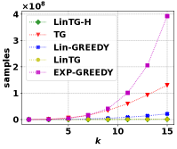
(a) movie60 $\kappa$

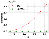
(b) movie5000 $\kappa$

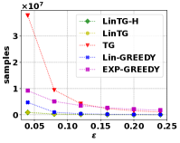
(c) movie60 $\epsilon$

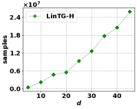
(d) movie500 d

Figure 1: The experimental results of running the algorithms on instances of movie recommendation on the subsets of MovieLens 25M dataset with $n=60$, $d=5$ (”movie60”) and $n=5000$, $d=30$ (”movie5000”), and different datasets with different values of $d$.

Appendix A Appendix for Section 3

In this portion of the appendix, we present missing details and proofs from Section 3 in the main paper. We first present Lemma 1, which guarantees that for any standard greedy-based algorithm which satisfies that the element added at each round has the highest marginal gain within an $\epsilon/\kappa$-additive error, then the ultimate solution set satisfies that $f(S)\geq(1-e^{-1})f(OPT)-\epsilon$. Then we propose and analyze the static allocation strategy LBSS in Section A.1. The pseudocode of LBSS is presented in Algorithm 3 in Section A.1. Finally, we present the missing proofs and details about the theoretical guarantee of LG from Section 3 in Section A.2. Lemma 1 is given as follows.

Lemma 1.

For any standard greedy-based algorithm proposed for our problem, if with probability at least $1-\delta$, the element $a$ added to the solution set $S$ at each round satisfies that $\Delta f(S,a)\geq\max_{s\in U}\Delta f(S,s)-\epsilon/\kappa$, then it follows that the output solution set $S$ satisfies that with probability at least $1-\delta$

$$f(S)\geq(1-e^{-1})f(OPT)-\epsilon.$$

Proof.

The proof of this lemma is similar to the standard greedy algorithm and can be derived from the proof of ExpGreedy in Singla et al. [2016], so we omit the proof here. ∎

A.1 Warm-up: static allocation strategy

In this section, we present the warm-up algorithm LBSS, which combines the standard greedy algorithm with a subroutine inspired by the static allocation proposed in best-arm identification problem in linear bandit Soare et al. [2014]. The strategy is static in that the sequence of sampled feature vectors $\textbf{x}_{a_{t}}$ is independent from the sampling results. However, unlike the static allocation algorithm proposed in Soare et al. [2014], which finds the exact optimal solution, here in LBSS, the algorithm finds the element with the highest marginal gain within an $\epsilon/\kappa$ additive error. The theoretical guarantee is stated below. In particular, we first give a description of the static strategy. Next, we provide the detailed statement and proofs of Theorem 4.

The algorithm proceeds in rounds. In each round, the algorithm selects the element with the highest marginal gain by taking noisy samples of the marginal gains of adding new elements to the current solution set. For notation simplicity, in the following part, we use $\textbf{F}_{x}$ to denote the marginal gain of adding element $x$ to the solution set in the current round $S$. i.e., $\textbf{F}_{x}=\Delta\textbf{F}(S,x)$. The sampled element is chosen in a greedy manner to make $\max_{x,x^{\prime}\in U}||\textbf{F}_{x}-\textbf{F}_{x^{\prime}}||_{\textbf{A}_{t}^{-1}}$ to decrease as fast as possible. It is worthy to note that in LBSS, the update of parameters $\hat{\textbf{w}}_{t}$ is calculated based on the least-square estimator. Therefore, $\textbf{A}_{t+1}=\textbf{A}_{t}+\textbf{x}_{a_{t}}\textbf{x}_{a_{t}}^{T}$, $\textbf{b}_{t+1}=\textbf{b}_{t}+r_{t}\textbf{x}_{a_{t}}$, and that $\hat{\textbf{w}}_{t+1}=\textbf{A}^{-1}_{t+1}\textbf{b}_{t+1}$. The parameter $D_{t}$ is defined as $D_{t}=R\sqrt{2\log(\frac{\pi^{2}t^{2}\kappa n^{2}}{3\delta})}$.

Algorithm 3 Linear Bandit with Static Strategy (LBSS)

1:  Input: $\delta,\epsilon$

2:  Output: solution set $S\subseteq U$

3:  $S\leftarrow\emptyset$

4:  $\textbf{A}\leftarrow\textbf{0}_{d\times d}$, $\textbf{b}\leftarrow\textbf{0}_{d}$

5:  for $l=1,...,\kappa$ do

6:     $t\leftarrow 1$

7:     Define $\textbf{F}_{x}=\Delta\textbf{F}(S,x)$

8:     while  true do

9:        $x_{t}=\arg\min_{x\in U}\max_{x^{\prime},x^{\prime\prime}\in U}(\textbf{F}_{x^{\prime}}-\textbf{F}_{x^{\prime\prime}})^{T}(\textbf{A}_{t}+\textbf{F}_{x}\textbf{F}_{x}^{T})^{-1}(\textbf{F}_{x^{\prime}}-\textbf{F}_{x^{\prime\prime}})$

10:        Obtain the reward $r_{t}$ of sampling $\textbf{F}_{x_{t}}$

11:         Update $\textbf{A}_{t+1}=\textbf{A}_{t}+\textbf{F}_{x_{t}}\textbf{F}_{x_{t}}^{T}$, $\textbf{b}_{t+1}=\textbf{b}_{t}+r_{t}\textbf{F}_{x_{t}}$

12:        Update $\hat{\textbf{w}}_{t+1}=\textbf{A}^{-1}_{t+1}\textbf{b}_{t+1}$

13:        if  $\exists x\in U$, $\forall x^{\prime}\in U$, $D_{t}||\textbf{F}_{x}-\textbf{F}_{x^{\prime}}||_{\textbf{A}_{t}^{-1}}\leq(\textbf{F}_{x}-\textbf{F}_{x^{\prime}})^{T}\hat{\textbf{w}}_{t}+\epsilon$ then

14:           return $x$

15:        end if

16:        $t\leftarrow t+1$

17:     end while

18:  end for

A.1.1 proof of Theorem 4

We now present the missing theoretical proofs for Theorem 4, where we provide bounds on the expectation of the reward of the output element and the sample complexity of LBSS in Algorithm 3.

Theorem 4.

With probability at least $1-\delta$, the following statements hold:

1. The exact function value of the output solution set $S$ satisfies that $f(S)\geq(1-e^{-1})f(OPT)-\epsilon.$ Here $OPT$ is an optimal solution to the SM problem;

2. During each round in LBSS, the number of samples required is upper bounded by

   $$t\leq\max\{\frac{256R^{2}d}{\max\{\Delta_{\min}^{2},\epsilon^{2}/\kappa^{2}\}}\log(\frac{256R^{2}d\pi n}{\max\{\Delta_{\min}^{2},\epsilon^{2}/\kappa^{2}\}}\sqrt{\frac{\kappa}{3\delta}}),\frac{d+d^{2}+2}{2}\}$$

   where $\Delta_{\min}=\min_{\{x^{\prime}\in[n],x^{\prime}\neq x^{*}\}}\textbf{F}_{x^{*}}^{T}\textbf{w}-\textbf{F}_{x^{\prime}}^{T}\textbf{w}$ and $x^{*}=\arg\max_{x\in[n]}\textbf{F}_{x}^{T}\textbf{w}$.

From Lemma 1, we can see that the theorem can be proved immediately by Lemma 2, which is presented below.

Lemma 2.

With probability at least $1-\delta$, in each round of the Algorithm 3, the selected element $x$ satisfies

$$\textbf{F}^{T}_{x}\textbf{w}\geq\textbf{F}^{T}_{x^{*}}\textbf{w}-\epsilon/\kappa.$$ (1)

Besides, the number of samples required by each round is upper bounded by

$$t\leq\max\{\frac{256R^{2}d}{\max\{\Delta_{\min}^{2},\epsilon^{2}/\kappa^{2}\}}\log(\frac{256R^{2}d\pi n}{\max\{\Delta_{\min}^{2},\epsilon^{2}/\kappa^{2}\}}\sqrt{\frac{\kappa}{3\delta}}),\frac{d+d^{2}+2}{2}\}$$

where $\Delta_{\min}=\min_{\{x^{\prime}\in[n],x^{\prime}\neq x^{*}\}}\textbf{F}_{x^{*}}^{T}\textbf{w}-\textbf{F}_{x^{\prime}}^{T}\textbf{w}$, and $x^{*}=\arg\max_{x^{\prime}\in[n]}\textbf{F}_{x^{\prime}}^{T}\textbf{w}$.

Next, we present the proof of Lemma 2.

Proof.

Our argument to prove Lemma 2 follows a similar approach as Soare et al. [2014]. First, we provide proof of (1) on the expectation of the reward of the returned element. Notice that by Proposition 5, and by applying a union bound over all $\kappa$ rounds, with probability at least $1-\delta$, we have that for each round $l$, and for any $x,x^{\prime}\in U$,

$$|(\textbf{F}_{x^{\prime}}-\textbf{F}_{x})^{T}(\textbf{w}-\hat{\textbf{w}}_{t})|\leq||\textbf{F}_{x^{\prime}}-\textbf{F}_{x}||_{\textbf{A}_{t}^{-1}}D_{t}.$$ (2)

From the stopping condition of the algorithm, we know that when the algorithm stops, there exists an element x such that $\forall\textbf{x}^{\prime}\in U$

$$D_{t}||\textbf{F}_{x}-\textbf{F}_{x^{\prime}}||_{\textbf{A}_{t}^{-1}}\leq(\textbf{F}_{x}-\textbf{F}_{x^{\prime}})^{T}\hat{\textbf{w}}_{t}+\epsilon/\kappa.$$

Thus

$$(\textbf{F}_{x}-\textbf{F}_{x^{\prime}})^{T}\textbf{w} =(\textbf{F}_{x}-\textbf{F}_{x^{\prime}})^{T}(\textbf{w}-\hat{\textbf{w}}_{t})+(\textbf{F}_{x}-\textbf{F}_{x^{\prime}})^{T}\hat{\textbf{w}}_{t}$$

$$\geq-D_{t}||\textbf{F}_{x}-\textbf{F}_{x^{\prime}}||_{\textbf{A}_{t}^{-1}}+D_{t}||\textbf{F}_{x}-\textbf{F}_{x^{\prime}}||_{\textbf{A}_{t}^{-1}}-\epsilon/\kappa\geq-\epsilon/\kappa.$$

Since the above inequality holds for any element $\textbf{x}^{\prime}\in U$, we can conclude the proof. In the following part, we prove the sample complexity for this algorithm. By the stopping condition in LBSS in Algorithm 3, we have that during the execution of the algorithm LBSS, for any element $x$, there exists at least one element $x^{\prime}$ such that

$$D_{t}||\textbf{F}_{x}-\textbf{F}_{x^{\prime}}||_{\textbf{A}_{t}^{-1}}\geq(\textbf{F}_{x}-\textbf{F}_{x^{\prime}})^{T}\hat{\textbf{w}}_{t}+\epsilon/\kappa.$$

Therefore, combining the above inequality with (2), it follows that

$$(\textbf{F}_{x}-\textbf{F}_{x^{\prime}})^{T}\textbf{w} =(\textbf{F}_{x}-\textbf{F}_{x^{\prime}})^{T}(\textbf{w}-\hat{\textbf{w}}_{t})+(\textbf{F}_{x}-\textbf{F}_{x^{\prime}})^{T}\hat{\textbf{w}}_{t}$$

$$\leq 2D_{t}||\textbf{F}_{x}-\textbf{F}_{x^{\prime}}||_{\textbf{A}_{t}^{-1}}-\epsilon/\kappa.$$

Since the above result holds for any x, we can set x to be the optimal solution $\textbf{x}^{*}$, then we would have that

$$(\textbf{F}_{x^{*}}-\textbf{F}_{x^{\prime}})^{T}\textbf{w}\leq 2D_{t}||\textbf{F}_{x^{*}}-\textbf{F}_{x^{\prime}}||_{\textbf{A}_{t}^{-1}}-\epsilon/\kappa$$

for some $x^{\prime}$. Therefore,

$$\Delta_{\min}\leq 2D_{t}||\textbf{F}_{x^{*}}-\textbf{F}_{x^{\prime}}||_{\textbf{A}_{t}^{-1}}-\epsilon/\kappa\leq 2D_{t}\max_{x,x^{\prime}\in U}||\textbf{F}_{x}-\textbf{F}_{x^{\prime}}||_{\textbf{A}_{t}^{-1}}-\epsilon/\kappa$$ (3)

where $\Delta_{\min}=\min_{\{x^{\prime}\in[n],x^{\prime}\neq a^{*}\}}\textbf{F}_{x^{*}}^{T}\textbf{w}-\textbf{F}_{x^{\prime}}^{T}\textbf{w}$. Notice that by Lemma 7 and the efficient rounding procedure in Soare et al. [2014], it follows that

$$\max_{x,x^{\prime}\in U}||\textbf{F}_{x}-\textbf{F}_{x^{\prime}}||_{\textbf{A}_{t}^{-1}}\leq 2\sqrt{\frac{(1+\frac{d+d^{2}+2}{2t})d}{t}}.$$

Combine this inequality with (3), we would get

$$4D_{t}\sqrt{\frac{(1+\frac{d+d^{2}+2}{2t})d}{t}}\geq\Delta_{\min}+\epsilon/\kappa.$$

It follows that

$$t\leq\frac{16(1+\frac{d+d^{2}+2}{2t})dD_{t}^{2}}{(\Delta_{\min}+\epsilon/\kappa)^{2}}\leq\frac{16(1+\frac{d+d^{2}+2}{2t})dD_{t}^{2}}{\max\{\Delta_{\min}^{2},\epsilon^{2}/\kappa^{2}\}}$$

We then have that

$$t\leq\max\{\frac{32dD_{t}^{2}}{\max\{\Delta_{\min}^{2},\epsilon^{2}/\kappa^{2}\}},\frac{d+d^{2}+2}{2}\}.$$

From the definition of $D_{t}$, we can get that

$$t\leq\max\{\frac{64R^{2}d\log(\frac{n^{2}t^{2}\pi^{2}}{3\delta})}{\max\{\Delta_{\min}^{2},\epsilon^{2}/\kappa^{2}\}},\frac{d+d^{2}+2}{2}\}.$$

From Lemma 14, we conclude that

$$t\leq\max\{\frac{256R^{2}d}{\max\{\Delta_{\min}^{2},\epsilon^{2}/\kappa^{2}\}}\log(\frac{256R^{2}d\pi n}{\max\{\Delta_{\min}^{2},\epsilon^{2}/\kappa^{2}\}}\sqrt{\frac{\kappa}{3\delta}}),\frac{d+d^{2}+2}{2}\}.$$

∎

A.2 Additional Content to Section 3

In this appendix, we present the missing content in Section 3. First, we provide a detailed discussion on the sampling allocation ratio $p^{*}$ used in LG in Section A.2.1. Next, we delve into the proof of Theorem 2, which provides the theoretical guarantee concerning the algorithm LG.

A.2.1 Discussion on the sample allocation ratio

In our algorithm LG, we use the allocation ratio $p^{*}(l^{\prime},a|l,i,j)$. $p^{*}(l^{\prime},a|l,i,j)$ is the asymptotic-optimal ratio of sampling $\Delta\textbf{F}(S_{l^{\prime}},a)$, which is the marginal gain of adding element $a$ to set $S_{l^{\prime}}$ for decreasing the confidence interval $||\Delta\textbf{F}(S,i)-\Delta\textbf{F}(S,j)||_{\textbf{A}_{t}^{-1}}$ when the number of samples goes to infinity at the round $l$. By Lemma 13, it satisfies that

$$p^{*}(l^{\prime},a|l,i,j)=\frac{|w^{*}_{l^{\prime},a}(i,j)|}{\sum_{l^{\prime\prime}=1}^{l}\sum_{a^{\prime}=1}^{n}|w^{*}_{l^{\prime\prime},a^{\prime}}(i,j)|},$$ (4)

where $\{w^{*}_{l^{\prime},a}(i,j)\}_{a\in[n]}$ is the optimal solution of the linear program in (5) below

$$\arg\min_{\{w_{l^{\prime},a}(i,j)\}}\sum_{l^{\prime}=1}^{l}\sum_{a=1}^{n}|w_{l^{\prime},a}(i,j)|\qquad s.t.\qquad\Delta\textbf{F}(S,i)-\Delta\textbf{F}(S,j)=\sum_{l^{\prime}=1}^{l}\sum_{a=1}^{n}w_{l^{\prime},a}(i,j)\Delta\textbf{F}(S_{l^{\prime}},a).$$ (5)

Besides, as is illustrated in Section 3 and in the proof of Theorem 2 in Section A.2.2, if we replace the asymptotic allocation ratio $p^{*}(l^{\prime},a|l,i,j)$ with any allocation policy $p(l^{\prime},a|l,i,j)$, we can still obtain a theoretical guarantee on the upper bound of the sample complexity for our algorithm LG. In particular, by setting the allocation ratio to $p(l^{\prime},a|l,i,j)=0.5$ for $l^{\prime}=l$ and $a=i$ or $j$, and $p(l^{\prime},a|l,i,j)=0$ otherwise, the allocation strategy in LG is similar to that used in the CLUCB algorithm in Chen et al. [2014]. Both these two algorithms sample the direction between $\Delta\textbf{F}(S,i)$ and $\Delta\textbf{F}(S,j)$ to decrease $||\Delta\textbf{F}(S,i)-\Delta\textbf{F}(S,j)||_{\textbf{A}_{t}^{-1}}$. Although this allocation ratio is not asymptotically optimal and follows a similar principle to the CLUCB algorithm, there are notable differences: (i) Our algorithm LG leverages the linear structure, and the concentration inequality used is derived from the linear bandit literature. (ii). The linear submodular bandit algorithm allows us to exploit sampling results from past greedy rounds while in the CLUCB algorithm developed for the general bandit setting, we are not allowed to do that. In our experiments, we also adopt this allocation ratio.

A.2.2 Proof of Theorem 2

In this section, we prove Theorem 2, which guarantees the sample complexity and approximation ratio of LG. From Lemma 1, we can see that proving Theorem 2 is equivalent to proving the following result.

Lemma 3.

With probability at least $1-\delta$, in each round of the LG in Algorithm 1, the selected element $a$ satisfies

$$\Delta\textbf{F}^{T}(S,a)\textbf{w}\geq\max_{x\in[n]}\Delta\textbf{F}^{T}(S,x))\textbf{w}-\epsilon/\kappa$$

Besides, assume $\lambda\leq\frac{2R^{2}}{S^{2}}\log\frac{1}{\delta}$, then during the round $l$, the total number of samples $\tau$ satisfies

$$\tau \leq\sum_{l^{\prime}\in[l],a\in[n]}\max\{4H^{(l)}_{l^{\prime},a}R^{2}(2\log\frac{1}{\delta}+d\log M^{(l)})+1-N_{l^{\prime},a}^{(l)},0\},$$

where $M^{(l)}=\frac{16H_{\epsilon}^{(l)}R^{2}L^{2}}{\lambda}\log(\frac{1}{\delta})+\frac{32(H_{\epsilon}^{(l)})^{2}R^{4}L^{4}}{\lambda^{2}}+\frac{2(N^{(l)}+nl)L^{2}}{\lambda d}+2$. Here $H_{l^{\prime},a}^{(l)}=\max_{i,j\in[n]}\frac{p^{*}(l^{\prime},a|l,i,j)\rho_{i,j}^{l}}{\max\{\epsilon/\kappa,\frac{\Delta_{l,i}\vee\Delta_{l,j}+\epsilon/\kappa}{3}\}^{2}}$ and $H_{\epsilon}^{(l)}=\sum_{l^{\prime}\in[l],a\in[n]}H_{l^{\prime},a}^{(l)}$, where $\rho_{i,j}^{l}$ is the optimal value of (5).

Proof.

Throughout the proof, we assume the clean event $\mathcal{E}$ occurs. The event $\mathcal{E}$ is defined as

$$\mathcal{E}=\{\forall t>0,\forall i,j\in[n],|(\Delta\textbf{F}(S,i)-\Delta\textbf{F}(S,j))^{T}(\hat{\textbf{w}}-\textbf{w})|\leq\beta_{t}(i,j)\},$$

where the confidence interval $\beta_{t}(i,j)=C_{t}||\Delta\textbf{F}(S,i)-\Delta\textbf{F}(S,j)||_{\textbf{A}_{t}}^{-1}$ and that $C_{t}=R\sqrt{2\log\frac{\det(\textbf{A}_{t})^{\frac{1}{2}}\det(\lambda I)^{-\frac{1}{2}}}{\delta}}+\lambda^{\frac{1}{2}}S$. Then by Proposition 1, and the fact that for all $i$, $\Delta\textbf{F}(S,i)$ only depends on the past samples of marginal gains, we have the following lemma.

Lemma 4.

With probability at least $1-\delta$, event $\mathcal{E}$ holds.

First of all, we prove the result on the correctness of the output element $i_{t}$. Let us denote that $a^{*}=\arg\max_{a\in[n]}\Delta\textbf{F}(S,a)^{T}\textbf{w}$, and that $\epsilon^{\prime}=\epsilon/\kappa$. By the stopping condition in LG, we have that

$$B(t)=(\Delta\textbf{F}(S,j_{t})-\Delta\textbf{F}(S,i_{t}))^{T}\hat{\textbf{w}}+\beta_{t}(i_{t},j_{t})\leq\epsilon^{\prime}.$$

By the selection strategy of $j_{t}$, we have that $B(t)\geq(\Delta\textbf{F}(S,a^{*})-\Delta\textbf{F}(S,i_{t}))^{T}\hat{\textbf{w}}+\beta_{t}(a^{*},i_{t})^{T}$. Therefore, by Lemma 4, we have that

$$(\Delta\textbf{F}(S,a^{*})-\Delta\textbf{F}(S,i_{t}))^{T}\textbf{w}\leq(\Delta\textbf{F}(S,a^{*})-\Delta\textbf{F}(S,i_{t}))^{T}\hat{\textbf{w}}+\beta_{t}(a^{*},i_{t})\leq\epsilon^{\prime}.$$

Next, we prove the theoretical guarantee of the sample complexity. Let us denote $\Delta_{l,i}$ to be the gap between element $i$ and the element with the highest marginal gain at round $l$, i.e., $\Delta_{l,i}=\max_{x\in[n]}\Delta\textbf{F}(S_{l},x)^{T}\textbf{w}-\Delta\textbf{F}(S_{l},i)^{T}\textbf{w}$. At the round $l$, we have that the solution set $S=S_{l}$. For notation simplicity, we denote $\Delta_{i}=\max_{x\in[n]}\Delta\textbf{F}(S,x)^{T}\textbf{w}-\Delta\textbf{F}(S,i)^{T}\textbf{w}$. From Lemma 4 in the appendix of Xu et al. [2018], we have

Lemma 5.

Under event $\mathcal{E}$, throughout the execution of LG, $B(t)$ can be bounded as

$$B(t)\leq\min(0,-(\Delta_{i_{t}}\vee\Delta_{j_{t}})+2\beta_{t}(i_{t},j_{t}))+\beta_{t}(i_{t},j_{t}).$$

The proof is the same as in Xu et al. [2018], so we omit the proof here. First of all, we derive the bound on the total number of samples for each element $a$ from the sampling set $\mathcal{X}$. Then by Lemma 5 and that $B(t)\geq\epsilon^{\prime}$ we have that

$$\beta_{t}(i_{t},j_{t})\geq\max\{\epsilon^{\prime},\frac{\Delta_{i_{t}}\vee\Delta_{j_{t}}+\epsilon^{\prime}}{3}\}.$$

By the definition of the confidence interval $\beta_{t}(i_{t},j_{t})$, we have that

$$||\Delta\textbf{F}(S,i_{t})-\Delta\textbf{F}(S,j_{t})||_{\textbf{A}_{t}^{-1}}\geq\frac{\max\{\epsilon^{\prime},\frac{\Delta_{i_{t}}\vee\Delta_{j_{t}}+\epsilon^{\prime}}{3}\}}{C_{t}}.$$

Since we have

$$||\Delta\textbf{F}(S,i_{t})-\Delta\textbf{F}(S,j_{t})||_{\textbf{A}_{t}^{-1}}$$ (6)

$$= \sqrt{(\Delta\textbf{F}(S,i_{t})-\Delta\textbf{F}(S,j_{t}))^{T}\textbf{A}_{t}^{-1}(\Delta\textbf{F}(S,i_{t})-\Delta\textbf{F}(S,j_{t}))}$$

$$= \sqrt{(\Delta\textbf{F}(S,i_{t})-\Delta\textbf{F}(S,j_{t}))^{T}(\sum_{l^{\prime\prime}\in[l]}\sum_{a^{\prime}\in[n]}T_{l^{\prime\prime},a^{\prime}}(t)\Delta\textbf{F}(S_{l^{\prime\prime}},a^{\prime})\Delta\textbf{F}(S_{l^{\prime\prime}},a^{\prime})^{T}))^{-1}(\Delta\textbf{F}(S,i_{t})-\Delta\textbf{F}(S,j_{t}))}.$$ (7)

Suppose the marginal gain of adding an element $a$ to subset $S_{l^{\prime}}$ is sampled at time $t$, from the element selection strategy, we have that for any other past marginal gain vectors, it follows that for any $l^{\prime\prime}\in[l]$ and $a^{\prime}\in[n]$,

$$\frac{T_{l^{\prime},a}(t)}{p^{*}(l^{\prime},a|l,i_{t},j_{t})}\leq\frac{T_{l^{\prime\prime},a^{\prime}}(t)}{p^{*}(l^{\prime\prime},a^{\prime}|l,i_{t},j_{t})}.$$

Combine (6) with the above inequality, it follows that

$$||\Delta\textbf{F}(S,i_{t})-\Delta\textbf{F}(S,j_{t})||_{\textbf{A}_{t}^{-1}}\leq\sqrt{\frac{p^{*}(l^{\prime},a|l,i_{t},j_{t})}{T_{l^{\prime},a}(t)}}||\Delta\textbf{F}(S,i_{t})-\Delta\textbf{F}(S,j_{t})||_{\Lambda_{i_{t},j_{t}}^{-1}}$$

where we define

$$\Lambda_{i,j}=\sum_{l^{\prime\prime}\in[l]}\sum_{a^{\prime}\in[n]}p^{*}(l^{\prime\prime},a^{\prime}|l,i,j)\Delta\textbf{F}(S_{l^{\prime\prime}},a^{\prime})\Delta\textbf{F}^{T}(S_{l^{\prime\prime}},a^{\prime}).$$ (8)

Therefore, we have

$$T_{l^{\prime},a}(t)\leq\frac{p^{*}(l^{\prime},a|l,i_{t},j_{t})||\Delta\textbf{F}(S,i_{t})-\Delta\textbf{F}(S,j_{t})||^{2}_{\Lambda_{i_{t},j_{t}}^{-1}}C_{t}^{2}}{\max\{\epsilon^{\prime},\frac{\Delta_{i_{t}}\vee\Delta_{j_{t}}+\epsilon^{\prime}}{3}\}^{2}}$$

$$\leq\max_{i,j\in[n]}\frac{p^{*}(l^{\prime},a|l,i,j)||\Delta\textbf{F}(S,i)-\Delta\textbf{F}(S,j)||^{2}_{\Lambda_{i,j}^{-1}}C_{t}^{2}}{\max\{\epsilon^{\prime},\frac{\Delta_{i}\vee\Delta_{j}+\epsilon^{\prime}}{3}\}^{2}}$$

Let $\tau^{\prime}$ denote the total number of samples in round $l$, encompassing both the offline dataset and the samples acquired during the execution of LG. Consequently, upon termination of the algorithm, the cumulative number of samples associated with element $a$ is bounded by:

$$T_{l^{\prime},a}(\tau^{\prime})\leq\max_{i,j\in[n]}\frac{p^{*}(l^{\prime},a|l,i,j)||\Delta\textbf{F}(S,i)-\Delta\textbf{F}(S,j)||^{2}_{\Lambda_{i,j}^{-1}}C_{\tau^{\prime}}^{2}}{\max\{\epsilon^{\prime},\frac{\Delta_{i}\vee\Delta_{j}+\epsilon^{\prime}}{3}\}^{2}}+1.$$ (9)

Notice that we can reuse $N_{l^{\prime},a}^{(l)}$ samples from the past rounds, therefore, the total number of samples of element $a$ in round $l$ in LG is bounded by

$$\max\{T_{l^{\prime},a}(\tau^{\prime})-N_{l^{\prime},a}^{(l)},0\}.$$

The total number of samples for all the elements in round $l$ during the execution of LG is bounded by

$$\tau\leq\sum_{l^{\prime}\in[l]}\sum_{a\in[n]}\max\{T_{l^{\prime},a}(\tau^{\prime})-N_{l^{\prime},a}^{(l)},0\}.$$

Combine this inequality with (9), we get that

$$\tau \leq\sum_{l^{\prime}\in[l]}\sum_{a\in[n]}\max\{\max_{i,j\in[n]}\frac{p^{*}(l^{\prime},a|l,i,j)||\Delta\textbf{F}(S,i)-\Delta\textbf{F}(S,j)||^{2}_{\Lambda_{i,j}^{-1}}C_{\tau^{\prime}}^{2}}{\max\{\epsilon^{\prime},\frac{\Delta_{i}\vee\Delta_{j}+\epsilon^{\prime}}{3}\}^{2}}+1-N_{l^{\prime},a}^{(l)},0\}$$

$$\leq\sum_{l^{\prime}\in[l]}\sum_{a\in[n]}\max\{\max_{i,j\in[n]}\frac{p^{*}(l^{\prime},a|l,i,j)||\Delta\textbf{F}(S,i)-\Delta\textbf{F}(S,j)||^{2}_{\Lambda_{i,j}^{-1}}C_{\tau+N^{(l)}}^{2}}{\max\{\epsilon^{\prime},\frac{\Delta_{i}\vee\Delta_{j}+\epsilon^{\prime}}{3}\}^{2}}+1-N_{l^{\prime},a}^{(l)},0\}$$

where $N^{(l)}=\sum_{l^{\prime}\in[l]}\sum_{a\in[n]}N_{l^{\prime},a}^{(l)}$ is the total number of samples in the offline dataset.

From Lemma 13 and the discussion given in Appendix B in Xu et al. [2018], we have that the allocation ratio $p^{*}$ is the optimal solution of the optimization problem as defined in (4) and (5), then it follows that

$$||\Delta\textbf{F}(S,i)-\Delta\textbf{F}(S,j)||^{2}_{\Lambda_{i,j}^{-1}}\leq\rho_{i,j}^{l}.$$

where $\rho_{i,j}^{l}$ is the optimal value of (5) in the round $l$.

Let us denote $H_{l^{\prime},a}^{(l)}=\max_{i,j\in[n]}\frac{p^{*}(l^{\prime},a|l,i,j)\rho_{i,j}^{l}}{\max\{\epsilon/\kappa,\frac{\Delta_{l,i}\vee\Delta_{l,j}+\epsilon/\kappa}{3}\}^{2}}$ and $H_{\epsilon}^{(l)}=\sum_{l^{\prime}\in[l],a\in[n]}H_{l^{\prime},a}^{(l)}$. Then the inequality above is

$$\tau \leq\sum_{l^{\prime}\in[l]}\sum_{a\in[n]}\max\{H_{l^{\prime},a}^{(l)}C_{\tau+N}^{2}+1-N_{l^{\prime},a}^{(l)},0\}.$$ (10)

It then follows that

$$\tau \leq H_{\epsilon}^{(l)}C_{\tau+N}^{2}+nl.$$ (11)

By definition, we have that

$$C_{t}=R\sqrt{2\log\frac{\det(\textbf{A}_{t})^{\frac{1}{2}}\det(\lambda I)^{-\frac{1}{2}}}{\delta}}+\lambda^{\frac{1}{2}}S.$$

By Lemma 12, we can get that

$$C_{t}\leq R\sqrt{2\log\frac{1}{\delta}+d\log(1+\frac{tL^{2}}{\lambda d})}+\lambda^{\frac{1}{2}}S.$$

Since $\lambda\leq\frac{2R^{2}}{S^{2}}\log\frac{1}{\delta}$, it follows that

$$C_{t}\leq 2R\sqrt{2\log\frac{1}{\delta}+d\log(1+\frac{tL^{2}}{\lambda d})}.$$ (12)

Combine (11) with (12), we can get

$$\tau\leq 4H_{\epsilon}^{(l)}R^{2}\big{(}2\log\frac{1}{\delta}+d\log(1+\frac{(\tau+N^{(l)})L^{2}}{\lambda d})\big{)}+nl$$

It then follows that

$$\frac{(\tau+N^{(l)})L^{2}}{\lambda d}+1\leq\frac{4H_{\epsilon}^{(l)}R^{2}L^{2}}{\lambda d}\big{(}2\log\frac{1}{\delta}+d\log(1+\frac{(\tau+N^{(l)})L^{2}}{\lambda d})\big{)}+\frac{(N^{(l)}+nl)L^{2}}{\lambda d}+1$$

By Lemma 15, we have that

$$\frac{(\tau+N^{(l)})L^{2}}{\lambda d}+1 \leq\frac{16H_{\epsilon}^{(l)}R^{2}L^{2}}{\lambda d}\log\frac{1}{\delta}+\frac{8H_{\epsilon}^{(l)}R^{2}L^{2}}{\lambda}\log(\frac{4H_{\epsilon}R^{2}L^{2}}{\lambda})+\frac{2(N^{(l)}+nl)L^{2}}{\lambda d}+2$$

$$\leq\frac{16H_{\epsilon}^{(l)}R^{2}L^{2}}{\lambda}\log\frac{1}{\delta}+\frac{32(H_{\epsilon}^{(l)})^{2}R^{4}L^{4}}{\lambda^{2}}+\frac{2(N^{(l)}+nl)L^{2}}{\lambda d}+2.$$

Plugging the above inequality into (10), it follows that

$$\tau \leq\sum_{l^{\prime}\in[l]}\sum_{a\in[n]}\max\{4H_{l^{\prime},a}^{(l)}R^{2}(2\log\frac{1}{\delta}+d\log M)+1-N_{l^{\prime},a}^{(l)},0\}.$$

where $M=\frac{16H_{\epsilon}^{(l)}R^{2}L^{2}}{\lambda}\log\frac{1}{\delta}+\frac{32(H_{\epsilon}^{(l))^{2}}R^{4}L^{4}}{\lambda^{2}}+\frac{2(N^{(l)}+nl)L^{2}}{\lambda d}+2.$ ∎

Appendix B Appendix for Section 4

In this section, we present the proofs of theoretical results from Section 4. First, in Section B.1, we present and prove the Lemma 6 concerning the theoretical guarantee on the value of the evaluated marginal gain and sample complexity of LinTG. Next, we apply the theoretical results of Lemma 6 and prove the final theoretical guarantee for the linear threshold greedy algorithm LinTG in Algorithm 2.

B.1 Proof of Lemma 6

We prove the theoretical guarantee about evaluation of each marginal gain in LinTG. First of all, we present the detailed statements of Lemma 6. First, we notice that by Lemma 13, we have that $p^{*}$ at the $m$-th evaluation of marginal gain can be calculated by

$$p^{*}_{i}=\frac{|w^{*}_{i}|}{\sum_{i\in[m]}|w^{*}_{i}|}$$ (13)

where $w_{i}^{*}$ is the optimal solution to the linear programming problem below.

$$\arg\min_{\{w_{i}\}}\sum_{i\in[m]}|w_{i}|\qquad s.t.\qquad\Delta\textbf{F}(S_{m},a_{m})=\sum_{i=1}^{m}w_{i}\Delta\textbf{F}(S_{i},a_{i}).$$ (14)

In addition, we denote the optimal value of the above optimization problem as $\rho^{(m)}$. In our experiments, we also consider the allocation ratio of $p_{i}=0$ for $i\neq m$ and $p_{m}=1$, i.e., the algorithm always samples the marginal gain $\Delta f(S_{m},a_{m})$ to determine whether $\Delta f(S_{m},a_{m})$ is approximately above $w$ or not.

Lemma 6.

During the $m$-th evaluation on the marginal gain of adding element $a_{m}$ to $S_{m}$ in LinTG, we have that with probability at least $1-\delta/2$, the following statement holds.

1. Assuming $\lambda\leq\frac{2R^{2}}{S^{2}}\log\frac{2}{\delta}$, then it takes at most

   $$\sum_{i\in[m]}\max\{4H^{(m)}_{i}R^{2}(2\log\frac{2}{\delta}+d\log M^{(m)})+1-N_{i}^{(m)},0\}$$

   samples to evaluate the $m$-th marginal gain, where $M^{(m)}=\frac{16H_{\epsilon}^{(m)}R^{2}L^{2}}{\lambda}\log\frac{2}{\delta}+\frac{32(H_{\epsilon}^{(m)})^{2}R^{4}L^{4}}{\lambda^{2}}+\frac{2(N^{(m)}+m)L^{2}}{\lambda d}+2$. Here $H_{i}^{(m)}=\frac{p^{*}_{i}\rho^{(m)}}{\max\{\frac{\epsilon/\kappa+|w-\Delta\textbf{F}(S,a)^{T}\textbf{w}|}{2},\epsilon/\kappa\}^{2}}$ and $H_{\epsilon}^{(m)}=\sum_{i\in[m]}H_{i}^{(m)}$. $p^{*}_{i}$ is the fraction of samples allocated to sample $\Delta\textbf{F}(S_{i},a_{i})$ and therefore $\sum_{i\in[m]}p^{*}_{i}=1$. $\rho^{(m)}$ is the optimal value of

   $$\arg\min_{\{w_{i}\}}\sum_{i\in[m]}|w_{i}|\qquad s.t.\qquad\Delta\textbf{F}(S_{m},a_{m})=\sum_{i=1}^{m}w_{i}\Delta\textbf{F}(S_{i},a_{i}).$$ (15)

2. If the element is added to the solution set, then $\Delta\textbf{F}(S_{m},a_{m})^{T}\textbf{w}\geq w-\epsilon/\kappa$. Otherwise, $\Delta\textbf{F}(S_{m},a_{m})^{T}\textbf{w}\leq w+\epsilon/\kappa$.

For notation simplicity, throughout the proof, we define $\epsilon^{\prime}=\epsilon/\kappa$. To prove this lemma, We first present the following Lemma 7 and Lemma 8 about our algorithm LinTG. Once these lemmas are proven, we next prove the main result of Lemma 6 using the lemmas. We start by introducing the following ”clean event”.

$$\mathcal{E}=\{|\Delta\textbf{F}(S_{m},a_{m})^{T}(\hat{\textbf{w}}-\textbf{w})|\leq\beta_{t},\forall t\}$$

Here $\beta_{t}$ is the confidence interval and is defined as $\beta_{t}=C_{t}||\Delta\textbf{F}(S_{m},a_{m})||_{\textbf{A}_{t}^{-1}}=(R\sqrt{2\log\frac{2\det(\textbf{A}_{t})^{\frac{1}{2}}\det(\lambda I)^{-\frac{1}{2}}}{\delta}}+\lambda^{\frac{1}{2}}S)||\Delta\textbf{F}(S_{m},a_{m})||_{\textbf{A}_{t}^{-1}}$. From the fact that $\Delta\textbf{F}(S_{m},a_{m})$ only depends on the offline dataset, i.e., the history up to time $t$, we can apply the result in Proposition 1. It follows that $P(\mathcal{E})\geq 1-\frac{\delta}{2}$. Therefore, we have the following lemma.

Lemma 7.

With probability at least $1-\delta/2$, it holds that

$$P(\mathcal{E})\geq 1-\delta.$$

Next, we prove the bound on the confidence interval $\beta_{t}$.

Lemma 8.

Conditioned on the event $\mathcal{E}$, the confidence interval $\beta_{t}$ satisfies that

$$\beta_{t}\geq\max\{\frac{\epsilon^{\prime}+|w-\Delta\textbf{F}(S_{m},a_{m})^{T}\textbf{w}|}{2},\epsilon^{\prime}\}$$

before the evaluation of the marginal gain ends.

Proof.

It is equivalent to prove that when $\beta_{t}\leq\frac{\epsilon^{\prime}+|w-\Delta\textbf{F}(S_{m},a_{m})^{T}\textbf{w}|}{2}$, the evaluation of the marginal gain ends. If $\beta_{t}\leq\frac{\epsilon^{\prime}+w-\Delta\textbf{F}(S_{m},a_{m})^{T}\textbf{w}}{2}$, then we have $\Delta\textbf{F}(S_{m},a_{m})^{T}\textbf{w}\leq w+\epsilon^{\prime}-2\beta_{t}$. From Lemma 4, we have that with probability at least $1-\delta$, it holds that $\Delta\textbf{F}(S_{m},a_{m})^{T}\hat{\textbf{w}}-\Delta\textbf{F}(S_{m},a_{m})^{T}\textbf{w}\leq\beta_{t}$. Therefore,

$$\Delta\textbf{F}(S_{m},a_{m})^{T}\hat{\textbf{w}}+\beta_{t}$$

$$\leq(\Delta\textbf{F}(S_{m},a_{m})^{T}\hat{\textbf{w}}-\Delta\textbf{F}(S_{m},a_{m})^{T}\textbf{w})+\Delta\textbf{F}(S_{m},a_{m})^{T}\textbf{w}+\beta_{t}$$

$$\leq w+\epsilon^{\prime}.$$

Thus the algorithm ends.

Similarly, we consider the case where $\beta_{t}\leq\frac{\epsilon^{\prime}-w+\Delta\textbf{F}(S_{m},a_{m})^{T}\textbf{w}}{2}$. In this case, we have that $\Delta\textbf{F}(S_{m},a_{m})^{T}\textbf{w}\geq 2\beta_{t}+w-\epsilon^{\prime}$. Notice that conditioned on the clean event defined in Lemma 4, we have that $\Delta\textbf{F}(S_{m},a_{m})^{T}\hat{\textbf{w}}-\Delta\textbf{F}(S_{m},a_{m})^{T}\textbf{w}\geq-\beta_{t}$. Then

$$\Delta\textbf{F}(S_{m},a_{m})^{T}\hat{\textbf{w}}-\beta_{t} \geq\Delta\textbf{F}(S_{m},a_{m})^{T}\hat{\textbf{w}}-\Delta\textbf{F}(S_{m},a_{m})^{T}\textbf{w}$$

$$\qquad+\Delta\textbf{F}(S_{m},a_{m})^{T}\textbf{w}-\beta_{t}$$

$$\geq-\beta_{t}+2\beta_{t}$$

$$\qquad+w-\epsilon^{\prime}-\beta_{t}$$

$$=w-\epsilon^{\prime}.$$

Therefore, the algorithm ends. In the case where $\beta_{t}\leq\epsilon^{\prime}$, then $w+\epsilon^{\prime}-\beta_{t}\geq w-\epsilon^{\prime}+\beta_{t}$. Therefore, either we have $\Delta\textbf{F}(S_{m},a_{m})^{T}\hat{\textbf{w}}\geq w+\beta_{t}-\epsilon^{\prime}$ or $\Delta\textbf{F}(S_{m},a_{m})^{T}\hat{\textbf{w}}\leq w-\beta_{t}+\epsilon^{\prime}$. Thus the the evaluation of the $m$-th marginal gain ends. ∎

Now we can prove Lemma 6.

Proof.

First of all, we prove the second result in the Lemma 6. Conditioned on the event $\mathcal{E}$ , we have that if the $a_{m}$ element is added to $S_{m}$, then

$$\Delta\textbf{F}(S_{m},a_{m})^{T}\textbf{w}\geq\Delta\textbf{F}(S_{m},a_{m})^{T}\hat{\textbf{w}}-\beta_{t}\geq w-\epsilon^{\prime}.$$

If the $a_{m}$ element is not added to $S_{m}$, then

$$\Delta\textbf{F}(S_{m},a_{m})^{T}\textbf{w}\leq\Delta\textbf{F}(S_{m},a_{m})^{T}\hat{\textbf{w}}+\beta_{t}\leq w+\epsilon^{\prime}.$$

Next, we prove our first result, which provides the theoretical guarantee of sample complexity. The proof depends on Lemma 8. By Lemma 8, and the definition of $\beta_{t}$, we have that

$$C_{t}||\Delta\textbf{F}(S_{m},a_{m})||_{\textbf{A}_{t}^{-1}}\geq\max\{\frac{\epsilon^{\prime}+|w-\Delta\textbf{F}(S_{m},a_{m})^{T}\textbf{w}|}{2},\epsilon^{\prime}\}.$$

Similar to the proof in Lemma 5, we have that the sampled element $i_{t}$ satisfies

$$||\Delta\textbf{F}(S_{m},a_{m})||_{\textbf{A}_{t}^{-1}}\leq\sqrt{\frac{p_{i_{t}}^{*}}{T_{i_{t}}(t)}}||\Delta\textbf{F}(S_{m},a_{m})||_{\Lambda^{-1}},$$

where $\Lambda=\sum_{i\in[m]}p_{i}^{*}\Delta\textbf{F}(S_{i},a_{i})\Delta\textbf{F}(S_{i},a_{i})^{T}$. Therefore, before the marginal gain of adding $a_{i_{t}}$ to $S_{i_{t}}$ is sampled at time $t$, we have

$$T_{i_{t}}(t)\leq\frac{p_{i_{t}}^{*}||\Delta\textbf{F}(S_{m},a_{m})||^{2}_{\Lambda^{-1}}C_{t}^{2}}{\max\{\frac{\epsilon^{\prime}+|w-\Delta\textbf{F}(S_{m},a_{m})^{T}\textbf{w}|}{2},\epsilon^{\prime}\}^{2}}.$$

For any other marginal gain with index $i$, suppose $\tilde{t}$ is the last time $\Delta\textbf{F}(S_{i},a_{i})$ is sampled, and that $\tau^{\prime}$ is the total number of samples, then

$$T_{i}(\tau^{\prime})=T_{i}(\tilde{t})+1\leq\frac{p_{i}^{*}||\Delta\textbf{F}(S_{m},a_{m})||^{2}_{\Lambda^{-1}}C_{\tau^{\prime}}^{2}}{\max\{\frac{\epsilon^{\prime}+|w-\Delta\textbf{F}(S_{m},a_{m})^{T}\textbf{w}|}{2},\epsilon^{\prime}\}^{2}}+1.$$

Since $T_{i}(\tau^{\prime})$ is the total number of samples to the marginal gain $\Delta\textbf{F}(S_{i},a_{i})$ including the past samples, then the total number of samples of $\Delta\textbf{F}(S_{i},a_{i})$ during the evaluation of $\Delta\textbf{F}(S_{m},a_{m})$ is upper bounded by

$$\max\{\frac{p_{i}^{*}||\Delta\textbf{F}(S_{m},a_{m})||^{2}_{\Lambda^{-1}}C_{\tau^{\prime}}^{2}}{\max\{\frac{\epsilon^{\prime}+|w-\Delta\textbf{F}(S_{m},a_{m})^{T}\textbf{w}|}{2},\epsilon^{\prime}\}^{2}}+1-N_{i}^{(m)},0\}.$$

Summing over all elements, we would get

$$\tau \leq\sum_{i\in[m]}\max\{\frac{p_{i}^{*}||\Delta\textbf{F}(S_{m},a_{m})||^{2}_{\Lambda^{-1}}C_{\tau^{\prime}}^{2}}{\max\{\frac{\epsilon^{\prime}+|w-\Delta\textbf{F}(S_{m},a_{m})^{T}\textbf{w}|}{2},\epsilon^{\prime}\}^{2}}+1-N_{i}^{(m)},0\}$$

$$\leq\sum_{i\in[m]}\max\{\frac{p_{i}^{*}||\Delta\textbf{F}(S_{m},a_{m})||^{2}_{\Lambda^{-1}}C_{\tau+N^{(m)}}^{2}}{\max\{\frac{\epsilon^{\prime}+|w-\Delta\textbf{F}(S_{m},a_{m})^{T}\textbf{w}|}{2},\epsilon^{\prime}\}^{2}}+1-N_{i}^{(m)},0\},$$

where $N^{(m)}$ is the total number of samples in the offline dataset. By Lemma 13, it follows that

$$\tau \leq\sum_{i\in[m]}\max\{\frac{p_{i}^{*}\rho^{(m)}C_{\tau+N^{(m)}}^{2}}{\max\{\frac{\epsilon^{\prime}+|w-\Delta\textbf{F}(S_{m},a_{m})^{T}\textbf{w}|}{2},\epsilon^{\prime}\}^{2}}+1-N_{i}^{(m)},0\},$$

where $\rho^{(m)}$ is the optimal value of the optimization problem in (14). Let us denote $H_{i}^{(m)}=\frac{p_{i}^{*}\rho^{(m)}}{\max\{\frac{\epsilon^{\prime}+|w-\Delta\textbf{F}(S_{m},a_{m})^{T}\textbf{w}|}{2},\epsilon^{\prime}\}^{2}}$ and $H_{\epsilon}^{(m)}=\sum_{i\in[m]}H_{i}^{(m)}=\frac{\rho^{(m)}}{\max\{\frac{\epsilon^{\prime}+|w-\Delta\textbf{F}(S_{m},a_{m})^{T}\textbf{w}|}{2},\epsilon^{\prime}\}^{2}}$. Then the inequality above is

$$\tau \leq\sum_{i\in[m]}\max\{H_{i}^{(m)}C_{\tau+N^{(m)}}^{2}+1-N_{i}^{(m)},0\}.$$ (16)

It then follows that

$$\tau \leq H_{\epsilon}^{(m)}C_{\tau+N^{(m)}}^{2}+m$$ (17)

Similar to the proof of Theorem 3, we have that

$$\tau \leq\sum_{i\in[m]}\max\{4H_{i}^{(m)}R^{2}(2\log\frac{2}{\delta}+d\log M^{(m)})+1-N_{i}^{(m)},0\}.$$

where $M^{(m)}=\frac{16H_{\epsilon}^{(m)}R^{2}L^{2}}{\lambda}\log\frac{2}{\delta}+\frac{32(H_{\epsilon}^{(m)})^{2}R^{4}L^{4}}{\lambda^{2}}+\frac{2(N^{(m)}+m)L^{2}}{\lambda d}+2.$ ∎

B.2 Proof of Theorem 3

In this section, we present the proof of Theorem 3.

Theorem 3. LinTG makes $n\log(\kappa/\alpha)/\alpha$ evaluations of the marginal gains. In addition, with probability at least $1-\delta$, the following statements hold:

1. The function value of the output solution set $S$ satisfies that $f(S)\geq(1-e^{-1}-\alpha)f(OPT)-2\epsilon.$ Here $OPT$ is an optimal solution to the SM problem;

2. Assuming $\lambda\leq\frac{2R^{2}}{S^{2}}\log\frac{2}{\delta}$, the $m$-th evaluation of the marginal gain of adding an element $a$ to $S$ in LinTG takes at most

   $$\sum_{i\in[m]}\max\{4H^{(m)}_{i}R^{2}(2\log\frac{2}{\delta}+d\log M^{(m)})+1-N_{i}^{(m)},0\}$$

   samples, where $M^{(m)}=\frac{16H_{\epsilon}^{(m)}R^{2}L^{2}}{\lambda}\log\frac{2}{\delta}+\frac{32(H_{\epsilon}^{(m)})^{2}R^{4}L^{4}}{\lambda^{2}}+\frac{2(N^{(m)}+m)L^{2}}{\lambda d}+2$. Here $H_{i}^{(m)}=\frac{p^{*}_{i}\rho^{(m)}}{\max\{\frac{\epsilon/\kappa+|w-\Delta\textbf{F}(S_{m},a_{m})^{T}\textbf{w}|}{2},\epsilon/\kappa\}^{2}}$ and $H_{\epsilon}^{(m)}=\sum_{i\in[m]}H_{i}^{(m)}$. $p^{*}_{i}$ is the fraction of samples allocated to sample $\Delta\textbf{F}(S_{i},a_{i})$. $N^{(m)}$ is the total number of samples before the $m$-th evaluation of marginal gains. $N^{(m)}_{i}$ is the number of samples to the marginal gain $\Delta f(S_{i},a_{i})$ before the $m$-th evaluation of marginal gains.

The second result can be obtained by applying the result in Lemma 6. To prove the first result, we first present a series of needed lemmas. In order for the guarantees of Theorem 3 to hold, two random events must occur during LG. The first event is that the estimate of the max singleton value of $f$ on Line 5 in LG is an $\epsilon$-approximation of its true value. More formally, we have the following lemma.

Lemma 9.

With probability at least $1-\delta/3$, we have $\max_{s\in U}f(s)-\epsilon\leq g\leq\max_{s\in U}f(s)+\epsilon$.

Proof.

For a fix $s\in U$, by Hoeffding’s inequality we would have that

$$P(|\hat{f}(s)-f(s)|\geq\epsilon)\leq\frac{\delta}{3n}.$$ (18)

Taking a union bound over all elements we would have that

$$P(\exists s\in U,s.t.|\hat{f}(s)-f(s)|\geq\epsilon)\leq\frac{\delta}{3}.$$

Then with probability at least $1-\frac{\delta}{3}$, $|\hat{f}(s)-f(s)|\leq\epsilon$ for all $s\in U$. It then follows that $\forall s\in U$, $f(s)-\epsilon\leq\hat{f}(s)\leq f(s)+\epsilon$. Therefore

$$\max_{s\in U}(f(s)-\epsilon)\leq\max_{s\in U}\hat{f}(s)\leq\max_{s\in U}(f(s)+\epsilon).$$

Thus we have

$$\max_{s\in U}f(s)-\epsilon\leq g\leq\max_{s\in U}f(s)+\epsilon.$$

∎

With the above Lemma 9 and Lemma 6, and by taking the union bound, we have that with probability at least $1-\delta$, the two events in Lemma 9 and Lemma 6 both hold during the LG. Our next step is to show that if both of the events occur during LG, the approximation guarantees and sample complexity of Theorem 3 hold. To this end, we need the following Lemma 10.

Lemma 10.

Assume the events defined in Lemma 9 and Lemma 6 above hold during LG. Then for any element $s$ that is added to the solution set $S$, the following statement holds.

$$\Delta f(S,s)\geq\frac{1-\alpha}{\kappa}(f(OPT)-f(S))-2\epsilon.$$

Proof.

At the first round in the for loop from Line 12 to Line 35 in Algorithm 2, if an element $s$ is added to the solution set, it holds by Lemma 9 that $\Delta f(S,s)\geq w-\epsilon$. Since at the first round $w=g$ and $g\geq\max_{s\in U}f(s)-\epsilon$. It follows that $\Delta f(S,s)\geq\max_{s\in U}f(s)-2\epsilon$. By submodularity we have that $\kappa\max_{s\in U}f(s)\geq f(OPT)$. Therefore, $\Delta f(S,s)\geq\frac{f(OPT)-f(S)}{\kappa}-2\epsilon$.

At the round $i$ in the for loop from Line 12 to Line 35 where $i>1$, if an element $o\in OPT$ is not added to the solution set, then it is not added to the solution at the last iteration, where the threshold is $\frac{w}{1-\alpha}$. By Lemma 4, we have $\Delta f(S,o)\leq\frac{w}{1-\alpha}+\epsilon$. Since for any element $s$ that is added to the solution at iteration $i$, by Lemma 4 it holds that $\Delta f(S,s)\geq w-\epsilon$. Therefore, we have

$$\Delta f(S,s) \geq w-\epsilon$$

$$\geq(1-\alpha)(\Delta f(S,o)-\epsilon)-\epsilon$$

$$\geq(1-\alpha)\Delta f(S,o)-2\epsilon.$$

By submodularity, it holds that $\Delta f(S,s)\geq(1-\alpha)\frac{f(OPT)-f(S)}{\kappa}-2\epsilon$. ∎

We now prove Theorem 3, which relies on the previous Lemma 9, 6 and 10.

Proof.

The events defined in Lemma 6, 9 hold with probability at least $1-\delta$ by combining Lemma 6, 9, and taking the union bound. Therefore in order to prove Theorem 3, we assume that both the two events have occurred. The proof of the first result in the theorem depends on the Lemma 10. First, consider the case where the output solution set satisfies $|S|=\kappa$. Denote the solution set $S$ after the $i$-th element is added as $S_{i}$. Then by Lemma 10, we have

$$f(S_{i+1})\geq\frac{1-\alpha}{\kappa}f(OPT)+(1-\frac{1-\alpha}{\kappa})f(S_{i})-2\epsilon.$$

By induction, we have that

$$f(S_{\kappa}) \geq(1-(1-\frac{1-\alpha}{\kappa})^{\kappa})\{f(OPT)-\frac{2\kappa\epsilon}{1-\alpha}\}$$

$$\geq(1-e^{-1+\alpha})\{f(OPT)-\frac{2\kappa\epsilon}{1-\alpha}\}$$

$$\geq(1-e^{-1}-\alpha)\{f(OPT)-\frac{2\kappa\epsilon}{1-\alpha}\}$$

$$\geq(1-e^{-1}-\alpha)f(OPT)-2\kappa\epsilon.$$

If the size of the output solution set $S$ is smaller than $\kappa$, then any element $o\in OPT$ that is not added to $S$ at the last iteration satisfies that $\Delta f(S,o)\leq w+\epsilon$. Since the threshold $w$ in the last iteration satisfies that $w\leq\frac{\alpha d}{\kappa}$, we have

$$\Delta f(S,o) \leq\frac{\alpha d}{\kappa}+\epsilon.$$

It follows that

$$\sum_{o\in OPT\backslash S}\Delta f(S,o) \leq\alpha(\max_{s\in S}f(s)+\epsilon)+\kappa\epsilon$$

$$\leq\alpha f(OPT)+2\kappa\epsilon.$$

By submodularity and monotonicity of $f$, we have $f(S)\geq(1-\alpha)f(OPT)-2\kappa\epsilon$.

∎

Appendix C Appendix for Section 5

In this section, we present supplementary material to Section 5. In particular, we present the missing details about the experimental setup in Section C.1, and the additional experimental results in Section C.2.

C.1 Experimental setup

First of all, we provide more details about the movie recommendation dataset MovieLens 25M dataset Harper and Konstan [2015] used to evaluate the algorithms proposed in the main paper. The dataset contains ratings on a 5-star scale of $X=13,816$ movies by the users. Each movie $x$ is associated with $1,128$ topics and a relevance score is assigned to each movie and each topic. Here we use $G(x,i)$ to denote the relevance score of movie $x$ and the topic $i$. In addition, we use $R(a,x)$ to denote the rating of user $a$ for the movie $x$. Since the number of topics is too large for our experiments, we select a small subset of topics by the following procedure. To extract the most relevant topics, we conduct correlation analysis to select a subset of topics. For each pair of features $i$ and $j$, if $Cor(i,j)\geq 0.4$ then either $i$ or $j$ is removed from the tag list. Subsequently, we remove any features that are negatively or weakly correlated to the ratings, i.e., $\forall i$ if $Cor(i,s)\leq 0.2$ then $i$ is removed from the list. In this way, we select $79$ tags. Then we randomly select different number of topics to use as the features.

In the experiments, the submodular basis functions $\{\textbf{F}_{i}\}_{i\in[d]}$ is defined by the probabilistic coverage model. Next, we present the definition of the probabilistic coverage model, which captures how well a topic is covered by a subset of items Hiranandani et al. [2020], Yu et al. [2016]. The problem definition is as follows.

Definition 2.

(probabilistic coverage model) Suppose there are a total of $n$ elements denoted as $U$. For each element $x$ and each topic $i$, let $G(x,i)$ be the relevance score that quantifies how relevant the movie $x$ is to the topic $i$. For any tag $i$ and subset of elements $S$, function $F_{i}(S)$ is defined to be

$$F_{i}(S)=1-\prod_{x\in S}(1-G(x,i)).$$

Therefore, the marginal gain of adding a new movie $x$ to a subset $S$ is defined as

$$\Delta F_{i}(S,x)=G(x,i)\prod_{x^{\prime}\in S}(1-G(x^{\prime},i)),\qquad\forall x\notin S.$$

For each user, we calculate the preference of the user for different topics as follows.

$$w(a,i)=\frac{\sum_{x\in X}R(a,x)G(x,i)}{\sum_{x\in X,i^{\prime}\in[d]}R(a,x)G(x,i^{\prime})},$$

where $X$ is the set of movies.

Next, we describe more details about the algorithms that we compare to in the experiments. The TG algorithm that we compare to is based on the threshold greedy algorithm with the evaluation of marginal gain being replaced by the repeated sampling approach. Therefore, by applying the Hoeffding’s inequality, TG achieves the same approximation ratio as our algorithms. The algorithm EXP-GREEDY is proposed in Singla et al. [2016] and is based on the standard greedy algorithm with the element selecting procedure in each greedy round replaced by the CLUCB algorithm for best arm identification for general bandit. The algorithm TG doesn’t utilize the linear structure either. As a result, these algorithms can’t be used to reuse previous samples.

C.2 Exprimental results

The additional results of the experiments are presented in Figure 2. From the results, we can see that the exact function value of different algorithms are almost the same. On the ”movie5000” dataset, the sample complexity of our proposed method LinTG-H is much smaller than TG, which demonstrates the sample efficiency of our algorithm.

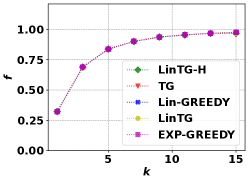
(a) movie60 $\kappa$

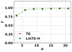
(b) movie5000 $\kappa$

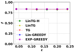
(c) movie60 $\epsilon$

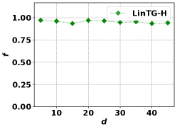
(d) movie500 d

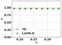
(e) movie5000 $\epsilon$

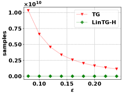
(f) movie5000 $\epsilon$

Figure 2: The experimental results of running the algorithms on instances of movie recommendation on the subsets of MovieLens 25M dataset with $n=60$, $d=5$ (”movie60”) and $n=5000$, $d=30$ (”movien5000”), and different datasets with different value of $d$.

Appendix D Technical Lemmas and Details

D.1 Matrix Computations and Runtime

In this section, we present the missing discussions on the implementation and runtime of the matrix inverse and multiplications in the main paper.

Inverse of matrix. Notice that all of the subroutine algorithms presented in the main paper keep track of $\textbf{A}_{t}^{-1}$ throughout the algorithm. From Lemma 11, we can see that the inverse of $(\textbf{A}_{t}+\textbf{x}\textbf{x}^{T})$ can be computed as

$$(\textbf{A}_{t}+\textbf{x}\textbf{x}^{T})^{-1}=\textbf{A}_{t}^{-1}-\frac{(\textbf{A}_{t}^{-1}\textbf{x})(\textbf{A}_{t}^{-1}\textbf{x})^{T}}{1+\textbf{x}^{T}\textbf{A}_{t}^{-1}\textbf{x}},$$

for any $\textbf{x}\in U$. This step takes $O(d^{2})$ in time complexity.

D.2 Technical Lemmas

Proposition 5.

(Proposition 1 in Soare et al. [2014]). Suppose the feature vector set is denoted as $\mathcal{X}$ with $|\mathcal{X}|=n$. Let $\hat{\textbf{w}}_{t}$ be the solution to the least-squares problem and let $\textbf{A}_{t}=\textbf{X}_{t}^{T}\textbf{X}_{t}$, and assume the noise variable $\xi_{t}$ is $R$-sub-Gaussian. Assume $\mathcal{Y}$ is a subset of $\mathbb{R}^{d}$ with that $|\mathcal{Y}|=Y$. Then for all $\textbf{y}\in\mathcal{Y}$ and any fixed sequence $\textbf{x}_{t}$, we have that with probability at least $1-\delta$, it holds that

$$|\textbf{y}^{T}(\hat{\textbf{w}}_{t}-\textbf{w})|\leq R||\textbf{y}||_{(\textbf{A}_{t})^{-1}}\sqrt{2\log(\frac{\pi^{2}t^{2}Y}{3\delta})}$$

for all $t>0$.

Proposition 1. Let $\hat{\textbf{w}}_{t}^{\lambda}$ be the solution to the regularized least-squares problem with regularizer $\lambda$ and let $\textbf{A}_{t}^{\lambda}=\textbf{X}_{t}^{T}\textbf{X}_{t}+\lambda\textbf{I}$. Then for every adaptive sequence $\textbf{X}_{t}$ such that at any step t, $\textbf{x}_{a_{t}}$ only depends on past history, we have that with probability at least $1-\delta$, it holds that for all $t\geq 0$ and all $\textbf{y}_{t}\in\mathbb{R}^{d}$ that only depends on past history up to time $t$,

$$|\textbf{y}_{t}^{T}(\hat{\textbf{w}}_{t}^{\lambda}-\textbf{w})|\leq||\textbf{y}_{t}||_{(\textbf{A}_{t}^{\lambda})^{-1}}C_{t},$$

where $C_{t}$ is defined as

$$C_{t}=R\sqrt{2\log\frac{\det(\textbf{A}_{t}^{\lambda})^{\frac{1}{2}}\det(\lambda I)^{-\frac{1}{2}}}{\delta}}+\lambda^{\frac{1}{2}}S.$$

Moreover, if $||\textbf{x}_{a_{t}}||\leq L$ holds for all $t>0$, then

$$C_{t}\leq R\sqrt{d\log(\frac{1+tL^{2}/\lambda}{\delta})}+\lambda^{\frac{1}{2}}S.$$

Proof.

Let us denote the history up to time t as $\mathcal{H}_{t}$, then by Cauchy–Schwarz inequality, we have that for each fixed time $t$

$$P(|\textbf{y}_{t}^{T}(\hat{\textbf{w}}_{t}^{\lambda}-\textbf{w})|\leq||\textbf{y}||_{(\textbf{A}_{t}^{\lambda})^{-1}}C_{t},\forall\textbf{y}_{t}\text{ depend on }\mathcal{H}_{t}|\mathcal{H}_{t})\geq P(||\hat{\textbf{w}}_{t}^{\lambda}-\textbf{w}||_{(\textbf{A}_{t}^{\lambda})^{-1}}\leq C_{t}|\mathcal{H}_{t})$$

It then follows that

$$P(|\textbf{y}_{t}^{T}(\hat{\textbf{w}}_{t}^{\lambda}-\textbf{w})|\leq||\textbf{y}||_{(\textbf{A}_{t}^{\lambda})^{-1}}C_{t},\forall\textbf{y}_{t}\text{ depend on }\mathcal{H}_{t})\geq P(||\hat{\textbf{w}}_{t}^{\lambda}-\textbf{w}||_{(\textbf{A}_{t}^{\lambda})^{-1}}\leq C_{t}).$$

From Theorem 2 in Abbasi-Yadkori et al. [2011], we can see that with probability at least $1-\delta$, at any step $t$, $||\hat{\textbf{w}}_{t}^{\lambda}-\textbf{w}||_{(\textbf{A}_{t}^{\lambda})^{-1}}\leq C_{t}$. Therefore, by applying this result and taking a union bound over all time step $t$, we can prove the result in the proposition. ∎

Lemma 11.

(Woodbury formula. ) The inverse of matrix $A+UCV$ can be computed as

$$(A+UCV)^{-1}=A^{-1}-A^{-1}U(C^{-1}+VA^{-1}U)^{-1}VA^{-1}.$$

Lemma 12.

(Abbasi-Yadkori et al. [2011], Lemma 10) Let the maximum $l_{2}$-norm of the feature vectors be denoted as $L$. The determinant of matrix $\textbf{A}_{t}$ is bounded as

$$det(\textbf{A}_{t})\leq(\lambda+tL^{2}/d)^{d}$$

Lemma 13.

For any vector $\textbf{x}_{1},\textbf{x}_{2}...\textbf{x}_{m}\in\mathbb{R}^{d}$ and $\textbf{y}\in\mathbb{R}^{d}$ and , if we set $p_{a}^{*}$ to be

$$p_{a}^{*}=\frac{|w^{*}_{a}|}{\sum_{a^{\prime}=1}^{m}|w^{*}_{a^{\prime}}|},$$

where $w^{*}_{a^{\prime}}$ is the optimal solution of the linear program in (5) below

$$\arg\min_{\{w_{a}\}}\sum_{a=1}^{m}|w_{a}|\qquad s.t.\qquad\textbf{y}=\sum_{a=1}^{m}w_{a}\textbf{x}_{a}.$$ (19)

Then $p_{a}^{*}$ is also the asymptotic optimal solution of the optimization problem below when $n\rightarrow\infty$.

$$\arg\min_{\{p_{a}\}}\leavevmode\nobreak\ \textbf{y}^{T}(\sum_{a\in[m]}p_{a}\textbf{x}_{a}\textbf{x}_{a}^{T}+\frac{\lambda}{n}I)^{-1}\textbf{y}$$

$$s.t.\leavevmode\nobreak\ \sum_{a\in[m]}p_{a}=1.$$

Moreover, we have that

$$\sqrt{\textbf{y}^{T}(\sum_{a\in[m]}p_{a}^{*}\textbf{x}_{a}\textbf{x}_{a}^{T})^{-1}\textbf{y}}\leq\rho,$$

where $\rho$ is the optimal value of the optimization problem in (19).

Proof.

The proof can be found in Appendix B in Xu et al. [2018], so we omit the proof here. ∎

Lemma 14.

Suppose $x\in\mathbb{R}$ and $x\geq 2$, if we have $x\geq\frac{2}{a}\log\frac{2}{a}$, then it holds that

$$\frac{\log x}{x}\leq a$$

Proof.

Since $y=\frac{\log x}{x}$ is decreasing when $x\geq 2$, if $x>\frac{2}{a}\log\frac{2}{a}$, then we have

$$\frac{\log x}{x}<\frac{a}{2}\cdot\frac{\log(\frac{2}{a}\log\frac{2}{a})}{\log\frac{2}{a}}\leq a.$$

∎

Lemma 15.

Suppose $x,a,b\in\mathbb{R}_{+}$, if we have $x\leq a+b\log x$, then it holds that

$$x\leq 2a+2b\log b.$$

References

• Abbasi-Yadkori etΒ al. [2011] Yasin Abbasi-Yadkori, DΓ‘vid PΓ‘l, and Csaba SzepesvΓ‘ri. Improved algorithms for linear stochastic bandits. Advances in neural information processing systems, 24, 2011.
• Badanidiyuru and VondrΓ‘k [2014] Ashwinkumar Badanidiyuru and Jan VondrΓ‘k. Fast algorithms for maximizing submodular functions. In Proceedings of the twenty-fifth annual ACM-SIAM symposium on Discrete algorithms, pages 1497–1514. SIAM, 2014.
• Bateni etΒ al. [2017] MohammadHossein Bateni, Hossein Esfandiari, and Vahab Mirrokni. Almost optimal streaming algorithms for coverage problems. In Proceedings of the 29th ACM Symposium on Parallelism in Algorithms and Architectures, pages 13–23, 2017.
• Chen etΒ al. [2017] Lin Chen, Andreas Krause, and Amin Karbasi. Interactive submodular bandit. Advances in Neural Information Processing Systems, 30, 2017.
• Chen etΒ al. [2014] Shouyuan Chen, Tian Lin, Irwin King, MichaelΒ R Lyu, and Wei Chen. Combinatorial pure exploration of multi-armed bandits. Advances in neural information processing systems, 27, 2014.
• Crawford etΒ al. [2019] Victoria Crawford, Alan Kuhnle, and MyΒ Thai. Submodular cost submodular cover with an approximate oracle. In International Conference on Machine Learning, pages 1426–1435. PMLR, 2019.
• Degenne etΒ al. [2020] RΓ©my Degenne, Pierre MΓ©nard, Xuedong Shang, and Michal Valko. Gamification of pure exploration for linear bandits. In International Conference on Machine Learning, pages 2432–2442. PMLR, 2020.
• El-Arini and Guestrin [2011] Khalid El-Arini and Carlos Guestrin. Beyond keyword search: discovering relevant scientific literature. In Proceedings of the 17th ACM SIGKDD international conference on Knowledge discovery and data mining, pages 439–447. ACM, 2011.
• Even-Dar etΒ al. [2002] Eyal Even-Dar, Shie Mannor, and Yishay Mansour. Pac bounds for multi-armed bandit and markov decision processes. In Computational Learning Theory: 15th Annual Conference on Computational Learning Theory, COLT 2002 Sydney, Australia, July 8–10, 2002 Proceedings 15, pages 255–270. Springer, 2002.
• Harper and Konstan [2015] FΒ Maxwell Harper and JosephΒ A Konstan. The movielens datasets: History and context. Acm transactions on interactive intelligent systems (tiis), 5(4):1–19, 2015.
• Hassidim and Singer [2017a] Avinatan Hassidim and Yaron Singer. Robust guarantees of stochastic greedy algorithms. In International Conference on Machine Learning, pages 1424–1432. PMLR, 2017a.
• Hassidim and Singer [2017b] Avinatan Hassidim and Yaron Singer. Submodular optimization under noise. In Conference on Learning Theory, pages 1069–1122. PMLR, 2017b.
• Hiranandani etΒ al. [2020] Gaurush Hiranandani, Harvineet Singh, Prakhar Gupta, IftikharΒ Ahamath Burhanuddin, Zheng Wen, and Branislav Kveton. Cascading linear submodular bandits: Accounting for position bias and diversity in online learning to rank. In Uncertainty in Artificial Intelligence, pages 722–732. PMLR, 2020.
• Horel and Singer [2016] Thibaut Horel and Yaron Singer. Maximization of approximately submodular functions. Advances in neural information processing systems, 29, 2016.
• Kalyanakrishnan etΒ al. [2012] Shivaram Kalyanakrishnan, Ambuj Tewari, Peter Auer, and Peter Stone. Pac subset selection in stochastic multi-armed bandits. In ICML, volumeΒ 12, pages 655–662, 2012.
• Karimi etΒ al. [2017] Mohammad Karimi, Mario Lucic, Hamed Hassani, and Andreas Krause. Stochastic submodular maximization: The case of coverage functions. Advances in Neural Information Processing Systems, 30, 2017.
• Kempe etΒ al. [2003] David Kempe, Jon Kleinberg, and Γ‰va Tardos. Maximizing the spread of influence through a social network. In Proceedings of the ninth ACM SIGKDD international conference on Knowledge discovery and data mining, pages 137–146, 2003.
• Leskovec etΒ al. [2007] Jure Leskovec, Andreas Krause, Carlos Guestrin, Christos Faloutsos, Jeanne VanBriesen, and Natalie Glance. Cost-effective outbreak detection in networks. In Proceedings of the 13th ACM SIGKDD international conference on Knowledge discovery and data mining, pages 420–429. ACM, 2007.
• Lin and Bilmes [2011] Hui Lin and Jeff Bilmes. A class of submodular functions for document summarization. In Proceedings of the 49th Annual Meeting of the Association for Computational Linguistics: Human Language Technologies-Volume 1, pages 510–520. Association for Computational Linguistics, 2011.
• Lindgren etΒ al. [2016] ErikΒ M. Lindgren, Shanshan Wu, and AlexandrosΒ G. Dimakis. Leveraging sparsity for efficient submodular data summarization. In Advances in Neural Information Processing Systems 29: Annual Conference on Neural Information Processing Systems, pages 3414–3422, 2016.
• Nemhauser etΒ al. [1978] GeorgeΒ L Nemhauser, LaurenceΒ A Wolsey, and MarshallΒ L Fisher. An analysis of approximations for maximizing submodular set functionsβ€”i. Mathematical programming, 14:265–294, 1978.
• Parambath etΒ al. [2018] ShameemΒ Puthiya Parambath, Nishant Vijayakumar, and Sanjay Chawla. Saga: A submodular greedy algorithm for group recommendation. In Proceedings of the AAAI Conference on Artificial Intelligence, volumeΒ 32, 2018.
• Peng [2021] Binghui Peng. Dynamic influence maximization. Advances in Neural Information Processing Systems, 34:10718–10731, 2021.
• Singla etΒ al. [2016] Adish Singla, Sebastian Tschiatschek, and Andreas Krause. Noisy submodular maximization via adaptive sampling with applications to crowdsourced image collection summarization. In Proceedings of the AAAI Conference on Artificial Intelligence, volumeΒ 30, 2016.
• Soare etΒ al. [2014] Marta Soare, Alessandro Lazaric, and RΓ©mi Munos. Best-arm identification in linear bandits. Advances in Neural Information Processing Systems, 27, 2014.
• Takemori etΒ al. [2020] Sho Takemori, Masahiro Sato, Takashi Sonoda, Janmajay Singh, and Tomoko Ohkuma. Submodular bandit problem under multiple constraints. In Conference on Uncertainty in Artificial Intelligence, pages 191–200. PMLR, 2020.
• Tschiatschek etΒ al. [2014] Sebastian Tschiatschek, RishabhΒ K Iyer, Haochen Wei, and JeffΒ A Bilmes. Learning mixtures of submodular functions for image collection summarization. Advances in neural information processing systems, 27, 2014.
• Xu etΒ al. [2018] Liyuan Xu, Junya Honda, and Masashi Sugiyama. A fully adaptive algorithm for pure exploration in linear bandits. In International Conference on Artificial Intelligence and Statistics, pages 843–851. PMLR, 2018.
• Yu etΒ al. [2016] Baosheng Yu, Meng Fang, and Dacheng Tao. Linear submodular bandits with a knapsack constraint. In Proceedings of the AAAI Conference on Artificial Intelligence, volumeΒ 30, 2016.
• Yue and Guestrin [2011] Yisong Yue and Carlos Guestrin. Linear submodular bandits and their application to diversified retrieval. Advances in Neural Information Processing Systems, 24, 2011.