Physical consequences of gauge optimization in quantum open systems evolutions

Abstract

On its own, the invariance by gauge transformations of Markovian master equations has mostly played a mathematical or computational role in the evaluation of quantum open system dynamics. So far, the fixation of a particular gauge has only gained physical meaning when correlated with additional information such as the results of measurements carried on over the system or the environment in so-called quantum trajectories. Here, we show that gauge transformations can be exploited, on their own, to optimize practical physical tasks. To do so, first, we describe the inherent structure of the underlying symmetries in quantum Markovian dynamics and present a general formulation showing how they can be used to change the measurable values of physical quantities. We then analyze examples of optimization in quantum thermodynamics and, finally, we discuss the practical implementation of the optimized protocols in terms of quantum trajectories.

In physics, invariance properties can generally be explored to discover new traits of a certain system as well as to gather deeper insights on the phenomena behind it. In many cases, they are related to symmetries of the system either derived from fundamental principles, such as the relation between invariance and conservation laws shown in Noether’s Theorem [1], or from the redundancy of degrees of freedom in the fundamental theory, such as the derivation of the electromagnetic fields from a vector and a scalar potentials [2].

In this work, we will be concerned with invariance properties arising from a lack of knowledge over the detailed structure of the system or of its interaction with external degrees of freedom, from now on referred as the environment. We will particularly focus on dynamics governed by master equations in the Gorini - Kossakowski - Sudarshan - Lindblad (GKSL) form [3]. This ignorance can be fundamental, when one does not have enough access to the system and/or to the environment, or it can be by design, when only the dynamics of the system, for example, is relevant for the physical quantities of interest. In any case, the lack of knowledge is reflected in symmetry transformations of that equation, which we will call gauges in the same sense of the electromagnetic potentials.

This gauge invariance becomes even richer when measurements are allowed, causing unavoidable back actions on the measured system. In this case, not only may physical quantities depend on the fixated gauge, but so may the single realization dynamics of the system itself, eventually affecting the behaviour of intrinsic system’s properties such as coherence [4, 5], entanglement [6, 7, 8] and quantum computational power [9]. Examples are widely found in the topic of quantum control [10, 11, 12], where proper monitoring strategies are used to drive a quantum state through specifically designed trajectories in time, known as quantum trajectories [13].

Earlier works have either exploited the differences in gauge selection to drive quantum systems through particular dynamics, in the case of quantum trajectories, or have pointed out apparent inconsistencies [14], caused by different gauges, in the definition of thermodynamic quantities such as heat and work. None of them, however, have analysed the gauge dependence in quantum open systems from an optimization perspective.

More specifically, whenever a given quantum protocol relies on gauge dependent quantities, one can naturally search for the best gauge to improve its performance. Moreover, since each gauge is related to a particular environmental monitoring scheme, identifying the improving one already indicates how to carry on the optimized protocol.

In this work, we put together these two elements by presenting a systematic and generic way to exploit gauge dependent physical quantities in order to improve quantum tasks. We then give two examples of gauge selected optimizations: the first in the energy flux and the second in the asymptotic stored ergotropy, both in low dimensional quantum systems.

.1 Dynamics invariance and gauge strategies

We begin by assuming a $d-$dimensional system $\rm S$ subject to a free Hamiltonian $H_{0}$ and coupled to its environment $\rm E$ in such a way that its dynamics is given by the following Markovian master equation:

$$\dot{\rho}(t)=-i[H,\rho(t)]+\sum_{\mu}\left(L_{\mu}\rho(t)L_{\mu}^{\dagger}-\frac{1}{2}\{L_{\mu}^{\dagger}L_{\mu},\rho(t)\}_{+}\right),$$ (1)

where $\{A,B\}_{+}=AB+BA$ is the anti-commutator and we make $\hbar=1$ for simplicity. In this equation, the interaction between $\rm S$ and $\rm E$ is manifested both as a correction of energy in $\rm S$, already comprised in $H$, and a non-unitary part given by the so-called Lindblad operators $L_{\mu}$. Even though the set $\{H,L_{\mu}\}$ derives both from the quantum state of $\rm E$ and the specificity of its interaction with $\rm S$, master equation (1) only describes the effective action on $\rm S$ due to the presence of the environment. In many physical applications, the details about $\rm E$ are either unknown or irrelevant and this effective description is all we need in order to evaluate the time evolution of meaningful physical quantities in the system.

This lack of knowledge, however, means that the set of operators $\{H,L_{\mu}\}$ is not uniquely fixed, leaving master equation (1) invariant under gauge transformations. In fact, one may define new operators

$$L_{\mu}\rightarrow L^{\prime}_{\mu}=U_{\mu\nu}L_{\nu}+\Gamma_{\mu},$$ (2)

with implicit summation on $\nu$, which will maintain the evolution of $\rho(t)$ invariant provided $H$ is transformed accordingly: $H\rightarrow H^{\prime}=H+\delta\!H$, where

$$\delta\!H=\dfrac{1}{2i}\left(\Gamma_{\mu}^{*}U_{\mu\nu}L_{\nu}-\Gamma_{\mu}U_{\mu\nu}^{*}L_{\nu}^{\dagger}\right)+\phi.$$ (3)

Here, $U_{\mu\nu}$ are the entries of a unitary matrix, $\Gamma_{\mu}$ are arbitrary complex numbers, $\phi$ is a real number and, in general, the set of parameters $\{U_{\mu\nu},\Gamma_{\mu},\phi\}$ can also be time dependent. Note that the gauge invariance has two important physical consequences: first, it shows that, for any given time evolution of S, there are infinitely many different ways to define how energy and information is exchanged with E, encoded in the change of the operators $L_{\mu}$, and to split the interaction energy between them, represented by the corresponding transformation in what is considered the system’s energy $H$. Second, it also means that there are infinitely many different maps, and hence, purifications of this dynamics that generate the same average behavior for the state of the system.

In fact, these purifications have a clear physical interpretation whenever it is possible to monitor changes in the environment [15]. To address that, we recall the unravelling of Eq. (1) into quantum trajectories by expanding the time variation of $\rho(t)$ into small finite time steps dt and rewriting the equation in the form $\rho(t+dt)=J_{0}\rho(t)J_{0}^{\dagger}+J_{\mu}\rho(t)J_{\mu}^{\dagger}$.

The so-called Kraus jump operators $J_{\mu}\equiv\sqrt{dt}L_{\mu}$ identify what happens to the system when a particular change $\mu$ is detected in the environment in the interval $dt$, while $J_{0}=\mathbb{1}-iHdt-\frac{dt}{2}L_{\mu}^{\dagger}L_{\mu}$ is applied when no change is detected. The set $\{J_{0},J_{\mu}\}$ corresponds to a POVM applied to the system in each time step $dt$ and the average over all possible outcomes of the measurements over the environment recovers the time evolution of the state of the system: $\rho(t+dt)=\sum_{i}p_{i}(t)J_{i}\rho(t)J_{i}^{\dagger}$, with $p_{i}(t)=\operatorname{Tr}\left[J_{i}^{\dagger}J_{i}\rho(t)\right]$ being the probability that the jump $J_{i}$ occurs at time $t$.

There is a direct connection between different environmental monitoring strategies and the gauge invariance of Eq. (1). The most general redefinition of strategy (POVM) corresponds to changing the set of jump operators as $J_{\mu}\rightarrow J^{\prime}_{\mu}=U_{\mu\nu}J_{\nu}+\sqrt{dt}\Gamma_{\mu}$. The transformation of the set $\{J_{\mu}\}$ is equivalent to that found in Eq. (2) and the gauge invariant master equation is obtained when averaging out on the modified POVM as long as the no-jump operator is modified accordingly, $J_{0}\rightarrow J^{\prime}_{0}=J_{0}-dt\left(\Gamma_{\mu}^{\ast}U_{\mu\nu}L_{\nu}+\frac{\Gamma_{\mu}^{\ast}\Gamma_{\mu}}{2}-i\phi\right)$. This modification corresponds to the addition of $\delta H$ as prescribed in (3).

It is straightforward to show that the set of transformations $\left\{H,L_{\mu}\right\}\rightarrow\left\{H^{\prime},L^{\prime}_{\mu}\right\}$ defines a group action operation which maintains the evolution for $\rho(t)$ unchanged, i.e., exclusive functions of $\rho(t)$ cannot distinguish between $\left\{H,L_{\mu}\right\}$ and $\left\{H^{\prime},L^{\prime}_{\mu}\right\}$ as long as they are connected by the transformations (2) and (3). Nonetheless, quantities that also depend on $\{H,L_{\mu}\}$ may not be gauge invariant and a natural question arises: can one exploit this gauge dependence to probe relevant phenomena or to enhance physical protocols?

For this to happen, these quantities have to rely on specific partitions of the master equation. In other words, consider a physical quantity $\mathcal{F}(t)$ defined as a functional of the system operators, say $\mathcal{F}(t)={\mathcal{F}}[\{H(t),L_{\mu}(t)\},\rho(t)]$. If $\mathcal{F}(t)$ is not gauge invariant, it means that different sets $\{H^{\prime}(t),L_{\mu}^{\prime}(t)\}$ may generate ${\mathcal{F}}^{\prime}(t)={\mathcal{F}}(\{H^{\prime}(t),L_{\mu}^{\prime}(t)\},\rho(t))\neq{\mathcal{F}}(t)$ for the same $\rho(t)$. In this case, the value ${\mathcal{F}}^{\prime}$(t) will explicitly depend on the gauge parameters $\{U_{\mu\nu}(t),\Gamma_{\mu}(t),\phi(t)\}$ and a specific gauge, or equivalently, a set of parameters can be chosen in order to optimize ${\mathcal{F}}^{\prime}(t)$ for a given task.

Note that finding the optimal gauge in general can be a very difficult problem to solve given that it involves optimizing over infinite sets of possible parameters in each time step of the evolution of the system. In practice, however, the task may be simplified by imposing restrictions. For example, some sets may be impossible to implement in a specific experimental setup whereas, sometimes, the task itself may require simpler optimizations. We proceed to show two examples that have been showing up quite often in the context of developing quantum technologies and where the optimization can be carried on.

.2 Energy flux in small quantum systems

A clear-cut example of a gauge dependent quantity is found when we calculate the time variation of the internal energy of a system evolving according to Eq. (1), defined by $\mathcal{P}=\partial_{t}\operatorname{Tr}\left(H\rho\right)$, where $\mathcal{P}$ stands for the energy flux into or out of the system. Given the dependence of $\mathcal{P}$ with $H$ it is clear that different sets $\left\{H,L_{\mu}\right\}$ will result in different values for $\mathcal{P}(t)$.

In particular, one can ask which gauge maximizes or minimizes the energy flux in the system by calculating $\mathcal{P}(t)$ for all possible alternatives. For a system evolving according to Eq. (1), a change of gauge $\left\{H,L_{\mu}\right\}\rightarrow\left\{H^{\prime},L^{\prime}_{\mu}\right\}$ causes a change of flux $\mathcal{P}^{\prime}=\mathcal{P}+\delta\mathcal{P}_{G}$ where the extra gauge contribution is given by

$$\delta\mathcal{P}_{G}=i\langle{[H,\delta\!H]}\rangle+\operatorname{Re}{\langle{L_{\mu}^{\dagger}[\delta\!H,L_{\mu}]}\rangle}+\langle\partial_{t}\delta\!H\rangle.$$ (4)

Optimizing $\mathcal{P}^{\prime}$ for any given task is equivalent to optimizing $\delta\mathcal{P}_{G}$ over different gauge parameters sets $\{U_{\mu\nu},\Gamma_{\mu},\phi\}$. Furthermore, since each gauge is associated to a particular environmental monitoring setting and, hence, to a different family of POVMs acting on the system, once the optimal gauge is chosen for any given task, the gauge fixation automatically defines the respective optimal environmental observation scheme and the possible trajectories for the system.

For instance, in the case of a qubit coupled to a thermal bath at inverse temperature $\beta$, the typical gauge to describe its dynamics is given by the set $\{H=\tfrac{\omega}{2}\hat{\sigma}_{z}$, $L_{\pm}=\sqrt{\gamma_{\pm}}\hat{\sigma}_{\pm}\}$, where $\hat{\sigma}_{-}$ ( $\hat{\sigma}_{+}$) corresponds to the system losing (gaining) a quantum of energy $\omega$ to (from) the bath at rate $\gamma_{-}$ ($\gamma_{+}$) and $\frac{\gamma_{+}}{\gamma_{-}}=e^{-\beta\hbar\omega}$. A general transformation following Eqs. (2) and (3) results in

$$\delta\!H=\frac{\alpha(t)}{2}\hat{\sigma}_{+}+\frac{\alpha^{\ast}(t)}{2}\hat{\sigma}_{-},$$ (5)

with $\alpha=-i\left(\Gamma_{\mu}^{\ast}U_{\mu+}\sqrt{\gamma_{+}}-\Gamma_{\mu}U_{\mu-}^{\ast}\sqrt{\gamma_{-}}\right)$, a complex number defined by the gauge. The eventual time dependence of the parameters is implied. Note that $\delta\!H=\textrm{Re}(\alpha)\hat{\sigma}_{x}-\textrm{Im}(\alpha)\hat{\sigma}_{y}$ is defined on the plane perpendicular to $H$ in the Bloch Sphere.

For the sake of simplicity, let us now restrict ourselves to the set of gauges where $\alpha(t)=|\alpha|e^{i\theta(t)}$, with $|\alpha|$ constant. After some straightforward algebra, one obtains a gauge contribution to the variation of $\mathcal{P}$ given by

$$\delta\!\mathcal{P}_{G}=\dfrac{\alpha(t)}{2}\left[i(\omega+\dot{\theta})-\dfrac{\gamma_{+}+\gamma_{-}}{2}\right]\rho_{ge}(t)+h.c.,$$ (6)

where $\rho_{ij}(t)=\bra{i}\rho(t)\ket{j}$ stands for the coherence of the system ($i\neq j)$ in the eigenbasis of $H$. Note that, in this example, the final form (6) indicates a physical interpretation to each gauge: when the time variation of the internal energy of the qubit is considered, a general transformation on the set $\{H,L_{\mu}\}$ acts as a transferrer, which transforms the evolution of the initial coherences in the system into a power contribution at each time $t$.

In particular, if the system has no initial coherence in the eigenbasis of $H$, then $\rho_{eg}(t)=0$ throughout the evolution and the choice of gauge is irrelevant. Also note that the choice of the best gauge, encoded in $\alpha(t)$, depends on the phase of $\rho_{eg}(0)$. In fact, one can choose the sign of $\delta\mathcal{P}_{G}(t)$ by simply changing the relative phase between $\alpha(t)$ and $\rho_{ge}(0)$.

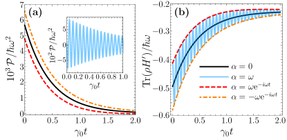
Figure 1: Time evolution of energy flux (a) and internal energy (b) of different gauges leading to the same evolution of a qubit. In all curves, $\gamma_{0}=10^{-2}\omega$, $k_{B}T_{0}=0.2\hbar\omega$ and $k_{B}T_{f}=\hbar\omega$.

Finally, Eq. (6) indicates that one can find monitoring schemes where the exchanged energy per unit of time between the system and its environment can be controlled for any desired task at the expense of any coherences which are present in the initial state of the system.

Figure 1 shows the energy flux and internal energy of the qubit for different gauge parameters. The black curve corresponds to $\alpha=0$, i.e. the original set $\{H,L_{\mu}\}$. The colored curves correspond to different gauges, where $|\alpha|$ is kept fixed and $\theta$ is allowed to change. The lightblue curve corresponds to a time independent gauge, where the time evolution of the coherences naturally creates the oscillatory behaviour in the internal energy of the system. In this case, $\theta$ only defines the initial phase of the oscillation. On the other hand, by allowing $\theta$ to change in time one is able to coherently interfere either constructively (red, dashed curve) or destructively (orange, dot-dashed curve) with the time oscillations of the coherences of the qubit, accelerating or slowing down the rate at which energy is pumped into the system through the reservoir. In all curves, an initial pure state $\ket{\psi(0)}=\sqrt{p_{g}^{0}}\ket{g}+\sqrt{p_{e}^{0}}\ket{e}$ evolves through the same (gauge invariant) $\rho(t)$ and asymptotically reaches a fully mixed Gibbs state $\rho^{\rm as}=p_{g}^{f}|g\rangle\langle g|+p_{e}^{f}|e\rangle\langle e|$ where, $p_{i}^{j}$ is given by a Boltzmann distribution with energy $E_{i}=\langle i|H|i\rangle$ and inverse temperature $\beta_{j}$. We are also considering jump ratios $\gamma_{+}=\gamma_{0}\overline{n}$ and $\gamma_{-}=\gamma_{0}(\overline{n}+1)$, where $\overline{n}=(1-e^{-\beta_{f}\omega})^{-1}$.

.3 Ergotropy on a quantum battery

Another example of gauge dependent quantity is the ergotropy stored in a quantum battery [16, 17, 18, 19, 20, 21, 22, 23, 24]. Quantum batteries are devices able to store energy in quantum systems and, as the ordinary ones, deliver this energy as useful work [25, 26, 27, 28, 29]. Ergotropy is the maximum amount of energy that can be extracted from the system via unitary transformations and it is given by:

$$\mathcal{E}[H,\rho]=\sum_{i}p_{i}^{\rm dec}\left(\bra{p_{i}^{\rm dec}}H\ket{p_{i}^{\rm dec}}-E_{i}\right),$$ (7)

where $p_{i}^{\rm dec}$ are the eigenvalues of $\rho$ labelled in order of decreasing magnitude, while $E_{i}$ are the eigenvalues of $H$ labelled in order of increasing magnitude. Equation (7) makes explicit that the ergotropy is also a gauge dependent physical quantity, as a function of $H$, and therefore it may change as a consequence of gauge variation.

For instance, consider again the same qubit subjected to a thermal bath of inverse temperature $\beta$, for which the asymptotic state, achieved when $t\gg\gamma_{\pm}^{-1}$, is the same Gibbs state previously described, $\rho^{\rm as}_{ii}=\dfrac{e^{-\beta E_{i}}}{\sum_{j=g,e}e^{-\beta E_{j}}}$. Given that $\rho^{\rm as}_{ee}<\rho^{\rm as}_{gg}$, $\rho^{\rm as}$ has no stored ergotropy in the gauge $\{H,L_{\mu}\}$, which can be straightforwardly checked from Eq. (7). This is not necessarily true, however, if a different gauge $\{H^{\prime},L^{\prime}_{\mu}\}$ is picked to drive the dynamics. The change in the Hamiltonian of the system means that $\rho^{\textrm{as}}$ and $H^{\prime}=H+\delta\!H$ will not commute anymore and, as a consequence, $\rho^{\textrm{as}}$ may store ergotropy with respect to the new Hamiltonian.

The eigenstates of $H^{\prime}$ are written in terms of the original eigenstates as

$$\ket{\psi_{+}}=\sqrt{n_{1}}\ket{g}+e^{-i\theta}\sqrt{n_{2}}\ket{e},$$ (8)

$$\ket{\psi_{-}}=\sqrt{n_{2}}\ket{g}-e^{-i\theta}\sqrt{n_{1}}\ket{e},$$ (9)

with the eigenvalues $E_{\pm}=\pm\dfrac{\omega}{2}[2G(\alpha)+1]$, where $G(\alpha)\equiv\dfrac{1}{2}\sqrt{1+\dfrac{|\alpha|^{2}}{\omega^{2}}}-\dfrac{1}{2}$, $n_{1}=\frac{G(\alpha)}{2G(\alpha)+1}$ and $n_{2}=\frac{G(\alpha)+1}{2G(\alpha)+1}$. It is very easily checked that for $\alpha\rightarrow 0$ (i.e., no gauge transformation) we recover the original states.

The gauge transformed ergotropy is given by

$$\mathcal{E}[H^{\prime},\rho^{\textrm{as}}]=G(\alpha)\hbar\omega\left[\rho_{gg}^{\textrm{as}}-\rho_{ee}^{\textrm{as}}\right].$$ (10)

Note that the addition of $\delta\!H$ per se does not change the asymptotic value of the internal energy of the system, since the new Hamiltonian $\delta\!H$ is completely off-diagonal in the eigenbasis of $\rho^{\textrm{as}}$, implying that $\textrm{Tr}[\rho^{\textrm{as}}H^{\prime}]=\textrm{Tr}[\rho^{\textrm{as}}H]$. This indicates that no extra energetic resource is being transmitted into the system by $\delta\!H$. However, $\rho^{\textrm{as}}$ is not a thermal equilibrium state anymore and the energy to keep it out of equilibrium and, therefore, to store ergotropy in it, is injected by the transformed reservoir.

As mentioned before, each gauge can be associated to a particular physical implementation of quantum trajectories, each one corresponding to a POVM acting on the system and depending on measurements performed over the environment. In particular, different POVMs for the evolution of qubits in contact with thermal-like reservoirs have been discussed in  [6, 9]. There, each jump operator $J_{\pm}$ can be associated to the detection of a corresponding circularly polarized photon emitted by the system into the environment. Direct photon-detection distinguishing both circularly polarized light modes implement the original set $\{H,L_{\mu}\}$ on the system. Rotating the polarization of the modes before detecting the emitted photon implements the unitary transformations $U_{\mu\nu}$ over the original $L_{\mu}$ components of the set, according to equation (2). On the other hand, combining each mode with a local oscillator field (a coherent state of amplitude $s_{\mu}$) at a highly reflective mirror (of reflectivity $r\sim 1$), implements the addition of the $\Gamma_{\mu}$ term in the same transformation, where $\Gamma_{\mu}\propto\sqrt{1-r}\times s_{\mu}$.

The logic behind it is simple: the rotation of the polarization recombines the modes and therefore the jumps to which they are associated, whereas their combination with the local oscillator at the highly reflective mirror superposes the modes with an external photon source in such a way that a click on a given detector imposes a superposition of a corresponding jump (the photon coming from the system) and identity (the photon coming from the external source) acting on the system. Finally, an external classical field directly driving the $|g\rangle\rightarrow|e\rangle$ transition implements the required $\delta\!H$ to complete the set for the new gauge.

I Conclusion

In this work, we have proposed a systematic protocol to explore symmetries in quantum Markovian master equations beyond their mathematical elegance. It consists of identifying physical quantities that are gauge dependent and affect the performance of given practical tasks and searching for the best set of gauge parameters that meets the intended objective. The asymptotic stored energy and the energy flux through the evolution of the system were the two examples depicted here but the protocol is general and any figure of merit that varies according to the chosen set is suitable for optimization. Further examples to be explored in the future include heat exchanged with the environment, entropy production, efficiency of thermal machines, preparation of target oriented asymptotic states, etc.

The method also allows to identify the resource being exploited in each different gauge. In the examples worked on the paper, the optimization of the energy flux requires initial quantum coherence to be consumed throughout the evolution whereas the storing of ergotropy comes from the athermality of the asymptotic state. The identified resources are consistent with previous results found in the literature [30, 31, 32, 33, 34, 35].

In addition, the unravelling of the Lindblad master equation in terms of quantum trajectories indicates an experimental way to probe the optimization method: each gauge translates into a set of jump operators which act on the system at infinitesimal time steps and identifies the possible evolutions of the system in each realization. Finding the optimal gauge parameters automatically informs us the best set of measurements that must be carried on over the environment in order to physically implement the desired optimization. This meets direct applications in any area where engineering and control of a given reservoir can be explored to enhance physical protocols, as well as areas where continuous monitoring of the environment is performed in order to feedback control a given evolution. We followed up by providing an example on how to experimentally implement the gauge transformations discussed in our qubit example. Note that, nowadays, there are plenty of atomic (real and artificial) systems where the conditions for such experiments are met including atoms coupled to open cavities [36, 37, 38], superconducting qubits connected to waveguides [39], quantum dots embedded in nanowires [40], NV-centers in photonic crystals [41], etc.

Finally, a first idea on how to generalize this protocol starts by wondering what are the effects of letting the gauge parameters $U_{\mu\nu}$ and $\Gamma_{\mu}$ assume time dependence beyond the linear, which is allowed by the symmetries involved. Furthermore, we also let open the question whether this procedure could be performed on other types of master equations, such as those describing non-Markovian evolutions or even master equations describing classical systems. At last, it may also be of interest to study the relations between these symmetries and their applications with fundamental physical questions related to the thermodynamics of quantum systems.

- [1] V.I. Arnold, Mathematical Methods of Classical Mechanics (Graduate Texts in Mathematics, 2nd ed., Springer-Verlag, 1989);
- [2] J.D. Jackson, Classical Electrodynamics, (3rd Ed., John Wiley & Sons, 1999);
- [3] H.-P. Breuer & F. Petruccione, The Theory of Open Quantum Systems, (Oxford University Press, New York, 2002);
- [4] H. J. Carmichael, L. Tian, and P. Kochan, “Decay of quantum coherence using quantum trajectories”, in Optical Society of America Annual Meeting, Technical Digest Series (Optica Publishing Group, 1992), paper MFF4.
- [5] Li C-X. “Protecting the Quantum Coherence of Two Atoms Inside an Optical Cavity by Quantum Feedback Control Combined with Noise-Assisted Preparation”. Photonics. 2024; 11(5):400.
- [6] A. R. R. Carvalho and M. F. Santos, “Distant Entanglement Protected through Artificially Increased Local Temperature”, New J. Phys. 13, 013010 (2011).
- [7] E. Mascarenhas, D. Cavalcanti, V. Vedral, and M. F. Santos, “Physically Realizable Entanglement by Local Continuous Measurements”, Phys. Rev. A 83, 022311 (2011).
- [8] A. R. R. Carvalho and J. J. Hope, “Stabilizing Entanglement by Quantum-Jump-Based Feedback”, Phys. Rev. A 76, 010301(R)(2007).
- [9] M. F. Santos, M. Terra Cunha, R. Chaves, and A. R. R. Carvalho, “Quantum Computing with Incoherent Resources and Quantum Jumps”, Phys. Rev. Lett. 108, 170501 (2012).
- [10] F. Sakuldee, S. Milz, F. A. Pollock, and K. Modi, Non-Markovian “Quantum Control as Coherent Stochastic Trajectories”, J. Phys. A: Math. Theor. 51, 414014 (2018).
- [11] C. Brif, M. D. Grace, M. Sarovar, and K. C. Young, “Exploring Adiabatic Quantum Trajectories via Optimal Control”, New J. Phys. 16, 065013 (2014).
- [12] L. Magrini, P. Rosenzweig, C. Bach, A. Deutschmann-Olek, S. G. Hofer, S. Hong, N. Kiesel, A. Kugi, and M. Aspelmeyer, “Real-Time Optimal Quantum Control of Mechanical Motion at Room Temperature”, Nature 595, 373 (2021).
- [13] A. J. Daley, “Quantum Trajectories and Open Many-Body Quantum Systems”, Advances in Physics 63, 77 (2014).
- [14] F. Nicacio and R. N. P. Maia, “Gauge Quantum Thermodynamics of Time-Local Non-Markovian Evolutions”, Phys. Rev. A 108, 022209 (2023).
- [15] Genoni, M.G., Mancini, S. & Serafini, A. “General-dyne unravelling of a thermal master equation”. Russ. J. Math. Phys. 21, 329–336 (2014).
- [16] Z. Beleño, M. F. Santos, and F. Barra, “Laser Powered Dissipative Quantum Batteries in Atom-Cavity QED”, arXiv:2310.09953.
- [17] Y. V. de Almeida, T. F. F. Santos, and M. F. Santos, “Cooperative Isentropic Charging of Hybrid Quantum Batteries”, Phys. Rev. A 108, 052218 (2023).
- [18] T. F. F. Santos, Y. V. de Almeida, and M. F. Santos, “Vacuum-Enhanced Charging of a Quantum Battery”, Phys. Rev. A 107, 032203 (2023).
- [19] T. F. F. Santos and M. F. Santos, “Efficiency of Optically Pumping a Quantum Battery and a Two-Stroke Heat Engine”, Phys. Rev. A 106, 052203 (2022).
- [20] Y.-Y. Zhang, T.-R. Yang, L. Fu, and X. Wang, “Powerful Harmonic Charging in a Quantum Battery”, Phys. Rev. E 99, 052106 (2019).
- [21] C.-K. Hu et al., “Optimal Charging of a Superconducting Quantum Battery”, Quantum Sci. Technol. 7, 045018 (2022).
- [22] D. Ferraro, M. Campisi, G. M. Andolina, V. Pellegrini, and M. Polini, “High-Power Collective Charging of a Solid-State Quantum Battery”, Phys. Rev. Lett. 120, 117702 (2018).
- [23] C. Cruz, M. F. Anka, M. S. Reis, R. Bachelard, and A. C. Santos, “Quantum Battery Based on Quantum Discord at Room Temperature”, Quantum Sci. Technol. 7, 025020 (2022).
- [24] F. Barra, “Dissipative Charging of a Quantum Battery”, Phys. Rev. Lett. 122, 210601 (2019).
- [25] A. E. Allahverdyan, R. Balian, and T. M. Nieuwenhuizen, “Maximal Work Extraction from Finite Quantum Systems”, EPL 67, 565 (2004).
- [26] D. Morrone, M. A. C. Rossi, and M. G. Genoni, “Daemonic Ergotropy in Continuously Monitored Open Quantum Batteries”, Phys. Rev. Appl. 20, 044073 (2023).
- [27] B. Çakmak, “Ergotropy from Coherences in an Open Quantum System”, Phys. Rev. E 102, 042111 (2020).
- [28] G. Francica, F. C. Binder, G. Guarnieri, M. T. Mitchison, J. Goold, and F. Plastina, “Quantum Coherence and Ergotropy”, Phys. Rev. Lett. 125, 180603 (2020).
- [29] G. Francica, “Quantum Correlations and Ergotropy”, Phys. Rev. E 105, L052101 (2022).
- [30] R. Rubboli and M. Tomamichel, “Fundamental Limits on Correlated Catalytic State Transformations”, Phys. Rev. Lett. 129, 120506 (2022).
- [31] V. Narasimhachar and G. Gour, “Resource Theory under Conditioned Thermal Operations”, Phys. Rev. A 95, 012313 (2017).
- [32] A. Martin Alhambra, “Non-Equilibrium Fluctuations and Athermality as Quantum Resources”, Doctoral, UCL (University College London), 2017.
- [33] M. Horodecki and J. Oppenheim, “Quantumness in the Context of Resource Theories”, Int. J. Mod. Phys. B 27, 1345019 (2013).
- [34] G. Gour, “Role of Quantum Coherence in Thermodynamics”, PRX Quantum 3, 040323 (2022).
- [35] B. de L. Bernardo, “Unraveling the Role of Coherence in the First Law of Quantum Thermodynamics”, Phys. Rev. E 102, 062152 (2020).
- [36] Q. A. Turchette, C. J. Hood, W. Lange, H. Mabuchi, and H. J. Kimble, “Measurement of Conditional Phase Shifts for Quantum Logic”, Phys. Rev. Lett. 75, 4710 (1995).
- [37] Q. A. Turchette, R. J. Thompson, and H. J. Kimble, “One-Dimensional Atoms”, Applied Physics B-Lasers and Optics 60, S1 (1995).
- [38] A. Auffeves-Garnier, C. Simon, J.-M. Gerard, and J.-P. Poizat, “Giant Optical Nonlinearity Induced by a Single Two-Level System Interacting with a Cavity in the Purcell Regime”, Phys. Rev. A 75, 053823 (2007).
- [39] O. Astafiev, A. M. Zagoskin, A. A. Abdumalikov, Y. A. Pashkin, T. Yamamoto, K. Inomata, Y. Nakamura, and J. S. Tsai, “Resonance Fluorescence of a Single Artificial Atom”, Science 327, 840 (2010).
- [40] L. Leandro, J. Hastrup, R. Reznik, G. Cirlin, and N. Akopian, “Resonant Excitation of Nanowire Quantum Dots”, Npj Quantum Inf 6, 1 (2020).
- [41] J. P. Hadden et al., “Integrated Waveguides and Deterministically Positioned Nitrogen Vacancy Centers in Diamond Created by Femtosecond Laser Writing”, Opt. Lett., OL 43, 3586 (2018).