Abstract

Using the Kreuzer-Skarke database of 4-dimensional reflexive polytopes, we systematically constructed a new database of orientifold Calabi-Yau threefolds with $h^{1,1}(X)\leq 12$. Our approach involved non-trivial $\mathbb{Z}_{2}$ involutions, incorporating both divisor exchanges and multi-divisor reflections acting on the Calabi-Yau threefolds. Each proper involution results in an orientifold Calabi-Yau threefolds and we constructed $320,386,067$ such examples. We developed a novel algorithm that significantly reduces the complexity of determining all the fixed loci under the involutions, and clarifies the types of O-planes. Our results show that under proper involutions, the majority of cases end up with $O3/O7$-plane systems, and most of these further admit a naive Type IIB string vacua. Additionally, a new type of free action was determined. We also computed the smoothness and the splitting of Hodge numbers in the $\mathbb{Z}_{2}$-orbifold limit for these orientifold Calabi-Yau threefolds.

1 Introduction

String theory, aiming to describe the fundamental forces of the universe within a single theoretical framework, often requires compactification from higher dimension to lower dimension to properly describe observable phenomena. Among various compactification methods, four-dimensional $\mathcal{N}=1$ supersymmetric compactifications are particularly well-studied due to their theoretical tractability. Within this framework, the compactification manifold usually is a Calabi-Yau threefold $X$. Compactifying type IIA or type IIB string theories on Calabi-Yau threefolds $X$ yields an $\mathcal{N}=2$ supersymmetry theory in four dimensions. Therefore, to break half of the supersymmetry to $\mathcal{N}=1$, and to address the necessity of O-planes for tadpole cancellation when including open string modes such as D-branes and fluxes, an additional orientifold projection with a proper $\mathbb{Z}_{2}$ involution $\sigma$ acting on the Calabi-Yau threefold $X$ is required. In this paper, we employ a new strategy and a novel algorithm, significantly extending our previous work [1, 2], to construct orientifold Calabi-Yau threefolds with $h^{1,1}(X)\leq 12$, considering both non-trivial divisor exchange involutions and multi-divisor reflection involutions.

Our investigation focuses specifically on Type IIB orientifold geometries, where an orientifold projection $\mathcal{O}$ involves two key components: the worldsheet parity $\Omega_{p}$ and a diffeomorphism map $\sigma$ acting on the Calabi-Yau threefolds $X$, referred to as the involution. Notably, the involution $\sigma$ such that $\sigma^{2}=1$ must meet certain criteria to preserve supersymmetry, thus it has to be isometric and holomorphic [3, 4]. Under this action, the compactification manifold may feature fixed loci, corresponding to orientifold planes (O-planes), whose structure depends on the specific orientifold system, such as the $O5/O9$ and $O3/O7$ systems:

$${\cal O}=\begin{cases}\Omega_{p}\,\sigma\qquad&{\rm with}\quad\sigma^{*}(J)=J\,,\quad\sigma^{*}(\Omega_{3})=+\Omega_{3},\quad$O5/O9$\,\,{\rm system},\\[2.84544pt] (-1)^{F_{L}}\,\Omega_{p}\,\sigma\qquad&{\rm with}\quad\sigma^{*}(J)=J\,,\quad\sigma^{*}(\Omega_{3})=-\Omega_{3},\quad$O3/O7$\,\,{\rm system},\end{cases}$$ (1)

Each of the involution $\sigma(\sigma^{2}=1)$ defines a new Calabi-Yau in the orbifold limit unless it is a free action. In general, the involution $\sigma$ splits the cohomology groups $H^{p,q}(X/\sigma^{*})$ into eigenspaces of even and odd parity:

$$H^{p,q}(X/\sigma^{*})=H^{p,q}_{+}(X/\sigma^{*})\oplus H^{p,q}_{-}(X/\sigma^{*}).$$ (2)

For reflection involution, the equivariant cohomology $h^{1,1}_{-}(X)$ is always vanishing while for divisor exchange involution it is usually $h^{1,1}_{-}(X)>0$:

$$\sigma=\begin{cases}{{\rm Reflection:}}\,\,\{\,x_{i}\leftrightarrow-x_{i},\cdots\,\}&h^{1,1}_{-}(X)=0\\[2.84544pt] {{\rm Exchange\,\,involution:}}\,\,\{\,x_{i}\leftrightarrow x_{j},\cdots\,\}&{h^{1,1}_{-}(X)>0}\end{cases}$$ (3)

Orientifold Calabi-Yau threefolds play an important role in string phenomenology for both particle physics and string cosmology. Recently, in the context of the swampland conjecture(first proposed in [5, 6] and see [7, 8, 9, 10] for a detail review), various corrections, such as warping correction, loop correction, and $\alpha^{\prime}$ correction, put a constraint on the orientifold Calabi-Yau that can be used for compactification to construct de-Sitter vacua in the Large Volume Scenario (LVS) [11, 12, 13, 14, 15, 16, 17]. In order to solve the chirality issue when combining the local particle physics and moduli stabilization [18], tuning on fluxed-instanton on the divisors was considered [19, 20, 21]. There is also a selection rule determining which kinds of orientifold Calabi-Yau threefolds can support the global embedding of Standard Model at the toric singularity in the geometry, where both reflections with $h^{1,1}_{-}(X)=0$ and divisor exchange involutions with $h^{1,1}_{-}(X)>0$ were considered [22, 23, 24, 25, 26, 27, 28, 29, 30, 31].

Recently, several databases of orientifold Calabi-Yau threefolds have been established. Initially, the orientifold Calabi-Yau threefolds with divisor exchange involutions were constructed for $h^{1,1}(X)\leq 4$ [1] using maximal triangulations from the Kreuzer-Skarke dataset of reflexive four-dimensional polyhedra [32]. This toric construction was extended to $h^{1,1}(X)\leq 6$, with explicitly fixed loci and types of O-planes in [2] based on the Calabi-Yau database [33]. Given the fact that Calabi-Yau manifold compatible with the proper exchange involution are rare in the entire database, it is a very good signal to apply machine learning tecnique to identify those polytopes which can result in an orientifold Calabi-Yau threefold [34]. Such orientifold structure from the polytope perspective was later studied in [35]. The orientifold Calabi-Yau threefolds with single divisor reflection involutions were considered in [36]. More general free quotient in the toric Calabi-Yau with $h^{1,1}(X)\leq 3$ were systematically explored in [37]. In the context of Complete Intersection Calabi-Yau 3-folds (CICYs) embedded in products of projective spaces [38], people start to construct a landscape of orientifold vacua [39] from the most favorable description of CICY 3-folds database [40]. General free quotients have been classified and studied in the case of CICY 3-folds  [41, 42, 43, 44].

Despite significant progress in constructing orientifold Calabi-Yau threefolds, technical challenges persist when extending to higher $h^{1,1}(X)$. The first obstacle is the huge number of Calabi-Yau threefolds itself. Using graph theory and neural network techniques, it has been shown that the number of fine, regular, star triangulations (FRSTs) of four-dimensional reflexive polytopes is bounded by $\mathcal{O}(10^{928})$, with topologically inequivalent ones bounded by $\mathcal{O}(10^{428})$ [45]. Although divisor exchange involution compatible with the geometry are rare in the database, one can always perform the multi-divisor reflection involutions, which is missing in literatures. Each involution results in an orientifold Calabi-Yau manifold for which we must determine the fixed loci and types of O-planes. However, the computational complexity of determining these fixed loci often exceeds the capabilities of current computer. Therefore, developing a more efficient algorithm is crucial for extending our previous work to a much larger database with higher $h^{1,1}(X)$, including both divisor exchange involutions and reflections, and clarifying ambiguities in determining the fixed loci.

In this paper, we extend and improve upon previous work in several key areas, including large-scale construction, increased efficiency, and clarification of ambiguities:

1. We extend our classification bound up to $h^{1,1}(X)=12$ in the Calabi-Yau database constructed from the Kreuzer-Skarke list [32]. For $h^{1,1}(X)\leq 7$, we expand our analysis to hypersurfaces in all possible maximal projective crepant partial (MPCP) desingularizations. For $8\leq h^{1,1}(X)\leq 12$, we randomly choose some favorable polytopes for each hodge number as in [36]. The number of toric triangulations we will analyze increases by one order of magnitude from $653,062$ [2] to $6,696,714$.

2. We expand our classification to cover both divisor exchange involutions and multi-divisor reflection involutions. First, we determine the individual topology of divisors in each toric Calabi-Yau threefold and refine our algorithm to identify all proper divisor exchange involutions, resulting in a total of $156,709$ proper divisor exchange involutions. For multiple reflection involutions, we explore all possible single, double, and triple divisor reflections for Calabi-Yau threefolds with $h^{1,1}(X)\leq 6$. For $h^{1,1}(X)=7$, we analyze all single reflections, and randomly chosen 15 double and 15 triple reflections. For $8\leq h^{1,1}(X)\leq 12$, we randomly select 15 triple reflections in addition to single reflections. In total, we examine $320,229,358$ different types of reflections. Consequently, we determine their equivariant cohomology (Hodge number splitting) in the $\mathbb{Z}_{2}$-orbifold limit.

   Since each of the such involutions results in an orientifold Calabi-Yau manifold, combining both types of involutions, we constructed a total $320,386,067$ of orientifold Calabi-Yau threefolds in our new database (https://github.com/GroupofXG/anewcydatabase/), which is three orders of magnitude ($\mathcal{O}(10^{3})$) larger than our previous work [2].

3. We employed new strategy to identify all possible fixed loci under divisor exchanges and reflection involutions. This enables us to identify the positions of various types of O-planes, which are crucial for D-brane constructions. The new algorithm significantly reduces the calculation complexity for determining fixed loci by more than five order of magnitude ($\mathcal{O}(10^{5})$) for a standard Calabi-Yau threefolds with $h^{1,1}(X)=7$ and will be more efficient for higher $h^{1,1}(X)$.

4. We classify freely acting involutions on Calabi-Yau threefolds into two categories: those with a fixed locus in the ambient space that does not intersect with the Calabi-Yau threefold and those even without a fixed locus in the ambient space.

5. In orientifold Calabi-Yau threefolds featuring the $O3/O7$-system, we proceed to classify the so-called “naive orientifold Type IIB string vacua” by considering the D3 tadpole cancellation condition when putting eight $D7$-branes on top of $O7$-plane.

This paper is organized as follows: In Section 2.1, we briefly review the construction of Calabi-Yau threefolds as hypersurfaces in toric varieties and how to compute the Hodge numbers of individual toric divisors. In Section 2.2, we identify all pairs of “Non-trivial Identical Divisors” (NIDs) and then present the proper divisor exchange involutions and multi-divisor reflections. The fixed-point loci on the ambient space are then identified in Section 2.3 and then restricted on the Calabi-Yau threefolds in Section 2.4. Computation complexity of the previous algorithm was described in Section 2.3.1 and great efforts were performed to introduce a new strategy to reduce the computation complexity in Section 2.3.2. This information is used to classify the involutions as either non-trivially or freely acting in Section 2.5. We illustrate the procedures via detailed examples for both divisor exchange involutions and multi-divisor reflections in Section 3 and clarify some ambiguities there. Then we summarize our results in Section 4.

2 Construct Orientifold Calabi-Yau Threefolds

2.1 Polytope, Triangulation and Divisors

The toric Calabi-Yau threefolds $X$ can generically be obtained by taking the anticanonical hypersurface in an ambient four-dimensional Gorenstein toric Fano variety, denoted by $\mathcal{A}$ [46]. First, we require a desingularized representation of our original four-dimensional ambient space $\mathcal{A}$ from the Kreuzer-Skarke database [32]. Achieving this entails smoothing out some irregularities in a four-dimensional ambient space $\mathcal{A}$, by blowing up enough of its singular points through a process called maximal projective crepant partial (MPCP) desingularization. This method involves triangulating the polar dual reflexive polytope, denoted as $\Delta^{*}$, to ensure it contains at least one fine, regular, star triangulation (FRST). Such a desingularized four-dimensional ambient toric variety could be expressed as:

$$\mathcal{A}=\frac{\mathbb{C}^{k}-Z}{\left(\mathbb{C}^{*}\right)^{k-4}\times G}\,,$$ (4)

where $Z$ is the locus of points in $\mathbb{C}^{k}$ ruled out by the Stanley-Reisner ideal $\mathcal{I}_{SR}(\mathcal{A})$, and $G$ is the stringy fundamental group. There are only 16 manifolds in the Kreuzer-Skarke list contain a non-trivial first fundamental group $G$. In many applications in physics the group $G$ can be taken to be trivial and we are left with the simple split torus action $\left(\mathbb{C}^{*}\right)^{k-4}$ in the denominator of the quotient. This torus $\mathbb{C}^{*}$ action can also take the role of an abelian gauge group acting on some two-dimensional field theory as was explained in [47] and may therefore also be called the $U(1)$ action.

We will consider the ambient space $\mathcal{A}$ as a resolved four-dimensional Gorenstein toric Fano variety whose anticanonical divisor $X=-K_{\mathcal{A}}$ represents a Calabi-Yau threefold hypersurface. Here we restrict ourselves to the so-called “favorable” description, in which the toric divisor classes on the Calabi-Yau hypersurface $X$ are all descended from ambient space $\mathcal{A}$ . The following short exact sequence and its dual sequence

$$0\rightarrow TX\rightarrow T\mathcal{A}|_{X}\rightarrow\mathcal{N}_{X/\mathcal{A}}\rightarrow 0,$$ (5)

$$0\rightarrow\mathcal{N}^{*}_{X/\mathcal{A}}\rightarrow T^{*}\mathcal{A}|_{X}\rightarrow T^{*}X\rightarrow 0,$$

can induce the long exact sequence in sheaf cohomology

(10)

From the above sequence and Dolbeault’s theorem, $H^{1}(X,T^{*}X)\cong H^{1,1}(X)\cong{\rm coker}(\alpha)\oplus{\rm ker}(\beta)$. This equivalence has two parts. One comes from the restriction of Kähler moduli from $\mathcal{A}$ to $X$, and the other comes from the kernel part. If the kernel part is empty, we call the geometry favorable and $h^{1,1}(X)={\rm dim}(H^{1,1}(X))\cong{\rm dim}({\rm Pic}(\mathcal{A}))$.

Denote $x_{i}$ as the weighted homogeneous coordinates used to define $X$ inside the ambient space $\mathcal{A}$. Then the divisor $D_{i}\equiv\{x_{i}=0\}$ defines a 4-cycle on $X$ and it is dual to a 2-cycle $\omega_{i}$, i.e., $D_{i}\in H^{1,1}(X,\mathbb{Z})$. Due to the favorability description of polytopes and geometries, all such toric divisors $D_{i}$ are irreducible on the Calabi-Yau threefolds $X$. Hence, $H_{4}(X,\mathbb{Z})$ is generated by any basis constructed from $D_{i}$, $i=1,...,k=h^{1,1}(X)+4.$ Now, the Calabi-Yau threefolds on this toric variety can be described by a polynomial in terms of the projective coordinates $\{x_{1},...,x_{k}\}$. Their torus $\left(\mathbb{C}^{*}\right)^{k-4}$ equivalence classes reads

$$(x_{1},...,x_{k})\sim(\lambda^{\mathbf{W}_{i1}}x_{1},...,\lambda^{\mathbf{W}_{ik}}x_{k})\,,$$ (11)

where $\mathbf{W}$ is the GLSM weighted matrix of rank $r=k-4$, charged under $r$ $U(1)s$.

The internal topology of these divisors play an important role in string compactification and moduli stabilization. The Hodge numbers of divisors are collectively denoted as

$$h^{\bullet}(D,\mathcal{O}_{D})=\{h^{0,0}(D),h^{1,0}(D),h^{2,0}(D),h^{1,1}(D)\}$$ (12)

For an irreducible divisor $D$, the complex conjugation $h^{p,q}(D)=h^{q,p}(D)$ and Hodge star $h^{p,q}(D)=h^{2-p,2-q}(D)$ dualities constrain the independent Hodge numbers of $D$ down to only $h^{1,0}(D),h^{2,0}(D)$, and $h^{1,1}(D)$. This calculation will be performed by using the Koszul extension to the cohomCalg package [50, 51] with the HodgeDiamond module. When we encounter difficulties with cohomCalg in calculating Hodge number of a divisor, we first calculate the Euler number $\chi(D)=\int_{D}{c_{2}(D)}$ of the divisor on the hypersurface, and then determine $h^{1,0}(D)$ and $h^{2,0}(D)$ by calculating the trivial line bundle cohomology of the divisor $h^{\bullet}(D,\mathcal{O}_{D})$ [52]. Then, using the expression

$$\chi(D)=\sum\limits_{i=0}^{2}(-1)^{i}\,{\rm dim}\left(H^{i}_{\rm DR}(D)\right)=\sum\limits_{p+q=0}^{2}(-1)^{p+q}\,{\rm dim}\left(H^{q}(D,\Omega^{p})\right)\,,$$ (13)

we can fix $h^{1,1}(D)$ and get the full Hodge diamond for any divisor. In our procedure for scanning divisor involutions, several types of divisors are of particular phenomenological interest:

Completely rigid divisors: The Hodge numbers of these divisors are characterized by $h^{\bullet}(D)=\{1,0,0,h^{1,1}(D)\}$ such that $h^{1,1}(D)\neq 0$. This group of divisors falls into two categories: del Pezzo surfaces, denoted by $\{\mathbb{P}^{2}\equiv dP_{0}$, $dP_{n}$, with $n=1,\dots,8\}$ and $n=h^{1,1}(D)-1$. These del Pezzo divisors are usually shrinkable depending on the diagonalizability of their intersection tensor. The shrinkable del Pezzo surface plays a crucial role to generate a non-perturbative superpotentail [53], which is important for KKLT [54] and LVS [11] construction. For those divisors with $h^{1,1}(D)>9$, they are always referred as “non-shrinkable rigid divisors”.

“Wilson” divisors: The Hodge numbers of these divisors are characterized by $h^{\bullet}(D)=\{h^{0,0}(D),h^{0,1}(D),$ $h^{0,2}(D),h^{1,1}(D)\}=\{1,h^{1,0},0,h^{1,1}\}$ with $h^{1,0}(D),\,h^{1,1}(D)\neq 0$. We will also further specify the “Exact-Wilson” divisor as $h^{\bullet}(D)=\{1,1,0,h^{1,1}\}$ with $h^{1,1}(D)\neq 0$ which are crucial for supporting poly-instanton inflation[55, 56, 57].

Deformation divisors: These divisors are characterized simply by $h^{2,0}(D)\neq 0$.

• A K3 divisor is a deformation divisor with Hodge numbers $h^{\bullet}(D)=\{1,0,1,20\}$, which is used to generate fiber inflation [58].

• A deformation divisor resembles a K3 divisor but includes an additional $h^{1,1}(X)$ deformation degree of freedom, i.e., $h^{\bullet}(D)=\{1,0,1,21\}$. We refer to this type of divisor as a type-1 special deformation divisor, denoted by $SD1$.

• In our scan, a type-2 special deformation divisor, denoted as $SD2$, frequently appears with Hodge numbers $h^{\bullet}(D)=\{1,0,2,30\}$.

2.2 Proper Involutions from Divisor Exchanges and Reflections

We expand our classification of involutions to cover both divisor exchange involutions and multi-divisor reflection involutions compared with previous work [1, 2]. For divisor exchange involutions, the map $\sigma:x_{i}\leftrightarrow x_{j}$, which swaps two homogeneous coordinates in the ambient toric variety $\mathcal{A}$, induces a holomorphic involution $\sigma^{*}:D_{i}\leftrightarrow D_{j}$ on the corresponding toric divisor cohomology classes. On favorable manifolds, this involution restricts in a straightforward way to the Calabi-Yau hypersurface $X$. We then define the even and odd parity eigendivisor classes $D_{\pm}\equiv D_{i}\pm D_{j}\in H^{1,1}_{\pm}(X/\sigma^{*})$. In general, a given geometry may allow multiple disjoint involutions $\sigma_{1},\sigma_{2},\dots,\sigma_{n}$. In this case, the full involution is given by $\sigma\equiv\sigma_{1}\circ\sigma_{2}\circ\cdots\circ\sigma_{n}$.

Consequently, it is necessary to identify the proper involution $\sigma$ that exchanges one or more pairs of divisors. These divisors should share the same topology but have different charge weights. We call such pairs of divisors as non-trivial identical divisors (NIDs) and it can be summarized as:

$$\sigma:x_{i}\leftrightarrow x_{j}\quad\Longleftrightarrow\quad\sigma^{*}:D_{i}\leftrightarrow D_{j}.$$

$$H^{\bullet}(D_{i})\cong H^{\bullet}(D_{j}),\quad\mathcal{O}(D_{i})\neq\mathcal{O}(D_{j})$$ (14)

Furthermore, such involution should satisfy the symmetry of Stanley-Reisner ideal $\mathcal{I}_{SR}(\mathcal{A})$ and the symmetry of the linear ideal $\mathcal{I}_{lin}(\mathcal{A})$. The first symmetry ensures that the involution is an automorphism of $\mathcal{A}$, preserving the exceptional divisors from resolved singularities. The second symmetry ensures that the defining polynomial of the Calabi-Yau manifold remains homogeneous under the involution. Putting these two together, the involution should be a symmetry of the Chow-group:

$$A^{\bullet}(\mathcal{A})\cong\frac{\mathbb{Z}(D_{1},\cdots,D_{k})}{\mathcal{I}_{lin}(\mathcal{A})+\mathcal{I}_{SR}(\mathcal{A})}\,,$$ (15)

Due to the favorability condition on the Calabi-Yau threefold hypersurface we have

$$A^{1}(\mathcal{A})\cong H^{1,1}(\mathcal{A})\cong{\rm Pic}(\mathcal{A})\cong{\rm Pic}(X)\cong H^{1,1}(X)\cong A^{1}(X)\,,$$ (16)

and thus the toric triple intersection number defined in the Chow ring $A^{4}(X)$ should also be required to be invariant under the involution $\sigma$. Only when an involution, exchanging pairs of NIDs, satisfying all these requirements described above, can be called a “proper” involution.

For reflection involutions on divisors, these are pulled back from the coordinate reflections on the ambient space $\mathcal{A}$:

$$\sigma:x_{i}\leftrightarrow-x_{i}\quad\Longleftrightarrow\quad\sigma^{*}:D_{i}\leftrightarrow-D_{i}.$$ (17)

The situation is much simpler since it always satisfies the conditions for “proper” involutions. So we will explore possible single, double and triple divisor reflections for Calabi-Yau threefolds.

One crucial difference between divisor exchange and reflection involutions is the Hodge number splitting structure. The holomorphic condition requires that the pullback $\sigma^{*}$ maps $(p,q)$-forms on $X$ to $(p,q)$-forms on $\mathcal{A}$. This is also true at the level of cohomology as the Dolbeault operator $\bar{\partial}$ commutes with the pullback $\sigma^{*}$. This implies that in the orientifold limit, the dimensions of equivariant cohomology split as:

$$h^{p,q}(X/\sigma^{*})=h^{p,q}_{+}(X/\sigma^{*})\,+h^{p,q}_{-}(X/\sigma^{*})\,.$$ (18)

The reflection involution $\sigma^{*}:D_{i}\leftrightarrow-D_{i}$ acts trivially on the divisor classes and thus manifestly does not contribute to $h^{1,1}_{-}(X/\sigma^{*})$. However, the divisor exchange involution $\sigma^{*}:D_{i}\leftrightarrow D_{j}$ acts non-trivially on the divisor classes and thus contributes to the non-trivial odd cohomology $h^{1,1}_{-}(X/\sigma^{*})$. In order to determine whether the $h^{1,1}_{\pm}(X/\sigma^{*})$ split, we should expand the Kähler form $J$, which has even parity under $\sigma$ and thus $J\in H^{1,1}_{+}(X)$, in terms of those divisor classes. By defining even and odd parity eigendivisors $D_{\pm}=D_{i}\pm D_{j}$, one can expand $J$ in the new divisor basis including $D_{+}\in H^{1,1}_{+}$. This leads to a specific form for $J$ and we can read off the Hodge number splitting of $h^{1,1}_{\pm}$ by the number of independent expansion coefficients.

Furthermore, we can determine the Hodge number splitting of $h^{2,1}_{\pm}(X/\sigma^{*})$ in the $\mathbb{Z}_{2}$-orbifold limit by Lefschetz fixed point theorem [59, 60]. In general the $\mathbb{Z}_{2}$ involution $\sigma$ induced a fixed-point set ${\cal F}$. Due to the hodge number splitting eq.(18), we can define the Leftschetz number of $\sigma^{*}$ as $L(\sigma^{*},X)$:

$$L(\sigma^{*},X)\equiv\sum_{i}(-)^{i}(b^{i}_{+}-b^{i}_{-})=\chi({\cal F})\,,$$

$${\rm where\quad\quad} \chi(\cal F)\supset\begin{cases}\,\,\chi(O7)=\int_{O7}\,c_{2}(O7)\,,\\ \,\,\chi(O5)=\int_{O5}\,c_{1}(O5)\,,\\ \,\,\chi(O3)=\int_{O3}\,c_{0}(O3)\,=N_{O3}\,.\end{cases}$$ (19)

$b_{\pm}^{i}$ is the splitted Betti numbers and $\chi({\cal F})$ is the Euler number of the fixed locus ${\cal F}$. There is a very useful theorem to calculate the Euler number of the $\mathbb{Z}_{2}$-orbifold space:

$$\chi(X/{\sigma^{*}})=\frac{1}{2}\,\big{(}L(\sigma^{*},X)+\chi(X)\big{)}\,=\sum_{i}(-)^{i}(b^{i}_{+}).$$ (20)

This number is the average of the Lefschetz number and the Euler number of $X$. Then we can determine the $h^{2,1}_{-}(X/\sigma^{*})$ as:

$$h^{2,1}_{-}(X/\sigma^{*})=h^{1,1}_{-}(X/\sigma^{*})+\frac{L(\sigma^{*},X)-\chi(X)}{4}-1,$$ (21)

where for reflections $h^{1,1}_{-}(X/\sigma^{*})=0$.

For a consistent orientifold, we must ensure both $\sigma^{*}J=J$ and $\sigma^{*}\Omega_{3}=\pm\Omega_{3}$ as shown in eq.(1), where $\Omega_{3}$ is the unique holomorphic (3,0)-form on $X$. The holomorphic (3,0)-form $\Omega_{3}$ can be constructed using the homogenous coordinates [61],

$$\Omega=\frac{1}{2\pi i}\oint_{P=0}\frac{\omega\cdot\Pi_{a}V^{a}}{P},$$ (22)

where $P$ is the hypersurface polynomial and $\omega=dx^{1}\wedge\cdots\wedge dx^{k}$. The $V^{a}$ are the holomorphic vector fields that generate the gauge symmetries, determined in terms of the weights $Q^{a}_{i}$ as follows:

$$V^{a}=\Sigma_{i}Q^{a}_{i}x_{i}\frac{\partial}{\partial x_{i}}.$$ (23)

Since the hypersurface polynomial $P$ must be invariant under $\sigma$, the numerator of the integrand, denoted as $\mathcal{Q}$, determines the parity. The parity of $\mathcal{Q}$ serves as a useful cross-check to verify if the correct O-plane system is obtained under the involution.

Next, we need to determine the fixed locus under the involutions and identify the corresponding types of O-planes. This process is more technical and will be introduced in the next subsection. For now, we assume the data of O-planes is known, allowing us to verify if the orientifold Calabi-Yau manifold supports a string vacuum. In this context, we consider a simple case where the $D7$-brane tadpole cancellation condition is satisfied by placing eight $D7$-branes on top of the $O7$-plane. Consequently, we only need to check the $D3$-brane tadpole condition, which is simplified to:

$$N_{D3}+\frac{N_{\text{flux}}}{2}+N_{\rm gauge}=\frac{N_{O3}}{4}+\frac{\chi(D_{O7})}{4}\,\equiv-\,Q_{D3}^{loc}.$$ (24)

with $N_{\text{flux}}=\frac{1}{(2\pi)^{4}\alpha^{{}^{\prime}2}}\int H_{3}\wedge F_{3}$, $N_{\text{gauge}}=-\sum_{a}\frac{1}{8\pi^{2}}\int_{D_{a}}\text{tr}{\cal F}_{a}^{2}$, and $N_{D3}$, $N_{O3}$ the number of D3-branes, $O3$-planes respectively. The D3-tadpole cancellation condition requires the total D3-brane charge $Q_{D3}^{loc}$ of the seven-brane stacks and $O3$-planes to be an integer. If the involution passes this naive tadpole cancellation check, we will denote this geometry as a “naive orientifold Type IIB string vacuum”.

2.3 Putative Fixed Locus on Ambient Space $\mathcal{A}$

A smooth Calabi-Yau hypersurface $X=-K_{\mathcal{A}}$ is defined by the vanishing locus of a homogeneous polynomial $P$. The polynomial $P$ can be expressed in terms of the known vertices $m\in\Delta,n\in\Delta^{*}$ of the Newton and dual polytopes, respectively

$$P=\sum_{m\in\Delta}{a_{m}M_{m}}=0,\hskip 14.22636pt\text{where}\hskip 14.22636ptM_{m}=\prod_{i=1}^{k}{x_{i}^{\langle m,n_{i}\rangle+1}}\,.$$ (25)

where $k=h^{1,1}(X)+4$ due to the favorability. In order for the Calabi-Yau hypersurface to be invariant under the involution $\sigma$, we must restrict to the subset of moduli space in which the defining polynomial is invariant. The first step is to fix the invariant polynomial such that $P_{sym}=\sigma(P_{sym})$ in addition to $\sigma^{*}J=J$. Mathematically, this could be done by a regulation of the coefficients of the original polynomial $P$ by:

$$\left\{\begin{aligned} &a_{m}=0\qquad&&\sigma(M_{m})\notin\{M_{m}|m\ \in\ \Delta\}\\ &a_{m}=a_{n}\qquad&&\sigma(M_{m})=M_{n},n\neq m\\ &a_{m}\ {\rm\,\,generic}\qquad&&\sigma(M_{m})=M_{m}\end{aligned}\right.$$ (26)

Clearly, imposing these restrictions requires some tuning in the complex structure moduli space and this tuning may introduce singularities into the invariant polynomial $P_{sym}$. For reflection involutions, the invariant polynomial $P_{sym}$ is simply the sum of invariant monomials, where the coordinates involved in the reflections $\sigma:\{x_{i}\leftrightarrow-x_{i},x_{j}\leftrightarrow-x_{j}\dots\}$ have even powers in total, i.e., $\{x_{i}^{2}...,x_{j}^{2}...,x_{i}^{2}x_{j}^{2}...,x_{i}x_{j}...,\dots\}$.

Now we start to search for the set of points fixed under $\sigma$. We first locate the fixed-point set in the ambient space $\mathcal{A}$, and then restrict this set to the Calabi-Yau hypersurface $X$. In the following we will first describe how to find the fixed point loci for divisor exchange involution and then treat the reflection cases as special ones.

For divisor exchange involution $\sigma$, following [2], we first construct the minimal generators $\mathcal{G}$ generated by homogeneous polynomials that are (anti-)invariant under $\sigma$:

$$\mathcal{G}=\mathcal{G}_{0}\cup\mathcal{G}_{+}\cup\mathcal{G}_{-}\,.$$ (27)

where $\mathcal{G}_{0}$ is the collection of unchanged coordinates under $\sigma$. The unexchanged coordinates in $\mathcal{G}_{0}$ are known from our choice of involution. If the involution $\sigma$ exchange $n$ pairs of coordinates, to find the non-trivial even and odd parity generators in $\mathcal{G}_{+}$ and $\mathcal{G}_{-}$, we must consider not only $\sigma$, but all possible non-trivial sub-involutions given by the nonempty subsets of $\{\sigma_{1},...,\sigma_{n}\}$ of size $1\leq m\leq n$, with $\sigma_{m}:x_{i_{m}}\leftrightarrow x_{j_{m}}$. Then we denote the new coordinate in $\mathcal{G}\equiv\{y_{1},...,y_{k^{\prime}}\}$ as:

$$y_{\pm}(\mathbf{a})=x_{i_{1}}^{a_{1}}x_{i_{2}}^{a_{2}}\dotsm x_{i_{m}}^{a_{m}}\pm x_{j_{1}}^{a_{1}}x_{j_{2}}^{a_{2}}\dotsm x_{j_{m}}^{a_{m}}\,,$$ (28)

where $\mathbf{a}=(a_{1},a_{2},\dotsc,a_{m})\in\mathbb{Z}^{m}$, $k^{\prime}=|\mathcal{G}|$ is the number of definite parity polynomial generators, related to $k$ and $\sigma$, and could be smaller or bigger than $k$. The condition for homogeneity, in terms of the columns $\mathbf{w}_{i_{s}}$ and $\mathbf{w}_{j_{s}}$ of the weight matrix $\mathbf{W}$ is given by

$$a_{1}(\mathbf{w}_{i_{1}}-\mathbf{w}_{j_{1}})+a_{2}(\mathbf{w}_{i_{2}}-\mathbf{w}_{j_{2}})+\dotsb+a_{m}(\mathbf{w}_{i_{m}}-\mathbf{w}_{j_{m}})=0\,.$$ (29)

The second step is to perform a Segre embedding transforming the origianl coordinates $\{x_{i}\}$ into the new (anti-)invariant generators defined in eq.(28):

$$\{x_{1},...,x_{k}\}\mapsto\{y_{1},...,y_{k^{\prime}}\}\equiv\mathcal{G},$$ (30)

which constructs a new weight matrix $\tilde{\mathbf{W}}$ for $\{y_{i}\}$. Now we have transform the original $(k-4)\times k$ GLSM matrix $\mathbf{W}$ to a $r\times k^{\prime}$ matrix $\tilde{\mathbf{W}}$ with $r=\text{rank}(\tilde{\mathbf{W}})$, $k=h^{1,1}(X)+4$ and $k^{\prime}=|\mathcal{G}|$. Then we can find out the naive fixed point loci in the new coordinates.

After Segre embedding, we have transformed the divisor exchange involution to the reflection $\sigma:y_{i}\mapsto-y_{i}$. We can show that the corresponding coordinate exchange must force the codimension-1 subvariety defining polynomial to vanish so that $D_{i}=\{y_{i}=0\}$ is fixed. It also implies that the polynomial of every point-wise fixed codimension-1 subvariety can be generated by odd-parity generators in $\mathcal{G}_{-}$.

In general, we need to check whether the involution allows a subset of generators $\mathcal{F}\subseteq\mathcal{G}$ to vanish simultaneously. Meanwhile, the torus $\mathbb{C}^{*}$ actions provide additional $r=\text{rank}(\tilde{\mathbf{W}})$ degrees of freedom for the generators to avoid being forced to zero. More precisely, the requirement for a locus to be fixed could be represented as forcing the related generators vanish simultaneously while leaving the others transform under $\mathbb{Z}_{2}$ symmetry as usual. This is achieved by checking each subset of generators $\mathcal{F}\subseteq\mathcal{G}$ whether the following $\lambda$ system have a solution:

$$\lambda_{1}^{\tilde{W}_{1i}}\lambda_{2}^{\tilde{W}_{2i}}\dotsb\lambda_{r}^{\tilde{W}_{ri}}=\sigma(y_{i})/y_{i},\quad i=1,\dots,k^{\prime}\,{\rm and}\,\,y_{i}\notin\mathcal{F}$$ (31)

where $\lambda_{i}\in\mathbb{C}^{*}$ is the torus action and the right-hand side is equal to $\pm 1$ depending on whether the reflection involving the coordinates or not.

For reflection involution, there is no need for Segre embedding and we only need to consider a simpler system with $r=\text{rank}({\mathbf{W}})=h^{1,1}(X)$:

$$\lambda_{1}^{{W}_{1i}}\lambda_{2}^{{W}_{2i}}\dotsb\lambda_{r}^{{W}_{ri}}=\sigma(x_{i})/x_{i},\quad i=1,\dots,k\,{\rm and}\,\,x_{i}\notin\mathcal{F}\,$$ (32)

where $k=h^{1,1}(X)+4$ and the right-hand side is equal to $\pm 1$ depending on whether $\sigma$ include $x_{i}\leftrightarrow-x_{i}$.

For both divisor exchange involutions and reflections, the set in $\mathcal{F}$ is point-wise fixed on the ambient space $\mathcal{A}$ if and only if the complex $\lambda$ system equations eq.(31) and eq.(32) are solvable after imposing the related set in $\mathcal{F}$ to vanish simultaneously. We call these subsets $\mathcal{F}$ passed these check as putative fixed locus in the ambient space $\mathcal{A}$.

2.3.1 Calculation Complexity

There are two aspects of calculation complexities for determining the putative fixed locus on $\mathcal{A}$. One is the total number of subsets $\mathcal{F}\subseteq\mathcal{G}$ may be large. For divisor exchange involutions and reflections respectively, in principle there are as much as $\displaystyle\sum_{i=1}^{k^{\prime}}C_{k^{\prime}}^{i}=2^{k^{\prime}}$ and $\displaystyle\sum_{i=1}^{k}C_{k}^{i}=2^{k}$ subsets $\mathcal{F}\subseteq\mathcal{G}$ we need to solve the $\lambda\in\mathbb{C}^{*}$ system eq.(31) and eq.(32). Another complexity comes from solving the $\lambda$ system in complex field itself which we will describe below.

For divisor exchange involutions as in [2] and each of the putative fixed locus $\mathcal{F}$, in order to check whether the system eq.(31) is solvable, we define $\lambda_{i}\equiv e^{i\pi u_{i}}\in\mathbb{C}^{*}$ with $0\leq u_{i}<2$ so that the equation (31) is converted to:

$$\tilde{W}_{1i}u_{1}+\dotsb+\tilde{W}_{ri}u_{r}\equiv\left\{\begin{array}[]{rl}0\pmod{2},&y_{i}\in\mathcal{G}_{0}\cup\mathcal{G}_{+}\\ 1\pmod{2},&y_{i}\in\mathcal{G}_{-}\end{array}\right.\,.$$ (35)

and further becomes:

$$\tilde{W}_{1i}u_{1}+\dotsb+\tilde{W}_{ri}u_{r}-2q_{i}\equiv\left\{\begin{array}[]{rl}0,&y_{i}\in\mathcal{G}_{0}\cup\mathcal{G}_{+}\\ 1,&y_{i}\in\mathcal{G}_{-}\end{array}\right.$$ (38)

with $0\leq u_{i}<2$ and $q_{i}\in\mathbb{Z}$. If the new GLSM weight matrix $\tilde{W}_{ji}$ contains negative entries for a given line-bundle $\mathcal{O}(D_{i})$ corresponding to the coordinate $y_{i}$, we need to check the solvability of eq.(38) by scanning $q_{i}\in\mathbb{Z}$ in a range of

$$\left\{\begin{array}[]{rl}&{\displaystyle\sum_{j}^{r}}\eta(-{\tilde{W}}_{ji})*\tilde{W}_{ji}<q_{i}<{\displaystyle\sum_{j}^{r}}\eta({\tilde{W}}_{ji})*\tilde{W}_{ji},\,\,y_{i}\in\mathcal{G}_{0}\cup\mathcal{G}_{+}\\ &{\displaystyle\sum_{j}^{r}}\eta(-{\tilde{W}}_{ji})*\tilde{W}_{ji}\leq q_{i}<{\displaystyle\sum_{j}^{r}}\eta({\tilde{W}}_{ji})*\tilde{W}_{ji},\,\,y_{i}\in\mathcal{G}_{-}\end{array}\right.$$ (41)

where $\eta(x)$ is a STEP function such that $\eta(x)=0$ if $x<0$ and $\eta(x)=1$ for $x\geq 0$. Thus the summation in the left-hand side of eq.(41) represents the sum of the negative entries, while the right-hand side represents the sum of the positive entries. If the entries of $\tilde{W}_{ji}$ are all positive for a given line-bundle $\mathcal{O}(D_{i})$, the scanning range is simplified to:

$$0\leq q_{i}<\sum_{j}^{r}\tilde{W}_{ji}$$ (42)

Thus, the problem of determining the solvability of the $\lambda$ system transforms into determining the solvability of $u_{i}$ in eq.(38) for a given lattice point $q_{i}$ within the range defined by eq.(41) and eq.(42). If any solution is found for any lattice point $q_{i}$, then the set of generators $\mathcal{F}$ has a point-wise fixed locus.

However, this method will exhaust computational resources as $h^{1,1}(X)$ increases. For example, if all the entries of $\tilde{W}_{ji}$ are positive then the upper limit of points in the $q_{i}$ lattice that need to be tested can be estimated as:

$$\prod\limits_{i=1}^{\hat{k}^{\prime}}(\sum_{j}^{r}\tilde{W}_{j,i})\xlongrightarrow{h^{1,1}\,\,\,{\rm large}}\mathcal{O}(1-100)^{\hat{k}^{\prime}},$$ (43)

where $\hat{k^{\prime}}$ indicates the number of elements in the index set $\{1,\dots\hat{i}\dots,k^{\prime}\}$ excluding the index $i$ for $y_{i}\notin\mathcal{F}_{i}$. The total computational complexity we encounter is given by eq.(43), multiplied by the number of all possible fixed sets that need to be tested, which is $\prod\limits_{i=1}^{\hat{k}^{\prime}}(\sum_{j}^{r}\tilde{W}_{j,i})\times 2^{k^{\prime}}$.

The problem of computational complexity is the same for reflection involutions except there is no need for Segre embedding. Therefore, we change the GLSM weighted matrix in eq.(35 - 43) to $W_{ji}$ and maintain the coordinate system as $\{x_{i}\}$ with $k=h^{1,1}(X)+4$ and $\hat{k}$ the number of index set excluding the coordinates involved in reflections. Consequently, the total complexity for reflection involutions becomes $\prod\limits_{i=1}^{\hat{k}}(\sum_{j}^{r}W_{j,i})\times 2^{k}$.

Combining these two complexities in determining putative fixed locus on $\mathcal{A}$, one may encounter limitations in computational power. For instance, consider a favorable Calabi-Yau with $h^{1,1}(X)=7$ and single reflection, i.e., $k=11$ and $r=h^{1,1}(X)=7$. Even with a small average summation $\displaystyle\sum_{j}^{r}W_{j,i}=3$ for all $q_{i}$, we need to test up to $3^{10}=59,049$ $q_{i}$ lattice points for each of the $2^{11}=2,048$ possible fixed locus sets $\mathcal{F}$. This results in a total of $\mathcal{O}(10^{10})$ lattice points to be tested. For an exchange involution switch two pairs of NIDs in the same geometry, consider again a small average summation $\displaystyle\sum_{j}^{r}\tilde{W}_{j,i}=3$ for all $q_{i}$ with $k^{\prime}=15$ and $r=3$. We need to test up to $4,782,969$ $q_{i}$ lattice points for each of the $2^{15}=32,768$ possible fixed locus sets $\mathcal{F}$, totaling $\mathcal{O}(10^{12})$ points. For a geometry with $h^{1,1}(X)=20$ and moderate average summation $\displaystyle\sum_{j}^{r}\tilde{W}_{j,i}=10$, exchanging five pairs of NIDs (which often results in $k^{\prime}\sim 34$ and $r\sim 10$) forces us to check up to $\mathcal{O}(10^{33})\times\mathcal{O}(10^{10})$ lattice points in extreme cases, which is beyond current computational capabilities. Even though in many cases we don’t need to exhaust all the possible lattice points, this remains a significant challenge for general scans and we need to solve these problems..

2.3.2 New Algorithm

There are two directions to reduce the complexity of calculation. One is to reduce the scanning space of $q_{i}$ lattice points, the other is to reduce the number of the possible fixed loci needed to be test. For the first purpose, we initially solve the $\lambda$ system in the real number field to identify some putative fixed loci and then search in the complex number field to check whether we miss some solutions. In this procedure, based on the fixed loci obtained in the real number field, we can significantly reduce the number of possible fixed loci we need to check.

Real number $\lambda$ system

Solving the $\lambda$ system in real number field first can extremely reduce the number of $q_{i}$ lattice points that need to bw checked. This new algorithm focuses on $\lambda$, i.e., eq.(31-32), rather than eq.(38) with focus on $u_{i}$ and $q_{i}$ with a larger parameter space. By concentrating on real $\lambda$ values, we only need to consider two relevant value: $\lambda=\pm 1$, or equivalently, setting $u_{i}$ in $\lambda=e^{i\pi u_{i}}\in\mathbb{C}^{*}$ to $0$ and $1$. Consequently, the largest dimension of parameter space for solving the $\lambda$ system is reduced to

$$2^{r}\quad{\rm with\,\,\,}\left\{\begin{array}[]{rlr}&r=\text{rank}(\tilde{\mathbf{W}})\leq h^{1,1}(X)&{\rm exchange\,\,involution}\\ &r=\text{rank}({\mathbf{W}})=h^{1,1}(X)&{\rm reflection\,\,involution}\end{array}\right.\,$$ (46)

Now, let us consider the example with $h^{1,1}(X)=7$ described above to see the extent of the parameter space reduction. Compared to $59,049$ or $4,782,969$ parameter spaces that need to be scanned for each of possible fixed loci set in the complex space, we only need to consider $2^{7}=128$ different values of $\lambda$ at most. For the case with $h^{1,1}(X)=20$, we reduce the dimension of parameter space from $\mathcal{O}(10^{33})$ to $2^{20}=1,048,576$.

The advantage of the new approach is that it reduce the parameter space of solving system significantly. This reduction depends on the rank of $\tilde{\mathbf{W}}$ through eq.(46), which is smaller than $h^{1,1}(X)$, rather than eq.(43) which is sensitive to the GLSM matrix and $k^{\prime}$ (which in most cases is larger than $h^{1,1}(X)$). For reflection involutions, the only difference is that we treat ${\mathbf{W}}$ with $r=h^{1,1}(X)$ and $k=h^{1,1}(X)+4$ instead.

However, this is not the end of the story. At this stage, some putative fixed loci may be missed if, for a given test set $\mathcal{F}$, there is no choice of $\lambda=\pm 1$ that satisfy eq.(31-32), but solutions may exist for complex $\lambda=e^{i\pi u}\in\mathbb{C}^{*}$ with $0\leq u_{i}<2$. Therefore the next step is to search in complex number field to identify any missed fixed loci. Fortunately, the fixed loci computed in the real number system can be used to reduce the number of possible loci that need to be tested.

Before we go to the detail of how to reduce the possible fixed locus we need to check, we give a remark on the GLSM weighted matrix in our new algorithm. In [2], the entries of GLSM matrix are chosen to be non-negative by restricting the matrix to the positive orthant $\mathbb{Z}_{\geq 0}^{k}$. This is achieved by intersecting two polyhedrons: the first is generated by lines specified by the elements of kernel of vectors defining the ambient space $\mathcal{A}$, and the second is generated by rays specified by the unit basis vectors. There are two shortages of this approach for determining the fix loci. First, with non-negative entries of ${\mathbf{W}}$, the summation $\displaystyle\sum_{j}^{r}W_{j,i}$ shown in eq.(43) will also be large, contributing to the tardiness of fixed loci computation, making it a nearly impossible. Second, when intersecting two polyhedron, the parity of the the first polyhedron may change, affecting the results of finding fixed loci in the real $\lambda$ system. Although such parity change in GLSM weighted matrix do not affect determination of the fixed loci, since we eventually check all solutions of eq.(31-32) in the complex number field, it is much more convenient to keep the parity throughout the entire calculation. Therefore in this paper we will start from the standard output of PALP [62] and SAGE [63] to get the GLSM weighted matrix with negative entries from the vertex in the dual-polytope $\Delta^{*}$ as shown in the Kreuzer-Skarke list [32].

After utilizing our new algorithm to get the fixed loci in real number system, yielding the same result for single divisor reflection as in [36], we use these fixed loci to simplify the computation of the entire fixed locus on the Calabi-Yau threefold in complex space.

Reduce possible sets of $\mathcal{F}$

There are four classes of subsets of $\mathcal{F}$ that can help reduce the number of possible fixed loci we need to test in the complex $\lambda$ system.

1. If a subset $\mathcal{F}_{i}$ we get in real $\lambda$ system is a fixed locus, then any set containing it would also be a fixed locus.

2. Apply the Stanley-Reisner ideal $\mathcal{I}_{SR}$ to rule out subsets $\mathcal{F}_{i}$ which should not vanish simultaneously.

3. Apply the linear ideal $\mathcal{I}_{lin}$ to rule out some possible combinations of subsets $\mathcal{F}_{i}$ to test the solvability.

4. If a subset $\mathcal{F}_{i}$ is not a fixed locus, then all subsets contained within $\mathcal{F}_{i}$ will not be fixed loci.

The first three classes of sets $\mathcal{F}_{i}$ are loci that allow us to rule out sets containing them when searching for new solutions in complex $\lambda\in\mathbb{C}^{*}$ system, thus belonging to the same type. The last class of sets $\mathcal{F}_{i}$ helps us rule out those sets contained within it. Let us first explain how these two types of special loci work and then estimate how effectively they can help reduce the complexity.

Consider the type one sets first. For known fixed loci $\mathcal{F}_{i}$ in real $\lambda$ system, they remian fixed loci in complex $\lambda\in\mathbb{C}^{*}$ system, and any sets $\mathcal{F}_{i}^{\prime}$ containing $\mathcal{F}_{i}$ will also be fixed loci. This is because the real number solution ${\boldsymbol{\lambda}}$ of eq.(31-32) for loci $\mathcal{F}_{i}$ is also the solution for loci within $\mathcal{F}_{i}^{\prime}$, as the later has fewer constraints in complex $\lambda$ system. One can further reduce the test sets $\mathcal{F}_{i}$ by using the SR ideal $\mathcal{I}_{SR}$. The SR ideal describes sets that cannot vanish simultaneously on the ambient space, so there is no need to test sets $\mathcal{F}_{i}$ contain elements of the SR ideal. The third class of sets applies to divisor exchange involutions, where new bases are introduced after Segre embedding. Here the minimal hypersurface generators $\{y_{i}\}$ are not independent, and their linear relations, encoded in the linear ideal $\mathcal{I}_{lin}$, can be used to rule out some possible loci. For example, suppose there are new basis $y_{1},y_{2},y_{3}$ consist of old bases $\{x_{i}\}$ in such way: $\{y_{1}=x_{1}*x_{2}+x_{3}*x_{4},y_{2}=x_{1}*x_{4},y_{3}=x_{2}*x_{3}\}$, then such linear relations can be used to rule out sets $\mathcal{F}_{i}$ in which any combination of $y_{2}$ and $y_{3}$ are fixed, but $y_{1}$ is not fixed.

Finally, the scanning procedure can be further simplified by recognizing that if a set of points is not fixed, then neither is any set containing it. Thus, if the simultaneous vanishing of a set of generators is not fixed, neither is the vanishing of any subset. For example, if $\mathcal{F}_{i}=\{n_{i},n_{j},n_{k}\}$ is an non-fixed locus, then all subsets $\{\{n_{i}\},\{n_{j}\},\{n_{k}\},\{n_{i},n_{j}\},\{n_{i},n_{k}\},\{n_{k},n_{j}\}\}$ contained in $\mathcal{F}_{i}$ are also not fixed and don’t need to be tested. Therefore, we begin our scan with the largest set of generators and work our way down. Usually, the largest set we can choose has four generators, as their simultaneous vanishing defines a set of isolated points on the ambient space $\mathcal{A}$. However, if $\mathcal{F}_{i}$ vanish on the invariant polynomial $P_{sym}$, we will relax the number of generators to five or more.

Efficiency of new algorithm

Now let us estimate how many sets can be ruled out when we solve the complex $\lambda$ system. By considering the known fixed points from real space and the substantial number of SR ideal in a triangulation, a significant loci could be ruled out. Given an ambient space $\mathcal{A}$ with $k$ coordinates, suppose we identify some fixed loci sets $\{\mathcal{F}_{i}\}$ generated by three coordinates (polynomials in $\{y\}$ system) $\{x_{1},x_{2},x_{3}\}$, or the SR-ideal of the triangulations contains $\{x_{1}x_{2}x_{3}\}$, then the minimal number of loci ruled out by these three loci is:

$$\sum_{i=0}^{i\leq k-3}C_{k-3}^{i}=2^{(k-3)}$$ (47)

which is $1/8$ of the amount of all possible locus $2^{k}$. If there is another set with other three coordinates which should be ruled out, then the total number of loci ruled out by such two sets is:

$$\sum_{i=0}^{i\leq k-3}C_{k-3}^{i}+\sum_{i=0}^{i\leq k-3}C_{k-3}^{i}-\sum_{i=0}^{i\leq k-6}C_{k-6}^{i}=2*2^{(k-3)}-2^{(k-6)}.$$ (48)

We can generalise eq.(48) to $m$ fixed locus cases with three generators each, then the number of possible fixed sets we can rule out is nearly:

$$m*2^{(k-3)}-C_{m}^{2}*2^{(k-6)}\,+C_{m}^{3}*2^{(k-9)}-\dots$$ (49)

For example, when $m=8$, the percentage of fixed locus left we need to test approximately ${C_{8}^{2}}/{2^{6}}-{C_{8}^{3}}/{2^{9}}+\dots\sim\frac{1}{3}$. In practice, the number of such sets $\mathcal{F}_{i}$ is so large that we can rule out nearly all loci described by more than four divisors.

For a non-fixed sets described by a set of $n$ divisors, we can rule out all $2^{n}$ possible loci described by the subsets of those $n$ divisors. The possible fixed loci ruled out by this method has no overlap with those ruled out by the previous three class of subsets $\mathcal{F}_{i}$. To estimate how effectively the non-fixed locus can help us to remove unwanted loci, suppose there are $m$ non-fixed loci described by $n_{1}$ coordinates (polynormials) in the ambient space, the number of loci ruled out by these non-fixed locus is given by:

$$m*2^{n_{1}}-C_{m}^{2}*2^{n_{2}}+C_{m}^{3}*2^{n_{3}}-\dots$$ (50)

where $n_{2,3}$ is the number of generators in the intersections of two and three non-fixed loci respectively. It is important to emphasize that loci ruled out by non-fixed sets are distinct from those ruled out by the first three classes of $\mathcal{F}_{i}$ described above. In practice many loci are eliminated, significantly reducing the final number of possible fixed sets that need to be checked.

It should be pointed out that the order in which we compute the fixed point can influence the efficiency of our computation. In this work, we first rule out those possible fixed loci that contains the first type of sets, i.e., fixed loci identified in the real $\lambda$ system, SR ideals and linear relation sets. Then we search for possible fixed points, starting from large sets and moving to small sets, leveraging the non-fixed loci to reduce the candidate sets. This approach greatly increased our computational speed.

We will show in Section 3 that combining these two methods, solving the real $\lambda$ system to get fixed loci and then checking for new solutions in the complex field space after excluding the four classes of subsets $\mathcal{F}_{i}$, significantly enhances the efficiency of determining putative fixed loci. This combined approach improves the process by at least five orders of magnitude ($\mathcal{O}(10^{5})$) for an example with moderate $h^{1,1}(X)$.

2.4 Fixed Loci on the Calabi-Yau Hypersurface $X$

After identifying the putative fixed point loci on the ambient space $\mathcal{A}$ as described in previous subsection, the next step is to verify whether each point-wise fixed locus lies on the Calabi-Yau hypersurface $X$ . The definition of Stanley-Reisner ideal $\mathcal{I}_{SR}$ can lead to a partitioning of $\mathcal{A}$ into different patches {$U_{i}$}. In each patch {$U_{i}$}, the $\mathcal{I}_{SR}$ ideal can be trivially satisfied. For a given fixed set, we compute the dimension of the ideal generated by the symmetry part of Calabi-Yau polynomial $P_{sym}$ and the fixed set generators $\mathcal{F}\equiv\{y_{1},...,y_{p}\}$ in each sector $U_{i}$ for divisor exchange involutions. For reflection involution, we use the original coordinate system $\{x_{i}\}$.

$$\mathcal{I}^{fixed}_{ip}=\langle U_{i},P_{sym},y_{1},...,y_{p}\rangle\,.$$ (51)

If $\text{dim }\mathcal{I}^{fixed}_{ip}<0$ for all $U_{i}$, then there is no solution for $\mathcal{I}^{fixed}_{ip}$ and so $\mathcal{F}$ does not intersect $X$. For each subset of $\mathcal{F}$ that is not discarded, we repeat this calculation for the ideal with one fixed set generator $\text{dim }\mathcal{I}^{fixed}_{i1}$, and then with two generators $\text{dim }\mathcal{I}^{fixed}_{i2}$, etc. until $\text{dim }\mathcal{I}^{fixed}_{i\ell}=\text{dim }\mathcal{I}^{fixed}_{ip}$ when adding more generators to the ideal no longer changes the dimension for any region $U_{i}$. Then, the intersection $\{y_{1}=\cdots=y_{\ell}=0\}$ of these generators gives the final point-wise fixed locus on $X$, with redundancies eliminated. Furthermore, $\text{dim }\mathcal{I}^{fixed}_{ip}\geq 0$ shows that the fix locus $\mathcal{F}$ do intersect with our invariant Calabi-Yau manifold $P_{sym}$.

Finally we check whether the invariant Calabi-Yau equation $P_{sym}$ vanishes at a given locus $\mathcal{F}$. If $P_{sym}$ does not vanish, an $O3$-plane corresponds to a codimension-3 point-wise fixed subvariety, an $O5$-plane corresponds to a codimension-2 subvariety, and an $O7$-plane corresponds to a codimension-1 subvariety. If $P_{sym}$ does vanish at the fixed locus, the for a fixed point $\mathcal{F}$ with complex co-dimension $n$, $\mathcal{F}$ is an $Om$-plane with $m=3+2(4-n)$ [36].

In cases where $P_{sym}$ vanishes at the fixed locus $\mathcal{F}$, it might seem puzzling how the intersection of four divisors can describe an $O3$-plane on $X$, while the intersection of two divisors can described an $O7$-plane. This situation primarily arises in reflection involutions. In divisor exchange involutions, there may be redundancy among the polynomial generators $\{y_{i}\}$ of $\mathcal{F}$ when consider the SR ideal $\mathcal{I}_{SR}$ generated by the original coordinates $\{x_{i}\}$. Such redundant generators $\{y_{i}\}$ should be excluded in the expression of O-plane on hypersurface, as demonstrated in the next section. However, in reflection cases, there is no additional constraint from the SR ideal, as it initially starts with the $\{x_{i}\}$ system in the first place. For instance, consider an $O7$-plane. The set $F_{1}\equiv\{x_{1}=x_{2}=0\}$ forces the invariant polynomial to vanish, $P_{sym}|_{F_{1}}=0$, creating redundancy in describing the O-plane on $X$. On the other hand, neither $\{x_{1}=0\}$ nor $\{x_{2}=0\}$ alone can make $P_{sym}$ vanish automatically. Setting $P_{sym}=0$ and either $x_{1}=0$ or $x_{2}=0$ does not force the other to vanish. Therefore we conclude that

$$\{P_{sym}=0,x_{1}=0,x_{2}=0\}$$ (52)

is not a complete intersection. Since omitting any of $x_{i}=0$ $(i=1,2)$ makes eq.(52) unsolvable while $P_{sym}=0$ is trivially satisfied on $F_{1}$, this $O7$-plane on $X$ is described by $F_{1}=\{x_{1}=x_{2}=0\}$ on the ambient space $\mathcal{A}$. Similarly, the $O3$-plane on $X$ is described by intersection of four divisors on $\mathcal{A}$. This inconvenient description arises because $\{x_{i}\}$ are the natural coordinates of the ambient space rather than of the Calabi-Yau manifold. Finally, suppose $F=\{x_{1}=\dots=x_{n}=0\}$ describes a co-dimension $n$ fixed point, the type of $Om$-plane can be summarized as [36]:

$$\left\{\begin{array}[]{rl}m=3+2*(4-n),&{\rm if}\,P_{sym}|_{F}=0\\ m=3+2*(3-n),&{\rm if}\,P_{sym}|_{F}\neq 0\\ \end{array}\right.$$ (55)

Before we move on, let us give a final remark on the GLSM charge matrix again. In fact, when consider the complex $\lambda$ system, linear row-operation would bring nothing different to fixed points set in our computation. Suppose there is a fixed locus $\mathcal{F}$, giving by the solution $\boldsymbol{\lambda}=\{\lambda_{1},\lambda_{2},...,\lambda_{r}\}$, on a favorable Calabi-Yau with GLSM matrix $\mathbf{W}_{r,r+4},\,\,r=h^{1,1}(X)$, we replace the m-th row of $\mathbf{W}$ by linear row-operations such as sum of n-th and m-th row, i.e., $\widehat{W_{m,r+4}}=W_{m,r+4}+W_{n,r+4}$, nothing will happen to the fixed locus $\mathcal{F}$ except the associated solution of $\lambda$ transformed accordingly as $\widehat{\lambda_{n}}=\lambda_{n}*\lambda_{m}^{-1}$ as shown below:

$$\lambda_{1}^{W_{1,i}}\dots\lambda_{n}^{W_{n,i}}\dots\lambda_{m}^{W_{m,i}}\dots\lambda_{r}^{W_{r,i}}=\lambda_{1}^{W_{1,i}}\dots\widehat{\lambda}_{n}^{W_{n,i}}\dots\lambda_{m}^{\widehat{W_{m,i}}}\dots\lambda_{r}^{W_{r,i}},\quad i=1,\dots,r+4$$ (56)

Since $\mathcal{F}$ is derived from the solution of eq.(32), which shares the same left-hand side (lhs) as eq.(56), it must also be solvable by replacing the lhs of eq.(32) with the right-hand side (rhs) of eq.(56). Therefore we can employ linear row-operations to simplify the GLSM wighted matrix $\mathbf{W}$ or $\tilde{\mathbf{W}}$ in the complex $\lambda$ system.

2.5 Smoothness and Free Action

Smoothness is also an important feature for orientifold Calabi-Yau threefolds. The general expression of Calabi-Yau hypersurface $P$ in eq.(25) is smooth while in defining of $P_{sym}$, some coefficients of $P$ are changed, and then singularity may be introduced in $P_{sym}$. So we need to re-check the smoothness of invariant Calabi-Yau hypersurface defined by $P_{sym}=0$, which is important in determining whether an involution is a free action. We do this by checking if there is any solution to the condition $P_{sym}=dP_{sym}=0$ that is not ruled out by the Stanley-Reisner ideal. In practice, this is done by setting up the ideals

$$\mathcal{I}^{smooth}_{i}=\langle U_{i},\;P_{sym},\;\frac{\partial P_{sym}}{\partial x_{1}},\;...,\;\frac{\partial P_{sym}}{\partial x_{k}}\rangle$$ (57)

for each region $U_{i}$ allowed by the SR ideal, and computing the dimension. If $\text{dim }\mathcal{I}^{smooth}_{i}<0$ for all $U_{i}$, then the invariant Calabi-Yau hypersurface is smooth. However, such computation is usually time-consuming and hard to be accomplished. Instead, we computed the value of $h^{2,1}_{-}$ by eq.(21), and the Calabi-Yau threefold is claimed to be smooth if this number is an integer. Of course, this is only a necessary condition for smoothness.

A $\mathbb{Z}_{2}$ symmetry on hypersurface $X$ is said to be a free action, only when such symmetry deduce no O-planes and $X$ is smooth. In practice, there are two kinds of free actions. One is those found in [2] that there is a fixed locus on the ambient space $\mathcal{A}$ that does not intersect with the Calabi-Yau manifold $X$. However, this procedure does not guarantee the absence of a fixed locus on the ambient space $\mathcal{A}$. In fact, we have identified another type of free action where there is no fixed locus on the ambient space from the first place. By examining eq.(31) and eq.(32), we define a naive fix locus by checking whether a set of $\mathcal{F}$ is solvable in the $\{\lambda_{j}\}$ system. There exists a situation where these equations can be realized trivially without any basis being fixed, indicating no need for any set $\mathcal{F}$ to be fixed on the ambient space $\mathcal{A}$. Thus, the involution is again a $\mathbb{Z}_{2}$ free action if the invariant hypersurface $P_{sym}$ is smooth. This type of free action appears only in multiple reflection involutions and we will demonstrate the details with examples in the next section.

3 Concrete Construction

In this section, we demonstrate two explicit examples of finding and classifying the point-wise fixed sets of a Calabi-Yau orientifold threefolds, following the method described in the previous section.

3.1 Example A

We first choose an example with (Polyid: 545, Tri_id: 5) in our database (https://github.com/GroupofXG/anewcydatabase/). This example with Hodge number $h^{1,1}=7,h^{2,1}=37$ contains following vertex in the dual-polytope $\Delta^{*}$ in the Kreuzer-Skarke list [32]:

$$\begin{array}[]{|c|c|c|c|c|}\cline{1-5}\cr v_{1}&v_{2}&v_{3}&v_{4}&v_{5}\\ \cline{1-5}\cr 1&0&0&0&-2\\ \cline{1-5}\cr 0&1&1&1&-3\\ \cline{1-5}\cr 0&0&2&0&-2\\ \cline{1-5}\cr 0&0&0&0&-2\\ \cline{1-5}\cr\end{array}$$ (58)

This example defines an MPCP desingularized ambient toric variety with GLSM weight matrix $\mathbf{W}$ given by:

$$\begin{array}[]{|c|c|c|c|c|c|c|c|c|c|c|c}\cline{1-11}\cr x_{1}&x_{2}&x_{3}&x_{4}&x_{5}&x_{6}&x_{7}&x_{8}&x_{9}&x_{10}&x_{11}&\\ \cline{1-11}\cr 1&0&1&0&2&0&0&0&0&2&0&\lambda_{1}\\ \cline{1-11}\cr 0&1&1&0&0&0&0&0&-2&0&0&\lambda_{2}\\ \cline{1-11}\cr 0&0&-1&1&0&0&0&0&2&-2&0&\lambda_{3}\\ \cline{1-11}\cr 0&0&1&0&1&1&0&0&-1&1&0&\lambda_{4}\\ \cline{1-11}\cr 0&0&0&0&1&0&1&0&0&1&0&\lambda_{5}\\ \cline{1-11}\cr 0&0&0&0&1&0&0&1&1&0&0&\lambda_{6}\\ \cline{1-11}\cr 0&0&-1&0&0&0&0&0&1&-1&1&\lambda_{7}\\ \cline{1-11}\cr\end{array}$$ (59)

with $r=7$ independent torus $\mathbb{C}^{*}$ actions:

$$(x_{1},x_{2},x_{3},x_{4},x_{5},x_{6},x_{7},x_{8},x_{9},x_{10},x_{11})\sim(\lambda_{1}\,x_{1},\lambda_{2}\,x_{2},\lambda_{1}\,\lambda_{2}\,\lambda_{3}^{-1}\,\lambda_{4}\,\lambda_{7}^{-1}\,x_{3},\lambda_{3}\,x_{4},$$

$$\lambda_{1}^{2}\,\lambda_{4}\,\lambda_{5}\,\lambda_{6}\,x_{5},\lambda_{4}\,x_{6},\lambda_{5}\,x_{7},\lambda_{6}\,x_{8},\lambda_{2}^{-2}\,\lambda_{3}^{2}\,\lambda_{4}^{-1}\,\lambda_{6}\,\lambda_{7}\,x_{9},\lambda_{1}^{2}\,\lambda_{3}^{-2}\,\lambda_{4}\,\lambda_{5}\,\lambda_{7}^{-1}\,x_{10},\lambda_{7}\,x_{11})$$ (60)

and Stanley-Reisner ideal:

$$\mathcal{I}_{SR}=\langle x_{1}x_{2},\,x_{1}x_{3},\,x_{1}x_{4},\,x_{1}x_{9},\,x_{1}x_{10},\,x_{1}x_{11},\,x_{2}x_{3},\,x_{2}x_{4},\,x_{2}x_{7},\,x_{2}x_{8},\,x_{2}x_{11},$$

$$x_{3}x_{4},\,x_{3}x_{6},\,x_{3}x_{8},\,x_{3}x_{10},\,x_{6}x_{11},\,x_{7}x_{10},\,x_{8}x_{9},\,x_{8}x_{10},\,x_{8}x_{11},\,x_{10}x_{11},$$

$$\,x_{4}x_{5}x_{6}x_{7},\,x_{4}x_{5}x_{6}x_{9},\,x_{4}x_{5}x_{7}x_{9},\,x_{5}x_{6}x_{7}x_{8},\,x_{5}x_{6}x_{9}x_{10},\,x_{5}x_{7}x_{9}x_{11}\rangle.$$

The Calabi-Yau manifold $X$ is defined by the anti-canonical hypersurface in the ambient space $\mathcal{A}$ with polynomial degree $||6,0,0,3,3,3,0||$. The Hodge numbers of the corresponding individual toric divisors $D_{i}\equiv\{x_{i}=0\}$ are:

$$\begin{array}[]{|c|c|c|c|c|c|c|c|c|c|c|c|l}\cline{1-12}\cr h^{\bullet}(D_{i})&D_{1}&D_{2}&D_{3}&D_{4}&D_{5}&D_{6}&D_{7}&D_{8}&D_{9}&D_{10}&D_{11}\\ \cline{1-12}\cr h^{0,0}(D_{i})&1&1&1&1&1&1&1&1&1&1&1\\ \hline\cr h^{0,1}(D_{i})&0&0&0&0&0&1&1&1&1&1&1\\ \hline\cr h^{0,2}(D_{i})&0&0&0&0&4&0&0&0&0&0&0\\ \hline\cr h^{1,1}(D_{i})&7&7&7&16&44&11&11&2&11&2&2\\ \hline\cr\end{array}$$ (62)

3.1.1 Divisor Exchange Involutions

Now we first consider the proper divisor exchange involutions. All the detail expressions in the calculation for this example are presented in Appendix.C.2.

From eq.(62), there are three sets of divisors with the same topology, each containing three divisors, i.e., $D_{1,2,3}=dP_{6}$, exact-Wilson divisors $D_{6,7,9}$ and $D_{8,10,11}$. Therefore we can define involutions $\sigma_{i},\,(i=1,2,3)$ to exchange these pairs of non-trival identical divisors (NIDs) in each set and combine them together:

$$\sigma_{1}\in\{\emptyset,x_{1}\leftrightarrow x_{2},x_{2}\leftrightarrow x_{3},x_{1}\leftrightarrow x_{3}\}$$

$$\sigma_{2}\in\{\emptyset,x_{6}\leftrightarrow x_{7},x_{7}\leftrightarrow x_{9},x_{6}\leftrightarrow x_{9}\}$$

$$\sigma_{3}\in\{\emptyset,x_{8}\leftrightarrow x_{10},x_{10}\leftrightarrow x_{11},x_{8}\leftrightarrow x_{11}\}$$ (63)

and their non-trivial compositions:

$$\sigma=\sigma_{1}\circ\sigma_{2}\circ\sigma_{3}$$ (64)

Naively, we can consider 63 involutions of these NIDs: $9$ single pairs of divisors exchange involutions such as $\{x_{1}\leftrightarrow x_{3}\}$, $27$ double pairs of divisor exchange involutions such as $\{x_{1}\leftrightarrow x_{2},x_{6}\leftrightarrow x_{7}\}$ and 27 triple pairs divisors involutions such as $\{x_{1}\leftrightarrow x_{2},x_{6}\leftrightarrow x_{7},x_{8}\leftrightarrow x_{10}\}$. However, not all of them are consistent with the Stanley-Reisner (SR) ideal and linear ideal. For instance, consider the single pair of divisor exchange $\{x_{1}\leftrightarrow x_{3}\}$. The SR ideal changes to include $\langle\dots x_{3}x_{9},x_{3}x_{11}\dots\rangle$, which is inconsistent with eq.(3.1). Furthermore, this involution fails to keep the defining polynomial homogeneous without setting some coefficients to zero. For example the monomial $x_{3}^{2}x_{5}^{2}x_{7}x_{9}x_{11}$ in the original defining polynomial with degree $||{6,0,0,3,3,3,0}||$ changes to monomial $x_{1}^{2}x_{5}^{2}x_{7}x_{9}x_{11}$ with degree $||{6,-2,2,1,3,3,2}||$ after the involution. This violates the linear ideal $\mathcal{I}_{lin}$ and alters the triple intersection number. In fact, all single pairs of divisor exchange involutions are ruled out by the requirement of proper involution described in Section 2.2. In the end, only one proper non-trivial identical divisor (NID) exchange involution remains:

$$\sigma_{e}:x_{1}\leftrightarrow x_{2},x_{7}\leftrightarrow x_{9},x_{8}\leftrightarrow x_{10}.$$ (65)

From eq.(62) we see that this is an exchange of one pair of dP₆ divisors and two pairs of exact-Wilson divisors.

For a consistent orientifold, the volume form in eq.(22) must have a definite parity under $\sigma_{e}$. With the explicit expression for $\mathcal{Q}$ in terms of the $x_{i}$ as shown in Appendix.C.2, we can prove that under the $\sigma_{e}$ the resulting form is precisely the negative of $\mathcal{Q}$. Consequently, the volume form has odd parity under $\sigma_{e}$, i.e., $\sigma_{e}^{*}\Omega_{3}=-\,\Omega_{3}$. Therefore we would expect that any fixed points under this involution should correspond to $O3$ or $O7$-planes, or both.

Using this information of weighted matrix and $\sigma_{e}$, we can determine the equation of the Calabi-Yau manifold. We get the general expression of Calabi-Yau manifold using eq.(25) and then restrict this expression to the invariant polynomial $P_{sym}$:

$$P_{sym} =a_{1}x_{1}^{6}x_{6}^{3}x_{7}^{3}x_{8}^{3}+a_{2}x_{1}^{4}x_{2}^{2}x_{6}^{3}x_{7}^{2}x_{8}^{2}x_{9}x_{10}+a_{3}x_{1}^{2}x_{2}^{4}x_{6}^{3}x_{7}x_{8}x_{9}^{2}x_{10}^{2}+a_{4}x_{2}^{6}x_{6}^{3}x_{9}^{3}x_{10}^{3}+a_{5}x_{1}^{4}x_{3}^{2}x_{6}^{2}x_{7}^{3}x_{8}^{2}x_{9}x_{11}$$

$$+a_{6}x_{1}^{4}x_{4}^{2}x_{6}^{2}x_{7}^{2}x_{8}^{3}x_{10}x_{11}+a_{7}x_{1}^{3}x_{2}x_{3}x_{4}x_{6}^{2}x_{7}^{2}x_{8}^{2}x_{9}x_{10}x_{11}+a_{8}x_{1}^{2}x_{2}^{2}x_{3}^{2}x_{6}^{2}x_{7}^{2}x_{8}x_{9}^{2}x_{10}x_{11}$$

$$+a_{9}x_{1}^{2}x_{2}^{2}x_{4}^{2}x_{6}^{2}x_{7}x_{8}^{2}x_{9}x_{10}^{2}x_{11}+a_{10}x_{1}x_{2}^{3}x_{3}x_{4}x_{6}^{2}x_{7}x_{8}x_{9}^{2}x_{10}^{2}x_{11}+a_{11}x_{2}^{4}x_{3}^{2}x_{6}^{2}x_{7}x_{9}^{3}x_{10}^{2}x_{11}$$

$$+a_{12}x_{2}^{4}x_{4}^{2}x_{6}^{2}x_{8}x_{9}^{2}x_{10}^{3}x_{11}+a_{13}x_{1}^{2}x_{3}^{4}x_{6}x_{7}^{3}x_{8}x_{9}^{2}x_{11}^{2}+a_{14}x_{1}^{2}x_{3}^{2}x_{4}^{2}x_{6}x_{7}^{2}x_{8}^{2}x_{9}x_{10}x_{11}^{2}$$ (66)

$$+a_{15}x_{1}x_{2}x_{3}^{3}x_{4}x_{6}x_{7}^{2}x_{8}x_{9}^{2}x_{10}x_{11}^{2}+a_{16}x_{2}^{2}x_{3}^{4}x_{6}x_{7}^{2}x_{9}^{3}x_{10}x_{11}^{2}+a_{17}x_{1}^{2}x_{4}^{4}x_{6}x_{7}x_{8}^{3}x_{10}^{2}x_{11}^{2}$$

$$+a_{18}x_{1}x_{2}x_{3}x_{4}^{3}x_{6}x_{7}x_{8}^{2}x_{9}x_{10}^{2}x_{11}^{2}+a_{19}x_{2}^{2}x_{3}^{2}x_{4}^{2}x_{6}x_{7}x_{8}x_{9}^{2}x_{10}^{2}x_{11}^{2}+a_{20}x_{2}^{2}x_{4}^{4}x_{6}x_{8}^{2}x_{9}x_{10}^{3}x_{11}^{2}$$

$$+a_{21}x_{3}^{6}x_{7}^{3}x_{9}^{3}x_{11}^{3}+a_{22}x_{3}^{4}x_{4}^{2}x_{7}^{2}x_{8}x_{9}^{2}x_{10}x_{11}^{3}+a_{23}x_{3}^{2}x_{4}^{4}x_{7}x_{8}^{2}x_{9}x_{10}^{2}x_{11}^{3}+a_{24}x_{4}^{6}x_{8}^{3}x_{10}^{3}x_{11}^{3}$$

$$+a_{25}x_{1}^{4}x_{5}x_{6}^{2}x_{7}^{2}x_{8}^{2}+a_{26}x_{1}^{2}x_{2}^{2}x_{5}x_{6}^{2}x_{7}x_{8}x_{9}x_{10}+a_{27}x_{2}^{4}x_{5}x_{6}^{2}x_{9}^{2}x_{10}^{2}+a_{28}x_{1}^{2}x_{3}^{2}x_{5}x_{6}x_{7}^{2}x_{8}x_{9}x_{11}$$

$$+a_{29}x_{1}^{2}x_{4}^{2}x_{5}x_{6}x_{7}x_{8}^{2}x_{10}x_{11}+a_{30}x_{1}x_{2}x_{3}x_{4}x_{5}x_{6}x_{7}x_{8}x_{9}x_{10}x_{11}+a_{31}x_{2}^{2}x_{3}^{2}x_{5}x_{6}x_{7}x_{9}^{2}x_{10}x_{11}$$

$$+a_{32}x_{2}^{2}x_{4}^{2}x_{5}x_{6}x_{8}x_{9}x_{10}^{2}x_{11}+a_{33}x_{3}^{4}x_{5}x_{7}^{2}x_{9}^{2}x_{11}^{2}+a_{34}x_{3}^{2}x_{4}^{2}x_{5}x_{7}x_{8}x_{9}x_{10}x_{11}^{2}+a_{35}x_{4}^{4}x_{5}x_{8}^{2}x_{10}^{2}x_{11}^{2}$$

$$+a_{36}x_{1}^{2}x_{5}^{2}x_{6}x_{7}x_{8}+a_{37}x_{2}^{2}x_{5}^{2}x_{6}x_{9}x_{10}+a_{38}x_{3}^{2}x_{5}^{2}x_{7}x_{9}x_{11}+a_{39}x_{4}^{2}x_{5}^{2}x_{8}x_{10}x_{11}+a_{40}x_{5}^{3}$$

where $a_{i}\in\mathbb{C}$ are arbitrary coefficients.

The next step is to figure out the fixed loci of the involution $\sigma_{e}$ in the ambient space $\mathcal{A}$ and reduce them to O-plane structure on Calabi-Yau hypersurface $X$. As described in previous section, for computational convenience, we need to perform a version of the Segre embedding to ensure that $\sigma(y_{i})/y_{i}\in\{-1,1\}$, thereby simplifying the overall computation. The projective coordinates $x_{3}$, $x_{4}$, $x_{5}$, $x_{6}$ and $x_{11}$ are not affected by the involution $\sigma_{e}$ and are therefore included in our list of (anti-)invariant polynomial generators:

$$\mathcal{G}_{0}=\{x_{3},x_{4},x_{5},x_{6},x_{11}\}\,.$$ (67)

Let us define the permutations $\sigma_{1}:x_{1}\leftrightarrow x_{2}$, $\sigma_{2}:x_{7}\leftrightarrow x_{9}$ and $\sigma_{3}:x_{8}\leftrightarrow x_{10}$, such that $\sigma_{e}=\sigma_{1}\circ\sigma_{2}\circ\sigma_{3}$, then we have several sub-involution such as $\sigma_{1,2,3},\,\,\sigma_{1}\circ\sigma_{2},\sigma_{2}\circ\sigma_{3},\sigma_{1}\circ\sigma_{3}$ and $\sigma_{e}=\sigma_{1}\circ\sigma_{2}\circ\sigma_{3}$.

For $\sigma_{1}:x_{1}\leftrightarrow x_{2}$, because we only consider non-trivial identical divisors (NIDs), $x_{1}$ and $x_{2}$ have different weights and cannot be combined into a homogenous binomial. Thus, we are left with the invariant monomial $\mathcal{G}_{+}=\{x_{1}x_{2}\}$ and $\mathcal{G}_{-}=\emptyset$. The same applies to $\sigma_{2,3}$, resulting in $\mathcal{G}_{+}=\{x_{1}x_{2},x_{7}x_{9},x_{8}x_{10}\}$.

For $\sigma_{1}\circ\sigma_{2}:x_{1}\leftrightarrow x_{2},x_{7}\leftrightarrow x_{9}$, we can consider binomial generators of the form $x_{1}^{m}x_{7}^{n}\pm x_{2}^{m}x_{9}^{n}$ for $m,n\in\mathbb{Z}$ like eq.(28). However, there is no solution for $m,n$ that satisfies eq.(29) to maintain the homogeneity of the polynomial. This is also the case for $\sigma_{1}\circ\sigma_{3}$ and $\sigma_{2}\circ\sigma_{3}$. As a result, there is no contribution to $\mathcal{G}_{\pm}$ in these cases.

For $\sigma_{e}:x_{1}\leftrightarrow x_{2},x_{7}\leftrightarrow x_{9},x_{8}\leftrightarrow x_{10}$, we should consider binomial generators of the form:

$$x_{1}^{m}x_{7}^{n}x_{8}^{p}\pm x_{2}^{m}x_{9}^{n}x_{10}^{p}$$ (68)

for $m,n,p\in\mathbb{Z}$. The homogeneity of this binomial is determined by the following condition on the weights

$$m\,(\mathbf{W}_{i,1}-\mathbf{W}_{i,2})+n\,(\mathbf{W}_{i,7}-\mathbf{W}_{i,9})+p\,(\mathbf{W}_{i,8}-\mathbf{W}_{i,10})=\mathbf{0}$$ (69)

The kernel is generated by the vector $(m,n,p)=(2,1,1)$, so that our binomial generators are given by $x_{1}^{2}x_{7}x_{8}\pm x_{2}^{2}x_{9}x_{10}$. This implies that $\mathcal{G}_{+}=\{x_{1}^{2}x_{7}x_{8}+x_{2}^{2}x_{9}x_{10}\}$ and $\mathcal{G}_{-}=\{x_{1}^{2}x_{7}x_{8}-x_{2}^{2}x_{9}x_{10}\}$.

Therefore, all of the (anti-)invariant polynomial generations in $\mathcal{G}=\mathcal{G}_{0}\cup\mathcal{G}_{+}\cup\mathcal{G}_{-}$ are given by

$$\begin{gathered}y_{1}=x_{8}x_{10},\;\;\;y_{2}=x_{7}x_{9},\;\;\;y_{3}=x_{3},\;\;\;y_{4}=x_{4},\;\;\;y_{5}=x_{5},\;\;\;y_{6}=x_{6},\\ y_{7}=x_{1}x_{2},\;\;\;y_{8}=x_{1}^{2}x_{7}x_{8}+x_{2}^{2}x_{9}x_{10},\;\;\;y_{9}=x_{1}^{2}x_{7}x_{8}-x_{2}^{2}x_{9}x_{10},\;\;\;y_{10}=x_{11}\,.\end{gathered}$$ (70)

This coordinate transformation defines the Segre embedding with consistency condition $y_{8}^{2}=y_{9}^{2}+4y_{2}y_{1}y_{7}^{2}$ and new weight matrix $\tilde{\mathbf{W}}$:

$$\begin{array}[]{|c|c|c|c|c|c|c|c|c|c|c}\cline{1-10}\cr y_{1}&y_{2}&y_{3}&y_{4}&y_{5}&y_{6}&y_{7}&y_{8}&y_{9}&y_{10}&\\ \cline{1-10}\cr 2&0&1&0&2&0&1&2&2&0&\tilde{\lambda}_{1}\\ \cline{1-10}\cr 0&-2&1&0&0&0&1&0&0&0&\tilde{\lambda}_{2}\\ \cline{1-10}\cr-2&2&-1&1&0&0&0&0&0&0&\tilde{\lambda}_{3}\\ \cline{1-10}\cr 1&-1&1&0&1&1&0&0&0&0&\tilde{\lambda}_{4}\\ \cline{1-10}\cr 1&1&0&0&1&0&0&1&1&0&\tilde{\lambda}_{5}\\ \cline{1-10}\cr 1&1&0&0&1&0&0&1&1&0&\tilde{\lambda}_{6}\\ \cline{1-10}\cr-1&1&-1&0&0&0&0&0&0&1&\tilde{\lambda}_{7}\\ \cline{1-10}\cr\end{array}$$ (71)

where $\tilde{\lambda}_{i}=e^{i\pi\tilde{u}_{i}}\in\mathbb{C}^{*}$ is the torus actions.

Search fixed locus in real $\lambda$ system

As described in Section 2.3.2, we will first calculate the fixed locus in the real $\tilde{\lambda}$ system where $\tilde{\lambda}=\pm 1$ and then look for new fixed locus in the complex space $\tilde{\lambda}_{i}=e^{i\pi\tilde{u}_{i}}\in\mathbb{C}^{*}$ with $0\leq\tilde{u}_{i}<2$. Since solving $\tilde{\lambda}$ system in real space is sensitive to the parity of the torus action, we should apply the new GLSM matrix eq.(71) to calculate the fixed loci although there are some redundancy. The involution $\sigma_{e}$ can be rewritten simply as $y_{9}\mapsto-y_{9}$ in the new coordinate system. Therefore we have transform the divisor exchange involution to reflection. Later, we will see that $F_{1}=\{y_{9}=0\}$ is a point-wise fixed, codimension-1 subvariety and it defines an $O7$-plane on the orientifold Calabi-Yau $X$.

Here we show the parity of the new coordinates under the exchange involution $\sigma_{e}$ in terms of the seven torus actions $\tilde{\lambda}_{i}$:

$$(y_{1},y_{2},y_{3},y_{4},y_{5},y_{6},y_{7},y_{8},y_{9},y_{10})\sim(\tilde{\lambda}_{1}^{2}\tilde{\lambda}_{3}^{-2}\tilde{\lambda}_{4}\tilde{\lambda}_{5}\tilde{\lambda}_{6}\tilde{\lambda}_{7}^{-1}y_{1},\tilde{\lambda}_{2}^{-2}\tilde{\lambda}_{3}^{2}\tilde{\lambda}_{4}^{-1}\tilde{\lambda}_{5}\tilde{\lambda}_{6}\tilde{\lambda}_{7}y_{2},$$

$$\tilde{\lambda}_{1}\tilde{\lambda}_{2}\tilde{\lambda}_{3}^{-1}\tilde{\lambda}_{4}\tilde{\lambda}_{7}^{-1}y_{3},\tilde{\lambda}_{3}y_{4},\tilde{\lambda}_{1}^{2}\tilde{\lambda}_{4}\tilde{\lambda}_{5}\tilde{\lambda}_{6}y_{5},\tilde{\lambda}_{4}y_{6},\tilde{\lambda}_{1}\tilde{\lambda}_{2}y_{7},\tilde{\lambda}_{1}^{2}\tilde{\lambda}_{5}\tilde{\lambda}_{6}y_{8},\tilde{\lambda}_{1}^{2}\tilde{\lambda}_{5}\tilde{\lambda}_{6}y_{9},\tilde{\lambda}_{7}y_{10})$$ (72)

$$=(y_{1},y_{2},y_{3},y_{4},y_{5},y_{6},y_{7},y_{8},-y_{9},y_{10})$$

It has been shown in Section 2.3 that whether there is a fix locus on $\mathcal{A}$ depends on the solution of $\tilde{\lambda}$ system eq.(31). Therefore we need to find a solution for the choice of $\tilde{\lambda}_{i}$ such that coordinates not in the possible fixed set $\mathcal{F}$ exhibit precise parity under the involution eq.(3.1). Since point $F_{1}$ is chosen to be fixed, i.e., $F_{1}=\{y_{9}=0\}$, the parity constraint $\tilde{\lambda}_{1}^{2}\tilde{\lambda}_{5}\tilde{\lambda}_{6}*y_{9}=-y_{9}$ are trivially satisfied without any restriction on $\tilde{\lambda}_{1,5,6}$. Then we must use the seven $\mathbb{C}^{*}$ actions to neutralize the odd parity of $y_{9}$ while leaving the other 9 coordinates invariant. This constraint is defined by the toric equivalence class:

$$\tilde{\lambda}_{1}^{2}*\tilde{\lambda}_{3}^{-2}*\tilde{\lambda}_{4}*\tilde{\lambda}_{5}*\tilde{\lambda}_{6}*\tilde{\lambda}_{7}^{-1}*y_{1} =y_{1}, \tilde{\lambda}_{2}^{-2}*\tilde{\lambda}_{3}^{2}*\tilde{\lambda}_{4}^{-1}*\tilde{\lambda}_{5}*\tilde{\lambda}_{6}*\tilde{\lambda}_{7}*y_{2} =y_{2}$$

$$\tilde{\lambda}_{1}*\tilde{\lambda}_{2}*\tilde{\lambda}_{3}^{-1}*\tilde{\lambda}_{4}*\tilde{\lambda}_{7}^{-1}*y_{3} =y_{3}, \tilde{\lambda}_{3}*y_{4} =y_{4}$$

$$\tilde{\lambda}_{1}^{2}*\tilde{\lambda}_{4}*\tilde{\lambda}_{5}*\tilde{\lambda}_{6}*y_{5} =y_{5}, \tilde{\lambda}_{4}*y_{6} =y_{6}$$

$$\tilde{\lambda}_{1}*\tilde{\lambda}_{2}*y_{7} =y_{7}, \tilde{\lambda}_{1}^{2}*\tilde{\lambda}_{5}*\tilde{\lambda}_{6}*y_{8} =y_{8}$$

$$\tilde{\lambda}_{7}*y_{10} =y_{10}.$$ (73)

where $\tilde{\lambda}_{i}\in\{-1,1\}$ for $i=1,\dots,7$. It is obvious that eq.(3.1) does have solutions and $F_{1}=\{y_{9}=0\}$ indeed is a naive fix point locus in the ambient space $\mathcal{A}$.

By taking advantage of the toric degrees of freedom, there may be additional non-trivial fixed loci beyond $F_{1}$. Thus, we need to check whether any subset $\mathcal{F}$ of the generators can neutralize the odd parity of $y_{9}$, and become fixed in the process. As mentioned earlier, if the simultaneous vanishing locus of a set of generators is not fixed, then neither is the vanishing of any subset which contained in this non-fixed point set in ambient space. We therefore begin our scan with the largest set of polynomial generators $\{y_{i}\}$ and work our way down.

Consider the subset $\{y_{4},y_{5},y_{8},y_{10}\}\equiv\mathcal{F}_{2}\subset\mathcal{G}$. In order for the locus $F_{2}=\{y_{4}=y_{5}=y_{8}=y_{10}=0\}$ to be fixed, we must use the $\mathbb{C}^{*}$ actions to neutralize the odd parity of $y_{9}$ while leaving everything else invariant (as $y_{9}$ is the only non-zero generator with negative parity). This constraint is defined by the toric equivalence class followed by eq.(31):

$$y_{1}:\tilde{\lambda}_{1}^{2}*\tilde{\lambda}_{3}^{-2}*\tilde{\lambda}_{4}*\tilde{\lambda}_{5}*\tilde{\lambda}_{6}*\tilde{\lambda}_{7}^{-1} =1, y_{2}:\tilde{\lambda}_{2}^{-2}*\tilde{\lambda}_{3}^{2}*\tilde{\lambda}_{4}^{-1}*\tilde{\lambda}_{5}*\tilde{\lambda}_{6}*\tilde{\lambda}_{7} =1,$$

$$y_{3}:\tilde{\lambda}_{1}*\tilde{\lambda}_{2}*\tilde{\lambda}_{3}^{-1}*\tilde{\lambda}_{4}*\tilde{\lambda}_{7}^{-1} =1, y_{6}:\tilde{\lambda}_{4} =1$$

$$y_{7}:\tilde{\lambda}_{1y1}*\lambda_{2} =1 y_{9}:\tilde{\lambda}_{1}^{2}*\tilde{\lambda}_{5}*\lambda_{6} =-1$$ (74)

Obviously, $\{\tilde{\lambda}_{1}=1,\tilde{\lambda}_{2}=1,\tilde{\lambda}_{3}=-1,\tilde{\lambda}_{4}=1,\tilde{\lambda}_{5}=1,\tilde{\lambda}_{6}=-1,\tilde{\lambda}_{7}=-1\}$ is one of the solutions. Then we may test whether a subset of $\mathcal{F}_{2}$, which contained in $\mathcal{F}_{2}$, is still a fixed point. This is an important step which may change the type of the corresponding O-plane. For example, if we assume the fix locus is ${F}_{2}^{\prime}=\{y_{4}=y_{5}=y_{8}=0\}$, we have to add an additional constrain $\tilde{\lambda}_{7}*y_{10}=y_{10}$ from eq.(3.1), resulting in $\tilde{\lambda}_{7}=1$, which will lead to a contradiction to the solution of $\tilde{\lambda}$ system eq.(3.1). The same will happen to other subsets of $\mathcal{F}_{2}$ and we conclude the naive fix locus on the ambient space is indeed $F_{2}=\{y_{4}=y_{5}=y_{8}=y_{10}=0\}$ itself.

By now those fix-loci are calculated on the ambient space $\mathcal{A}$, and we must check whether the fixed sets intersect the Calabi-Yau hypersurface transversally. Here we take $F_{2}$ as an example, fixed point $F_{2}=\{y_{4}=y_{5}=y_{8}={y_{10}}=0\}$ can be written in terms of the original projective coordinates $\{x_{4}=x_{5}=x_{11}=0\}\cap\{x_{1}^{2}x_{7}x_{8}+x_{2}^{2}x_{9}x_{10}\}$. If we make these substitutions in $P_{sym}$, it reduces to

$$P_{sym} =a_{1}x_{1}^{6}x_{6}^{3}x_{7}^{3}x_{8}^{3}+a_{2}x_{1}^{4}x_{2}^{2}x_{6}^{3}x_{7}^{2}x_{8}^{2}x_{9}x_{10}+a_{3}x_{1}^{2}x_{2}^{4}x_{6}^{3}x_{7}x_{8}x_{9}^{2}x_{10}^{2}+a_{4}x_{2}^{6}x_{6}^{3}x_{9}^{3}x_{10}^{3}.$$ (75)

Consider the subset where $x_{11}=0$, part of the SR ideal $\langle\dots,\,x_{1}x_{11},\,x_{2}x_{11},\,x_{3}x_{4},\,\\ x_{6}x_{11},\,x_{8}x_{11},\,x_{10}x_{11}\dots\rangle$ forbids $x_{1}=x_{2}=x_{3}=x_{6}=x_{8}=x_{10}=0$. So the only way for $P_{sym}=0$ is to require $\{x_{7}=0,x_{9}=0\}$, which is $\{y_{8}=0\}$. Hence, $P_{sym}=0$ implies $y_{8}=0$ due to the SR constraints, and $y_{8}$ is redundant when restricting the fixed set to $X$. The reduced set is then $F_{2}=\{y_{4}=y_{5}=y_{10}=0\}$, which is an $O3$-plane, consistent with our parity of the holomorphic three-forms under the involutions $\sigma*\Omega_{3}=-\Omega_{3}$.

In practice, we combine the transversality and SR ideal checks by performing Groebner basis calculations to check the dimension of the ideal $\mathcal{I}^{fixed}_{ij}$ as in eq.(51) for $U_{i}$ a region allowed by the Stanley-Reisner ideal.

$$\mathcal{I}^{fixed}_{ij}=\langle U_{i},\;P_{sym},\;F_{j}\rangle$$ (76)

If the dimension $\text{dim }\mathcal{I}^{fixed}_{ij}>0$, and removing any generator from $F_{j}$ changes this value, then we know that $F_{j}$ intersects $X$ transversally and is allowed by the SR ideal. In this case, given the $\mathcal{I}_{SR}$ ideal as eq.(3.1), there are 24 sectors $\{U_{i}\},\,i=1,\dots,24$ we need to check for a single putative fixed locus $F_{j}$. The detail of these sectors is collected in the Appendix.C.1

Finally, we can determine the type of the fixed loci by examining the number of intersecting codimension-1 subvarieties in each fixed set from eq.(55). Specifically, $F_{1}$ and $F_{2}$ have complex codimensions 1 and 3 in $X$ respectively. This implies that $F_{1}$ is an $O7$-plane, while $F_{2}$ and other computed fixed loci are $O3$-planes. After scanning all possible combination of $\mathcal{F}\subset\mathcal{G}$ in real space, besides the one-generator fixed locus $\mathcal{F}_{1}=\{y_{9}\}$ and the three-generators fixed locus ${\mathcal{F}}_{2}=\{y_{4},y_{5},y_{10}\}$, we identify other fixed points: $\mathcal{F}_{3}=\{y_{3},y_{5},y_{10}\},\,\mathcal{F}_{4}=\{y_{4},y_{6},y_{8}\}$. These fixed point sets intersect the respective $\sigma$-invariant hypersurface so that we get a number of $O7$ and $O3$-planes as follows:

Type of O-planes	Fixed Loci on $X$	Homotopy Class
$\mathcal{F}_{1}:$ O7	$\{y_{9}\}\equiv\{x_{1}^{2}x_{7}x_{8}-x_{2}^{2}x_{9}x_{10}\}$	$2D_{1}+D_{7}+D_{8}$
$\mathcal{F}_{2}:$ O3	$\{y_{4},y_{5},y_{10}\}\equiv\{x_{4},x_{5},x_{11}\}$	$D_{4},D_{5},D_{11}$
$\mathcal{F}_{3}:$ O3	$\{y_{3},y_{5},y_{10}\}\equiv\{x_{3},x_{5},x_{11}\}$	$D_{3},D_{5},D_{11}$
$\mathcal{F}_{4}:$ O3	$\{y_{4},y_{6},y_{8}\}\equiv\{x_{4},x_{6},x_{1}^{2}x_{7}x_{8}+x_{2}^{2}x_{9}x_{10}\}$	$D_{4},D_{6},2D_{1}+D_{7}+D_{8}$

Table 1: Putative Fixed Loci on $X$

Therefore we get four fixed locus $\mathcal{F}_{i}$ on the Calabi-Yau hypersurface $X$. The next step is to check whether we miss some fixed locus in complex $\tilde{\lambda}$ system eq.(31) since there could be loci which are solvable in complex $\tilde{\lambda}\in\mathbb{C}^{*}$ space but not in real space. So we need to re-search the fixed loci in the complex space, and the previously computed results are very helpful in this process, as they allow us to exclude loci that containing these fixed loci sets.

Search fixed locus in complex $\lambda$ system

The process for searching fixed loci in complex space is similar to what we did before in real space. Here, we illustrate how the two types of four classes sets discussed in Section 2.3 assist in identifying fixed loci. The first type of sets comprises three classes of sets that can be excluded before solving the $\tilde{\lambda}$ system. Any subsets of generators $\mathcal{G}$ containing them are also excluded in the scanning in the first place as shown in Table.2. The second type, the non-fixed point sets, includes sets for which any subsets are excluded, as shown in Table.3.

SR Ideal	Fixed Loci	Generators Linear Relations
$\{y_{1}y_{2}y_{3}\},\,\{y_{1}y_{2}y_{8}\},\,\{y_{1}y_{2}y_{9}\},\,$ $\{y_{1}y_{2}y_{10}\},\,\{y_{1}y_{3}y_{4}\},\,\{y_{1}y_{3}y_{5}\},\,$ $\{y_{1}y_{3}y_{6}\},\,\{y_{1}y_{3}y_{7}\},\,\{y_{1}y_{3}y_{8}\},\,$ $\{y_{1}y_{3}y_{9}\},\,\{y_{1}y_{3}y_{10}\},\,\{y_{1}y_{4}y_{7}\},\,$ $\{y_{1}y_{4}y_{8}\},\,\{y_{1}y_{4}y_{9}\},\,\{y_{1}y_{4}y_{10}\},\,$ $\{y_{1}y_{5}y_{8}\},\,\{y_{1}y_{5}y_{9}\},\,\{y_{1}y_{5}y_{10}\},\,$ $\{y_{1}y_{6}y_{8}\},\,\{y_{1}y_{6}y_{9}\},\,\{y_{1}y_{6}y_{10}\},\,$ $\{y_{1}y_{7}y_{8}\},\,\{y_{1}y_{7}y_{9}\},\,\{y_{1}y_{7}y_{10}\},\,$ $\{y_{1}y_{8}y_{9}\},\,\{y_{1}y_{8}y_{10}\},\,\{y_{1}y_{9}y_{10}\},\,$ $\{y_{2}y_{3}y_{4}\},\,\{y_{2}y_{3}y_{6}\},\,\{y_{2}y_{3}y_{7}\},\,$ $\{y_{2}y_{4}y_{7}\},\,\{y_{2}y_{6}y_{10}\},\,\{y_{2}y_{7}y_{8}\},\,$ $\{y_{2}y_{7}y_{9}\},\,\{y_{2}y_{7}y_{10}\},\,\{y_{3}y_{4}y_{5}\},\,$ $\{y_{3}y_{4}y_{6}\},\,\{y_{3}y_{4}y_{7}\},\,\{y_{3}y_{4}y_{8}\},\,$ $\{y_{3}y_{4}y_{9}\},\,\{y_{3}y_{4}y_{10}\},\,\{y_{3}y_{5}y_{6}\},\,$ $\{y_{3}y_{5}y_{7}\},\,\{y_{3}y_{6}y_{7}\},\,\{y_{3}y_{6}y_{8}\},\,$ $\{y_{3}y_{6}y_{9}\},\,\{y_{3}y_{6}y_{10}\},\,\{y_{3}y_{7}y_{8}\},\,$ $\{y_{3}y_{7}y_{9}\},\,\{y_{3}y_{7}y_{10}\},\,\{y_{4}y_{5}y_{7}\},\,$ $\{y_{4}y_{6}y_{7}\},\,\{y_{4}y_{6}y_{10}\},\,\{y_{4}y_{7}y_{8}\},\,$ $\{y_{4}y_{7}y_{9}\}$.	$\{y_{9}\},\{y_{4}y_{5}y_{10}\}$, $\{y_{3}y_{5}y_{10}\}$, $\,\{y_{4}y_{6}y_{8}\}$.	$\{y_{8}\neq 0,y_{1}=0,y_{9}=0\}$, $\{y_{8}\neq 0,y_{2}=0,y_{9}=0\}$, $\{y_{8}\neq 0,y_{7}=0,y_{9}=0\}$, $\{y_{9}\neq 0,y_{1}=0,y_{8}=0\}$, $\{y_{9}\neq 0,\,y_{2}=0,\,y_{8}=0\}$, $\{y_{9}\,\,\,\neq\,\,0,\,\,y_{7}\,\,=\,\,0,\,\,y_{8}\,\,=\,\,0\}$.

Table 2: Type one sets (and those containing them) could be excluded in the scan.

Non-fixed loci
$\{y_{1},y_{2},y_{5},y_{6},y_{7}\},\,\{y_{1},y_{2},y_{4},y_{5},y_{6}\},\,\{y_{5},y_{8},y_{10}\},\,\{y_{5},y_{6},y_{8}\},$
$\{y_{4},y_{8},y_{10}\},\,\{y_{4},y_{5},y_{8}\},\,\{y_{3},y_{8},y_{10}\},\,\{y_{3},y_{5},y_{8}\},\,\{y_{2},y_{5},y_{10}\},$
$\{y_{2},y_{4},y_{10}\},\,\{y_{2},y_{3},y_{10}\},\,\{y_{2},y_{3},y_{5}\},\,\{y_{7},y_{10}\},\,\{y_{6},y_{10}\},\,\{y_{4},y_{7}\},$
$\{y_{3},y_{7}\},\,\{y_{3},y_{6}\},\,\{y_{3},y_{4}\},\,\{y_{1},y_{10}\},\,\{y_{1},y_{3}\}$

Table 3: Type two sets (and their subsets) could be excluded in the scan.

Given the ten polynomial generators shown in eq.(71), the original number of possible fixed locus we need to test is $2^{10}=1,024$. By applying the first type of sets to exclude the subsets of $\mathcal{G}$, we only need to test 20 loci, all of which turn out to be non-fixed loci shown in Table.3 and need to be excluded. Therefore the results of this example in complex space are the same with Table.1 in real space.

Now we can summarize how efficiently our new algorithm speeds up the calculation. Initially, the complexity of solving the $\lambda$ system for each possible fix locus required scanning a maximum of $77,760$ lattice points in the complex number field, as indicated by eq.(43). This has been reduced to scanning $2^{7}=128$ points in real number field. By using the methods described above to reduce the possible fixed loci, we only need to check 20 sets instead $2^{10}=1,024$ to find new solutions in the complex $\tilde{\lambda}$ system. Consequently, we have effectively reduced the complexity of finding fixed loci in the complex $\lambda$ system by five order of magnitude ($\mathcal{O}(10^{5})$).

The structure of O-plane system can contributes to the D3-tadpole through the calculation of relevant topological quantites. The Euler characteristic for $O7$-plane is $\chi(D(O7_{F_{1}}))=27$, while the number of $O3$-planes are determined by the triple intersection number:

$$O3_{F_{2}}:D_{4}D_{5}D_{10}=3,\quad O3_{F_{3}}:D_{3}D_{5}D_{11}=3$$

$$O3_{F_{4}}:D_{4}D_{6}(2D_{1}+D_{7}+D_{8})=3$$ (77)

So there are in total 9 $O3$-planes. Using eq.(24) the contribution to the $D3$-brane tadpole is

$$N_{D3}+\frac{N_{\text{flux}}}{2}+N_{\rm gauge}=\frac{N_{O3}}{4}+\frac{\chi(D_{O7})}{4}=\frac{9+27}{4}=9\,.$$ (78)

Thus $Q_{D3}^{loc}=-9$ and this is a “naive orientifold Type IIB string vacua”.

The involution considered in eq.(65) will result in the Hodge number splitting on the orientifold Calabi-Yau. We choose a basis in $H^{1,1}(X;\mathbb{Z})$ given by $J_{1}=D_{5},J_{2}=D_{6},J_{3}=D_{7},J_{4}=D_{8},J_{5}=D_{9},J_{6}=D_{10},J_{7}=D_{11}$. In this example the involution acts on the divisor classes as:

$$\sigma^{*}:D_{1}\leftrightarrow D_{2},D_{7}\leftrightarrow D_{9},D_{8}\leftrightarrow D_{10}$$ (79)

thus all three of the exchanges in this example are of non-shrinkable rigid divisors. This case is favorable, and we can thus expand the Kähler form in terms of these divisor classes $J=t_{1}J_{1}+t_{2}J_{2}+t_{3}J_{3}+t_{4}J_{4}+t_{5}J_{5}+t_{6}J_{6}+t_{7}J_{7}$, with $t_{1},...t_{7}\in\mathbb{Z}$. The constraint that the Kähler form must only have components in $H^{1,1}_{+}(X)$ implies

$$J =\sigma^{*}J=t_{1}D_{5}+t_{2}D_{6}+t_{3}D_{9}+t_{4}D_{10}+t_{5}D_{7}+t_{6}D_{8}+t_{7}D_{11}.$$ (80)

As in previous examples, we rewrite $D_{1},D_{2},D_{3},$ and $D_{4}$ in terms of our chosen basis using the linear ideal. Performing the algebra, and plugging the relations into eq.(80), we get:

$$t_{3}=t_{5},\quad\quad t_{4}=t_{6}$$ (81)

Hence $h^{1,1}_{+}(X/\sigma^{*})=5$ and $h^{1,1}_{-}(X/\sigma^{*})=2$. By using Lefschetz fixed point theorem, we can further get the splitting of $h^{2,1}_{\pm}(X/\sigma^{*})$ under the involutions:

$$h^{2,1}_{-}(X/\sigma^{*})=h^{1,1}_{-}(X/\sigma^{*})+\frac{L(\sigma,X)-\chi(X)}{4}-1=2+\frac{36+60}{4}-1=25\,,$$ (82)

and we collect the results of Hodge number splitting as:

$$h^{1,1}_{+}=5,\,\,h^{1,1}_{-}=2;\quad h^{2,1}_{+}=12,\,\,h^{2,1}_{-}=25\,.$$ (83)

Finally we check whether the locus $\{P_{sym}=0\}$ is smooth by computing the dimension $\text{dim }\mathcal{I}^{smooth}_{i}$ as eq.(57) for each disjoint region $U_{i},i=1,\dots,24$ allowed by the Stanley-Reisner ideal. We find that the maximum dimension is $-1$, so that $\{P_{sym}=0\}$ is indeed smooth. Since the manifold is smooth, there is no ambiguity in defining $h^{2,1}_{-}(X/\sigma^{*})$ and eq.(83) gives the true Hodge number splitting.

3.1.2 Multi-divisor Reflection Involutions

There are many possible multi-divisor reflection involutions in the same example. We constrain ourselves to maximal triple divisor reflections, resulting in at most $11+55+165=231$ cases to consider. Due to time constraints, we will consider $11$ single reflections and randomly choose $15$ double divisor reflections and $15$ triple divisor reflections to obtain the orientifold Calabi-Yau.

For reflection involutions, there are no constraints from SR ideal and linear ideal, and no change of the triple intersection form, except for a sign. The primary objective is to determine the fixed loci. The algorithm for determining fixed loci is similar to divisor exchange involutions since after the Segre embedding, we have already transform the divisor exchange to reflection in the new coordinates. Here, we present a simple example of triple divisor reflection, and summarize the results for other reflections in Table.19. Here we choose one triple reflection as:

$$\sigma_{r}:\,\,x_{3}\leftrightarrow-x_{3},\ x_{8}\leftrightarrow-x_{8},\ x_{9}\leftrightarrow-x_{9}.$$ (84)

The expression of invariant Calabi-Yau hypersurface $P_{sym}$ could easily be obtained by requiring the sum of the power exponent of reflected divisors is an even number.

$${P}_{sym}= -56x_{1}^{3}x_{2}x_{3}x_{4}x_{6}^{2}x_{7}^{2}x_{8}^{2}x_{9}x_{10}x_{11}+16x_{1}x_{2}^{3}x_{3}x_{4}x_{6}^{2}x_{7}x_{8}x_{9}^{2}x_{10}^{2}x_{11}-50x_{1}x_{2}x_{3}^{3}x_{4}x_{6}x_{7}^{2}x_{8}x_{9}^{2}x_{10}x_{11}^{2}$$

$$+48x_{1}x_{2}x_{3}x_{4}^{3}x_{6}x_{7}x_{8}^{2}x_{9}x_{10}^{2}x_{11}^{2}+28x_{1}^{4}x_{5}x_{6}^{2}x_{7}^{2}x_{8}^{2}+22x_{1}^{2}x_{2}^{2}x_{5}x_{6}^{2}x_{7}x_{8}x_{9}x_{10}$$

$$+39x_{2}^{4}x_{5}x_{6}^{2}x_{9}^{2}x_{10}^{2}+22x_{1}^{2}x_{3}^{2}x_{5}x_{6}x_{7}^{2}x_{8}x_{9}x_{11}+78x_{1}^{2}x_{4}^{2}x_{5}x_{6}x_{7}x_{8}^{2}x_{10}x_{11}$$

$$-74x_{2}^{2}x_{3}^{2}x_{5}x_{6}x_{7}x_{9}^{2}x_{10}x_{11}-72x_{2}^{2}x_{4}^{2}x_{5}x_{6}x_{8}x_{9}x_{10}^{2}x_{11}-44x_{3}^{4}x_{5}x_{7}^{2}x_{9}^{2}x_{11}^{2}$$

$$+63x_{3}^{2}x_{4}^{2}x_{5}x_{7}x_{8}x_{9}x_{10}x_{11}^{2}-31x_{4}^{4}x_{5}x_{8}^{2}x_{10}^{2}x_{11}^{2}-5x_{5}^{3},$$

with random complex structures. Here we show the parity of the original coordinates under the reflection $\sigma_{r}$ in terms of the seven independent $\mathbb{C}^{*}$ actions based on matrix $\mathbf{W}$ eq.(59):

$$(x_{1},x_{2},x_{3},x_{4},x_{5},x_{6},x_{7},x_{8},x_{9},x_{10},x_{11})\sim(\lambda_{1}\,x_{1},\lambda_{2}\,x_{2},\lambda_{1}\,\lambda_{2}\,\lambda_{3}\,\lambda_{4}\,\lambda_{7}\,x_{3},\lambda_{3}\,x_{4},$$

$$\lambda_{1}^{2}\,\lambda_{4}\,\lambda_{5}\,\lambda_{6}\,x_{5},\lambda_{4}\,x_{6},\lambda_{5}\,x_{7},\lambda_{6}\,x_{8},\lambda_{2}^{-2}\,\lambda_{3}^{2}\,\lambda_{4}\,\lambda_{6}\,\lambda_{7}\,x_{9},\lambda_{1}^{2}\,\lambda_{3}^{-2}\,\lambda_{4}\,\lambda_{5}\,\lambda_{7}\,x_{10},\lambda_{7}\,x_{11})$$

$$=(x_{1},x_{2},-x_{3},x_{4},x_{5},x_{6},x_{7},-x_{8},-x_{9},x_{10},x_{11})$$ (85)

Since we have shown the process in the exchange involution case above, here we would omit some detail and list the fixed loci on $X$ that are solvable in the real number system when $\lambda\,\in\,\{1,-1\}$, i.e., four two-divisors fixed loci and one quartet-divisors fixed point:

$$\mathcal{F}_{1}=\{x_{1},x_{5}\},\mathcal{F}_{2}=\{x_{2},x_{5}\},\mathcal{F}_{3}=\{x_{3},x_{5}\},\mathcal{F}_{4}=\{x_{4},x_{5}\},\mathcal{F}_{5}=\{x_{5},x_{6},x_{7},x_{9}\}.$$ (86)

Those fixed loci describe $O7$-planes and $O3$-planes since the invariant polynomial vanish trivially on these locus $P_{sym}|_{\mathcal{F}_{i}}=0,i=1,\dots,5$ as shown in eq.(55) and [36].

To find complex solutions $\lambda\in\mathbb{C}^{*}$ for all possible fixed loci sets, we test from larger to smaller sets, demonstrating how known fixed points in the real number filed, SR ideal sets and non-fixed loci sets can expedite the time-consuming process of solving eq.(32). We first consider the largest possible fixed locus in the ambient space described by vanishing all the 11 divisors ${F^{\prime}}=\{x_{1}=x_{2}=x_{3}=x_{4}=x_{5}=x_{6}=x_{7}=x_{8}=x_{9}=x_{10}=x_{11}=0\}$ and then put the three restrictions into consideration. For instance, the possible fixed locus $\{x_{1}=x_{2}=0\}$ is ruled out by considering the SR ideal eq.(3.1). Since ${F^{\prime}}$ is part of $\{x_{1}=x_{2}=0\}$, it can be skipped in our scanning. Similarly, all the 10-divisors sets, 9-divisors sets and so on could be ruled out in this way by SR ideal until we meet 4-divisors sets. There is one quartet-divisors fixed locus, denoted as $F_{6}=\{x_{4}=x_{6}=x_{7}=x_{9}=0\}$, which remain after applying the restriction of SR ideal. Thus we only need to test $F_{6}$ and find it indeed has a solution in the complex $\lambda$ system eq.(32), revealing a new putative fixed locus $\mathcal{F}_{6}=\{x_{4},x_{6},x_{7},x_{9}\}$ in the ambient space $\mathcal{A}$.

When comes to 3-divisors sets, beside those locus ruled out by fixed locus and SR ideal, we found two non-fixed locus as $\mathcal{F}_{1}^{non-fixed}=\{x_{5},x_{9},x_{11}\}$ and $\mathcal{F}_{2}^{non-fixed}=\{x_{3},x_{7},x_{11}\}$. So their subsets $\{\{x_{3}\},\{x_{7}\},\{x_{5}\},\{x_{9}\},\{x_{11}\},\{x_{5},x_{9}\},\{x_{9},x_{11}\},\{x_{5},x_{11}\},\{x_{3},x_{7}\},\{x_{7},x_{11}\},$ $\{x_{3},x_{11}\}\}$ are all non-fixed points and we do not need to test them.

Repeat this process and we will get the fixed locus in complex space, besides those fixed locus we found in real $\lambda$ system eq.(86), there are additional new putative fixed locus in the ambient space which do have complex solution $\lambda\in\mathbb{C}^{*}$:

$$\mathcal{F}_{6}=\{x_{4},x_{6},x_{7},x_{9}\},\,\,\mathcal{F}_{7}=\{x_{3},x_{8},x_{9}\},$$ (87)

$$\mathcal{F}_{8}=\{x_{6},x_{7},x_{8}\},\,\,\mathcal{F}_{9}=\{x_{6},x_{9},x_{10}\},\,\,\mathcal{F}_{10}=\{x_{7},x_{9},x_{11}\},.$$

However, all of these five putative fixed loci do not intersect with the invariant Calabi-Yau hypersurface defined by $P_{sym}=0$ since ${\rm dim}\,\mathcal{I}_{\mathcal{F}_{i}}^{fixed}<0,(i=6,\dots 10)$ according to eq.(51). Finally, only the five fixed loci on the Calabi-Yau hypersurface $X$ described in eq.(86) remain. As discussed in Section 2.4, these fixed loci such as $\mathcal{F}_{i},(i=1,\dots,5)$ can not be further reduced as we did in previous subsection for quartet-divisors fixed points in the divisor exchange involution. Moreover, $P_{sym}$ vanishes trivially on these fixed loci, $P_{sym}|_{F_{i}}=0$ for $i=1,\dots,5$, indicating that the $O3,O7$-planes on the Calabi-Yau $X$ are described by the intersection of four and two divisors in the ambient space respectively. Their contribution to D3-tadpole $Q_{D3}^{loc}$ cancellation is calculated accordingly.

Type of O-planes	Fixed Loci on $X$	Contribution to $Q_{D3}^{loc}$
$\mathcal{F}_{1}:$ O7	$\{x_{1},x_{5}\}$	$3$
$\mathcal{F}_{2}:$ O7	$\{x_{2},x_{5}\}$	$3$
$\mathcal{F}_{3}:$ O7	$\{x_{3},x_{5}\}$	$3$
$\mathcal{F}_{4}:$ O7	$\{x_{4},x_{5}\}$	$6$
$\mathcal{F}_{5}:$ O3	$\{x_{5},x_{6},x_{7},x_{9}\}$	$1$

Table 4: Fixed loci on $X$

Using eq.(24) the contribution to the $D3$-brane tadpole locally is

$$N_{D3}+\frac{N_{\text{flux}}}{2}+N_{\rm gauge}=\frac{N_{O3}}{4}+\frac{\chi(D_{O7})}{4}=\frac{9+15}{4}=6\,.$$ (88)

Thus $Q_{D3}^{loc}=4$ which indicate that it is also an “naive orientifold Type IIB string vacua”. The Hodge number splitting is followed:

$$h^{2,1}_{-}=\frac{h^{1,2}-h^{1,1}}{2}-1+\frac{\chi(O_{\sigma})}{4}=14+4=18\,,$$

$$h^{1,1}_{+}=7,\,\,h^{1,1}_{-}=0,\,\,h^{2,1}_{+}=19.$$ (89)

Since $h^{2,1}_{\pm}$ are integer, the invariant hypersurface $P_{sym}$ is supposed to be smooth.

We have collected all the results for these 11 single reflections, 15 randomly selected double reflections and 15 randomly selected triple reflections in Table.19 in Appendix.A. From this data, we identified three free actions which we will discuss in detail shortly.

3.1.3 New Type of Free Action

There are two type of free actions. One is that it do have a fixed locus on the ambient space $\mathcal{A}$, but not intersect with Calabi-Yau hypersurface $X$ as described in [2]. The other one is a new type of free action that it does not exist fixed locus on $\mathcal{A}$ in the beginning. Here we give an example of the new type of free action. Consider the reflection as:

$$\sigma_{r}:\,\,x_{1}\leftrightarrow-x_{1},\,x_{2}\leftrightarrow-x_{2}$$ (90)

Here we show the parity of the coordinates under the reflection $\sigma_{r}$ eq.(90) in terms of the seven independent $\mathbb{C}^{*}$ actions from weighted matrix $\mathbf{W}$ eq.(59):

$$(x_{1},x_{2},x_{3},x_{4},x_{5},x_{6},x_{7},x_{8},x_{9},x_{10},x_{11})\sim(\lambda_{1}x_{1},\lambda_{2}\,x_{2},\lambda_{1}\,\lambda_{2}\,\lambda_{3}\,\lambda_{4}\,\lambda_{7}\,x_{3},\lambda_{3}\,x_{4},$$

$$\lambda_{1}^{2}\,\lambda_{4}\,\lambda_{5}\,\lambda_{6}\,x_{5},\lambda_{4}\,x_{6},\lambda_{5}\,x_{7},\lambda_{6}\,x_{8},\lambda_{2}^{-2}\,\lambda_{3}^{2}\,\lambda_{4}\,\lambda_{6}\,\lambda_{7}\,x_{9},\lambda_{1}^{2}\,\lambda_{3}^{-2}\,\lambda_{4}\,\lambda_{5}\,\lambda_{7}\,x_{10},\lambda_{7}\,x_{11})$$

$$=(-x_{1},-x_{2},x_{3},x_{4},x_{5},x_{6},x_{7},x_{8},x_{9},x_{10},x_{11})$$ (91)

However, those transformation are trivially satisfied by setting $\boldsymbol{\lambda}=\{-1,-1,1,1,1,1,1\}$ without forcing any locus to vanish. This indicates there is no fixed loci sets on the corresponding ambient space $\mathcal{A}$ and we conclude that such reflections $\{x_{1}\ \leftrightarrow\ -x_{1},\ x_{2}\ \leftrightarrow\ -x_{2}\}$ is a $\mathbb{Z}_{2}$ free action on Calabi-Yau hypersurface $X$. The Hodge number splitting under the double divisor reflections is:

$$h^{2,1}_{-}=\frac{h^{1,2}-h^{1,1}}{2}-1+\frac{\chi(O_{\sigma})}{4}=14+0=14\,,$$

$$h^{1,1}_{+}=7,\,\,h^{1,1}_{-}=0,\,\,h^{2,1}_{+}=23.$$ (92)

By calculating the dimension of ideal eq.(57) in all patches, we confirmed that $P_{sym}$ is smooth and thus $\sigma_{r}$ is indeed a free action.

Following the similar discussion, we can identify another two free actions with the same type for those reflections we considered. They are:

$$\sigma_{r}^{\prime}:x_{1}\leftrightarrow-x_{1},\,x_{3}\leftrightarrow-x_{3},$$ (93)

$$\sigma_{r}^{\prime\prime}:x_{5}\leftrightarrow-x_{5},\,x_{8}\leftrightarrow-x_{8},\,x_{9}\leftrightarrow-x_{9}$$

which are sumarized in Table.19 in Appendix.A.

3.2 Example B

In previous example, it may give people one illusion that there is no new fixed locus on the Calabi-Yau manifold when solving the complex $\lambda$ system. This is not always the case. It is well known that certain systems may lack solutions in the real number field but possess solutions in the complex number field. Therefore, we may miss some fixed loci if we only restrict our analysis in the real system.

Here we give a simple example with $h^{1,1}=3,h^{2,1}=37$ (${\rm Polyid:}79,{\rm Tri\_id:}0$) to show the differences. The GLSM charge matrix of this example is:

$$\begin{array}[]{|c|c|c|c|c|c|c|l}\cline{1-7}\cr x_{1}&x_{2}&x_{3}&x_{4}&x_{5}&x_{6}&x_{7}&\\ \cline{1-7}\cr 1&0&1&1&0&0&0&\lambda_{1}\\ \cline{1-7}\cr 0&1&0&1&1&2&0&\lambda_{2}\\ \cline{1-7}\cr 0&0&0&0&0&1&1&\lambda_{3}\\ \cline{1-7}\cr\end{array}$$ (94)

and Stanley-Reisner ideal:

$$\mathcal{I}_{SR}=\langle x_{1}x_{3}x_{4},\,x_{1}x_{3}x_{7},\,x_{2}x_{4}x_{5},\,x_{2}x_{5}x_{6},\,x_{6}x_{7}\rangle.$$ (95)

The Calabi-Yau manifold $X$ is defined by the anti-canonical hypersurface in the ambient space $\mathcal{A}$ with polynomial degree $||3,5,2||$. The Hodge numbers of the corresponding individual toric divisors $D_{i}\equiv\{x_{i}=0\}$ are:

$$\begin{array}[]{|c|c|c|c|c|c|c|c|l}\cline{1-8}\cr h^{\bullet}(D_{i})&D_{1}&D_{2}&D_{3}&D_{4}&D_{5}&D_{6}&D_{7}\\ \cline{1-8}\cr h^{0,0}(D_{i})&1&1&1&1&1&1&1\\ \hline\cr h^{0,1}(D_{i})&0&0&0&0&0&1&1\\ \hline\cr h^{0,2}(D_{i})&1&1&1&4&1&3&0\\ \hline\cr h^{1,1}(D_{i})&21&21&21&46&21&40&2\\ \hline\cr\end{array}$$ (96)

There is no proper NIDs exchange involution and we only need to consider reflections. For simplicity, we consider the reflection as:

$$\sigma_{r}:x_{6}\,\leftrightarrow-x_{6}$$ (97)

Such reflection gives the parity of coordinates followed by the weighted matrix eq.(94) as:

$$(x_{1},x_{2},x_{3},x_{4},x_{5},x_{6},x_{7}) \sim (\lambda_{1}\,x_{1},\lambda_{2}\,x_{2},\lambda_{1}\,x_{3},\lambda_{1}\,\lambda_{2}\,x_{4},\lambda_{2}\,x_{5},\lambda_{2}^{2}\,\lambda_{3}\,x_{6},\lambda_{3}\,x_{7})$$ (98)

$$= (x_{1},x_{2},x_{3},x_{4},x_{5},-x_{6},x_{7})$$

By analyzing the fixed locus in the real $\lambda$ system as described in previous examples, we can identify the presence of two $O7$-planes:

$$F_{1}:\{x_{6}=0\}\quad {\rm from\,\,\,solution} \quad\boldsymbol{\lambda}=\{1,1,1\}$$ (99)

$$F_{2}:\{x_{7}=0\}\quad {\rm from\,\,\,solution} \quad\boldsymbol{\lambda}=\{1,1,-1\}\$$

If we directly take these results as the final determination of the fixed locus on $X$, we reproduce the findings of [36]. Consequently, this orientifold Calabi-Yau threefold can support a naive orientifold Type IIB string vacuum,

Type of O-planes	Fixed Loci on $X$	Contribution to $Q_{D3}^{loc}$
$\mathcal{F}_{1}:$ O7	$\{x_{6}\}$	$4$
$\mathcal{F}_{2}:$ O7	$\{x_{7}\}$	$48$

Table 5: Fixed loci on $X$ in real number system

Because the local D3-tadpole cancellation condition can be satisfied:

$$N_{D3}+\frac{N_{\text{flux}}}{2}+N_{\rm gauge}=\frac{N_{O3}}{4}+\frac{\chi(D_{O7})}{4}=\frac{52}{4}=13\,.$$ (100)

The Hodge number splitting follows:

$$h^{2,1}_{-}(X/\sigma^{*})=\frac{h^{1,2}-h^{1,1}}{2}-1+\frac{\chi(O_{\sigma})}{4}=35+13=48\,.$$ (101)

However, new fixed loci do exist on the Calabi-Yau threefolds $X$ when we extend the solution space to the complex field $\mathbb{C}^{*}$. To identify these loci, consider the potential fixed locus $\mathcal{F}_{3}=\{x_{1},x_{2},x_{3},x_{5}\}$ by setting these coordinates to zero simultaneously while keep the other coordinates invariant under parity. Then eq.(32) reads:

$$(x_{4},x_{6},x_{7})\sim(\lambda_{1}\,\lambda_{2}\,x_{4},\lambda_{2}^{2}\,\lambda_{3}\,x_{6},\lambda_{3}\,x_{7})=(x_{4},-x_{6},x_{7})$$ (102)

Clearly, there are no solutions of $\lambda_{i}=\pm 1$ in eq.(102). However, eq.(102) do have solutions $\boldsymbol{\lambda}=\{-i,i,-1\}$ once we expand the solution space to the complex field $\mathbb{C}^{*}$, as required by definition of toric variety. Further analysis confirms that this locus intersect with $P_{sym}$. Specifically, $P_{sym}$ vanishes trivially on $F_{3}$ such that $P_{sym}|_{F_{3}}=0$, indicating $\mathcal{F}_{3}$ is an $O3$-plane followed from eq.(55):

Type of O-planes	Fixed Loci on $X$	Contribution to $Q_{D3}^{loc}$
$\mathcal{F}_{1}:$ O7	$\{x_{6}\}$	$4$
$\mathcal{F}_{2}:$ O7	$\{x_{7}\}$	$48$
$\mathcal{F}_{3}:$ O3	$\{x_{1},x_{2},x_{3},x_{5}\}$	$\frac{1}{2}$

Table 6: Fixed loci on $X$ in complex number $\mathbb{C}^{*}$ system

Therefore the D3-tadpole cancelation condition can not be satisfied:

$$N_{D3}+\frac{N_{\text{flux}}}{2}+N_{\rm gauge}=\frac{N_{O3}}{4}+\frac{\chi(D_{O7})}{4}=\frac{52.5}{4}=13.125\,,$$ (103)

and the Hodge number split as

$$h^{2,1}_{-}(X/\sigma^{*})=\frac{h^{1,2}-h^{1,1}}{2}-1+\frac{\chi(O_{\sigma})}{4}=35+13.125=48.125\,,$$ (104)

So we do not have a string vacua under such reflection.

4 Scanning Results

The calculation tools we applied for preparing the initial data including PALP [62] for desingularize the polytopes, SAGE [63] and CYTools [64] for triangulations and SINGULAR [65] for singularity check.

First, a systematic scan was performed on Kreuzer-Skarke database [32] up to $h^{1,1}(X)=7$. We analyzed all those polytopes and found $71,190$ favorable polytopes, from which $6,637,231$ MPCP triangulations are founded. The number of triangulations we considered is one order magnitude larger than those considered in our previous work [2]. Second, a limited scan was performed up to $h^{1,1}(X)=12$. We choose the favorable polytope for each $\{h^{1,1},h^{2,1}\}$ considered in [36], followed with $7,934$ polytopes and $59,483$ MPCP triangulations. These results are listed in Table.7 and Table.8.

According to the definition of orientifold projection eq.(1), each of the proper involutions will lead to an orientifold Calabi-Yau threefold. As a result, we will classify various properties of orientifold Calabi-Yau threefolds in the $\mathbb{Z}_{2}$ orbifold limit according to different kinds of divisor exchange involutions and multi-divisor reflections.

$\mathbf{h^{1,1}(X)}$	2	3	4	5	6	7	Total
# of Favorable Polytopes	36	243	1185	4897	16608	48221	71190
# of Favorable Triangulations	48	525	5330	56714	584281	5990333	6637231

Table 7: The favorable polytopes, triangulations for $h^{1,1}\leq 7$.

$\mathbf{h^{1,1}(X)}$	8	9	10	11	12	Total
# of Favorable Polytopes	1486	1581	1554	1621	1692	7934
# of Favorable Triangulations	6847	9833	12185	15638	14980	59483

Table 8: Limited triangulations for partial favorable polytopes $8\leq h^{1,1}\leq 12$.

4.1 Divisor Exchange Involutions

4.1.1 Classification of Proper Involution

For divisor exchange involutions, we have identified the proper involution of the so called non-trivial identical divisors (NIDs). These proper involutions must satisfy the symmetry requirements of the Stanley-Reisner ideal $\mathcal{I}_{SR}$ and the linear ideal $\mathcal{I}_{lin}$. This entails that the involution should be an automorphism of the ambient space $\mathcal{A}$, preserving the homogeneity of the polynomials. Additionally, the triple intersection form should remain invariant under the proper involutions. In Table.9, we provide a count of polytopes and triangulations that contain proper NIDs exchange involutions. Specifically, $8,664$ out of the $71,190$ favorable polytopes contain the proper NIDs exchange involutions for $h^{1,1}(X)\leq 7$, whereas only $158$ out of $7,934$ favorable polytopes contain the proper NIDs exchange involutions for $8\leq h^{1,1}(X)\leq 12$. The low percentage ($2\%-3\%$) of polytopes containing such proper NIDs exchange involutions for higher $h^{1,1}(X)$ is attributed to the fact that not all triangulations for a given polytope where exhaustively considered for higher $h^{1,1}(X)$. A similar trend is observed when counting the number of triangulations containing proper NIDs exchange involutions: $147,767$ out of $6,637,231$ for $h^{1,1}(X)\leq 7$ and $435$ out of $59,483$ for $8\leq h^{1,1}(X)\leq 12$. This indicates that polytopes or triangulations with proper NIDs exchange involutions are rare when $h^{1,1}(X)$ increases, which is a promising signal for machine learning to provide predictions. The total number of proper NIDs exchange involutions is $156,244$ for $h^{1,1}(X)\leq 7$ and $465$ for $8\leq h^{1,1}(X)\leq 12$ respectively. These numbers align closely with the number of triangulations containing proper NIDs exchange involutions, suggesting that for large $h^{1,1}(X)$, each triangulation may contain only one proper involution. Since each of the proper NIDs exchange involution defines an orientifold Calabi-Yau, we conclude with a total of $156,709$ orientifolds.

Each proper NIDs exchange involutions may exchange several pairs of topologically distinguished divisors. we enumerate the number of different pairs of NIDs for each of the involution, as shown in Table.10 and Table.11. Only divisors with specific topological characteristics are counted, hence the total number of divisors does not match the number of involutions. Each row starts with the divisor type, indicating that the involution includes that particular type of divisor. For example, if an involution exchanges both Wilson divisors and K3 divisors, the row labeled “K3 and Wilson” will be incremented by one, corresponding to the respective $h^{1,1}(X)$. It is noteworthy that it is very rare for an involution to simultaneously exchange del Pezzo, K3, and exact-Wilson divisors for small $h^{1,1}(X)$.

$\mathbf{h^{1,1}(X)}$	2	3	4	5	6	7	Total
# of Polytopes contains proper involutions	2	28	171	712	2172	5579	8664
# of Triangulations contains proper involutions	2	36	410	3372	21566	122381	147767
# of proper involutions	12	61	548	4085	23805	127733	156244
$\mathbf{h^{1,1}(X)}$	8	9	10	11	12		Total
# of Polytopes contains proper Involutions	38	40	34	22	24		158
# of Triangulations contains proper Involutions	80	112	79	85	79		435
# of proper Involutions	86	122	82	86	89		465

Table 9: Number of the proper NID exchange involutions in favorable polytopes and triangulations.

Number of pairs of Non-trivial Identical Divisors (NIDs) under involutions
$\mathbf{h^{1,1}(X)}$	2	3	4	5	6	7	Total
# of Involutions	12	61	548	4085	23805	127733	156244
del Pezzo surface $\mathbf{dP_{n}}$, $\mathbf{n\leq 8}$	0	12	238	2192	13550	82174	98166
Rigid surface $\mathbf{dP_{n}}$, $\mathbf{n>8}$	6	24	360	3381	20498	110385	134654
(exact-)Wilson surface	0	7 (0)	44 (7)	176 (80)	744 (411)	3965 (1944)	4936 (2442)
K3 surface	0	33	170	481	1821	6528	9033
SD1 surface	0	5	41	407	2185	9977	12615
SD2 surface	6	6	33	109	459	1343	1956
del Pezzo and K3	0	7	84	391	1741	6472	8695
K3 and (exact-)Wilson	0	4 (0)	4 (4)	16 (5)	70 (4)	98 (35)	192 (48)
del Pezzo and (exact-)Wilson	0	3	38 (5)	176 (80)	744 (411)	3965 (1944)	4926 (2440)
del Pezzo, K3 and (exact-)Wilson	0	0	2 (2)	21 (5)	74 (4)	133 (35)	230 (46)

Table 10: Number of pairs of NIDs exchanged under proper involutions with $h^{1,1}\leq 7$

Number of pairs of Non-trivial Identical Divisors (NIDs) under involutions
$\mathbf{h^{1,1}(X)}$	8	9	10	11	12	Total
# of Involutions	86	122	82	86	89	465
del Pezzo surface $\mathbf{dP_{n}}$, $\mathbf{n\leq 8}$	62	72	54	70	87	345
(exact-)Wilson surface	24 (20)	29 (19)	15 (11)	13 (9)	50 (28)	131 (87)
K3 surface	16	4	12	4	7	43
SD1 surface	1	0	3	4	8	16
SD2 surface	0	0	0	1	2	3
del Pezzo and K3	16	4	12	4	7	43
K3 and (exact-)Wilson	3 (2)	1 (0)	1 (0)	0 (0)	7 (1)	12 (3)
del Pezzo and (exact-)Wilson	24 (20)	29 (19)	15 (11)	13 (9)	50 (28)	131 (87)
del Pezzo, K3 and (exact-)Wilson	3 (2)	1 (0)	1 (0)	0 (0)	7 (1)	12 (3)

Table 11: Number of pairs of NIDs exchanged under proper involutions with $8\leq h^{1,1}\leq 12$

4.1.2 Classification of O-planes and String Landscape

In addition to determining the proper NIDs exchange involution of the toric variety, we have computed all fixed point sets of the involution to identify the emergence of O-planes. These planes can potentially resolve anomalies if they have appropriate configurations. Through this process, we have successfully identified all O-planes on the Calabi-Yau hypersurface $X$. The fixed sets allowed by a proper NIDs exchange involution include individual $O3$, $O5$, or $O7$-planes, or combinations of $O3$ and $O7$-planes. In every case, the parity of the volume form under $\sigma$ is in agreement with the orientifold planes found by our algorithm, i.e., $\sigma^{*}\Omega=-\Omega$ for $O3$, $O7$, and $O3/O7$ cases, and $\sigma^{*}\Omega=\Omega$ for $O5$ configurations. As shown in Table.12, for $h^{1,1}(X)\leq 7$, there are $123,237$ out of $156,244$ involutions that contain both $O3$ and $O7$-planes. For $8\leq h^{1,1}(X)\leq 12$, $285$ out of $465$ involutions contain both $O3$ and $O7$-planes. If there is no O-plane and the invariant Calabi-Yau hypersurface $P_{sym}$ is smooth, we identify such involution as a free action. In our scan, there are only triangulations with $h^{1,1}=6$ that contain such free actions for proper NIDs exchange involution. It shows that under the proper involutions one end up with majority the $O3/O7$-planes system and most of them ($105,758$ out of $156,709$ orientifold CY) will further admit a naive Type IIB string vacua. Here we only consider the string vacua at the case of $O3/O7$ plane using the assumption that eight $D7$-branes are placing on the top of $O7$-plane just like [2], and D3-tadpole condition is satisfied if the total charge of $Q_{D3}^{loc}$ is an integer. After consider the D3-tadpole cancellation, the number of naive orientifold Type IIB string vacua is summarized in Table.13.

For these $105,758$ naive orientifold Type IIB string vacua with $O3/O7$-system, the distribution of $Q_{D3}^{loc}$ is shown in Fig. 1. The data indicates that most of the involutions result in orientifold Calabi-Yau threefolds with $Q_{D3}^{loc}$ around $32$ in our scan. The smallest and largest $Q_{D3}^{loc}$ values are $-96$ and $164$ respectively.

Classification of O-plane fixed point locus
$\mathbf{h^{1,1}(X)}$	2	3	4	5	6	7	Total
# of Involutions	12	61	548	4085	23805	127733	156244
Only O3	0	0	31	74	359	727	1191
Only O5	12	22	173	1006	3283	10921	15417
Only O7	0	30	122	432	2121	13679	16384
O3 and O7	0	9	222	2573	18027	102406	123237
Free Action	0	0	0	0	15	0	15
$\mathbf{h^{1,1}(X)}$	8	9	10	11	12		Total
# of Involutions	86	122	82	86	89		465
Only O3	4	0	1	0	0		5
Only O5	17	32	10	5	12		76
Only O7	13	33	16	20	17		99
O3 and O7	52	57	55	61	60		285
Free Action	0	0	0	0	0		0

Table 12: O-planes and free actions under proper divisor exchange involutions.

Naive Orientifold Type IIB String Vacua with $O3/O7$-system
$\mathbf{h^{1,1}(X)}$	2	3	4	5	6	7	Total
# of Involutions	12	61	548	4085	23805	127733	156244
Contains O3 & O7	0	7	195	2259	14396	73325	90182
Contains Only O3	0	0	31	74	359	725	1189
Contains Only O7	0	30	117	381	1867	11742	14137
Total String Vacua	0	37	343	2714	16637	85792	105538
$\mathbf{h^{1,1}(X)}$	8	9	10	11	12		Total
# of Involutions	86	122	82	86	89		465
Contains O3 & O7	29	34	30	14	21		128
Contains Only O3	4	0	1	0	0		5
Contains Only O7	12	33	16	15	11		87
Total String Vacua	45	67	47	29	32		220

Table 13: Naive orientifold Type IIB string vacua under proper divisor exchange involutions

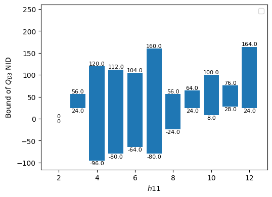
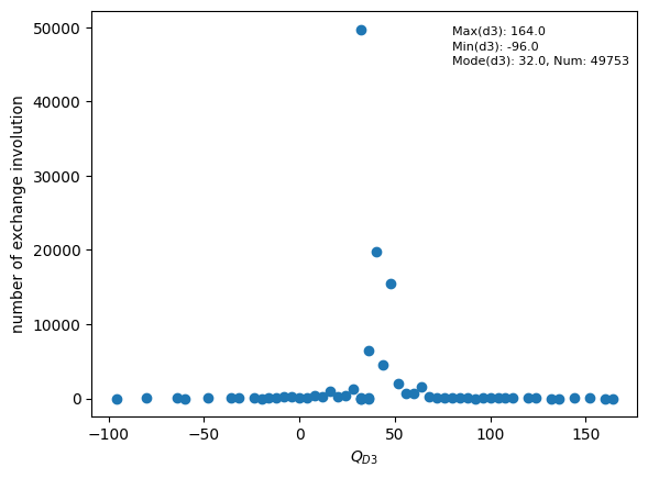
Figure 1: Distribution of $Q_{D3}^{loc}$ under exchange involutions for naive orientifold Type IIB string vacua.

4.1.3 Hodge Number Splitting

Finally, we discuss the decomposition of the Kähler moduli space into odd and even parity equivariant cohomology $H^{1,1}(X/\sigma^{*})=H^{1,1}_{+}(X/\sigma^{*})\oplus H^{1,1}_{-}(X/\sigma^{*})$. The constraint that the Kähler form must be invariant $\sigma^{*}J=J$ ensures that we can always determine the dimension of the even parity space. By deduction, we can then ascertain the dimension of the odd party space $h^{1,1}_{-}(X/\sigma^{*})$, which, as discussed, must be non-trivial in NIDs exchange involutions. The results of this Kähler moduli space splitting are presented in Table 14. The largest $h^{1,1}_{-}$ observed is $3$ for $h^{1,1}(X)\leq 7$ and $6$ for $h^{1,1}(X)\leq 12$. By utilizing the Lefschetz fixed point theorem as indicated in eq.(21), we can further determine the splitting of $h^{2,1}_{\pm}(X/\sigma^{*})$ in the orbifold limit. The value of $h^{2,1}_{\pm}(X/\sigma^{*})$ may be altered by a possible conifold resolution, while $h^{1,1}_{-}(X/\sigma^{*})$ remains robust. In the case of divisor reflection, $h^{1,1}_{-}(X)\equiv 0$ and therefore we do not present the hodge number splitting for this scenario.

Hodge numbers splitting
$\mathbf{h^{1,1}(X)}$		2	3	4	5	6	7	Total
# of Involution		12	61	548	4085	23805	127733	156244
# of $\mathbf{h^{1,1}_{-}}$	1	12	61	495	3683	21019	109175	134445
	2	–	–	53	402	2588	17106	20149
	3	–	–	–	–	198	1452	1650
$\mathbf{h^{1,1}(X)}$		8	9	10	11	12		Total
# of Involution		86	122	82	86	89		465
# of $\mathbf{h^{1,1}_{-}}$	1	48	76	53	49	32		258
	2	22	26	12	18	12		90
	3	14	7	10	6	37		74
	4	2	13	4	13	4		36
	5	–	–	3	–	2		5
	6	–	–	–	–	2		2

Table 14: $h^{1,1}(X/\sigma^{*})$ splitting under the proper divisor exchange involutions

4.2 Reflections

There are two new observations regarding reflection involutions. Firstly, we must verify whether $P_{sym}$ vanishes trivially on the fixed locus $\mathcal{F}_{i}$ and subsequently apply eq.(55) to determine the type of O-plane. Secondly, we identify a new type of free action, as described in Section 3.1.3, which occurs in reflections with more than one divisor.

For each of the triangulation of polytope with $h^{1,1}(X)\leq 6$, we computed all of the single divisor reflections, double divisor reflections and triple divisor reflections. For cases with $h^{1,1}=7$, we computed all single reflections and randomly selected 15 double reflections and 15 triple reflections, as shown in Table.15. For $8\leq h^{1,1}(X)\leq 12$ cases, we compute all single reflections and randomly selected 15 triple reflections, classifying the type of O-plane as presented in Table.16. When considering the D3-tadpole cancelation condition, the naive Orientifold Type IIB string vacua with $O3/O7$ system are compiled in Table.17 and Table.18. It is interesting to note that for single reflections, we obtain the same fixed locus as [36] when restricting to real number solutions.

There are numerous free actions for multi-reflections. Many of them are of the new type, characterized by the absence of a fixed locus in the ambient space $\mathcal{A}$ initially. We denote the previous type of free action as ”type one,” indicating those that do have a fixed locus on $\mathcal{A}$ but do not intersect with the Calabi-Yau manifold $X$.

For the $97,639,633$ naive orientifold Type IIB string vacua with an $O3/O7$-system, the distribution of $Q_{D3}^{loc}$ is shown in Fig. 2. Most involutions result in orientifold Calabi-Yau threefolds with $Q_{D3}^{loc}$ around $136$ in our scan. The smallest and largest $Q_{D3}^{loc}$ are $-192$ and $1008$ respectively. This result aligns with our discussion in [14], where we used the Lefschetz fixed point theorem to demonstrate that the D3-tadpole can be bounded above by $-Q_{3}\leq 252$ for the Kreuzer-Skarke database.

Classification of O-plane fixed point locus
$\mathbf{h^{1,1}(X)}$	2	3	4	5	6	7	Total
Single reflection
# of Reflection	184	3019	39251	488352	5659818	64203360	70393984
O3	2	55	776	10437	100804	760675	872749
O7	64	871	6350	49243	356844	2658260	3071632
O3 and O7	118	2093	32125	428672	5202170	60784425	66449603
Free Action	0	0	0	0	0	0	0
Double divisor reflection
# of Reflection	270	6066	94555	1347475	17653586	70850383	89952335
O5	219	4503	69013	945594	11830587	44782225	57632141
Free Action (type one)	22	515	7481	108385	1428245	5527373 (403)	7072021 (403)
Triple divisors reflection
# of Reflections	418	12328	250141	4332469	65640277	88047584	158283217
O3	96	2413	36515	449416	4335075	3296422	8119937
O7	45	1360	17180	209827	2172172	2113777	4514361
O3 and O7	261	8090	188076	3523818	56670874	78995670	139386789
Free Action (type one)	16	465	8370	149408 (4)	2462156 (395)	3641715 (1008)	6262130 (1407)

Table 15: Classification of O-planes and free actions under reflections for $h^{1,1}\leq 7$

Classification of O-plane fixed point locus
$\mathbf{h^{1,1}(X)}$	8	9	10	11	12	Total
Single reflection
# of Reflection	78930	123420	153858	210130	230431	796769
O3	107	58	21	76	37	299
O7	7663	9732	9112	8650	9074	44231
O3 and O7	71160	113630	144725	201404	221320	752239
Triple divisor reflections
# of Reflection	98067	141432	155496	196174	211884	803053
O3	714	657	249	338	403	2361
O7	4792	5905	4903	4179	4525	24304
O3 and O7	87526	127736	141764	180780	196656	734462
Free Action (type one)	5035 (480)	7134 (1117)	8580 (1499)	10877 (2820)	10300 (2811)	41926    (8727)

Table 16: Classification of O-planes and free actions under reflections for $8\leq h^{1,1}\leq 12$

Naive Orientifold Type IIB String Vacua with $O3/O7$-system
$\mathbf{h^{1,1}(X)}$	2	3	4	5	6	7	Total
Single reflection
# of Reflection	137	2052	24605	275905	2905604	30797733	34006036
O3	0	3	49	771	7403	54261	62487
O7	52	688	4893	35970	257887	1887150	2186640
O3 and O7	85	1361	19663	239164	2640314	28856322	31756909
Triple divisor reflection
# of Reflection	271	6815	125209	1942434	26823480	34289949	63188158
O3	35	762	9142	93922	764601	611384	1479846
O7	42	1088	12592	143910	1406394	1288578	2852604
O3 and O7	178	4500	95105	1555194	22190329	28748272	52593578
Free Action (type one)	16	465	8370	149408 (4)	2462156 (395)	3641715 (1008)	6262130 (1407)

Table 17: Classification of naive orientifold Type IIB string vacua under reflections for $h^{1,1}\leq 7$

Naive Orientifold Type IIB String Vacua with $O3/O7$-system
$\mathbf{h^{1,1}(X)}$	8	9	10	11	12	Total
Single reflection
# of Reflection	25611	36638	43540	56870	67709	230368
O3	0	0	6	0	8	14
O7	3930	4669	5167	4665	5463	23894
O3 and O7	21681	31969	38367	52205	62238	206460
Triple divisor reflection
# of Reflection	29395	38854	40651	49782	56389	215071
O3	455	449	100	71	304	1379
O7	2153	2478	2439	1836	2058	10964
O3 and O7	21752	28793	29532	36998	43727	160802
Free Action (type one)	5035 (480)	7134 (1117)	8580 (1499)	10877 (2820)	10300 (2811)	41926    (8727)

Table 18: Classification of naive orientifold Type IIB string vacua under the reflections for $8\leq h^{1,1}\leq 12$

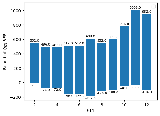
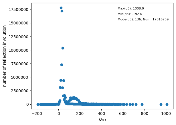
Figure 2: Distribution of $Q_{D3}^{loc}$ under reflections for naive orientifold Type IIB string vacua.

5 Conclusions and Outlook

In this paper, we significantly broaden our scope on orientifold Calabi-Yau threefolds in three key areas. Firstly, we expand the scale of our constructions by three orders of magnitude, increasing from $\mathcal{O}(10^{6})$ to $\mathcal{O}(10^{9})$ orientifold Calabi-Yau threefolds compared to previous work [2]. We extend our construction of orientifold Calabi-Yau threefolds up to $h^{1,1}(X)=12$ in the Calabi-Yau database constructed from the Kreuzer-Skarke list [32]. For $h^{1,1}(X)\leq 7$, we expand our analysis to hypersurfaces in all possible maximal projective crepant partial (MPCP) desingularizations. For $8\leq h^{1,1}(X)\leq 12$, we randomly choose some favorable polytopes for each Hodge number as in  [36]. The number of toric triangulations we analyze increases by one order of magnitude, from $653,062$ [2] to $6,696,714$. We expand our classification to cover both divisor exchange involutions and multi-divisor reflection involutions, which include $156,709$ proper NIDs exchange involutions and $320,229,358$ different types of reflections. Since each of these involutions results in an orientifold Calabi-Yau manifolds, combined those two types of involutions, we constructed a total of $320,386,067$ orientifold Calabi-Yau threefolds in our new database (https://github.com/GroupofXG/anewcydatabase/), which is three orders of magnitude ($\mathcal{O}(10^{3})$) larger than the database in [2], where only exchange involution for small $h^{1,1}(X)$ was considered. We will continue to update our website regularly with new results not included in our current database.

Secondly, we have significantly improved the efficiency of our new algorithm for calculating putative fixed loci under divisor exchanges and reflection involutions. This enhancement enables us to identify the positions of various types of O-planes, which are crucial for D-brane constructions. The upgraded algorithm reduces the calculation complexity required to determine fixed loci by more than five orders of magnitude $\mathcal{O}(10^{5})$ in certain simple examples, even for small values such as$h^{1,1}(X)=7$. We categorize freely acting involutions on Calabi-Yau threefolds into two types: first, those without a fixed locus in the ambient space under the involutions, and second, those with a fixed locus in the ambient space that does not intersect with the Calabi-Yau threefold. In orientifold Calabi-Yau threefolds featuring the $O3/O7$-system, we proceed to classify the so-called “naive orientifold Type IIB string vacua” by considering the D3-tadpole cancellation condition when placing eight $D7$-branes on top of $O7$-plane.

Thirdly, we clarify some ambiguities in the construction of orientifold Calabi-Yau threefolds. One such ambiguity is in determining the type of O-plane using eq.(55). We should be more careful to accurately determine their contribution to the D3-tadpole condition, as described in Section 2.4. Additionally, when solving the $\lambda$ system eq.(31-32) to determine the putative fixed loci, we must ensure that we do not overlook any solutions in the complex $\lambda$ system for $\lambda=e^{i\pi u_{i}}\in\mathbb{C}^{*}$.

The systematic calculations presented in this paper pave the way for extending these analyses beyond our current computational limit into the region $h^{1,1}(X)\geq 12$ of the Kreuzer-Skarke database. Given the extensive size of the orientifold Calabi-Yau database, it is natural to anticipate that in addition to the formal progress, supervised machine learning techniques will be necessary to understand the landscape. In [34], we utilized machine learning technique to classify the polytopes which can result in the orientifold Calabi-Yau with divisor exchange involutions. That study demonstrated that high accuracy could be achieved by training on just 10% of the data for higher $h^{1,1}(X)$. Since we have only calculated part of the polytopes for $8\leq h^{1,1}(X)\leq 12$, it would be great for us to predict the desired polytopes using machine learning techniques on the limited data available and validate these predictions.

In addition to the Kreuzer-Skarke and CICY databases, it has been discovered that relaxing the condition for non-negative entries in the configuration or weighted matrix leads to a new class of Calabi-Yau manifolds, known as “generalized Complete Intersection Calabi-Yau” (gCICYs) [49, 66], along with their toric variations [67, 68]. We have also employed machine learning techniques to generate more gCICY [69]. investigating involutive or more general quotient symmetries of these new manifolds could yield further intriguing insights.

In the context of swampland conjecture, fundamental doubts about the the existence of de-Sitter space have triggered intense discussion. The KKLT scenario [54] has withstood attacks related to the stability of the anti-D3 uplift. Especially, in [70] we asserted that a singular-bulk problem arises because one is forced to glue a large throat into a fairly small Calabi-Yau [71] to get a de-Sitter space. On the other hand, people have explored a landscape of de-Sitter vacua in the large complex structure region of mirror Calabi-Yau manifolds with all order $\alpha^{\prime}$ corrections [17]. Various other corrections, such as warping correction, loop and $\alpha^{\prime}$ correction in the ordinary Type IIB orientifold compactifications was also studied. For example, in the Large Volume Scenario (LVS), considering the warping correction imposes a parameter constraint that provides a lower bound of the number of tadpole that the compactified geoemtry must satisfy [13, 14, 16, 15]. Combined with the tadpole conjecture which gives an upper bound on the number of tadpole [12], this creates a window specifying the types of oreintifold Calabi-Yau compactifications that are feasible. It would be very interesting to investigate the constraints on orientifold Calabi-Yau threefolds imposed by these and other corrections.

Appendix A Fixed locus for reflections of Example A

Table.19 shows the fixed locus we get from the single, double and triple reflections for Example A in Section 3.1.2. The type of O-plane is determined by eq.(55) depending on whether $P_{sym}$ vanish trivially on the fixed sets. These results also collected in Appendix.C.2.2 in the format on the website (https://github.com/GroupofXG/anewcydatabase/). Notice there are three free actions in these reflections we considered.

Reflection	Fixed Locus of O-plane on $X$
$x_{1}$	$[x_{6},x_{7},x_{9}][x_{1}][x_{2}][x_{3}][x_{4}]$
$x_{2}$	$[x_{6},x_{7},x_{9}][x_{2}][x_{1}][x_{3}][x_{4}]$
$x_{3}$	$[x_{6},x_{7},x_{9}][x_{3}][x_{1}][x_{2}][x_{4}]$
$x_{4}$	$[x_{6},x_{7},x_{9}][x_{4}][x_{1}][x_{2}][x_{3}]$
$x_{5}$	$[x_{1},x_{6},x_{7},x_{8}][x_{2},x_{6},x_{9},x_{10}][x_{3},x_{7},x_{9},x_{11}][x_{4},x_{6},x_{7},x_{8}][x_{4},x_{6},x_{9},x_{10}][x_{4},x_{7},x_{9},x_{11}][x_{5}]$
$x_{6}$	$[x_{3},x_{7},x_{9}][x_{1},x_{5},x_{7},x_{8}][x_{2},x_{5},x_{9},x_{10}][x_{4},x_{5},x_{7},x_{8}][x_{4},x_{5},x_{9},x_{10}][x_{6}][x_{5},x_{11}]$
$x_{7}$	$[x_{2},x_{6},x_{9}][x_{1},x_{5},x_{6},x_{8}][x_{3},x_{5},x_{9},x_{11}][x_{4},x_{5},x_{6},x_{8}][x_{4},x_{5},x_{9},x_{11}][x_{7}][x_{5},x_{10}]$
$x_{8}$	$[x_{2},x_{6},x_{10}][x_{3},x_{7},x_{11}][x_{4},x_{6},x_{10}][x_{4},x_{7},x_{11}][x_{1},x_{5},x_{6},x_{7}][x_{8}][x_{5},x_{9}]$
$x_{9}$	$[x_{1},x_{6},x_{7}][x_{2},x_{5},x_{6},x_{10}][x_{3},x_{5},x_{7},x_{11}][x_{4},x_{5},x_{6},x_{10}][x_{4},x_{5},x_{7},x_{11}][x_{9}][x_{5},x_{8}]$
$x_{10}$	$[x_{1},x_{6},x_{8}][x_{3},x_{9},x_{11}][x_{4},x_{6},x_{8}][x_{4},x_{9},x_{11}][x_{2},x_{5},x_{6},x_{9}][x_{10}][x_{5},x_{7}]$
$x_{11}$	$[x_{1},x_{7},x_{8}][x_{2},x_{9},x_{10}][x_{4},x_{7},x_{8}][x_{4},x_{9},x_{10}][x_{3},x_{5},x_{7},x_{9}][x_{11}][x_{5},x_{6}]$
$x_{7}x_{9}$	$[x_{7},x_{9}][x_{1},x_{6}][x_{2},x_{6}][x_{4},x_{6}][x_{3},x_{5},x_{11}][x_{4},x_{5},x_{11}][x_{5},x_{7},x_{8}][x_{5},x_{9},x_{10}]$
$x_{1}x_{2}$	Free Action
$x_{2}x_{6}$	$[x_{2},x_{6}][x_{1},x_{6}][x_{4},x_{6}][x_{7},x_{9}][x_{3},x_{5},x_{11}][x_{4},x_{5},x_{11}][x_{5},x_{7},x_{8}][x_{5},x_{9},x_{10}]$
$x_{3}x_{10}$	$[x_{2},x_{10}][x_{4},x_{10}][x_{6},x_{8}][x_{9},x_{11}][x_{1},x_{5},x_{7}][x_{3},x_{5},x_{7}][x_{4},x_{5},x_{7}][x_{5},x_{6},x_{9}]$
$x_{3}x_{6}$	$[x_{1},x_{6}][x_{2},x_{6}][x_{4},x_{6}][x_{7},x_{9}][x_{3},x_{5},x_{11}][x_{4},x_{5},x_{11}][x_{5},x_{7},x_{8}][x_{5},x_{9},x_{10}]$
$x_{1}x_{3}$	Free Action
$x_{2}x_{5}$	$[x_{2},x_{5}][x_{1},x_{5}][x_{3},x_{5}][x_{4},x_{5}][x_{6},x_{7},x_{8}][x_{6},x_{9},x_{10}][x_{7},x_{9},x_{11}]$
$x_{1}x_{7}$	$[x_{1},x_{7}][x_{3},x_{7}][x_{4},x_{7}][x_{6},x_{9}][x_{2},x_{5},x_{10}][x_{4},x_{5},x_{10}][x_{5},x_{6},x_{8}][x_{5},x_{9},x_{11}]$
$x_{6}x_{7}$	$[x_{6},x_{7}][x_{2},x_{9}][x_{3},x_{9}][x_{4},x_{9}][x_{5},x_{10}][x_{1},x_{5},x_{8}][x_{4},x_{5},x_{8}][x_{5},x_{7},x_{11}]$
$x_{5}x_{10}$	$[x_{5},x_{10}][x_{2},x_{6},x_{9}][x_{4},x_{6},x_{9}][x_{7}]$
$x_{1}x_{5}$	$[x_{1},x_{5}][x_{2},x_{5}][x_{3},x_{5}][x_{4},x_{5}][x_{6},x_{7},x_{8}][x_{6},x_{9},x_{10}][x_{7},x_{9},x_{11}]$
$x_{5}x_{6}$	$[x_{5},x_{6}][x_{1},x_{7},x_{8}][x_{2},x_{9},x_{10}][x_{4},x_{7},x_{8}][x_{4},x_{9},x_{10}][x_{11}]$
$x_{3}x_{5}$	$[x_{3},x_{5}][x_{1},x_{5}][x_{2},x_{5}][x_{4},x_{5}][x_{6},x_{7},x_{8}][x_{6},x_{9},x_{10}][x_{7},x_{9},x_{11}]$
$x_{1}x_{8}$	$[x_{1},x_{8}][x_{4},x_{8}][x_{6},x_{10}][x_{7},x_{11}][x_{2},x_{5},x_{9}][x_{3},x_{5},x_{9}][x_{4},x_{5},x_{9}][x_{5},x_{6},x_{7}]$
$x_{2}x_{7}$	$[x_{1},x_{7}][x_{3},x_{7}][x_{4},x_{7}][x_{6},x_{9}][x_{2},x_{5},x_{10}][x_{4},x_{5},x_{10}][x_{5},x_{6},x_{8}][x_{5},x_{9},x_{11}]$
$x_{4}x_{5}x_{6}$	$[x_{1},x_{5},x_{6}][x_{2},x_{5},x_{6}][x_{3},x_{11}][x_{4},x_{11}][x_{7},x_{8}][x_{9},x_{10}]$
$x_{3}x_{8}x_{9}$	$[x_{5},x_{6},x_{7},x_{9}][x_{1},x_{5}][x_{2},x_{5}][x_{3},x_{5}][x_{4},x_{5}]$
$x_{4}x_{7}x_{11}$	$[x_{4},x_{7},x_{11}][x_{2},x_{6},x_{10}][x_{3},x_{7},x_{11}][x_{4},x_{6},x_{10}][x_{1},x_{5},x_{6},x_{7}][x_{8}][x_{5},x_{9}]$
$x_{1}x_{6}x_{7}$	$[x_{1},x_{6},x_{7}][x_{2},x_{5},x_{6},x_{10}][x_{3},x_{5},x_{7},x_{11}][x_{4},x_{5},x_{6},x_{10}][x_{4},x_{5},x_{7},x_{11}][x_{9}][x_{5},x_{8}]$
$x_{5}x_{7}x_{11}$	$[x_{1},x_{5},x_{8}][x_{4},x_{5},x_{8}][x_{2},x_{9}][x_{3},x_{9}][x_{4},x_{9}][x_{6},x_{7}]$
$x_{2}x_{7}x_{11}$	$[x_{2},x_{6},x_{10}][x_{3},x_{7},x_{11}][x_{4},x_{6},x_{10}][x_{4},x_{7},x_{11}][x_{1},x_{5},x_{6},x_{7}][x_{8}][x_{5},x_{9}]$
$x_{5}x_{6}x_{10}$	$[x_{1},x_{5},x_{8}][x_{4},x_{5},x_{8}][x_{2},x_{9}][x_{3},x_{9}][x_{4},x_{9}][x_{6},x_{7}]$
$x_{2}x_{5}x_{8}$	$[x_{1},x_{5},x_{8}][x_{4},x_{5},x_{8}][x_{2},x_{9}][x_{3},x_{9}][x_{4},x_{9}][x_{6},x_{7}]$
$x_{1}x_{9}x_{11}$	$[x_{1},x_{6},x_{8}][x_{3},x_{9},x_{11}][x_{4},x_{6},x_{8}][x_{4},x_{9},x_{11}][x_{2},x_{5},x_{6},x_{9}][x_{10}][x_{5},x_{7}]$
$x_{5}x_{8}x_{9}$	Free Action
$x_{1}x_{5}x_{9}$	$[x_{2},x_{5},x_{9}][x_{3},x_{5},x_{9}][x_{1},x_{8}][x_{4},x_{8}][x_{6},x_{10}][x_{7},x_{11}]$
$x_{3}x_{6}x_{8}$	$[x_{1},x_{6},x_{8}][x_{3},x_{9},x_{11}][x_{4},x_{6},x_{8}][x_{4},x_{9},x_{11}][x_{2},x_{5},x_{6},x_{9}][x_{10}][x_{5},x_{7}]$
$x_{1}x_{5}x_{7}$	$[x_{1},x_{5},x_{7}][x_{3},x_{5},x_{7}][x_{2},x_{10}][x_{4},x_{10}][x_{6},x_{8}][x_{9},x_{11}]$
$x_{2}x_{4}x_{6}$	$[x_{3},x_{7},x_{9}][x_{1},x_{5},x_{7},x_{8}][x_{2},x_{5},x_{9},x_{10}][x_{4},x_{5},x_{7},x_{8}][x_{4},x_{5},x_{9},x_{10}][x_{6}][x_{5},x_{11}]$
$x_{4}x_{6}x_{7}$	$[x_{1},x_{6},x_{7}][x_{2},x_{5},x_{6},x_{10}][x_{3},x_{5},x_{7},x_{11}][x_{4},x_{5},x_{6},x_{10}][x_{4},x_{5},x_{7},x_{11}][x_{9}][x_{5},x_{8}]$

Table 19: Fixed locus under the reflections for the Example A in Section 3.1.2.

Appendix B Pseudocode description of new algorithm

Here we present the pseudo-code for the new algorithm to find the putative fixed locus (Algorithm.1) and the optimized logical to reduce the possible fixed locus needed to test (Algorithm.2).

$m=W.rows$

$n=\mathcal{F}.length$

let $M$ be a matrix of size $m\times n$

for $i\leftarrow 0$ to $n$ do

       set column $i$ of $M$ to be the toric weight vector of $\mathcal{F}[i]$

      

let $b$ be an array of zeros of size $n$

for $i\leftarrow 0$ to $n$ do

       if $\mathcal{F}[i]\in\mathcal{G}_{-}$ then

             $b[i]=1$

            

      

/* Improvement */

let $u_{iT}=2^{m}$

let $u_{i}=0$

while $u_{i}<u_{iT}$ do

       let $odd=false$

       let $u\_real_{i}$ be the $n$ bit binary type of $u_{i}$

       /* for $u_{i}=3$ and $n=5$, $u\_real_{i}=00011$, the i-th bit tells the value of $\mathcal{F}_{i}$ */

       for $x\leftarrow 0$ to $n$ do

             $col=M[x]$

             let $value_{x}=\sum_{i\in\text{range}(m)}(u\_real_{i}[i]\cdot\text{col}[i])+b[x]$

             if $value_{x}\%2=1$ then

                   $odd=True$

                   break

            

      if not $odd$ then

             return true

      $u_{i}+=1$

return false

Algorithm 1 $\textrm{WEIGHT\_FIXED\_REALSPACE}(\mathcal{F},W,\mathcal{G}_{0},\mathcal{G}_{+},\mathcal{G}_{-})$

$\mathcal{G}=\mathcal{G}_{0}\cup\mathcal{G}_{+}\cup\mathcal{G}_{-}$

let $\mathcal{L}_{f}$ be list of fixed points computed before in real space

let $\mathcal{L}_{fs}$ be a sum of SR ideal and $\mathcal{L}_{f}$

let $\mathcal{L}_{uf}$ be an empty list

let $\mathcal{S}$ be the power set of $\mathcal{G}$

/* $\mathcal{S}$ are sorted so the number of divisor of element start large which means small in geometry */

for $\mathcal{F}\in\mathcal{S}$ do

       skip = false

       for $\mathcal{T}\in\mathcal{L}_{uf}$ do

             if $\mathcal{F}\subset\mathcal{T}$ then

                   /* Non-fixed locus $\mathcal{T}$ is a part of $\mathcal{F}$ in geometry, so $\mathcal{F}$ can not fixed */

                   skip = true

                   break

            

      if skip then

             continue

      for $\mathcal{T}\in\mathcal{L}_{fs}$ do

             if $\mathcal{T}\subset\mathcal{F}$ then

                   /* $\mathcal{F}$ is a part of $\mathcal{T}$ in geometry, so $\mathcal{F}$ is ruled out by existing fixed point or singularity introduced by SR ideal */

                   skip = true

                   break

            

      if skip then

             continue

      if not $\textrm{CONSISTENT}(\mathcal{F},\mathcal{G}_{0},\mathcal{G}_{+},\mathcal{G}_{-})$ then

             continue

            

      if not $\textrm{WEIGHT\_FIXED}(\mathcal{F},W,\mathcal{G}_{0},\mathcal{G}_{+},\mathcal{G}_{-})$ then

             /* This WEIGHT_FIXED algorithm is just the old one in complex space */

             append $\mathcal{F}$ to $\mathcal{L}_{uf}$

             continue

      append $\mathcal{F}$ to $\mathcal{L}_{f}$

       append $\mathcal{F}$ to $\mathcal{L}_{fs}$

      

return $\mathcal{L}_{f}$

Algorithm 2 $\textrm{FIXED\_LOCI\_WEIGHTS\_NEW}(W,SR\ ideal,\mathcal{G}_{0},\mathcal{G}_{+},\mathcal{G}_{-})$

Appendix C Database Format

C.1 Terminology

The entry for each involution will contain the following terminologes :

C.1.1 Divisor exchange involutions

• Polyid: The index numbers labeling the polytope in the database.

• Tri_id: The index of triangulation in a given polytope.

• BP_not_in_F: Boundary points not interior to facets of a polytope, corresponding to the vertex in the dual-polytope $\Delta^{*}$ of the toric ambient space.

• F_Intsec: Quartet intersection number on the ambient space $\mathcal{A}$.

• triple_inters: Triple intersection number on the Calabi-Yau threefolds $X$.

• INVOL: The involution considered in this example.

• KK_data: The geometric data of this polytope mentioned in Kreuzer-Skarke database.

• Linear_I: Linear ideal of the polytope.

• OPLANES: The locus and type of O-plane, followed by their contribution to D3-tadpole locally labeled as “value”.

              { type of O-plane: [[Fixed Locus_1], number of O-plane_1,...]
                ...
                "tadpole_cancel": True or False,
                "value": contribution to D3-tadpole
                "[h12p,h12n,smooth]" :  [h21+, h21-, whether P_sym is smooth]
               }
                  
  

• P_symm1: The polynomail expression of invariant hypersurface under the involution.

• Polys: Generators of $\mathcal{G}$ for exchange involutions.

• Q_parity: The parity of the holomorhpic three form under involution.

• Q_str: The expression of Q.

• SR_list: The Stanley-Reisner ideal.

• Sectors: Different patches of the polytope associated to the SR-ideal.

• Wmatrix2: GLSM weighted matrix $\mathbf{W}$ together with the degree of hypersurface.

• divisor_indenp: Independent divisors chosen to be the basis of divisor class.

• divisors_Hodge: The Hodge numbers of each divisors.

• Hodge_split_p_n: The value of $[h^{1,1}_{+},h^{1,1}_{-}]$.

• rwmat_for_y_notreduced: The new weight matrix $\tilde{\mathbf{W}}$ after Segre embedding.

C.1.2 Reflections

The terminologes for reflections are almost the same as divisor exchange involution, except the single, double and triple reflections are labeled as invol1, invol2 and invol3. The new type of free action described in Section 2.5 for multi-reflections are labeled as “total fixed”. The format is as follows:

[Reflection]: type of O-plane, contribution to D3-tadpole, Fixed Locus

• invol1: Type of O-plane, its contribution to D3-tadpole and the fixed locus for single reflection.

• invol2: Type of O-plane, its contribution to D3-tadpole and the fixed locus for double reflection.

• invol3: Type of O-plane, its contribution to D3-tadpole and the fixed locus for triple reflection.

C.2 Entry for Example A

C.2.1 Divisor exchange involution

• polyid: 545

• tri_id: 5

• BP_not_in_F:

  [
  [-2, -3, -2, -2], [0, 1, 0, 0], [0, 1, 0, 2], [0, 1, 2, 0],
  [1, 0, 0, 0], [-1, -1, -1, -1], [-1, -1, -1, 0], [-1, -1, 0, -1],
  [0, 1, 0, 1], [0, 1, 1, 0], [0, 1, 1, 1]
  ]
  

• F_Intsec:

  [
  [[[2, 0, 0, 0, 0, 0, 0], [0, -2, 0, 0, 0, 0, 0], [0, 0, -2, 0, 0, 0, 0],
  [0, 0, 0, -2, 0, 0, 0], [0, 0, 0, 0, -2, 0, 0], [0, 0, 0, 0, 0, -2, 0],
  [0, 0, 0, 0, 0, 0, -2]],..., [[-2, 0, -2, 0, -2, 0, 0],
  [0, 0, 0, 0, 0, 0, 0], [-2, 0, -2, 0, -2, 0, 0], [0, 0, 0, 0, 0, 0, 0],
  [-2, 0, -2, 0, -2, 0, 0], [0, 0, 0, 0, 0, 0, 0], [0, 0, 0, 0, 0, 0, -2]]]
  ]
  

• triple_inters:

  {(1, 5, 7): 3, (1, 6, 7): 3, (1, 5, 6): 3, (1, 5, 8): 3, (1, 6, 8): 3,
  ...
  , (0, 0, 5): 54, (0, 0, 2): 27, (0, 0, 3): 27, (0, 0, 4): 27, (0, 0, 0): 162}
  

• INVOL:

  [[7, 9], [6, 8], [0, 1]]
  

• KK_data:

  4 5  M:12 5 N:40 5 H:37,7 [60]
          
  

• Linear_I:

  ["1/2*z5 - 1/2*z6 - 1/2*z7 - 1/2*z8",
  "1/2*z5 - 1/2*z6 - 1/2*z9 - 1/2*z10",
  "1/2*z5 - 1/2*z7 - 1/2*z9 - 1/2*z11",
  "1/2*z5 - 1/2*z8 - 1/2*z10 - 1/2*z11",
  "z5",
  "z6",
  "z7",
  "z8",
  "z9",
  "z10",
  "z11"]
          
  

• OPLANES:

  {
    "O3": [
      [
        "[x3, x4, x10]",
        3.0
      ],
      [
        "[x2, x4, x10]",
        3.0
      ],
      [
        "[x3, x5, x0^2*x6*x7 + x1^2*x8*x9]",
        3.0
      ]
    ],
    "O7": [
      [
        "[x0^2*x6*x7 - x1^2*x8*x9]",
        1
      ]
    ],
    "tadpole_cancel": true,
    "value": 36.0,
    "[h12p, h12n, smooth]": "[12.0, 25.0, True]"
  }
          
  

• P_symm1:

  x0^6*x5^3*x6^3*x7^3 + x0^4*x1^2*x5^3*x6^2*x7^2*x8*x9 +
  x0^2*x1^4*x5^3*x6*x7*x8^2*x9^2 + x1^6*x5^3*x8^3*x9^3 +
  ...
  + x2^2*x4^2*x6*x8*x10 + x3^2*x4^2*x7*x9*x10 + x4^3
          
  

• Polys:

  [x7*x9, x6*x8, x0*x1, x0^2*x6*x7 + x1^2*x8*x9, x0^2*x6*x7 - x1^2*x8*x9]
          
  

• Q_parity: -1

• Q_str:
  

  +(1 z1z2z3z4z5z6z7 dz8dz9dz10dz11) +(1 z1z2z3z4z5z6z8 dz7dz9dz10dz11)
  -(1 z1z2z3z4z5z6z9 dz7dz8dz10dz11) -(1 z1z2z3z4z5z6z10 dz7dz8dz9dz11)
  ...
  +(4 z4z6z7z8z9z10z11 dz1dz2dz3dz5) -(8 z5z6z7z8z9z10z11 dz1dz2dz3dz4)
          
  

• SR_list:

  [
  [z1, z2], [z1, z3], [z1, z4], [z1, z9], [z1, z10], [z1, z11], [z2, z3],
  [z2, z4], [z2, z7], [z2, z8], [z2, z11], [z3, z4], [z3, z8], [z3, z10],
  [z4, z5, z6, z7], [z4, z5, z6, z9], [z5, z6, z7, z8], [z5, z6, z9, z10],
  [z5, z6, z11], [z7, z9], [z7, z10], [z8, z9], [z8, z10], [z8, z11], [z10, z11]
  ]
          
  

• Sectors:

  [
  [x0 - 1, x1 - 1, x2 - 1, x3 - 1, x7 - 1, x9 - 1, x10 - 1],
  [x0 - 1, x1 - 1, x2 - 1, x4 - 1, x5 - 1, x7 - 1, x9 - 1],
  [x0 - 1, x1 - 1, x2 - 1, x4 - 1, x6 - 1, x7 - 1, x10 - 1],
  ...
  [x1 - 1, x2 - 1, x3 - 1, x5 - 1, x8 - 1, x9 - 1, x10 - 1],
  [x1 - 1, x2 - 1, x3 - 1, x6 - 1, x8 - 1, x9 - 1, x10 - 1],
  [x1 - 1, x2 - 1, x3 - 1, x7 - 1, x8 - 1, x9 - 1, x10 - 1]
  ]
          
  

• Wmatrix2:

  [
  [-6  1 -1  0  0  2  0  0  0  2  2  0]
  [ 0  0  1  1  0  0  0  0  0 -2  0  0]
  [ 0  0  1  0  1  0  0  0  0  0 -2  0]
  [-3  0 -1  0  0  1  1  0  0  1  1  0]
  [-3  0  0  0  0  1  0  1  0  0  1  0]
  [-3  0  0  0  0  1  0  0  1  1  0  0]
  [ 0  0  1  0  0  0  0  0  0 -1 -1  1]
  ]
          
  

• divisor_indenp:

  [’z5’, ’z6’, ’z7’, ’z8’, ’z9’, ’z10’, ’z11’]
  

• divisors_Hodge:

  [
  ’[1, 0, 0, 7]’, ’[1, 0, 0, 7]’, ’[1, 0, 0, 7]’, ’[1, 0, 0, 16]’,
  ’[1, 0, 4, 44]’, ’[1, 1, 0, 11]’, ’[1, 1, 0, 11]’, ’[1, 1, 0, 2]’,
  ’[1, 1, 0, 11]’, ’[1, 1, 0, 2]’, ’[1, 1, 0, 2]’
  ]
  

• Hodge_split_p_n:

  [5, 2]
  

• rwmat_for_y_notreduced:

  [
  [ 2  0  1  0  2  0  1  2  2  0]
  [ 0 -2  1  0  0  0  1  0  0  0]
  [-2  2 -1  1  0  0  0  0  0  0]
  [ 1 -1  1  0  1  1  0  0  0  0]
  [ 1  1  0  0  1  0  0  1  1  0]
  [ 1  1  0  0  1  0  0  1  1  0]
  [-1  1 -1  0  0  0  0  0  0  1]
  ]
          
  

C.2.2 Reflection

• invol1:

      [0]: O3: 3 [x5, x6, x8], O7: 9 [x0], O7: 9 [x1], O7: 9 [x2], O7: 18 [x3]
      [1]: O3: 3 [x5, x6, x8], O7: 9 [x1], O7: [x0], O7: 9 [x2], O7: 18 [x3]
      ...
      [10]: O3: 3 [x0, x6, x7], O3: 3 [x1, x8, x9], O3: 3 [x3, x6, x7],
            O3: 3 [x3, x8, x9], O3: 1 [x2, x4, x6, x8], O7: 7 [x4, x5]
                
  

• invol2:

      [6, 8]: O5: [x6, x8], O5: [x0, x5], O5: [x1, x5], O5: [x3, x5], O5: [x2, x4, x10],
              O5: [x3, x4, x10], O5: [x4, x6, x7], O5: [x4, x8, x9]
      [0, 1]: [[x0], [x1], [x2], [x3], [x4], [x5], [x6], [x7], [x8], [x9], [x10]] total fixed
      ...
      [1, 6]: O5: [x0, x6], O5: [x2, x6], O5: [x3, x6], O5: [x5, x8], O5: [x1, x4, x9],
              O5: [x3, x4, x9], O5: [x4, x5, x7], O5: [x4, x8, x10]
            
  

• invol3:

      [3, 4, 5]: O3: 3 [x0, x4, x5], O3: 3 [x1, x4, x5], O7: 3 [x2, x10],
                 O7: 3 [x3, x10], O7: 4 [x6, x7], O7: 4 [x8, x9]
      [2, 7, 8]: O3: 1 [x4, x5, x6, x8], O7: 3 [x0, x4], O7: 3 [x1, x4],
                 O7: 3 [x2, x4], O7: 6 [x3, x4]
      ...
      [0, 4, 6]: O3: 3 [x0, x4, x6], O3: 3 [x2, x4, x6], O7: 3 [x1, x9],
                 O7: 3 [x3, x9], O7: 4 [x5, x7], O7: 4 [x8, x10]