Diffusion Models for Tabular Data Imputation and Synthetic Data Generation

Abstract.

Data imputation and data generation have important applications for many domains, like healthcare and finance, where incomplete or missing data can hinder accurate analysis and decision-making. Diffusion models have emerged as powerful generative models capable of capturing complex data distributions across various data modalities such as image, audio, and time series data. Recently, they have been also adapted to generate tabular data. In this paper, we propose a diffusion model for tabular data that introduces three key enhancements: (1) a conditioning attention mechanism, (2) an encoder-decoder transformer as the denoising network, and (3) dynamic masking. The conditioning attention mechanism is designed to improve the model’s ability to capture the relationship between the condition and synthetic data. The transformer layers help model interactions within the condition (encoder) or synthetic data (decoder), while dynamic masking enables our model to efficiently handle both missing data imputation and synthetic data generation tasks within a unified framework. We conduct a comprehensive evaluation by comparing the performance of diffusion models with transformer conditioning against state-of-the-art techniques, such as Variational Autoencoders, Generative Adversarial Networks and Diffusion Models, on benchmark datasets. Our evaluation focuses on the assessment of the generated samples with respect to three important criteria, namely: (1) Machine Learning efficiency, (2) statistical similarity, and (3) privacy risk mitigation. For the task of data imputation, we consider the efficiency of the generated samples across different levels of missing features.

1. Introduction

The exponential increase in data generation across sectors such as healthcare, finance, telecommunications, and energy has significantly enhanced decision-making capabilities powered by Artificial Intelligence (AI) and Machine Learning (ML) technologies. However, the presence of missing or incomplete data poses significant challenges, undermining the reliability of analyses derived from ML algorithms. Moreover, the rise in strict AI regulations and data protection laws has intensified the need for robust data privacy measures, challenging traditional data handling practices.

Centralised, cloud-based ML solutions, while efficient in terms of model performance, have been repeatedly criticised for their inherent data privacy issues. Specifically, the centralised nature of these solutions necessitates the transfer of large volumes of multidimensional and privacy-sensitive user data, which raises significant privacy concerns. Moreover, centralised models contend with the issue of single point failure. Even advanced solutions like Federated Learning (FL), which aim to decentralize data processing to enhance privacy, depend on a central server for coordinating training processes and aggregating updates. This centralization leaves systems vulnerable to potential privacy risks from information leakage attacks [37, 17], which can infer private data from shared model updates.

In addition, these ML models are particularly prone to utility loss due to missing or corrupted data, especially when dealing with sparse datasets. The handling of missing data can favour certain statistical interpretations, and subsequent implications for policy and practice [9]. For instance, the mean substitution method, often used to handle missing data, may lead to inconsistent bias, especially in the presence of a great inequality in the number of missing values for different features [26]. Furthermore, when missing data are not missing at random (MNAR), even multiple imputations do not lead to valid results [16]. Such imputation methods that fill in blanks with estimated values may inadvertently lead to the creation and transmission of inaccurate or misleading information.

Current efforts to address these issues, such as the application of differential privacy or the use of specialised hardware (e.g., Trusted Execution Environments [36]), often result in a trade-off between privacy and data utility or necessitate additional infrastructure.

Given these challenges, there is a pressing need for solutions that effectively manage data integrity and privacy. Recent advancements in machine learning, specifically Generative Adversarial Networks (GANs) [15] and Diffusion Models [46, 18], have shown promise in generating high-fidelity synthetic data that preserve the statistical properties of original datasets while mitigating privacy concerns, since they follow the original distribution without directly exposing or replicating sensitive information. These generative methods have found their way into applications like image and audio processing [61, 44, 34] and, more recently, have expanded to address tabular data as well [59, 30, 29, 32, 62].

Specifically, for tabular data, synthetic data stands out as a privacy-preserving alternative to real data that may contain personally identifiable information. It enables the generation of datasets that mimic the statistical properties of their original counterparts, while mitigating the risk of individual privacy breaches. In addition, this approach to generating new samples can augment existing datasets by, for example, correcting class imbalances, reducing biases, or expanding their size when dealing with sparse or limited data. Furthermore, integrating methods for differential privacy [11, 22] with generative models for tabular data makes possible to share synthetic datasets across units in large organizations, addressing legal or privacy concerns that often impede technological innovation adoption.

In this study, we consider synthetic data generation as a general case of data imputation. In instances where every column in a sample has missing values, the task of data imputation naturally transitions to synthesizing new data. We introduce MTabGen, a new conditioning in diffusion model for tabular data using an encoder-decoder transformer and a dynamic masking mechanism that makes it possible to tackle both tasks with a single model. During the training step of the model, the dynamic masking randomly masks features that we later generate or impute. The unmasked features are used as context or condition for the reconstruction of masked features during the reverse denoising phase of the diffusion process. We refer to the features to be denoised during the reverse denoising phase as masked features hereinafter.

In our analysis, we perform a rigorous evaluation of the proposed approach using several benchmark datasets, each with a wide range of features. We demonstrate that our method consistently outperforms existing baselines, particularly in handling high-dimensional datasets, thereby highlighting its robustness and adaptability in complex tabular data scenarios. The key contributions of this work are the following:

• We propose a new conditioning mechanism for tabular diffusion models. We model the interaction between condition and masked features (e.g., features to-be-denoised) by using an attention mechanism. Within this mechanism, the embedding of the masked features plays the role of query (Q), and the embedding of the condition plays the roles of key (K) and value (V) (see [54] for details). Compared to the standard approach, where condition and masked features are added [65, 30] or concatenated [32], our method allows to learn more complex relationships showing globally improved performances.

• We incorporate a full encoder-decoder transformer within the diffusion process as the denoising model. The encoder learns the condition embedding, while the decoder models the representation of the masked features. Using transformer layers enhances the learning of inter-feature interactions: within the condition for the encoder and the masked features for the decoder. Additionally, the encoder-decoder architecture allows the implementation of the conditioning attention mechanism explained in the previous item. To the best of our knowledge, [65] is the only prior work that has considered diffusion models for tabular data, using a transformer denoising component. However, in this paper, the transformer layer is limited to learning the masked feature representation, without modeling the condition nor using conditioning attention mechanism.

• We extend the masking mechanism proposed by Zheng and Charoenphakdee [65] to train a single model capable of multitasking, handling both missing data imputation and synthetic data generation. This is facilitated by the transformer encoder-decoder architecture, which allows for arbitrary modification of the split between condition and masked features during the training phase.

• We conduct extensive experiments on several public datasets and demonstrate substantial performance gains over state-of-the-art baselines, for both tasks, missing data imputation and synthetic data generation. We evaluate the synthetic data with respect to three important criteria: (1) ML efficiency, (2) statistical similarity and (3) privacy risk.

2. Related work

Diffusion Models. Originally introduced by Sohl-Dickstein et al. [46] and Ho et al. [18], diffusion models utilize a two-step generative approach. Initially, they degrade a data distribution using a forward diffusion process by continuously introducing noise from a known distribution. Subsequently, they employ a reverse process to reconstruct the original data structure. At their core, these models leverage parameterized Markov chains, starting typically from a foundational distribution such as a standard Gaussian, and use deep neural networks to reverse the diffusion. Demonstrated by recent advancements [38, 10], diffusion models have showcased their capability, potentially surpassing GANs in image generation capabilities. Recent works, such as StaSy [29], CoDi [32], Tabsyn [62], TabDDPM [30] or TabCSDI [65], adapt diffusion models to handle tabular data in both synthetic data generation and data imputation tasks.

Missing Data Imputation. Handling missing values in datasets is a non-trivial problem. Traditional approaches may involve excluding rows or columns with missing entries or imputing missing values using the average values of the corresponding feature. However, recent efforts have been focusing on ML techniques [53, 5, 23] and deep generative models [60, 6, 57, 20, 31], and new models using diffusion processes have been developed for data imputation tasks. Specifically, TabCSDI, based on the CSDI model originally designed for time-series data, adapts this technology for tabular data imputation. TabCSDI employs three common preprocessing techniques: (1) one-hot encoding, (2) analog bits encoding, and (3) feature tokenization. These methods allow it to treat continuous and categorical variables uniformly in a Gaussian diffusion process, regardless of their original types. In contrast, MTabGen implements a dual diffusion mechanism adapted for both continuous and categorical data, maintaining the unique statistical properties of each feature type throughout the diffusion process. As noted previously, TabCSDI uses a transformer layer to learn only the interactions within the masked features and then adds the transformer output to the condition embedding. In our case, MTabGen uses a more adaptable and general approach: the condition embedding is modeled by using a transformer encoder and then fed into a conditioning attention mechanism.

Generative models. The application of this family of models to tabular data has been gaining increased attention within the ML community [59, 12, 24, 13, 50, 64, 28, 63, 39, 58]. In particular, tabular VAEs [59] and GANs [59, 12, 24, 13, 50, 64, 28, 63, 39, 58] have shown promising results. Recently, StaSy [29], CoDi [32], Tabsyn [62], TabDDPM [30] have been proposed as powerful alternatives to tabular data generation, leveraging the strengths of Diffusion Models. Specifically, STaSy, applies a score-based generative approach [47], integrating self-paced learning and fine-tuning strategies to enhance data diversity and quality by stabilizing the denoising score matching training process. CoDi addresses training challenges with mixed-data types using a dual diffusion model approach. One model handles continuous features and the other manages discrete (categorical) features. Both models use a UNet-based architecture with linear layers instead of traditional convolutional layers, and are trained to condition on each other’s outputs. This fixed conditioning setup is designed specifically to handle the interactions between continuous and categorical variables effectively. Tabsyn applies the concepts of latent diffusion models [45, 52] to tabular data. First, a VAE encodes mixed-type data into a continuous latent space and then a diffusion model learns this latent distribution. The VAE uses a transformer encoder-decoder to capture feature relationships, while the diffusion model uses an MLP in the reverse denoising process. There are no transformers used in the denoising step, and it does not include a mask conditional method. Finally, TabDDPM manages datasets with mixed data types by using Gaussian diffusion for continuous features and multinomial diffusion for categorical ones. In the preprocessing step, continuous features are scaled using a min-max scaler, and categorical features are one-hot encoded. Then each type of data is sent to its specific diffusion process. After the denoising process, the preprocessing is reversed by scaling back continuous variables, and categorical ones are estimated by first applying a softmax function and then selecting the most likely category. For classification datasets, TabDDPM adopts a class-conditional model consisting in the addition of the condition embedding to the output of the model, while for regression datasets, it integrates target values as an additional feature. It utilizes an MLP architecture as the denosing network optimized with a hybrid objective function that includes mean squared error and KL divergence to predict continuous and categorical data.

Our method is based on TabDDPM, following the same logic of having two separate diffusion models for continuous and categorical data. To this end, we augment the model with three key improvements. First, we employ a transformer-based encoder-decoder as the denoising model, which enhances the capability to learn inter-feature interactions for both, condition and masked features. Second, we integrate the conditioning directly into the transformer’s attention mechanism rather than simply adding embeddings: this approach reduces learning bias, improving how the interaction between the condition and masked features is modeled. Third, we enable dynamic masking during training, which allows our model to handle varying numbers of visible variables, thus supporting both synthetic data generation and missing data imputation within a single framework. In the following sections, we demonstrate that these contributions lead to improved results across various datasets, outperforming TabDDPM and other state-of-the-art algorithms.

3. Background

Diffusion models, as introduced by Sohl-Dickstein et al. [46] and Ho et al. [18], involve a two-step process: first degrading a data distribution using a forward diffusion process and then restoring its structure through a reverse process. Drawing insights from non-equilibrium statistical physics, these models employ a forward Markov process which converts a complex unknown data distribution into a simple known distribution (e.g., Gaussian) and vice-versa a generative reverse Markov process that gradually transforms a simple known distribution into a complex data distribution.

More formally, the forward Markov process $q\left(x_{1:T}\middle|x_{0}\right){=}\prod_{t=1}^{T}q\left(x_{t}\middle|x_{t-1}\right)$ gradually adds noise to an initial sample $x_{0}$ from the data distribution $q\left(x_{0}\right)$ sampling noise from the predefined distributions $q\left(x_{t}\middle|x_{t-1}\right)$ with variances $\left\{\beta_{1},\dots,\beta_{T}\right\}$. Here $t\,\in\left[1,T\right]$ is the timestep, $T$ is the total number of timesteps used in the forward/reverse diffusion processes and $1:T$ means the range of timesteps from $t=1$ to $t=T$.

The reverse diffusion process $p\left(x_{0:T}\right){=}\prod_{t=1}^{T}p\left(x_{t-1}\middle|x_{t}\right)$ gradually denoises a latent variable $x_{T}{\sim}q\left(x_{T}\right)$ and allows generating new synthetic data. Distributions $p\left(x_{t-1}\middle|x_{t}\right)$ are approximated by a neural network with parameters $\theta$. The parameters are learned optimizing a variational lower bound (VLB):

(1) $$L_{\text{vlb}} :=L_{0}+L_{1}+...+L_{T-1}+L_{T}$$

(2) $$L_{0} :=-\log p_{\theta}(x_{0}|x_{1})$$

(3) $$L_{T-1} :=D_{KL}(q(x_{T-1}|x_{T},x_{0})\;||\;p_{\theta}(x_{T-1}|x_{T}))$$

(4) $$L_{T} :=D_{KL}(q(x_{T}|x_{0})\;||\;p(x_{T}))$$

The term $q\left(x_{T-1}\middle|x_{T},x_{0}\right)$ is the forward process posterior distribution conditioned on $x_{T}$ and on the initial sample $x_{0}$. $L_{T-1}$ is the Kullback-Leibler divergence between the posterior of the forward process and the parameterized reverse diffusion process $p_{\theta}\left(x_{T-1}\middle|x_{T}\right)$.

Gaussian diffusion models operate in continuous spaces $\left(x_{t}\in\mathbb{R}^{n}\right)$ and in this case the aim of the forward Markov process is to convert the complex unknown data distribution into a known Gaussian distribution. This is achieved by defining a forward noising process $q$ that given a data distribution $x_{0}\sim q(x_{0})$, produces latents $x_{1}$ through $x_{T}$ by adding Gaussian noise at time $t$ with variance $\beta_{t}\in(0,1)$.

(5) $$\begin{gathered}q\left(x_{t}\middle|x_{t-1}\right):=\mathcal{N}\left(x_{t};\sqrt{1-\beta_{t}}x_{t-1},\beta_{t}I\right)\\ q\left(x_{T}\right):=\mathcal{N}\left(x_{T};0,I\right)\\ \end{gathered}$$

If we know the exact reverse distribution $q\left(x_{t-1}\middle|x_{t}\right)$, by sampling from $x_{T}\sim\mathcal{N}\left(0,I\right)$, we can execute the process backward to obtain a sample from $q\left(x_{0}\right)$. However, given that $q\left(x_{t-1}\middle|x_{t}\right)$ is influenced by the complete data distribution, we employ a neural network for its estimation:

(6) $$p_{\theta}\left(x_{t-1}\middle|x_{t}\right):=\mathcal{N}\left(x_{t-1};\mu_{\theta}\left(x_{t},t\right),\Sigma_{\theta}\left(x_{t},t\right)\right)$$

Ho et al. [18] proposes a simplification of Eq. 6 by employing a diagonal variance $\Sigma_{\theta}\left(x_{t},t\right)=\sigma_{t}I$, where $\sigma_{t}$ are constants dependent on time. This narrows down the prediction task to $\mu_{\theta}\left(x_{t},t\right)$. While a direct prediction of this term via a neural network seems the most intuitive solution, another approach could involve predicting $x_{0}$ and then leveraging earlier equations to determine $\mu_{\theta}\left(x_{t},t\right)$. Alternatively, it could be inferred by predicting the noise $\epsilon$, as done by [18]. In this work, the authors propose the following parameterization:

(7) $$\mu_{\theta}\left(x_{t},t\right)=\frac{1}{\sqrt{\alpha_{t}}}\left(x_{t}-\frac{\beta_{t}}{\sqrt{1-\bar{\alpha}_{t}}}\epsilon_{\theta}\left(x_{t},t\right)\right)$$

where $\epsilon_{\theta}\left(x_{t},t\right)$ is the prediction of the noise component $\epsilon$ used in the forward diffusion process between the timesteps $t-1$ and $t$, and $\alpha_{t}:=1-\beta_{t},\ \bar{\alpha}_{t}:=\prod_{i\leq t}\alpha_{i}$.

The objective Eq. 1 can be finally simplified to the sum of mean-squared errors between $\epsilon_{\theta}\left(x_{t},t\right)$ and $\epsilon$ over all timesteps $t$:

(8) $$L_{\text{simple}}=E_{t,x_{0},\epsilon}\left[||\epsilon-\epsilon_{\theta}(x_{t},t)||^{2}\right]$$

For a detailed derivation of these formulas and a deeper understanding of the methodologies, readers are referred to the original paper by Ho et al. [18], Nichol and Dhariwal [38].

Multinomial diffusion models [19] were designed to generate categorical data, where $x_{t}\in\left\{0,1\right\}^{Cl}$ is a one-hot encoded categorical variable with $Cl$ classes. Here, the aim of the forward Markov process is to convert the complex unknown data distribution into a known uniform distribution. The multinomial forward diffusion process $q\left(x_{t}\middle|x_{t-1}\right)$ is a categorical distribution that corrupts the data by uniform noise over $Cl$ classes:

(9) $$\begin{gathered}q\left(x_{t}\middle|x_{t-1}\right):=Cat\left(x_{t};\left(1-\beta_{t}\right)x_{t-1}+\beta_{t}/Cl\right)\\ q\left(x_{T}\right):=Cat\left(x_{T};1/Cl\right)\\ q\left(x_{t}\middle|x_{0}\right):=Cat\left(x_{t};\bar{\alpha}_{t}x_{0}+\left(1-\bar{\alpha}_{t}\right)/Cl\right)\end{gathered}$$

Intuitively, at each timestep, the model updates the data by introducing a small amount of uniform noise $\beta_{t}$ across the $Cl$ classes combined with the previous value $x_{t-1}$, weighted by $(1-\beta_{t})$. This process incrementally introduces noise while retaining a significant portion of the prior state, promoting the gradual transition to a uniform distribution. This noise introduction mechanism allows for the derivation of the forward process posterior distribution $q\left(x_{t-1}\middle|x_{t},x_{0}\right)$ from the provided equations as follows:

(10) $$q\left(x_{t-1}\middle|x_{t},x_{0}\right)=Cat\left(x_{t-1};\pi/\sum^{Cl}_{k=1}\pi_{k}\right)$$

where $\pi=\left[\alpha_{t}x_{t}+(1-\alpha_{t})/Cl\right]\odot\left[\bar{\alpha}_{t-1}x_{0}+(1-\bar{\alpha}_{t-1})/Cl\right]$.

The reverse distribution $p_{\theta}\left(x_{t-1}\middle|x_{t}\right)$ is parameterized as $q\left(x_{t-1}\middle|x_{t},\hat{x}_{0}(x_{t},t)\right)$, where $\hat{x}_{0}$ is predicted by a neural network. Specifically, in this approach, instead of estimating directly the noise component $\epsilon$, we predict $x_{0}$, which is then used to compute the reverse distribution. Then, the model is trained to maximize the VLB Eq. 1.

4. MTabGen

Although MTabGen shares foundational principles with TabDDPM [30], it differentiates itself through enhancements in both its denoising model and conditioning mechanism. These modifications not only improve synthetic data quality but also enhance the conditioning aspect crucial for the reverse diffusion process. The resulting model excels in both functions: generating conditioned synthetic data and performing missing data imputation.

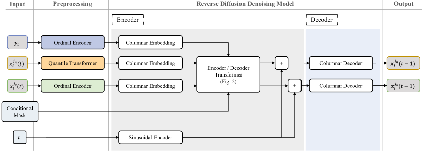
Figure 1. MTabGen flow for the classification case

4.1. Problem definition

We focus on tabular datasets for supervised tasks $D=\left\{x^{j_{c}}_{i},x^{j_{n}}_{i},y_{i}\right\}_{i=1}^{N}$ where $x^{j_{n}}_{i}$ with $j_{n}\in\left[1,K_{num}\right]$ is the set of numerical features, $x^{j_{c}}_{i}$ with $j_{c}\in\left[1,K_{cat}\right]$ is the set of categorical features, $y_{i}$ is the label, $i\in\left[1,N\right]$ counts the dataset rows, $N$ is the total number of rows and $K=K_{num}+K_{cat}$ is total number of features.

We apply a consistent preprocessing procedure across our benchmark datasets, using the Gaussian quantile transformation from the scikit-learn library [41] on numerical features and ordinal encoding for categorical ones. In our approach, we model numerical features with Gaussian diffusion and categorical features with multinomial diffusion. Each feature is subjected to a distinct forward diffusion procedure, which means that the noise components for each feature are sampled individually.

MTabGen generalizes the approach of TabDDPM where the model learns $p\left(x_{t-1}\middle|x_{t},y\right)$, i.e. the probability distribution of $x_{t-1}$ given $x_{t}$ and the target $y$. We extend this by allowing conditioning on a target variable $y$ and a subset of input features, aligning with the strategies proposed by Zheng and Charoenphakdee [65] and Tashiro et al. [49]. Specifically, we partition variable $x$ into $x^{M}$ and $\bar{x}^{M}$. Here, $x^{M}$ refers to the masked variables set, those perturbed by the forward diffusion process, while $\bar{x}^{M}$ represents the untouched variable subset that conditions the reverse diffusion. This setup models $p\left(x^{M}_{t-1}\middle|x^{M}_{t},\bar{x}^{M},y\right)$, with $\bar{x}^{M}$ remaining constant across timesteps $t$. This approach not only enhances model performance in data generation, but it also enables the possibility of performing data imputation with the same model.

The reverse diffusion process $p\left(x^{M}_{t-1}\middle|x^{M}_{t},\bar{x}^{M},y\right)$ is parameterized by the neural network shown in Figs. 1, 2 and 3. In the case of numerical features, the denoising model has to estimate the amount of noise added between steps $t-1$ and $t$ in the forward diffusion process, and in the case of categorical features, it must predict the (logit of) distribution of the categorical variable a $t=0$. The model output has therefore dimensionality of $K_{num}+\sum_{i=1}^{K_{cat}}Cl_{i}$ where $Cl_{i}$ is the number of classes of $i$-th categorical feature.

4.2. Model Overview

As shown in Figs. 1, 2 and 3, the denoising model is based on an encoder-decoder structure. The encoder obtains a representation of each feature in two steps. Initially, a columnar embedding projects individually all the heterogeneous features (continuous or categorical) in the same homogeneous and dense latent space. Then, a conditional encoder-decoder transformer embedding enhances the latent representation of features by considering their interactions with each other and with the condition. For the columnar embedding of categorical and numerical features, we utilize an embedding layer and a linear-ReLU activation layer, respectively. The type of task (regression or classification) dictates the choice of embedding for the target (y).

The conditional encoder-decoder transformer (detailed in Fig. 2) incorporates the output of columnar embedding through specialized masking. More specifically, the encoder focuses on the variables $\bar{x}^{M}$ and $y$ (i.e. conditioning variables), while the decoder attends to all the available information, $x^{M}$, $\bar{x}^{M}$ and $y$. In this setup, the encoder output provides context from conditioning variables not involved in the forward diffusion process, allowing the decoder to derive representations for those that are. Features involved in the forward diffusion process are denoted with $\texttt{Mask}=1$, and those that aren’t with $\texttt{Mask}=0$. Consequently, the encoder takes in $1-\texttt{Mask}$. When the original dataset contains missing values, a new MissingMask is introduced. More concretely, the MissingMask is combined with the conditioning Mask to remove any missing value from the condition. This mechanism allows the model to work without any type of missing data preprocessing.

We note that the encoder’s output is converted into a set of attention vectors. Specifically, the decoder integrates these vectors into its attention mechanism (Fig. 3) as the K and V vectors described in [54]. This allows the decoder to focus on the relevant features of the condition and their interactions with the masked features. This conditioning mechanism is more general and exhibits less learning bias compared to recent approaches in the literature on diffusion models for tabular data, such as TabDDPM and TabCSDI, where the condition embedding is only added to the masked feature embedding. This advantage holds true even in scenarios where the encoder processes only one variable (the target variable of a supervised task). Here, the transformer encoder functions similarly to an MLP, but its output continues to be used in the decoder’s attention mechanism, enhancing overall performance (see discussion on ablation study in Sec. 6).

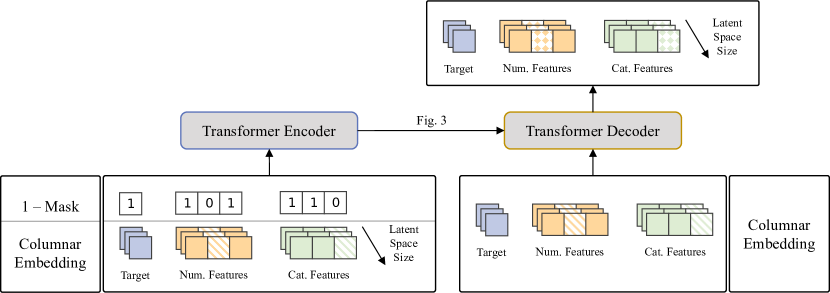
Figure 2. Conditional Transformer Encoder: In the input of the encoder-decoder transformer, the embedding of a conditioning feature is represented by a fully filled square ($\texttt{Mask}=0$), and the embedding of a masked feature is depicted by a color-dashed square ($\texttt{Mask}=1$). The encoder’s task is to learn a representation of the conditioning features, using only those marked with $\texttt{Mask}=0$. On the other hand, the decoder focus on improving the representation of the masked features ($\texttt{Mask}=1$), utilizing all available features, both conditioning and masked, along with the context generated by the encoder. The square filled with colored rhombuses in the output of the decoder correspond with the improved representation of the masked features (i.e., $\texttt{Mask}=1$). When the original dataset contains missing values, a new MissingMask is introduced. The MissingMask is combined with the conditioning Mask to remove missing value from the condition.

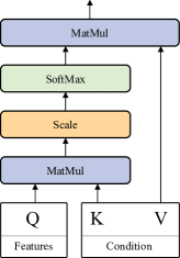
Figure 3. Conditioning Attention Mechanism: The condition embedding produced by the transformer encoder is used in the decoder attention mechanism. More in details, the condition embedding plays the roles of K and V whereas the feature embedding plays the role of Q.

The final latent feature representation is obtained by summing the conditional encoder-decoder transformer output with the timestep embedding, which is derived by projecting the sinusoidal time embedding [38, 10] into the transformer embedding dimension, using a linear layer followed by the Mish activation function [35]. Last, this representation is decoded to produce the output. Each feature has its own decoder consisting of two successive blocks integrating a linear transformation, normalization, and ReLU activation. Depending on the feature type (numerical or categorical), an additional linear layer is appended with either a singular output for numerical features or multiple outputs, corresponding to the number of classes for categorical ones.

The model is trained by minimizing a sum of mean-squared error $L^{simple}_{t}$ (Eq. 8) for the Gaussian diffusion term and the KL divergences $L^{i}_{t}$ for each multinomial diffusion term (Eq. 1).

$$L^{MTabGen}_{t}= \dfrac{L^{simple}_{t}(\texttt{Mask})}{K_{num}}+\dfrac{\sum_{i\leq K_{cat}}L^{i}_{t}(\texttt{Mask})/Cl_{i}}{K_{cat}}$$

where $L^{simple}_{t}(\texttt{Mask})$ and $L^{i}_{t}(\texttt{Mask})$ means that the loss functions are computed taking into account only the prediction error on variables affected by the forward diffusion process (i.e. $x^{M}$), $Cl_{i}$ is the number of classes of the $i$-th categorical variable.

4.3. Dynamic Conditioning

A key feature of the proposed solution is that the split between $x^{M}$ and $\bar{x}^{M}$ does not have to be fixed for all the row $i$ in the dataset. The transformer encoder can manage mask with an arbitrary number of zeros/ones, so we can dynamically alter the split between $x^{M}$ and $\bar{x}^{M}$ by just producing a new mask. In the extreme scenario, we can generate a new mask $\texttt{Mask}_{i}$ for each row $i$. During training, the number of ones in $\texttt{Mask}_{i}$ (i.e. the number of features to be included in the forward diffusion process) is uniformly sampled from the interval $[1,K_{num}+K_{cat}]$. A model that has been trained in this manner can then be used for both tasks, that is, generation of synthetic data ($\texttt{Mask}_{i}=1$ for all the $K_{num}+K_{cat}$ features and for any dataset index $i$) and imputation of missing values (for each $i$, $\texttt{Mask}_{i}=1$ for the feature to impute). As discussed, when the original dataset contains missing values, a new MissingMask is introduced and combined with the conditioning Mask to remove any missing value from the condition. The MissingMask is fixed and constant during the training phase. This setup allows for more flexible conditioning scenarios.

Specifically:

• When $\bar{x}^{M}=\emptyset$, $p\left(x^{M}_{t-1}\middle|x^{M}_{t},\bar{x}^{M},y\right)=p\left(x_{t-1}\middle|x_{t},y\right)$ our model aligns with TabDDPM, generating synthetic data influenced by the target distribution.

• When $\bar{x}^{M}\neq\emptyset$, the model can generate synthetic data based on the target distribution and either a fixed or dynamic subset of features. Conditioning on a fixed subset introduces advantages in settings where certain variables are readily accessible, whereas others are difficult to obtain due to challenges like cost constraints. In such cases, the scarce data can be synthetically produced using the known variables. Conversely, when conditioning on a dynamic subset of features, the model effectively addresses the challenge of imputing gaps within a dataset.

5. Experiments

5.1. Data

Below we introduce the benchmark datasets used in the performance evaluation of our model. The statistics are summarized in Table 1.

• HELOC [14]: Home Equity Line of Credit (HELOC) provided by FICO (a data analytics company), contains anonymized credit applications of HELOC credit lines. The dataset contains 21 numerical and two categorical features characterizing the applicant to the HELOC credit line. The task is a binary classification and the goal is to predict whether the applicant will make timely payments over a two-year period.

• Churn Modelling [21]: This dataset consists of six numerical and four categorical features about bank customers. The binary classification task involves predicting whether or not the customer closed their account.

• Gas Concentrations [55]: The dataset contains measurements from 16 chemical sensors exposed to six gases at different concentration levels. It contains $13.9$M of rows and $129$ continuous features and the classification task is to determine which is the gas generating the data.

• California Housing [40]: The information refers to the houses located in a certain California district, as well as some basic statistics about them based on 1990 census data. This is a regression task about forecasting the price of a property.

• House Sales King Country [25]: Similar to the California Housing case, this regression task involves estimating property prices in the King County region for sales between May 2014 and May 2015. The original dataset included 14 numerical features, four categorical features, and one date feature. During pre-processing, the date feature was transformed into two categorical variables: month and year.

• Adult Incoming [3]: Personal details such as age, gender or education level are used to predict whether an individual would earn more or less than 50K$\$$ per year.

• Otto Group [4]: This dataset, provided by the Otto Group (an e-commerce company), contains $61.9$K of rows and $93$ continuous product attributes. The task is a multi-class classification problem with nine categories, aiming to determine the category to which each product belongs.

• Cardiovascular Disease [51]: The existence or absence of cardiovascular disease must be predicted based on factual information, medical examination results, and information provided by the patient. The dataset consists of seven numerical and four categorical features.

• Insurance [43]: Customer variables and past payment data are used to solve a binary task: determining whether the customer will pay on time. The dataset has eight numerical and two categorical features.

• Forest Cover Type [7]: In this multi-class classification task with seven categories, cartographic variables are used to predict the forest cover type. The first eight features of the dataset are continuous, whereas the last two are categorical with four and 40 levels respectively.

Table 1. Tabular benchmark properties.

Dataset	Rows	Num. Feats	Cat. Feats	Task
HELOC	9871	21	2	Binary
Churn	10000	6	4	Binary
Gas Concentrations	13910	129	0	Multi-Class ($6$)
Cal. Hous.	20640	8	0	Regression
House Sales	21613	14	2	Regression
Adult Inc.	32561	6	8	Binary
Otto Group	61900	93	0	Multi-Class ($9$)
Cardio	70000	7	4	Binary
Insurance	79900	8	2	Binary
Forest Cov.	581 K	10	2	Multi-Class (7)

5.2. Baselines

For the synthetic data generation task, we consider the following state-of-the-art baselines drawn from representative generative modeling paradigms: VAE, GAN and Diffusion Models:

• TabDDPM [30]: State-of-the-art diffusion model for tabular data generation and model in which we have premised the proposed approach.

• Tabsyn [62]: Recent state-of-the-art tabular generative model that integrates a diffusion model into the continuous latent space projected by a VAE.

• CoDi [32]: A diffusion model for tabular data generation. The StaSy and CoDi models are from the same team. In [32], the authors show that CoDi consistently outperforms StaSY. Therefore, we only include CoDi in our evaluation.

• TVAE [59]: A variational autoencoder adapted for mixed-type tabular data.

• CTGAN5 [59]: A conditional GAN for synthetic tabular data generator.

For the missing data imputation task, the following state-of-the-art baselines have been considered:

• missForest [48]: Iterative method based on random forests to predict and fill in missing values.

• GAIN6 [60]: GAN model for tabular missing value imputation.

• HyperImpute6 [23]: Iterative imputation algorithm using both regression and classification methods based on linear models, trees, XGBoost, CatBoost and neural nets.

• Miracle6 [31]: Missing imputation algorithm using a causal deep learning approach.

• TabCSDI [65]: State-of-the-art diffusion model for missing data imputation.

5.3. Metrics

We evaluate the generative models on three different dimensions: (1) ML efficiency, (2) statistical similarity and (3) privacy risk.

5.3.1. Machine Learning efficiency

The Machine Learning efficiency measures the performance degradation of classification or regression models trained on synthetic data, and then tested on real data. The basic idea is to use a ML discriminative model to evaluate the utility of synthetic data provided by a generative model. As demonstrated by Kotelnikov et al. [30], a strong ML model allows to obtain more stable and consistent conclusions on the performances of the generative model. Based on this intuition, we consider 4 different ML models: XGBoost [8], CatBoost [42], LightGBM [27] and MLP. We introduce an initial fine-tuning step, during which we derive the best hyperparameter configuration using the Optuna library [2]. Specifically, we perform 100 iterations to fine-tune the model’s (XGBoost, CatBoost, LightGBM and MLP) hyperparameters on each dataset’s real data within the benchmark. Every hyperparameter configuration for ML model is cross-validated, using a five-fold split. The complete hyperparameter search space is shown in appendix A Table 7.

Once the discriminative model has been optimized for each dataset, the generative model is further cross-validated using a five-fold split, by implementing the following procedure. For each fold, the real data is split into three subsets. The main purpose of the first subset is to train the generative model. The resulting model generates a synthetic dataset conditioned on the second subset. The synthetic dataset is then used to train the discriminative model. The so-obtained ML model is finally tested on the third held-out subset, which has not been used in training any of the models. The procedure is repeated for each fold, and the obtained metric mean is used as a final measure to compute the generative model ML efficiency.

5.3.2. Statistical similarity

The comparison between synthetic and real data accounts for both individual and joint feature distributions. Adopting the approach proposed by Zhao et al. [64], we employ Wasserstein [56] and Jensen-Shannon distances [33] to analyze numerical and categorical distributions. In addition, we use the square difference between pair-wise correlation matrix to evaluate the preservation of feature interactions in synthetic datasets. Specifically, the Pearson correlation coefficient measures correlations between numerical features, the Theil uncertainty coefficient measures correlations between categorical features, and the correlation ratio evaluates interactions between numerical and categorical features.

5.3.3. Privacy Risk

The Privacy Risk is evaluated using the Distance to Closest Record (DCR), i.e. the Euclidean distance between any synthetic record and its closest corresponding real neighbour. Ideally, the higher the DCR the lesser the risk of privacy breach. It is important to note that out-of-distribution data, i.e. random noise, will also produce high DCR. Therefore, to maintain ecological validity, the DCR metric needs to be evaluated jointly with the ML efficiency metric.

6. Results

6.1. Machine Learning efficiency

6.1.1. Synthetic data generation

In this task, we evaluate the performance of our generative model in producing high-quality synthetic data, conditioned exclusively by the supervised target $y$. To this end, we consider two variants of our model:

1. MTabGen I: This variant consistently includes all dataset features in the diffusion process and was specifically designed for the synthetic data generation task.

2. MTabGen II: During training, this variant dynamically selects which features are incorporated in the diffusion process, making it versatile for both imputing missing data and generating complete synthetic datasets.

Table 2. Machine Learning efficiency. Classification tasks use F1-score, and regression tasks use MSE, indicated by up/down arrows for maximization/minimization of the metric. Cross-validation mean and standard deviation are shown for each dataset-model pair. Best and second-best results are highlighted in bold and underline, respectively. Baseline column shows average performance of ML models trained on real data, while other columns reflect average performance of ML models trained on synthetic data from specified models. All models are tested on real data.

Dataset	Baseline	TVAE	CTGAN	CoDi	Tabsyn	TabDDPM	MTabGen I	MTabGen II
HELOC $\uparrow$	$83.69\pm 0.04$	$79.41\pm 0.05$	$77.53\pm 0.06$	$75.82\pm 0.07$	$79.24\pm 0.05$	$76.69\pm 0.10$	$\mathbf{82.91\pm 0.07}$	$\underline{82.71\pm 0.08}$
Churn $\uparrow$	$85.25\pm 0.05$	$81.67\pm 0.08$	$79.31\pm 0.06$	$82.77\pm 0.15$	$\mathbf{84.60\pm 0.06}$	$83.62\pm 0.15$	$\underline{84.43\pm 0.03}$	$83.91\pm 0.04$
Gas $\uparrow$	$99.47\pm 0.09$	$94.55\pm 0.07$	$62.04\pm 0.07$	$65.41\pm 0.04$	$\underline{98.66\pm 0.04}$	$65.51\pm 0.06$	$\mathbf{98.80\pm 0.07}$	$98.60\pm 0.06$
Cal. Hous. $\downarrow$	$0.161\pm 0.001$	$0.316\pm 0.003$	$0.488\pm 0.004$	$0.290\pm 0.003$	$0.256\pm 0.002$	$0.272\pm 0.002$	$\mathbf{0.224\pm 0.001}$	$\underline{0.227\pm 0.001}$
House Sales $\downarrow$	$0.101\pm 0.001$	$0.209\pm 0.001$	$0.335\pm 0.001$	$0.159\pm 0.001$	$0.148\pm 0.001$	$\underline{0.145\pm 0.001}$	$\mathbf{0.121\pm 0.001}$	$\underline{0.145\pm 0.001}$
Adult Inc. $\uparrow$	$86.95\pm 0.04$	$84.34\pm 0.07$	$83.64\pm 0.08$	$84.43\pm 0.08$	$84.70\pm 0.06$	$84.86\pm 0.07$	$\mathbf{85.30\pm 0.09}$	$\underline{85.15\pm 0.07}$
Otto $\uparrow$	$81.50\pm 0.06$	$63.87\pm 0.05$	$50.48\pm 0.05$	$63.21\pm 0.06$	$67.14\pm 0.08$	$63.34\pm 0.08$	$\mathbf{73.04\pm 0.07}$	$\underline{72.98\pm 0.06}$
Cardio $\uparrow$	$73.54\pm 0.05$	$72.47\pm 0.08$	$71.81\pm 0.06$	$72.34\pm 0.10$	$\underline{72.90\pm 0.11}$	$72.88\pm 0.14$	$\mathbf{72.97\pm 0.08}$	$72.67\pm 0.12$
Insurance $\uparrow$	$92.00\pm 0.03$	$92.63\pm 0.11$	$92.56\pm 0.05$	$92.03\pm 0.07$	$92.20\pm 0.05$	$92.21\pm 0.04$	$\mathbf{92.77\pm 0.11}$	$\underline{92.64\pm 0.07}$
Forest Cov. $\uparrow$	$96.42\pm 0.06$	$70.36\pm 0.04$	$65.65\pm 0.07$	$74.64\pm 0.09$	$74.83\pm 0.10$	$82.08\pm 0.07$	$\mathbf{85.61\pm 0.04}$	$\underline{84.32\pm 0.09}$
Average Rank		$4.9$	$6.5$	$5.7$	$3.3$	$4.0$	$\mathbf{1.1}$	$\underline{2.4}$

The results shown in Table 2 indicate that MTabGen II outperforms existing state-of-the-art methods like TabDDPM, Tabsyn, CoDi, TVAE, or CTGAN in the synthetic data generation task, with the exception of the specialized MTabGen I which achieves better performance. The key outcomes of our experiments are as follows: (1) TVAEproduces better results than CTGAN. (2) Approaches based on Diffusion Models outperform TVAE and CTGAN in mean. (3) Our two proposed models systematically enhance the performance of TabDDPM, Tabsyn and CoDi, obtaining the best results across all datasets included in our benchmark. (4) Our model tends to outperform the baselines in datasets with a large number of features, such as the Gas Concentrations and Otto Group datasets, although this trend is less consistent with Tabsyn. Additionally, it is worth noting that the ML efficiency results align with those reported in the Tabsyn paper, where Tabsyn generally surpasses TabDDPM and CoDi, with TVAE also showing stronger performance than CoDi.

The results presented in Table 2 are obtained after applying an optimisation step for each generative model, using the Optuna library over $100$ trials, and evaluating performance with the cross-validated ML efficiency metric defined in Section 5.3 as the objective. The specific hyperparameters search space for each model is shown in Table 8, appendix A.

6.1.2. Ablation study

We conduct an ablation study to evaluate the contributions of the encoder-decoder transformer and dynamic conditioning to our model’s performance and usability. The encoder-decoder transformer enhances performance for two primary reasons:

• Enhanced learning of inter-feature interactions within condition (encoder) and masked features (decoder). Transformer layers allow for better learning of inter-feature interactions compared to MLPs. This is primarily due to the attention mechanism, where the new embedding of a feature $x_{i}$ is computed by a linear combination of the embeddings of all features $\{x_{j}\}$. The weight of feature $x_{j}$ depends on the current values of $x_{i}$ and $x_{j}$. This mechanism is more flexible than in MLP case, where the contribution of feature $x_{j}$ to a neuron in the next layer is fixed and does not depend on its current value.

• Conditioning attention mechanism. Our model, MTabGen, uses an encoder-decoder transformer architecture. The encoder learns latent representations of unmasked features for conditioning, while the decoder focuses on learning latent representations of masked or noisy features. By incorporating conditioning within the attention mechanism of the transformer decoder, we reduce learning bias compared to conventional methods like those used in TabDDPM, which simply sum the latent representations of conditions and noisy features.

To test the impact of these hypotheses, we modified the original implementation of TabDDPM by replacing the MLP denoising model with a transformer encoder, while retaining the same conditioning mechanism (i.e., summing the condition embedding and feature embedding). We call this new implementation TabDDPM-Transf. As shown in the first two columns of Table 3, our transformer-enhanced TabDDPM-Transf consistently outperforms the standard TabDDPM. The impact of the conditioning attention mechanism is further demonstrated by the comparison of TabDDPM-Transf and MTabGen I in Table 3.

Table 3. Ablation study in terms of Machine Learning efficiency. Classification tasks use F1-score, and regression tasks use MSE, indicated by up/down arrows for maximization/minimization of the metric. Cross-validation mean and standard deviation are shown for each dataset-model pair. Best and second-best results are highlighted in bold and underline, respectively. Baseline column shows average performance of ML models trained on real data, while other columns reflect average performance of ML models trained on synthetic data from specified models. All models are tested on real data.

Dataset	Baseline	TabDDPM	TabDDPM-Transf	MTabGen I
HELOC $\uparrow$	$83.69\pm 0.04$	$76.69\pm 0.10$	$\underline{81.15\pm 0.08}$	$\mathbf{82.91\pm 0.07}$
Churn $\uparrow$	$85.25\pm 0.05$	$83.62\pm 0.15$	$\underline{83.62\pm 0.05}$	$\mathbf{84.43\pm 0.03}$
Gas $\uparrow$	$99.47\pm 0.09$	$65.51\pm 0.06$	$\underline{93.35\pm 0.09}$	$\mathbf{98.80\pm 0.09}$
Cal. Hous. $\downarrow$	$0.161\pm 0.001$	$0.272\pm 0.001$	$\underline{0.232\pm 0.001}$	$\mathbf{0.224\pm 0.001}$
House Sales $\downarrow$	$0.101\pm 0.001$	$0.145\pm 0.001$	$\underline{0.128\pm 0.001}$	$\mathbf{0.121\pm 0.001}$
Adult Inc. $\uparrow$	$86.95\pm 0.04$	$84.86\pm 0.07$	$\underline{85.13\pm 0.06}$	$\mathbf{85.30\pm 0.09}$
Otto $\uparrow$	$81.50\pm 0.06$	$63.34\pm 0.08$	$\underline{71.01\pm 0.08}$	$\mathbf{73.04\pm 0.07}$
Cardio $\uparrow$	$73.54\pm 0.05$	$72.88\pm 0.14$	$\underline{72.94\pm 0.11}$	$\mathbf{72.97\pm 0.08}$
Insurance $\uparrow$	$92.00\pm 0.03$	$92.21\pm 0.04$	$\underline{92.69\pm 0.06}$	$\mathbf{92.77\pm 0.11}$
Forest Cov. $\uparrow$	$96.42\pm 0.06$	$82.08\pm 0.07$	$\underline{83.84\pm 0.08}$	$\mathbf{85.61\pm 0.04}$

With respect to model usability, dynamic conditioning allows a single model to handle a variety of tasks without compromising performance. Notably, performance metrics for our multi-tasking model, MTabGen II (with dynamic conditioning), align closely with those of our specific data generation model, MTabGen I (without dynamic conditioning), as shown in Table 2. Dynamic conditioning supports not only synthetic data generation and missing data imputation but also “prompted data generation” - a scenario where a synthetic subset of features is generated based on a known subset of variables. This method is particularly useful in settings where data collection is challenging, enhancing data augmentation in ML projects, improving customer profiling, or acting as a simulated environment in reinforcement learning, which accelerates data-generation efforts.

6.1.3. Missing data imputation

Here, we report the results of our experiments on evaluating the models’ ability to impute missing values. Specifically, in this task, the generative model utilizes the available data to condition the generation of data for the missing entries.

Following the example of [60] and [65], the evaluation of imputed data quality is carried out in the Missing Completely at Random (MCAR) setup, under the assumption that the probability for missing data is uniformly distributed across observations and columns. To this end, we initially divide the dataset into two subsets: $70\%$ “imputation training” set and $30\%$ hold-out. Then, we construct three different versions of the $70\%$ “imputation training” split, each with increasing percentage of missing data: $10\%$, $25\%$, and $40\%$, while keeping the hold-out split intact. To evaluate the quality of imputed data in terms of ML efficiency, we apply the steps described in Alg. 1.

Algorithm 1 Evaluate Imputation Model Performance

1:for each dataset in the benchmark do

2:     for each percentage of missing values in $\left\{10\%,25\%,40\%\right\}$ do

3:         Employ the generative model to fill in the missing values in the $70\%$ training subset.

4:         Train the ML discriminative model (e.g., XGBoost, CatBoost, LightGBM and MLP) on the imputed data.

5:         Evaluate the ML discriminative model on the hold-out $30\%$ subset.

6:     end for

7:end for

Our findings, detailed in Table 4, show that MTabGen consistently outperforms the baseline models considered in this step: missForest [48], GAIN [60], HyperImpute [23], Miracle [31], and TabCSDI [65]. Across all levels of missing data, MTabGen outperforms on average the baselines, and introduces a performance advantage that increases proportionally to the volume of missing data.

Table 4. Missing imputation analysis in terms of Machine Learning efficiency. Classification tasks use F1-score, and regression tasks use MSE, indicated by up/down arrows for maximization/minimization of the metric. Cross-validation mean and standard deviation are shown for each dataset-model pair. Best and second-best results are highlighted in bold and underline, respectively.

Dataset	$\%$ Missing	missForest	GAIN	HyperImpute	Miracle	TabCSDI	MTabGen
	$10\%$	$83.16\pm 0.02$	$82.44\pm 0.02$	$83.36\pm 0.04$	$\underline{83.39\pm 0.03}$	$83.30\pm 0.05$	$\mathbf{83.79\pm 0.03}$
HELOC $\uparrow$	$25\%$	$82.80\pm 0.04$	$81.92\pm 0.04$	$83.23\pm 0.04$	$82.85\pm 0.04$	$\underline{83.27\pm 0.04}$	$\mathbf{83.54\pm 0.04}$
	$40\%$	$82.59\pm 0.04$	$81.74\pm 0.03$	$\underline{82.97\pm 0.03}$	$82.74\pm 0.03$	$82.67\pm 0.03$	$\mathbf{83.41\pm 0.04}$
	$10\%$	$84.49\pm 0.03$	$\underline{84.66\pm 0.03}$	$84.47\pm 0.05$	$84.60\pm 0.03$	$84.48\pm 0.03$	$\mathbf{84.76\pm 0.03}$
Churn $\uparrow$	$25\%$	$\underline{84.13\pm 0.03}$	$83.45\pm 0.05$	$83.89\pm 0.05$	$84.08\pm 0.03$	$83.92\pm 0.03$	$\mathbf{84.51\pm 0.04}$
	$40\%$	$83.08\pm 0.04$	$83.22\pm 0.04$	$83.14\pm 0.04$	$82.52\pm 0.04$	$\underline{83.45\pm 0.04}$	$\mathbf{84.18\pm 0.04}$
	$10\%$	$0.182\pm 0.002$	$0.182\pm 0.002$	$\underline{0.173\pm 0.002}$	$0.174\pm 0.002$	$0.175\pm 0.002$	$\mathbf{0.170\pm 0.002}$
Cal. Hous. $\downarrow$	$25\%$	$0.229\pm 0.002$	$0.249\pm 0.002$	$0.190\pm 0.002$	$0.196\pm 0.002$	$\underline{0.188\pm 0.003}$	$\mathbf{0.183\pm 0.002}$
	$40\%$	$0.269\pm 0.004$	$0.306\pm 0.004$	$\underline{0.218\pm 0.003}$	$0.269\pm 0.004$	$0.258\pm 0.004$	$\mathbf{0.210\pm 0.003}$
	$10\%$	$0.109\pm 0.002$	$0.110\pm 0.002$	$0.112\pm 0.002$	$\underline{0.106\pm 0.002}$	$0.110\pm 0.002$	$\mathbf{0.105\pm 0.002}$
House Sales $\downarrow$	$25\%$	$0.118\pm 0.002$	$0.131\pm 0.003$	$0.120\pm 0.003$	$0.127\pm 0.002$	$\underline{0.117\pm 0.003}$	$\mathbf{0.115\pm 0.002}$
	$40\%$	$0.155\pm 0.003$	$0.145\pm 0.003$	$0.156\pm 0.003$	$0.130\pm 0.003$	$\underline{0.128\pm 0.003}$	$\mathbf{0.119\pm 0.002}$

6.2. Statistical Similarity

In this task, we compare synthetic and real data accounts based on individual and joint feature distributions. We report only the top three models with the best ML efficiency. This approach is motivated by our findings, which show a strong association between the ML efficiency of synthetic data and their ability to replicate the statistical properties of real data. In other words, synthetic data with higher ML utility tends to better reproduce both individual and joint feature distributions.

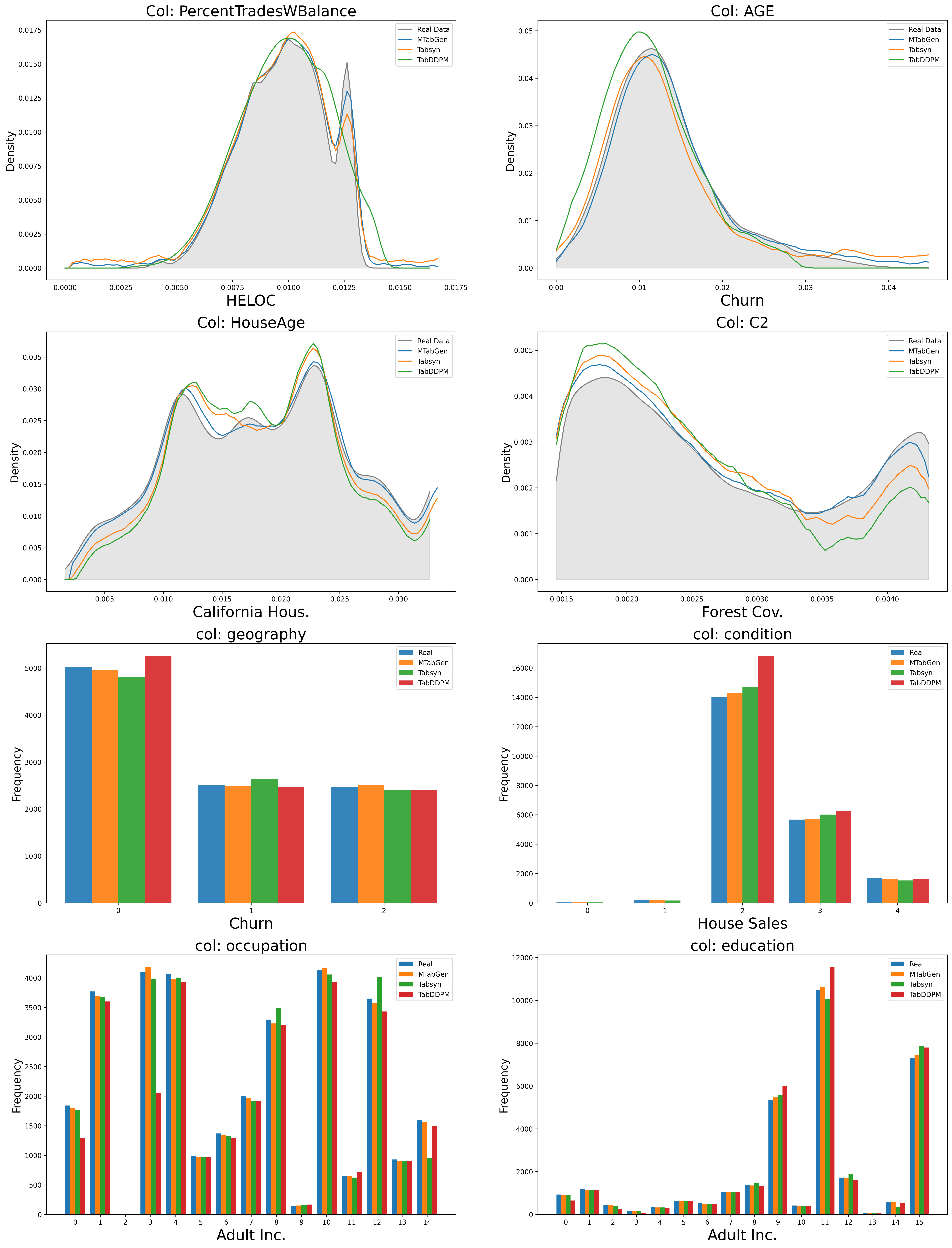
Figure 4. Comparison between distribution of real and synthetic data. The two top rows present four examples of numerical columns from various datasets in our benchmark, while the two bottom rows contain examples of categorical features.

Table 5. Statistical similarity details

(a) Average Wasserstein Distance	(b) Average Jensen-Shannon Distance	(c) Average L2 Dist. Correlation Matrix
Dataset Tabsyn TabDDPM MTabGen HELOC $\underline{0.25\pm 0.03}$ $0.29\pm 0.02$ $\mathbf{0,15\pm 0.02}$ Churn $\mathbf{0.15\pm 0.02}$ $0.23\pm 0.02$ $\underline{0.17\pm 0.02}$ Gas $\mathbf{0.21\pm 0.04}$ $0.65\pm 0.06$ $\underline{0.23\pm 0.02}$ Cal.Hous $\underline{0.31\pm 0.03}$ $0.34\pm 0.04$ $\mathbf{0.22\pm 0.02}$ House Sales $0.32\pm 0.02$ $\underline{0.28\pm 0.03}$ $\mathbf{0.15\pm 0.01}$ Adult Inc. $\mathbf{0.18\pm 0.03}$ $0.24\pm 0.02$ $\underline{0.19\pm 0.02}$ Otto $\underline{0.25\pm 0.02}$ $0.27\pm 0.03$ $\mathbf{0.16\pm 0.02}$ Cardio $\mathbf{0.23\pm 0.04}$ $0.26\pm 0.03$ $\underline{0.24\pm 0.03}$ Insurance $\mathbf{0.19\pm 0.02}$ $0.22\pm 0.02$ $\underline{0.20\pm 0.03}$ Forest Cov. $0.41\pm 0.05$ $\underline{0.35\pm 0.04}$ $\mathbf{0.18\pm 0.02}$ Av. Rank $\underline{1.7}$ $2.8$ $\mathbf{1.5}$	Dataset Tabsyn TabDDPM MTabGen HELOC $\underline{0.15\pm 0.02}$ $0.20\pm 0.02$ $\mathbf{0,08\pm 0.01}$ Churn $\mathbf{0.07\pm 0.01}$ $0.15\pm 0.02$ $\underline{0.09\pm 0.01}$ Gas NA NA NA Cal.Hous NA NA NA House Sales $\underline{0.22\pm 0.02}$ $0.26\pm 0.03$ $\mathbf{0.09\pm 0.01}$ Adult Inc. $\mathbf{0.07\pm 0.01}$ $0.14\pm 0.02$ $\underline{0.08\pm 0.02}$ Otto NA NA NA Cardio $\mathbf{0.10\pm 0.01}$ $0.14\pm 0.02$ $\underline{0.11\pm 0.01}$ Insurance $\mathbf{0.09\pm 0.01}$ $0.13\pm 0.01$ $\underline{0.10\pm 0.01}$ Forest Cov. $0.24\pm 0.03$ $\underline{0.16\pm 0.02}$ $\mathbf{0.08\pm 0.01}$ Av. Rank $\mathbf{1.6}$ $2.9$ $\mathbf{1.6}$	Dataset Tabsyn TabDDPM MTabGen HELOC $\underline{0.036\pm 0.004}$ $0.040\pm 0.004$ $\mathbf{0,025\pm 0.003}$ Churn $\mathbf{0.027\pm 0.003}$ $0.034\pm 0.003$ $\underline{0.028\pm 0.003}$ Gas $\mathbf{0.032\pm 0.003}$ $0.078\pm 0.007$ $\underline{0.034\pm 0.004}$ Cal.Hous $\underline{0.042\pm 0.004}$ $0.045\pm 0.005$ $\mathbf{0.031\pm 0.003}$ House Sales $0.044\pm 0.004$ $\underline{0.039\pm 0.004}$ $\mathbf{0.024\pm 0.003}$ Adult Inc. $\mathbf{0.029\pm 0.003}$ $0.036\pm 0.004$ $\underline{0.030\pm 0.003}$ Otto $\underline{0.037\pm 0.004}$ $0.041\pm 0.004$ $\mathbf{0.026\pm 0.003}$ Cardio $\mathbf{0.032\pm 0.003}$ $0.035\pm 0.003$ $\underline{0.033\pm 0.003}$ Insurance $\underline{0.031\pm 0.003}$ $0.033\pm 0.003$ $\mathbf{0.029\pm 0.003}$ Forest Cov. $0.052\pm 0.004$ $\underline{0.046\pm 0.004}$ $\mathbf{0.031\pm 0.003}$ Av. Rank $\underline{1.8}$ $2.8$ $\mathbf{1.4}$

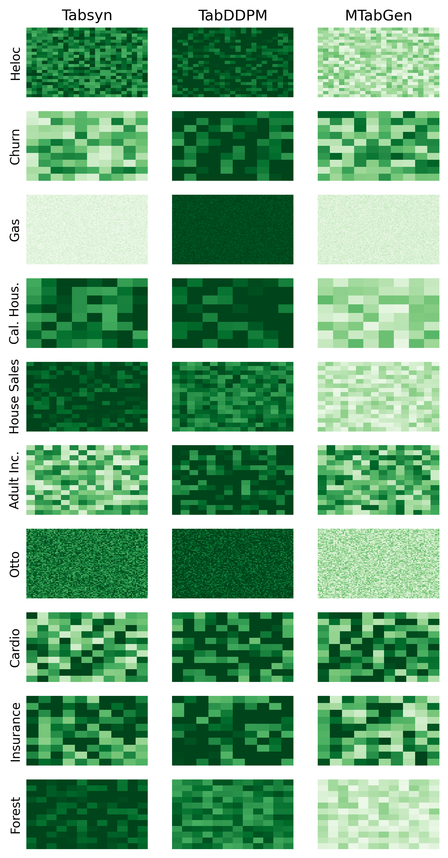
Figure 5. L2 distance between correlation matrices computed on real and synthetic data. More intense green color means higher difference between the real and synthetic correlation values.

Table 5-a shows the average Wasserstein Distance between synthetic and real numerical data distributions. Specifically, the Wasserstein distance is calculated for each numerical column between the real data and the synthetic data generated by Tabsys, TabDDPM, and MTabGen. For each generative model, the final dataset results are the average of these distances across all numerical columns in the dataset. MTabGen consistently performs better than Tabsys and TabDDPM. This advantage is more pronounced in datasets where there is a larger difference in ML efficiency, such as HELOC, California Housing, House Sales or Forest Cover Type dataset. In contrast, in datasets like Insurance, where all models have similar ML efficiency, the Wasserstein distances are also comparable. A qualitative analysis of the results for some of the columns can be found in the four plots in the two top rows of Fig. 4. These plots compare the distributions of real data with those of the synthetic data generated by the different models.

Similarly, Table 5-b shows the average Jensen-Shannon distance between synthetic and real categorical data distributions. MTabGen and Tabsyn outperform TabDDPM, consistent with the findings of [62], where Tabsyn achieved better results than TabDDPM on categorical data. Also the Jensen-Shannon distance appears to be strongly related to ML efficiency. For example, in datasets like HELOC, House Sales or Forest Cover Type, where ML efficiency of MTabGen is significantly better than the other baselines, it also has a lower Jensen-Shannon distance. In the Insurance dataset, where all baselines have similar ML efficiency, the Jensen-Shannon distances are also similar. Notably, while MTabGen and Tabsyn show similar overall results, a qualitative analysis of per-column results reveals that MTabGen tends to excel when the number of classes in the categorical variable increases, as shown in the bottom row plots of Fig. 4.

Table 5-c shows the average L2 distance between the two correlation matrices computed on real and synthetic data. Fig. 5, instead, shows the L2 distance details across all the datasets in the benchmark. In Fig. 5 more intense green color means higher difference between the real and synthetic correlation values. Even more than in the previous statistical measures, there exist an association between ML efficiency and L2 distance between correlation matrices. In datasets like HELOC, California Housing, House Sales or Forest Cover Type where the ML efficiency of MTabGen is notably better than the one of Tabsyn and TabDDPM the corresponding heatmap of MTabGen are more lighter, e.g. they shown a smaller error in the correlation estimation. Nevertheless in datasets like Cardio or Insurance where all the models perform similarly, the heatmaps do not shown resignable differences.

6.3. Privacy risk

In this section, we delve deeper into the privacy risk associated with synthetic data. As previously mentioned, DCR is defined by the Euclidean distance between any synthetic record and its closest real neighbor. Ideally, a higher DCR indicates a lower privacy risk. However, out-of-distribution data (random noise) can also result in high DCR. Therefore, to maintain ecological validity, DCR should be evaluated alongside the ML efficiency metric. For this reason, our privacy risk evaluation includes only Tabsyn, TabDDPM, and MTabGen. These models have superior ML efficiency and are more likely to pose a privacy risk (lower DCR) because they closely mimic the original data

Table 6 presents our evaluation results regarding the privacy risk metric, emphasizing the trade-off between ML efficiency and privacy guarantees. Based on a 5% threshold for relative improvement in ML efficiency of MTabGen over Tabsyn and TabDDPM, the results are categorized to illustrate two key points: (1) Improvements in ML efficiency correlate with increased privacy risks. (2) When MTabGen’s performance improvement over the baselines is less than 5%, no significant increase in privacy risk is observed. However, when MTabGen’s performance is substantially better, the comparison becomes irrelevant because the synthetic data generated by the baselines deviate significantly from real data in terms of ML utility and statistical properties, resulting in a high DCR due to poor alignment with real data properties.

Figures 6 and 7 provide a qualitative comparison of the DCR distribution for MTabGen versus Tabsyn and TabDDPM when the relative improvement in ML efficiency is less than 5%. This comparison confirms that there are no significant changes or patterns, indicating that the improvement in ML efficiency does not lead to a noticeable increase in privacy risk.

Table 6. Comparison of privacy risk ($\uparrow$) and ML efficiency ($\uparrow$ for F1-score, $\downarrow$ for MSE) for Tabsyn, TabDDPM, and MTabGen for each dataset. Privacy risk is evaluated using the Distance to Closest Record; higher values indicate a lesser risk of privacy breach. The results are divided based on a 5% ML efficiency threshold relative to the performance improvements of MTabGen compared to Tabsyn and TabDDPM. In cases where MTabGen achieves comparable ML efficiency to the baselines, the privacy risk is similar. However, in scenarios where MTabGen outperforms the other baselines, there is higher privacy risk (i.e lower value of DCR distance), as expected, since better ML efficiency is related with closer statistical fidelity of the generated data.

Tabsyn and MTabGen

Dataset	Tabsyn		MTabGen
	Risk $\uparrow$	ML eff.	Risk $\uparrow$	ML eff.
HELOC	$\mathbf{0.35}$	$79.24$ $\uparrow$	$0.25$	$\mathbf{82.91}$ $\uparrow$
Churn	$0.06$	$\mathbf{84.60}$ $\uparrow$	$\mathbf{0.09}$	$84.43$ $\uparrow$
Gas	$\mathbf{0.21}$	$98.66$ $\uparrow$	$0.19$	$\mathbf{98.80}$ $\uparrow$
Adult Inc.	$\mathbf{0.13}$	$84.70$ $\uparrow$	$0.11$	$\mathbf{85.30}$ $\uparrow$
Cardio	$0.35$	$72.90$ $\uparrow$	$\mathbf{0.41}$	$\mathbf{72.97}$ $\uparrow$
Insurance	$\mathbf{0.12}$	$92.20$ $\uparrow$	$\mathbf{0.12}$	$\mathbf{92.77}$ $\uparrow$
5% Relative ML eff. Threshold
Cal. Hous.	$\mathbf{0.81}$	$0.256$ $\downarrow$	$0.18$	$\mathbf{0.224}$ $\downarrow$
House Sales	$\mathbf{0.16}$	$0.148$ $\downarrow$	$0.10$	$\mathbf{0.121}$ $\downarrow$
Otto	$\mathbf{1.08}$	$67.14$ $\uparrow$	$0.12$	$\mathbf{73.04}$ $\uparrow$
Forest Cov.	$\mathbf{0.85}$	$74.83$ $\uparrow$	$0.35$	$\mathbf{85.61}$ $\uparrow$

TabDDPM and MTabGen

Dataset	TabDDPM		MTabGen
	Risk $\uparrow$	ML eff.	Risk $\uparrow$	ML eff.
Churn	$\mathbf{0.09}$	$83.62$ $\uparrow$	$\mathbf{0.09}$	$\mathbf{84.43}$ $\uparrow$
Adult Inc.	$\mathbf{0.15}$	$84.86$ $\uparrow$	$0.11$	$\mathbf{85.30}$ $\uparrow$
Cardio	$\mathbf{0.41}$	$72.88$ $\uparrow$	$\mathbf{0.41}$	$\mathbf{72.97}$ $\uparrow$
Insurance	$\mathbf{0.12}$	$92.21$ $\uparrow$	$\mathbf{0.12}$	$\mathbf{92.77}$ $\uparrow$
Forest Cov.	$\mathbf{0.47}$	$82.08$ $\uparrow$	$0.35$	$\mathbf{85.61}$ $\uparrow$
5% Relative ML eff. Threshold
HELOC	$\mathbf{2.75}$	$76.69$ $\uparrow$	$0.25$	$\mathbf{82.91}$ $\uparrow$
Gas	$\mathbf{3.15}$	$65.51$ $\uparrow$	$0.19$	$\mathbf{98.80}$ $\uparrow$
Cal. Hous.	$\mathbf{1.28}$	$0.272$ $\downarrow$	$0.18$	$\mathbf{0.224}$ $\downarrow$
House Sales	$\mathbf{0.34}$	$0.145$ $\downarrow$	$0.10$	$\mathbf{0.121}$ $\downarrow$
Otto	$\mathbf{2.57}$	$63.34$ $\uparrow$	$0.12$	$\mathbf{73.04}$ $\uparrow$

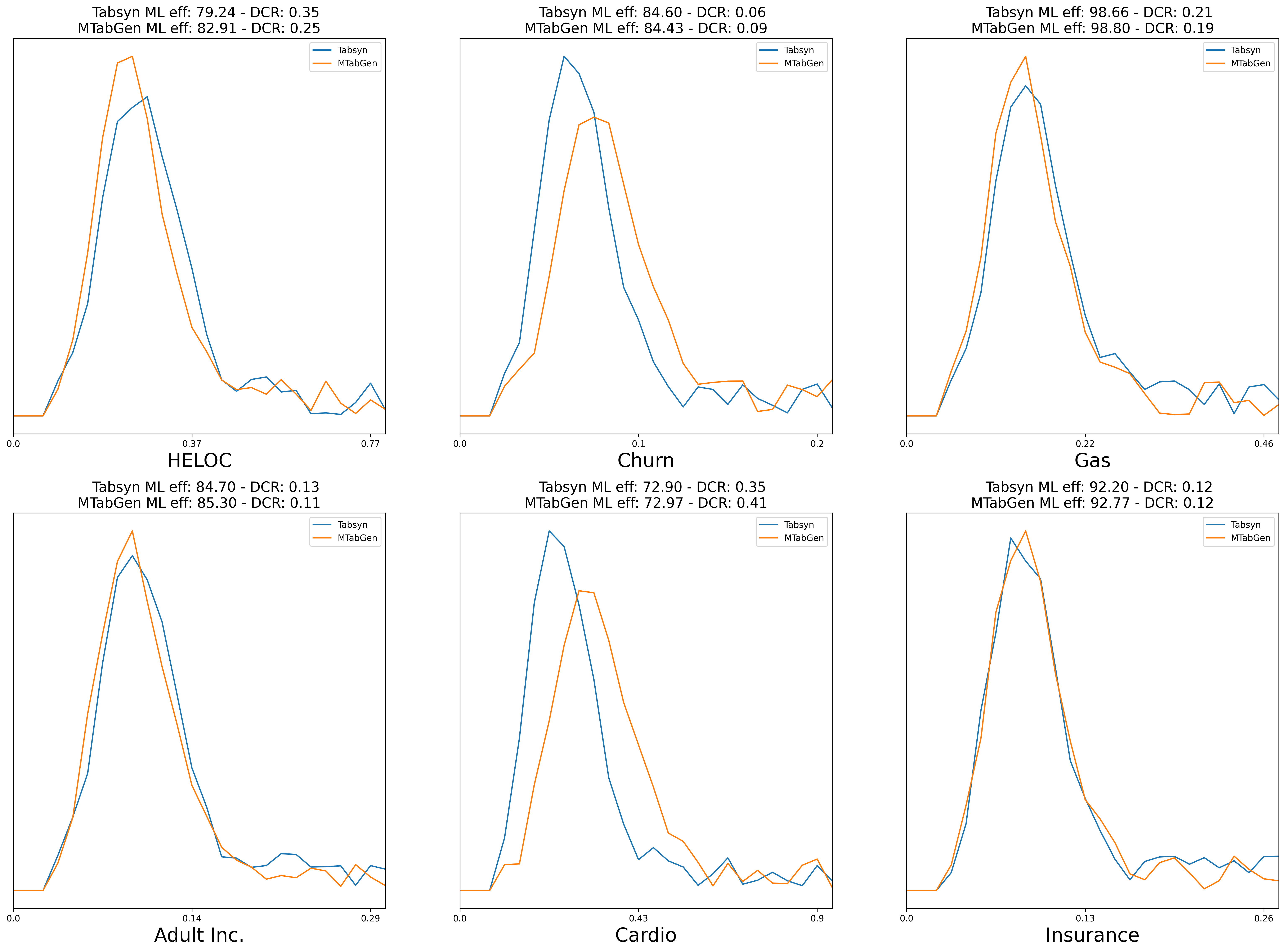
Figure 6. Distance to Closest Record (DCR) for Tabsyn and MTabGen

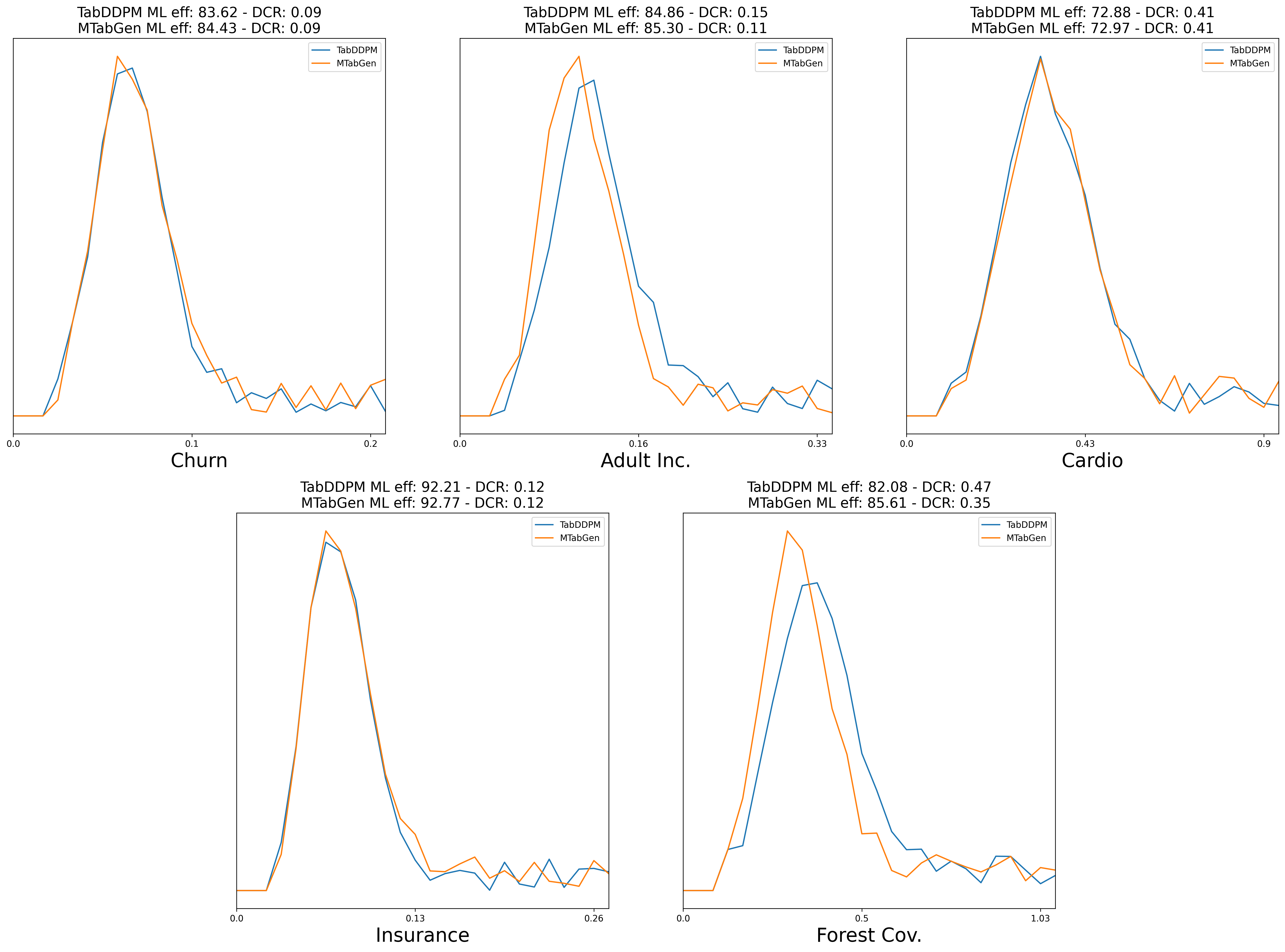
Figure 7. Distance to Closest Record (DCR) for TabDDPM and MTabGen

To mitigate the risk of increasing privacy concerns, our framework is equipped to integrate additional privacy-preserving measures, such as differential privacy [22], allowing for a better-controlled balance between data efficiency and privacy. Additionally, we conduct a sanity check to ensure that no synthetic sample perfectly matches any original sample (i.e., DCR is always greater than 0), safeguarding against direct data leakage.

7. Conclusion

In this paper, we introduced MTabGen, a diffusion model enhanced with a conditioning attention mechanism, a transformer-based encoder-decoder architecture, and dynamic masking. MTabGen is specifically designed for applications involving mixed-type tabular data. The transformer encoder-decoder acts as the denoising network, enabling the conditioning attention mechanism while effectively capturing and representing complex interactions and dependencies within the data. The dynamic masking feature allows MTabGen to handle both synthetic data generation and missing data imputation tasks within a unified framework efficiently. We proposed to train the diffusion model to regenerate masked data, enabling applications ranging from data imputation to unconditioned or conditioned synthetic data generation. This versatility makes MTabGen suitable for generating synthetic data to overcome privacy regulations, augment existing datasets, or mitigate class imbalances. We evaluated MTabGen against established baselines across several public datasets with a diverse range of features. Our model demonstrated better performance in terms of ML efficiency and statistical accuracy, while maintaining privacy risks comparable to those of the baselines, particularly showing increased performance in datasets with a large number of features.

Impact Statements

Tabular data is one of the most common structures with which to represent information (e.g. finance, health, etc.). With the present model, the ability to generate or complete records in these structures is given. This fact requires ethical and privacy considerations. The authors encourage that before sharing any type of data, whether original or generated with the proposed model, to verify that reverse-identification is impossible or prevented by regulatory means. In addition to these considerations, our model and methods described in the paper can also be utilized to rebalance datasets for minority groups by synthetically generating new samples conditioned on the minority class, thus aiding in fairer data representation. Apart from this, we see no other ethical issues related to this work.

Appendix A Hyperparameter tuning

Table 7. Discriminative models: hyperparameters search space.

Model	Hyperparameter	Possible Values
XGBoost	$\mathrm{max\,depth}$	$\left[1,9\right]$
	$\mathrm{learning\,rate}$	$\left[0.01,1.0\right]$
	$\mathrm{estimators}$	$\left[50,500\right]$
	$\mathrm{min\,child\,weight}$	$\left[1,10\right]$
	$\mathrm{gamma}$	$\left[10^{-8},1\right]$
	$\mathrm{subsample}$	$\left[0.01,1\right]$
	$\mathrm{colsample\,bytree}$	$\left[0.01,1\right]$
	$\mathrm{reg\,alpha}$	$\left[10^{-8},1\right]$
	$\mathrm{subsample}$	$\left[0.01,1\right]$
	$\mathrm{reg\,lambda}$	$\left[10^{-8},1\right]$
CatBoost	$\mathrm{learning\,rate}$	LogUniform $\left[0.1,1\right]$
	$\mathrm{l2\,leaf\,reg}$	LogUniform$\left[1,100\right]$
	$\mathrm{bagging\,temperature}$	LogUniform$\left[0.1,20\right]$
	$\mathrm{random\,strength}$	$\left[1.0,2.0\right]$
	$\mathrm{depth}$	$\left[1,10\right]$
	$\mathrm{min\,data\,in\,leaf}$	$\left[1,300\right]$
LightGBM	$\mathrm{max\,depth}$	$\left[3,12\right]$
	$\mathrm{learning\,rate}$	$\left[0.01,1.0\right]$
	$\mathrm{estimators}$	$\left[50,500\right]$
	$\mathrm{num\,leaves}$	$\left[20,3000\right]$
	$\mathrm{min\,data\,in\,leaf}$	$\left[200,10000\right]$
	$\mathrm{max\,bin}$	$\left[200,300\right]$
	$\mathrm{lambda\,l1}$	$\left[0,100\right]$
	$\mathrm{lambda\,l2}$	$\left[0,100\right]$
	$\mathrm{min\,gain\,to\,split}$	$\left[0,15\right]$
	$\mathrm{bagging\,fraction}$	$\left[0.2,0.95\right]$
	$\mathrm{feature\,fraction}$	$\left[0.2,0.95\right]$
MLP	$\mathrm{hidden\,layers}$	$\left[2,4,6,8\right]$
	$\mathrm{latent\,space\,size}$	$\left[64,128,256,512\right]$
	$\mathrm{batch\,size}$	$\left[64,128,256,512,1024\right]$
	$\mathrm{learning\,rate}$	LogUniform[0.00001, 0.003]
	$\mathrm{epochs}$	$500$

Table 8. Generative models: hyperparameters search space.

Model	Hyperparameter	Possible Values
TVAE	compress dims	$\left[32,64,128,256,512\right]$
	decompress dims	$\left[32,64,128,256,512\right]$
	embedding dim	$\left[32,64,128,256,512\right]$
	batch size	$\left[64,128,256,512,1024\right]$
	learning rate	LogUniform[0.00001, 0.003]
	epochs	$500$
CTGAN	generator dim	$\left[32,64,128,256,512\right]$
	discriminator dim	$\left[32,64,128,256,512\right]$
	embedding dim	$\left[32,64,128,256,512\right]$
	batch size	$\left[64,128,256,512,1024\right]$
	learning rate	LogUniform[0.00001, 0.003]
	epochs	$500$
CoDi	timesteps	$\left[50\right]$
	learning rate	$\left[2e-03,2e-05\right]$
	dim(Emb(t))	$\left[16,32,64,128\right]$
	$\left\{dim(h1),\right.$	$\left\{\right.\left\{16,32,64\right\},$
	$dim(h2),$	$\left\{32,64,128\right\},$
	$\left.dim(h3)\right\}$	$\left\{128,256,512\right\}\left.\right\}$
	$\lambda_{C}$	$\left[0.2,0.3,\dots,0.8\right]$
	$\lambda_{D}$	$\left[0.2,0.3,\dots,0.8\right]$
	epochs	$500$
Tabsyn	VAE-n heads	$\left[1,2,4\right]$
	VAE-Factor	$\left[16,32,64,128\right]$
	VAE-Layers	$\left[1,2,3,4\right]$
	VAE-Learning rate	LogUniform[0.00001, 0.003]
	VAE-Epochs	$4000$
	Diffusion- MLP denoising dim	$\left[512,1024,2048\right]$
	Diffusion-batch size	$\left[512,1024,2048,4096\right]$
	Diffusion-learning rate	LogUniform[0.00001, 0.003]
	Diffusion-Epochs	$10000$
TabDDPM	timesteps	$\left[100,200,300,400,600,800,1000\right]$
	latent space size	$\left[64,128,256,512,1024,2048,4096\right]$
	mlp depth	$\left[2,4,6,8\right]$
	batch size	$\left[64,128,256,512,1024\right]$
	learning rate	LogUniform[0.00001, 0.003]
	epochs	$500$
MTabGen	timesteps	$\left[100,200,300,400,600,800,1000\right]$
	latent space size	$\left[64,128,256,512\right]$
	transformer layer num	$\left[2,3,4\right]$
	transformer heads	$\left[2,4,8\right]$
	transformer feedforward size	$\left[256,512\right]$
	batch size	$\left[64,128,256,512,1024\right]$
	learning rate	LogUniform[0.00001, 0.003]
	epochs	$500$

References

- [1]
- Akiba et al. [2019] Takuya Akiba, Shotaro Sano, Toshihiko Yanase, Takeru Ohta, and Masanori Koyama. 2019. Optuna: A Next-Generation Hyperparameter Optimization Framework. In Proceedings of the 25th ACM SIGKDD International Conference on Knowledge Discovery & Data Mining (Anchorage, AK, USA) (KDD ’19). Association for Computing Machinery, New York, NY, USA, 2623–2631.
- Becker and Kohavi [1996] Barry Becker and Ronny Kohavi. 1996. Adult. UCI Machine Learning Repository. DOI: https://doi.org/10.24432/C5XW20.
- Benjamin Bossan [2015] Wendy Kan Benjamin Bossan, Josef Feigl. 2015. Otto Group Product Classification Challenge. https://kaggle.com/competitions/otto-group-product-classification-challenge
- Bertsimas et al. [2017] Dimitris Bertsimas, Colin Pawlowski, and Ying Daisy Zhuo. 2017. From predictive methods to missing data imputation: an optimization approach. J. Mach. Learn. Res. 18, 1 (2017), 7133–7171.
- Biessmann et al. [2019] Felix Biessmann, Tammo Rukat, Philipp Schmidt, Prathik Naidu, Sebastian Schelter, Andrey Taptunov, Dustin Lange, and David Salinas. 2019. DataWig: Missing Value Imputation for Tables. J. Mach. Learn. Res. 20, 175 (2019), 1–6.
- Blackard [1998] Jock Blackard. 1998. Covertype. UCI Machine Learning Repository. DOI: https://doi.org/10.24432/C50K5N.
- Chen and Guestrin [2016] Tianqi Chen and Carlos Guestrin. 2016. XGBoost: A Scalable Tree Boosting System. In Proceedings of the 22nd ACM SIGKDD International Conference on Knowledge Discovery and Data Mining (San Francisco, California, USA) (KDD ’16). Association for Computing Machinery, New York, NY, USA, 785–794.
- Cox et al. [2014] Bradley E. Cox, Kadian McIntosh, Robert D. Reason, and Patrick T. Terenzini. 2014. Working with Missing Data in Higher Education Research: A Primer and Real-World Example. The Review of Higher Education 3 (2014), 377–402. https://doi.org/10.1353/rhe.2014.0026
- Dhariwal and Nichol [2021] Prafulla Dhariwal and Alexander Nichol. 2021. Diffusion Models Beat GANs on Image Synthesis. In Advances in Neural Information Processing Systems, M. Ranzato, A. Beygelzimer, Y. Dauphin, P.S. Liang, and J. Wortman Vaughan (Eds.), Vol. 34. Curran Associates, Inc., 8780–8794. https://proceedings.neurips.cc/paper_files/paper/2021/file/49ad23d1ec9fa4bd8d77d02681df5cfa-Paper.pdf
- Dwork [2006] Cynthia Dwork. 2006. Differential Privacy. In Automata, Languages and Programming, Michele Bugliesi, Bart Preneel, Vladimiro Sassone, and Ingo Wegener (Eds.). Springer Berlin Heidelberg, Berlin, Heidelberg, 1–12.
- Engelmann and Lessmann [2021] Justin Engelmann and Stefan Lessmann. 2021. Conditional Wasserstein GAN-based oversampling of tabular data for imbalanced learning. Expert Systems with Applications 174 (2021), 114582. https://doi.org/10.1016/j.eswa.2021.114582
- Fan et al. [2020] Ju Fan, Tongyu Liu, Guoliang Li, Junyou Chen, Yuwei Shen, and Xiaoyong Du. 2020. Relational data synthesis using generative adversarial networks: a design space exploration. Proceedings of the VLDB Endowment 13, 12 (7 2020), 1962–1975. https://doi.org/10.14778/3407790.3407802
- FICO [2019] FICO. 2019. Home equity line of credit (HELOC) dataset. https://community.fico.com/s/explainable-machine-learning-challenge
- Goodfellow et al. [2014] Ian Goodfellow, Jean Pouget-Abadie, Mehdi Mirza, Bing Xu, David Warde-Farley, Sherjil Ozair, Aaron Courville, and Yoshua Bengio. 2014. Generative adversarial nets. Advances in neural information processing systems 27 (2014).
- Heymans and Twisk [2022] Martijn W. Heymans and Jos W.R. Twisk. 2022. Handling missing data in clinical research. Journal of Clinical Epidemiology 151 (2022), 185–188. https://doi.org/10.1016/j.jclinepi.2022.08.016
- Hitaj et al. [2017] Briland Hitaj, Giuseppe Ateniese, and Fernando Perez-Cruz. 2017. Deep Models Under the GAN: Information Leakage from Collaborative Deep Learning. In Proceedings of the 2017 ACM SIGSAC Conference on Computer and Communications Security (Dallas, Texas, USA) (CCS ’17). Association for Computing Machinery, New York, NY, USA, 603–618. https://doi.org/10.1145/3133956.3134012
- Ho et al. [2020] Jonathan Ho, Ajay Jain, and Pieter Abbeel. 2020. Denoising Diffusion Probabilistic Models. In Advances in Neural Information Processing Systems, H. Larochelle, M. Ranzato, R. Hadsell, M.F. Balcan, and H. Lin (Eds.), Vol. 33. Curran Associates, Inc., 6840–6851. https://proceedings.neurips.cc/paper_files/paper/2020/file/4c5bcfec8584af0d967f1ab10179ca4b-Paper.pdf
- Hoogeboom et al. [2021] Emiel Hoogeboom, Didrik Nielsen, Priyank Jaini, Patrick Forré, and Max Welling. 2021. Argmax Flows and Multinomial Diffusion: Learning Categorical Distributions. In Advances in Neural Information Processing Systems, M. Ranzato, A. Beygelzimer, Y. Dauphin, P.S. Liang, and J. Wortman Vaughan (Eds.), Vol. 34. Curran Associates, Inc., 12454–12465. https://proceedings.neurips.cc/paper_files/paper/2021/file/67d96d458abdef21792e6d8e590244e7-Paper.pdf
- Ipsen et al. [2022] Niels Bruun Ipsen, Pierre-Alexandre Mattei, and Jes Frellsen. 2022. How to deal with missing data in supervised deep learning?. In ICLR 2022-10th International Conference on Learning Representations.
- Iyyer [2019] Shruti Iyyer. 2019. Churn Modelling. Kaggle. https://www.kaggle.com/datasets/shrutimechlearn/churn-modelling
- Jälkö et al. [2021] Joonas Jälkö, Eemil Lagerspetz, Jari Haukka, Sasu Tarkoma, Antti Honkela, and Samuel Kaski. 2021. Privacy-preserving data sharing via probabilistic modeling. Patterns 2, 7 (2021).
- Jarrett et al. [2022] Daniel Jarrett, Bogdan C Cebere, Tennison Liu, Alicia Curth, and Mihaela van der Schaar. 2022. HyperImpute: Generalized Iterative Imputation with Automatic Model Selection. In Proceedings of the 39th International Conference on Machine Learning (Proceedings of Machine Learning Research, Vol. 162), Kamalika Chaudhuri, Stefanie Jegelka, Le Song, Csaba Szepesvari, Gang Niu, and Sivan Sabato (Eds.). PMLR, 9916–9937. https://proceedings.mlr.press/v162/jarrett22a.html
- Jordon et al. [2019] James Jordon, Jinsung Yoon, and Mihaela Van Der Schaar. 2019. PATE-GAN: Generating Synthetic Data with Differential Privacy Guarantees. In International conference on learning representations. https://openreview.net/forum?id=S1zk9iRqF7
- Kaggle [2016] Kaggle. 2016. House Sales in King County, USA. Kaggle. https://www.kaggle.com/datasets/harlfoxem/housesalesprediction
- Kang [2013] Hyun Kang. 2013. The prevention and handling of the missing data. Korean J. Anesthesiol. 64, 5 (May 2013), 402–406. https://doi.org/10.4097/kjae.2013.64.5.402
- Ke et al. [2017] Guolin Ke, Qi Meng, Thomas Finley, Taifeng Wang, Wei Chen, Weidong Ma, Qiwei Ye, and Tie-Yan Liu. 2017. LightGBM: A Highly Efficient Gradient Boosting Decision Tree. Advances in neural information processing systems 30 (2017), 3146––3154.
- Kim et al. [2021] Jayoung Kim, Jinsung Jeon, Jaehoon Lee, Jihyeon Hyeong, and Noseong Park. 2021. OCT-GAN: Neural ODE-Based Conditional Tabular GANs. In Proceedings of the Web Conference 2021 (Ljubljana, Slovenia) (WWW ’21). Association for Computing Machinery, New York, NY, USA, 1506–1515. https://doi.org/10.1145/3442381.3449999
- Kim et al. [2023] Jayoung Kim, Chaejeong Lee, and Noseong Park. 2023. STaSy: Score-based Tabular data Synthesis. In The Eleventh International Conference on Learning Representations. https://openreview.net/forum?id=1mNssCWt_v
- Kotelnikov et al. [2023] Akim Kotelnikov, Dmitry Baranchuk, Ivan Rubachev, and Artem Babenko. 2023. Tabddpm: Modelling tabular data with diffusion models. In International Conference on Machine Learning. PMLR, 17564–17579.
- Kyono et al. [2021] Trent Kyono, Yao Zhang, Alexis Bellot, and Mihaela van der Schaar. 2021. MIRACLE: Causally-Aware Imputation via Learning Missing Data Mechanisms. In Advances in Neural Information Processing Systems, A. Beygelzimer, Y. Dauphin, P. Liang, and J. Wortman Vaughan (Eds.). https://openreview.net/forum?id=GzeqcAUFGl0
- Lee et al. [2023] Chaejeong Lee, Jayoung Kim, and Noseong Park. 2023. CoDi: Co-evolving Contrastive Diffusion Models for Mixed-type Tabular Synthesis. In Proceedings of the 40th International Conference on Machine Learning (Proceedings of Machine Learning Research, Vol. 202), Andreas Krause, Emma Brunskill, Kyunghyun Cho, Barbara Engelhardt, Sivan Sabato, and Jonathan Scarlett (Eds.). PMLR, 18940–18956. https://proceedings.mlr.press/v202/lee23i.html
- Lin [1991] J. Lin. 1991. Divergence measures based on the Shannon entropy. IEEE Transactions on Information Theory 37, 1 (1991), 145–151. https://doi.org/10.1109/18.61115
- Liu et al. [2023] Haohe Liu, Zehua Chen, Yi Yuan, Xinhao Mei, Xubo Liu, Danilo Mandic, Wenwu Wang, and Mark D Plumbley. 2023. AudioLDM: Text-to-Audio Generation with Latent Diffusion Models. In Proceedings of the 40th International Conference on Machine Learning (Proceedings of Machine Learning Research, Vol. 202), Andreas Krause, Emma Brunskill, Kyunghyun Cho, Barbara Engelhardt, Sivan Sabato, and Jonathan Scarlett (Eds.). PMLR, 21450–21474. https://proceedings.mlr.press/v202/liu23f.html
- Misra [2020] Diganta Misra. 2020. Mish: A Self Regularized Non-Monotonic Activation Function. In 31st British Machine Vision Conference 2020, BMVC 2020, Virtual Event, UK, September 7-10, 2020. BMVA Press. https://www.bmvc2020-conference.com/assets/papers/0928.pdf
- Mo et al. [2021] Fan Mo, Hamed Haddadi, Kleomenis Katevas, Eduard Marin, Diego Perino, and Nicolas Kourtellis. 2021. PPFL: privacy-preserving federated learning with trusted execution environments. In Proceedings of the 19th Annual International Conference on Mobile Systems, Applications, and Services (Virtual Event, Wisconsin) (MobiSys ’21). Association for Computing Machinery, New York, NY, USA, 94–108. https://doi.org/10.1145/3458864.3466628
- Nasr et al. [2019] Milad Nasr, Reza Shokri, and Amir Houmansadr. 2019. Comprehensive Privacy Analysis of Deep Learning: Passive and Active White-box Inference Attacks against Centralized and Federated Learning. In 2019 IEEE Symposium on Security and Privacy. IEEE, 739–753. https://doi.org/10.1109/SP.2019.00065
- Nichol and Dhariwal [2021] Alexander Quinn Nichol and Prafulla Dhariwal. 2021. Improved Denoising Diffusion Probabilistic Models. In Proceedings of the 38th International Conference on Machine Learning (Proceedings of Machine Learning Research, Vol. 139), Marina Meila and Tong Zhang (Eds.). PMLR, 8162–8171. https://proceedings.mlr.press/v139/nichol21a.html
- Nock and Guillame-Bert [2022] Richard Nock and Mathieu Guillame-Bert. 2022. Generative Trees: Adversarial and Copycat. In Proceedings of the 39th International Conference on Machine Learning (Proceedings of Machine Learning Research, Vol. 162), Kamalika Chaudhuri, Stefanie Jegelka, Le Song, Csaba Szepesvari, Gang Niu, and Sivan Sabato (Eds.). PMLR, 16906–16951. https://proceedings.mlr.press/v162/nock22a.html
- Pace and Barry [1997] R Kelley Pace and Ronald Barry. 1997. Sparse spatial autoregressions. Statistics & Probability Letters 33, 3 (1997), 291–297.
- Pedregosa et al. [2011] Fabian Pedregosa, Gaël Varoquaux, Alexandre Gramfort, Vincent Michel, Bertrand Thirion, Olivier Grisel, Mathieu Blondel, Peter Prettenhofer, Ron Weiss, Vincent Dubourg, Jake Vanderplas, Alexandre Passos, David Cournapeau, Matthieu Brucher, Matthieu Perrot, and Édouard Duchesnay. 2011. Scikit-learn: Machine Learning in Python. Journal of Machine Learning Research 12, 85 (2011), 2825–2830. http://jmlr.org/papers/v12/pedregosa11a.html
- Prokhorenkova et al. [2018] Liudmila Prokhorenkova, Gleb Gusev, Aleksandr Vorobev, Anna Veronika Dorogush, and Andrey Gulin. 2018. CatBoost: unbiased boosting with categorical features. Advances in neural information processing systems 31 (2018).
- Rathi and Mishra [2019] Prakhar Rathi and Arpan Mishra. 2019. Insurance Company. Kaggle. https://www.kaggle.com/datasets/prakharrathi25/insurance-company-dataset
- Rombach et al. [2022a] Robin Rombach, Andreas Blattmann, Dominik Lorenz, Patrick Esser, and Björn Ommer. 2022a. High-resolution image synthesis with latent diffusion models. In Proceedings of the IEEE/CVF conference on computer vision and pattern recognition. 10684–10695.
- Rombach et al. [2022b] Robin Rombach, Andreas Blattmann, Dominik Lorenz, Patrick Esser, and Björn Ommer. 2022b. High-Resolution Image Synthesis With Latent Diffusion Models. In Proceedings of the IEEE/CVF Conference on Computer Vision and Pattern Recognition (CVPR). 10684–10695.
- Sohl-Dickstein et al. [2015] Jascha Sohl-Dickstein, Eric Weiss, Niru Maheswaranathan, and Surya Ganguli. 2015. Deep unsupervised learning using nonequilibrium thermodynamics. In ICML.
- Song et al. [2021] Yang Song, Jascha Sohl-Dickstein, Diederik P Kingma, Abhishek Kumar, Stefano Ermon, and Ben Poole. 2021. Score-Based Generative Modeling through Stochastic Differential Equations. In International Conference on Learning Representations. https://openreview.net/forum?id=PxTIG12RRHS
- Stekhoven and Stekhoven [2013] Daniel J Stekhoven and Maintainer Daniel J Stekhoven. 2013. Package ‘missForest’. R package version 1 (2013), 21.
- Tashiro et al. [2021] Yusuke Tashiro, Jiaming Song, Yang Song, and Stefano Ermon. 2021. CSDI: Conditional Score-based Diffusion Models for Probabilistic Time Series Imputation. In Advances in Neural Information Processing Systems, M. Ranzato, A. Beygelzimer, Y. Dauphin, P.S. Liang, and J. Wortman Vaughan (Eds.), Vol. 34. Curran Associates, Inc., 24804–24816. https://proceedings.neurips.cc/paper_files/paper/2021/file/cfe8504bda37b575c70ee1a8276f3486-Paper.pdf
- Torfi et al. [2022] Amirsina Torfi, Edward A. Fox, and Chandan K. Reddy. 2022. Differentially private synthetic medical data generation using convolutional GANs. Information Sciences 586 (2022), 485–500. https://doi.org/10.1016/j.ins.2021.12.018
- Ulianova [2020] Svetlana Ulianova. 2020. Cardiovascular Disease. Kaggle. https://www.kaggle.com/datasets/sulianova/cardiovascular-disease-dataset
- Vahdat et al. [2021] Arash Vahdat, Karsten Kreis, and Jan Kautz. 2021. Score-based Generative Modeling in Latent Space. In Advances in Neural Information Processing Systems, M. Ranzato, A. Beygelzimer, Y. Dauphin, P.S. Liang, and J. Wortman Vaughan (Eds.), Vol. 34. Curran Associates, Inc., 11287–11302. https://proceedings.neurips.cc/paper_files/paper/2021/file/5dca4c6b9e244d24a30b4c45601d9720-Paper.pdf
- Van Buuren and Groothuis-Oudshoorn [2011] Stef Van Buuren and Karin Groothuis-Oudshoorn. 2011. mice: Multivariate imputation by chained equations in R. Journal of statistical software 45 (2011), 1–67.
- Vaswani et al. [2017] Ashish Vaswani, Noam Shazeer, Niki Parmar, Jakob Uszkoreit, Llion Jones, Aidan N Gomez, Ł ukasz Kaiser, and Illia Polosukhin. 2017. Attention is All you Need. In Advances in Neural Information Processing Systems, I. Guyon, U. Von Luxburg, S. Bengio, H. Wallach, R. Fergus, S. Vishwanathan, and R. Garnett (Eds.), Vol. 30. Curran Associates, Inc. https://proceedings.neurips.cc/paper_files/paper/2017/file/3f5ee243547dee91fbd053c1c4a845aa-Paper.pdf
- Vergara et al. [2012] Alexander Vergara, Shankar Vembu, Tuba Ayhan, Margaret A. Ryan, Margie L. Homer, and Ramón Huerta. 2012. Chemical gas sensor drift compensation using classifier ensembles. Sensors and Actuators B: Chemical 166-167 (2012), 320–329. https://doi.org/10.1016/j.snb.2012.01.074
- Wang et al. [2021a] Jie Wang, Rui Gao, and Yao Xie. 2021a. Two-sample Test using Projected Wasserstein Distance. In 2021 IEEE International Symposium on Information Theory (ISIT). 3320–3325. https://doi.org/10.1109/ISIT45174.2021.9518186
- Wang et al. [2021b] Yufeng Wang, Dan Li, Xiang Li, and Min Yang. 2021b. PC-GAIN: Pseudo-label conditional generative adversarial imputation networks for incomplete data. Neural Networks 141 (2021), 395–403.
- Wen et al. [2022] Bingyang Wen, Yupeng Cao, Fan Yang, Koduvayur Subbalakshmi, and Rajarathnam Chandramouli. 2022. Causal-TGAN: Modeling Tabular Data Using Causally-Aware GAN. In ICLR Workshop on Deep Generative Models for Highly Structured Data.
- Xu et al. [2019] Lei Xu, Maria Skoularidou, Alfredo Cuesta-Infante, and Kalyan Veeramachaneni. 2019. Modeling Tabular data using Conditional GAN. In Advances in Neural Information Processing Systems, H. Wallach, H. Larochelle, A. Beygelzimer, F. d'Alché-Buc, E. Fox, and R. Garnett (Eds.), Vol. 32. Curran Associates, Inc. https://proceedings.neurips.cc/paper_files/paper/2019/file/254ed7d2de3b23ab10936522dd547b78-Paper.pdf
- Yoon et al. [2018] Jinsung Yoon, James Jordon, and Mihaela van der Schaar. 2018. GAIN: Missing Data Imputation using Generative Adversarial Nets. In Proceedings of the 35th International Conference on Machine Learning (Proceedings of Machine Learning Research, Vol. 80), Jennifer Dy and Andreas Krause (Eds.). PMLR, 5689–5698.
- Zhang et al. [2022] Bowen Zhang, Shuyang Gu, Bo Zhang, Jianmin Bao, Dong Chen, Fang Wen, Yong Wang, and Baining Guo. 2022. Styleswin: Transformer-based gan for high-resolution image generation. In Proceedings of the IEEE/CVF conference on computer vision and pattern recognition. 11304–11314.
- Zhang et al. [2024] Hengrui Zhang, Jiani Zhang, Zhengyuan Shen, Balasubramaniam Srinivasan, Xiao Qin, Christos Faloutsos, Huzefa Rangwala, and George Karypis. 2024. Mixed-Type Tabular Data Synthesis with Score-based Diffusion in Latent Space. In The Twelfth International Conference on Learning Representations. https://openreview.net/forum?id=4Ay23yeuz0
- Zhang et al. [2021] Yishuo Zhang, Nayyar A. Zaidi, Jiahui Zhou, and Gang Li. 2021. GANBLR: A Tabular Data Generation Model. In 2021 IEEE International Conference on Data Mining (ICDM). 181–190. https://doi.org/10.1109/ICDM51629.2021.00103
- Zhao et al. [2021] Zilong Zhao, Aditya Kunar, Robert Birke, and Lydia Y. Chen. 2021. CTAB-GAN: Effective Table Data Synthesizing. In Proceedings of The 13th Asian Conference on Machine Learning (Proceedings of Machine Learning Research, Vol. 157), Vineeth N. Balasubramanian and Ivor Tsang (Eds.). PMLR, 97–112. https://proceedings.mlr.press/v157/zhao21a.html
- Zheng and Charoenphakdee [2022] Shuhan Zheng and Nontawat Charoenphakdee. 2022. Diffusion models for missing value imputation in tabular data. In NeurIPS 2022 First Table Representation Workshop. https://openreview.net/forum?id=4q9kFrXC2Ae