The Electric Force Between Two Straight Parallel Resistive Wires Carrying DC-Currents in the Asymptotic Limit of Infinitely Thin Wires
Abstract
During the years 1948-2019 the ampere was defined via the magnetic force between two long thin parallel wires carrying stationary current. However, if a stationary current flows through a resistive wire, static electric charges appear on the surface of the wire, and this will lead to an additional electric force between the wires. This article discusses the ratio of electric over magnetic forces in the asymptotic limit of infinitely thin wires, which is not accessible by numerical methods. The electric force between the two wires depends also on the choice of the common ground node. For extremely thin or extremely long resistive wires the electric force dominates over the magnetic one.
I Introduction
In the International System of Units (SI) electric current is measured in the unit of ampere (A). Until recently (2019) the ampere was defined via the magnetic force between two current carrying wires BeckerSauter ; JacksonBuch ; Hallen ; Simonyi ; Hofmann ; Lehner :
| (1) |
Reading this definition one naturally assumes that we only have to make the wire long and thin enough to get a current measurement with arbitrarily high precision. However, for resistive wires this is utterly wrong! In this article I will show that the longer and the thinner the wire becomes the more this definition of the ampere is corrupted by an additional electric force between the wires. Yet, this paper does not intend to question the accuracy of state-of-the-art current measurements, which use different and more sophisticated geometries than in (1), see Refs. Nakamura1978, ; RobinsonSchlamminger2016, ; SchlammingerHaddad2019, . Conversely, I intend to show that, without any additional counter-measures against electric forces (such as two electrical shields), the simple geometry of two straight parallel wires like in (1) gives infinite error in the asymptotic limit of infinitely thin resistive wires. This was already shown in Ref. Assis2wire, , however, there the authors neglected the infinite charges at the ends of the wires, whereas this article gives a rigorous theory for wires of finite length in the limit of vanishing diameter. I do not know why electric forces were not mentioned in (1), although it is well known that a DC current through a conductor generates an electric field inside and outside the conductor Marcus1941 ; Stratton1941 ; Merzbacher1980 ; Jackson1996 ; Assis1999 ; AssisHernandes2007 ; Zangwill . One reason might be a lack in awareness of surface charges in electric circuits.
II Current Flow Through A Prolate Ellipsoid
In this paper I model the wires as prolate ellipsoids with DC-currents flowing along their long axes. Although ellipsoidal coordinates have been used to study electrostatic charging of thin wires Maxwell ; Andrews ; Jackson-revisited , no one seems to have used them to study stationary current flow in thin wires of finite length. The ellipsoidal model allows for a rigorous mathematical treatment, and it accurately models cylindrical wires in the asymptotic limit of infinite slimness.
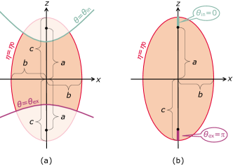
Figure 1(a) shows a conductor in the shape of a prolate ellipsoid with the long axis of length along the -axis. The conductor volume is parametrized by with arbitrary and in an ellipsoidal reference frame defined by
| (2) |
being the Cartesian coordinates. The ellipsoid has rotational symmetry—its cross-sections orthogonal to the -axis are circles. The largest circle is in , which is equivalent to , with the diameter . The length of the ellipsoid is . Thus, the aspect ratio (slimness) of the ellipsoid is . It becomes infinite for , . Then the ellipsoid degenerates to a straight line of length with its ends being the foci of the ellipsoid in . I call this the thin wire limit.
II.1 The Potential Inside the Ellipsoid and the Charge on the Contacts
Current flows between the hyperboloid coordinate surfaces and for and arbitrary . There, the potential is constant (Dirichlet boundary condition). The lateral surface of the truncated ellipsoid , , arbitrary , is insulating. There, the normal derivative of the potential vanishes (Neumann boundary condition). All boundary conditions do not depend on and , therefore the same applies to the potential, . For stationary current flow with uniform scalar conductivity the potential satisfies Laplace’s differential equation in ellipsoidal coordinates with the solution MoonSpencer
| (3) |
is a Legendre function of the second kind and of order zero. We define ground potential in , which means The constant is determined by the current flowing through the ellipsoid (Appendix A).
For the potential close to the -axis we write with . From (2) we know . Therefore small means either or or . Let us consider the case of ’small ’. There we have the full ellipsoid of Figure 1(b), and the contacts are the lines in the shape of infinitely thin needles of infinite conductivity. They are on the -axis, pushed into the ellipsoid until the tips of the needles reach the focus points. We enter with into (2),
| (4) |
Inserting this into (3) gives for
| (5) |
Applying Gauss’s electric flux theorem Gauss-theorem to on the contact gives the charge on the contact
| (6) |
With , , (conductivity of copper), and the elementary charge we find that there is only a single electron on the contact, regardless if the ellipsoid is very slim or not! Interestingly, the same tiny amount of surface charge sits in a ° bend in an ordinary wire with conductivity to guide the current around the corner Zangwill . Hence, a very small charge has a huge effect on the local electric field.
Irrespective of the slimness of the ellipsoid the potential at the contact of current injection in (5) is infinite, because the contact has zero diameter (it is a line). Contacts with infinite contact resistance are not unusual in electrical engineering—they occur for example in Van der Pauw’s measurement of the sheet resistance of thin plates with point or line contacts originalVdP and they also occur in Hall plates with point or line contacts Hall . If current is injected in such a contact, its potential rises unboundedly with a logarithmic singularity. A more surprizing finding is that in (5) the electric field on the contact and parallel to the contact does not vanish. This is a consequence of the fact that the potential at the contact is infinite, which means that it takes infinite energy to shuffle a small test charge from infinity onto the contact. Conversely, the electric field along the contact is only finite, and therefore we need only finite energy to shift this test charge along the contact.The finite energy needed to shift a test charge along the contact is still negligible against the infinite energy to bring it onto the contact, and in this asymptotic sense the contact is still an iso-potential surface. The radial field on the entire contact is infinite, see (5), and therefore the field lines of are perfectly perpendicular to the contact—in this respect the contact still behaves as we expect it from an ideal contact. Note that on the one hand the conductivity of the line contact is infinite, on the other hand its thickness is zero, and this may serve as an explanation for the line contact not being able to force zero tangential electric field. Note also that we cannot study this phenomenon by numerical simulation techniques like finite elements (FEM), because these programs cannot handle infinite quantities. They cannot represent infinite radial field on the line contact and therefore erroneously they assume zero tangential field to arrive at correct E-field lines orthogonal to the contacts.
The same phenomenon occurs in electrostatics, if we charge up an infinitely thin straight wire of finite length Jackson-revisited : The capacitance of such an ideal needle vanishes, see (22). Hence, it takes infinite energy to charge it. The charges distribute homogeneously on the ideal needle, yet they seem not to be in equilibrium, because there is a finite electric field acting on them in the direction of the needle. Again here the finite energy needed to shift a test charge along the ideal needle is negligible against the infinite energy needed to bring it onto the ideal needle, and the field lines are perfectly orthogonal to the ideal needle. Also here, standard FEM codes assume isopotential along the needle, thereby failing to predict the finite tangential electric field on the needle.
II.2 The Potential Outside the Ellipsoid and the Charge on the Ellipsoid
The general ansatz for the potential outside the full ellipsoid of Fig. 1(b) is
| (7) |
In (7) we have to discard the terms , because they are singular in and . This means . Indeed, the potential is singular in and , but only for , whereas it is regular for . Continuity of the potential at the surface means . Splitting up this identity into even and odd functions of gives
| (8) |
Thus, . For we multiply both sides with and integrate over . Note that are orthogonal Arfken-ortho , , but are not orthogonal. In Appendix B we prove
| (9) |
Using this in (8) finally gives
| (10) |
The electric field component perpendicular to the surface of the conductor is MoonSpencer3
| (11) |
where is the unit vector in the direction of growing (with and staying constant). In (11) we can further use
| (12) |
Conversely, , because the inside potential does not depend on , see (3). Therefore the charge density on the surface of the ellipsoid is equal to (Ref. Gauss-theorem, ).
The total charge on the surface of the ellipsoid in a ring of width at position is
| (13) |
where is the perimeter of the ring at position , and is the width of the ring in the direction tangentially to the surface of the ellipse. If the slimness of the ellipsoid gets infinite, it means and and and . In Appendix C we prove
| (14) |
With , we get for the line charge density of an infinitely slim ellipsoid
| (15) |
The infinite sum in (15) can be summed up, see Appendix D. With and , both valid for , we get
| (16) |
For the line charge density is linear in ,
| (17) |
which is identical to Ref. Assis1999b, for . If the wire becomes infinitely long, yet its diameter remains finite, the line charge density in (17) goes logarithmically to zero, which is also identical to Refs. Assis1999, and CombesLaue1980, . If the wire length is fixed and the diameter goes to zero, the line charge density grows unboundedly. The total charge in the upper half of the infinitely thin wire is
| (18) |
Therefore in the case of an infinitely thin resistive wire carrying DC-current, the net charge becomes infinite on the surface of the upper half of the wire. The reason for this singular behavior is that the voltage drop along the wire rises faster than the capacitance of the wire diminishes while the ellipsoid gets thinner. Note that the logarithimc singularity of in is not responsible for the net charge becoming infinite: If we use (17) instead of (16) in the integration of (18), the net charge is only times smaller. In particular the charge on the surface of the ellipsoid is much larger than the charge on the contact, . This is important, because it justifies the neglection of when we compute the electric force between two wires in the next section.
III The Electric Force between Two Infinitely Thin Resistive Wires with DC Currents
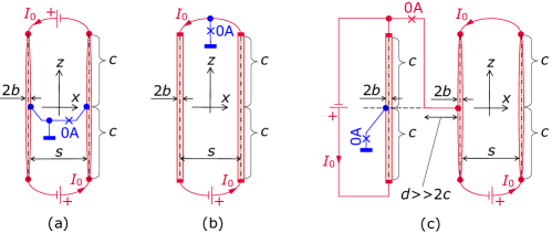
Let us consider two thin wires of finite lengths , both being parallel to the -axis and extending from to . Their cross-sections are circular, and their center lines are spaced apart by a distance . A DC-current flows in opposite directions through both wires. The wires are thought to be prolate ellipsoids with their thickest diameters in being . Let the wire diameter shrink infinitely, , which means and . The asymptotic limit of this process is identical to the thin wire limit of a cylindrical wire of constant diameter , which also tends to zero, . During this limit process the line contacts of the ellipsoids shrink to point contacts as , whereas the circular disk contacts at the end faces of the cylindrical wires also become point contacts as . For a finite diameter the resistance between the contacts of an elliptical wire is infinite (, see (3)), whereas the resistance of a cylindrical wire is finite, . However, in the thin wire limit both resistances are identical, , which means that the thinner the wires get the more similar their resistances become, although they both tend to infinity. Then the potentials along the wires, the electric field around them, the charges on them, and the forces between them converge to the very same limit. In the following we will see how the voltage between both wires and the choice of the common ground node affects the electric force.
III.1 Wires are grounded at their halves: Figure 2(a)
In this scenario a first current source is connected between the upper contacts of the wires, and a second identical current source is connected between their lower contacts (see Figure 2(a)). Both wires are grounded in . No current flows into the ground node due to the symmetry. Thus, the left wire has a line charge density from (16) and the right wire has a line charge density . Then the -component of the electric force on the line charge of the right wire is given by Coulomb’s force law Coulomblaw between two differential charges on the first and second wires, summed up over both wires,
| (19) |
This equation can be massaged into the following form (see Appendix E),
| (20) |
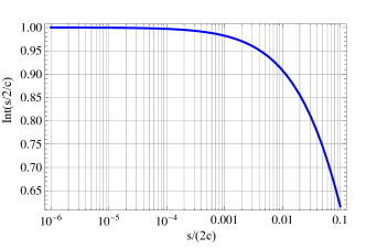
The negative sign of in (20) means that the electric force due to anti-parallel currents in both wires is attractive. Figure 3 shows a plot of . It is close to 1 if the wire spacing is less than 1% of the wire length. Then, the electrical force between both wires is dominated by the factors in front of . In particular, for small spacing the electrical force is proportional to , whereas for very large spacing, , the electric force is proportional to . For constant current the electric force grows unboundedly if the wire diameter diminishes.
For anti-parallel currents in both wires, the magnetic force on the right wire is given by the Lorentz law, with Vs/Am. The positive sign means repulsion. Finally, the ratio of electric over magnetic force is
| (21) |
wherein is the impedance of free space. The characteristic length is times the ratio of the wire resistivity over . For metal wires the resistivity in is much smaller than in , and therefore is very small (fractions of a nano-meter, for copper wires ). Consequently, the electric force is much smaller than the magnetic force, as long as the wire length is less than a few meters and the wire diameter is more than a tenth of a milli-meter (Table 1).
| # | for | ||||||
|---|---|---|---|---|---|---|---|
| with (21), Fig. 2(a) | with (24), Fig. 2(b) | ||||||
| 1 | 10 m | 0.1 mm | 1 cm | 3.95 mN | 3.14 A | -47.2 ppm | -99.2 ppm |
| 2 | 1 m | 0.1 mm | 1 cm | 395 N | 3.14 A | -0.692 ppm | -1.48 ppm |
| 3 | 1 m | 0.1 mm | 10 cm | 39.5 N | 3.14 A | -0.546 ppm | -1.34 ppm |
| 4 | 1 m | 1 mm | 10 cm | 0.395 N | 314 A | ||
| 5 | 0.5 m | 0.5 mm | 6 mm | 0.206 N | 78.5 A | ||
| 6 | 1 m | 1 m | 1 mm | N | 314 A | -33.08 | -70.24 |
| 7 | 1 m | 1 nm | 1 mm | N | 314 pA |
III.2 Wires are grounded at their upper ends: Figure 2(b)
Here we compute the electric force between the two cylindrical wires of Figure 2(b) in the limit . The striking difference to the preceding Section is that now the wires are shorted at their upper ends. In the thin wire limit the scenario in Figure 2(b) is equivalent to the scenario in Figure 2(c), which we use to compute the electric force. There the potential in the middle of the left elliptical wire is and in the thin wire limit the potential in the middle of the right elliptical wire is (because ). Thus, we may consider the potential in Scenario (c) as a linear superposition of the scenario in Figure 2(a) and an electrostatic scenario. In the electrostatic scenario no current flows through the ellipsoids, and they are charged up to . For the electric potentials it holds , where the indices ’, ’’ refer to the Figures 2(a),(c) and the index ’’ denotes the electrostatic case. The charges also add up analogously. The amount of charge needed to hold a prolate ellipsoid at potential is given by
| (22) |
whereby the capacitance of a prolate ellipsoid, , is derived in Appendix F. In the limit of an infinitely thin cylindrical wire it is known that the charge in electrostatic equilibrium () distributes uniformly on it Maxwell ; Andrews ; Jackson-revisited ; Jackson2 . Hence, the line charge density in the electrostatic case is with
| (23) |
If we add to in (16), we finally get the electric force between infinitely thin cylindrical wires in Figure 2(b)
| (24) |
Comparison of (24) with (20) shows that the electric force between infinitely thin wires grounded at their upper ends in Figure 2(b) is 2.2 times stronger than if the wires are grounded at their centers in Figure 2(a).
IV Electrostatic Induction between Both Wires
If the current carrying wires of length are brought at a distance , the surface charges on the first wire generate an electric field that acts on the second wire, and redistributes the charges there. So far, we have neglected this electrostatic induction, but here we want to estimate its order of magnitude. To this end we compare the electric field generated by the charges of a wire with the electric field generated by the charges of the other wire. Thereby we only need to consider , because in the thin wire limit the charges cannot move in lateral x-, y-directions.
generated by the charges of the first wire onto themselves:
In the thin wire limit we use with in (2). It gives and for .
Inserting this into (3) and differentiating against gives
| (25) |
In the limit of an infinitely thin wire we replace and and get
| (26) |
generated by the charges of one wire onto the other wire for the scenario in Figure 2(a):
| (27) |
This integral can be computed with Mathematica, but its exact formula is not even necessary if we pull out the diverging terms in for ,
| (28) |
This proves that the electric field acting on the charges of one wire produced by the charges on the other wire is infinitely smaller than the field of the charges on a wire on themselves, if both wires are infinitely thin while their spacing is finite. Therefore we can neglect electrostatic induction between both wires.
V Conclusion
In this paper I discussed the surface charges on an infinitely thin straight resistive wire which carries a DC-current. Thereby the wire is replaced by a prolate ellipsoid in the limit of infinite slimness. The distribution of surface charges varies linearly with the position near the center of the wire, whereas it has a logarithmic singularity at the ends of the wire. If two wires run parallel, electrostatic induction is negligible, as long as the wires are infinitely thin and spaced apart at a finite distance. The electric force between the surface charges on both wires was computed. It depends on the voltage drop along the wires, on the voltage between both wires, on the wire lengths, diameters, and their spacing. If the current, the wires lengths, and their spacing are fixed while the wires diameters shrink, the voltage drop grows unboundedly, and this will give infinite surface charges and infinite electric force. This limit leads to infinite current density and heating in the wire, which eventually distroys the wire. However, if we consider the ratio of electric over magnetic force between both wires, this ratio is independent of the current, and we may scale down the current synchronously with the wire diameter to achieve constant current density during the limit process. Of course, the magnetic force decreases with the current accordingly, but in practice this just calls for a sufficiently sensitive method of force measurement. In such a scenario the electric force can indeed become even stronger than the magnetic force.
The electric force can be eliminated if each wire is surrounded by an electric shield (like a coaxial cable) and both shields are tied to the same potential (e.g. ground). Each shield has to be clamped mechanically to its conductor, because there might be an electric force between the shield and its conductor (depending on symmetry).
This manuscript was submitted to the American Journal of Physics, but it was rejected (too long, too mathematically dense, lack of interest).
The author has no conflicts to disclose.
Appendix A How to determine the constant of the potential
Let us look at the potential close to , which means with and with . Inserting this into (2) gives
| (29) |
With the radial distance it follows with (29)
| (30) |
We solve (30) for , whereby and have opposite sign. Inserting this into (3) gives
| (31) |
From (31) we get the -component of the electric field in
| (32) |
With Ohm’s law the -component of the current density is , and the total current downward through the ellipsoid is given by the integral
| (33) |
Here we used . Inserting from (33) into (3) gives the potential everywhere inside the ellipsoid, if the current is known.
Appendix B Proof of (9)
| (34) |
where we first developped the logarithm into a Taylor series, and then we used the Legendre series/sum of odd powers of from Ref. Arfken2, . Next we apply the orthogonality of the Legendre polynomials on (34), , and we reverse the sequence of summations, . Then (34) becomes
| (35) |
The summation in (35) is handled by Mathematica. For its proof we start with the following identity Arfken5
| (36) |
Integration of (36) gives
| (37) |
With the recurrence relation Arfken6
| (38) |
it follows for
| (39) |
In (38,39) the primes denote differentiation with respect to . We insert (45) into (39), let , and insert this into (37),
| (40) |
Inserting (49) and (51) into (40) finally gives
| (41) |
Appendix C Proof of (14)
With Mathematica we compute
| (42) |
For a proof we start with the recurrence relation Arfken6 ; Hobson1
| (43) |
with the limits of the first three Q-functions
| (44) |
Inserting (44) into (43) shows that the logarithmic term is identical for all . Thus, we can write
| (45) |
where is a rational number. We insert (45) into the recurrence relation (43) and get
| (46) |
Inserting (46) into the left side of (42) gives
| (47) |
If we express by via the recurrence relations (46) we get after a few re-arrangements
| (48) |
For the first few indices this gives
| (49) |
Appendix D How to compute the sum in (15)
We want to compute
| (52) |
For the sum we start with the generating function of the Legendre polynomials Arfken4
| (53) |
We integrate (53) once over and once over . Adding both results cancels out even indices ,
| (54) |
For the sum we set in (53) and divide both sides by . This gives
| (55) |
Like above, we integrate (55) once over and once over , and we add both results to cancel out even indices ,
| (56) |
Next, we integrate (56) over whereby we take the Cauchy principal value around the singularity in ,
| (57) |
The computation of the integrals in (57) is easier, if one starts with the integration over before the integration over ,
| (58) |
Appendix E How to derive in equation (20)
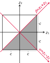
Let us call the integrand in the last line of (19) . It is symmetrical, because it is identical to . Therefore, we may halve the integration domain in (19),
| (59) |
In Figure 4 this reduces the integration domain from the square to the dark triangle. Next, we transform the integration variables according to
| (60) |
which is also shown in Figure 4. Thereby the differential surface elements relate via the Jacobian determinant,
| (61) |
It holds
| (62) |
is an even function of . Therefore, in (62) the two integrals over are identical, and the final result is given in (20), whereby we used the transformations and . In (20) the integration over can be done in closed form,
| (63) |
with the imaginary unit , and with the poly-logarithm . is real, all imaginary portions are in the last line of (63) and cancel out.
We compute the limit of for with partial integration,
| (64) |
For the integral on the right hand side of in (64) we get again with partial integration
| (65) |
For , the integral in (65) tends to (computed with Mathematica). We re-insert this into (65) and (64), and compute with Mathematica the limit for . The result is .
Appendix F The Capacitance of a Prolate Ellipsoid
The potential outside a charged metallic ellipsoid has the same ansatz as in (7) with the only non-zero coefficient , whereby the ellipsoid is at potential and its surface has the ellipsoidal coordinate . The electric field on the surface of the ellipsoid is given analogous to (11),
| (66) |
The charge on this ellipsoid is given analogous to (13)
| (67) |
We insert into (67) and compute , which gives from (22), which is consistent to Refs. Kottler, ; Smythe, ; Stratton2, .
References
-
(1)
Richard Becker. Theorie der Elektrizität. Volume I: Einführung in die Maxwellsche Theorie (Teubner Verlag, Stuttgart 1973), 21st edition, chapter 5.4 (in German) also available in English:
Richard Becker. Electromagnetic Fields and Interactions. Volume I: Electromagnetic Theory and Relativity (Blaisdell, New York 1964) - (2) John David Jackson. Classical Electrodynamics. (Walter de Gruyter, Berlin 1983), 2nd edition, Appendix. Units and Dimensions
- (3) Erik Hallén. Electromagnetic Theory. (John Wiley and Sons, New York 1962), chapter 11.1
-
(4)
Károly Simonyi. Theoretische Elektrotechnik. (VEB Deutscher Verlag der Wissenschaften, Berlin 1971), 4th edition, chapter 1.11 (in German) also available in English:
K. Simonyi. Foundations of Electrical Engineering: Fields—Networks—Waves. (Elsevier 2016). - (5) Hellmut Hofmann. Das elektromagnetische Feld. (Springer Verlag, Wien 1986), 3rd edition, §3.3.2.1.8 (in German)
-
(6)
Günther Lehner. Elektromagnetische Feldtheorie. (Springer, Heidelberg 2010), 7. edition, chapter 1.13 (in German)
Günther Lehner, G. Electromagnetic field theory for engineers and physicists. (Springer Science & Business Media 2010). - (7) H. Nakamura, H. “A Servo-Controlled Balance for the Absolute Ampere Determination,” Japanese Journal of Applied Physics, 17(8), 1397 (1978).
- (8) I. A. Robinson and S. Schlamminger. “The watt or Kibble balance: a technique for implementing the new SI definition of the unit of mass,” Metrologia, 53 (5), A46 (2016).
- (9) S. Schlamminger and D. Haddad. “The Kibble balance and the kilogram” Comptes Rendus Physique 20.1-2, 55-63 (2019).
-
(10)
A. K. T. Assis and A. J. Mania. “Surface charges and electric field in a two-wire resistive transmission line,” Revista Brasileira de Ensino de Física 21 (4), 469-475 (1999).
In eq.(14) a factor is missing in the denominator. Moreover, eq.(10) is not consistent with eq.(12) in Ref. Assis1999, by the same authors, because in eq.(10) the line charge is reciprocal to , yet it should be reciprocal to (in our notation). Also in eq.(14) should be replaced by . - (11) A. Marcus. “The electric field associated with a steady current in long cylindrical conductor,” American Journal of Physics 9 (4), 225-226 (1941).
- (12) Julius Adams Stratton. Electromagnetic Theory. (McGraw-Hill, New York, 1941), §4.21, problem 2.
- (13) E. Merzbacher. “A puzzle from professor Eugen Merzbacher,” Am. J. Phys 48, 178 (1980).
- (14) J. D. Jackson. “Surface charges on circuit wires and resistors play three roles,” American Journal of Physics, 64 (7), 855-870 (1996).
- (15) A. K. T. Assis, W. A. Rodrigues Jr, and A. J. Mania. “The electric field outside a stationary resistive wire carrying a constant current,” Foundations of Physics 29 (5), 729-753 (1999).
- (16) Andre Koch Torres Assis, and Julio Akashi Hernandes, The electric force of a current: Weber and the surface charges of resististive conductors carrying steady currents, 1st edition (Apeiron, Montreal, Canada, 2007).
- (17) Andrew Zangwill, Modern Electrodynamics, 1st edition (Cambridge Univ. Press, Cambridge, UK, 2013), chapter 9.7.4.
- (18) J. C. Maxwell, “On the electrical capacity of a long narrow cylinder, and of a disk of sensible thickness,” Proc. London Math. Soc. IX, 94-101 (1878).
- (19) M. Andrews, “Equilibrium charge density on a conducting needle,” American Journal of Physics 65 (9), 846-850 (1997).
- (20) J. D. Jackson. “Charge density on thin straight wire, revisited,” American Journal of Physics 68.9 (2000): 789-799.
- (21) Parry Moon and Domina Eberle Spencer, Field Theory for Engineers, 1st edition (D. van Nostrand Company Inc., Princeton, New Jersey, 1961), §9.02, eqs. (9.12), (9.13).
- (22) William Ralph Smythe. Static and Dynamic Electricity, 3rd ed., (Taylor & Francis, 1989) chapter I, 1.10 (1).
- (23) L. J. van der Pauw. “A method of measuring the resistivity and Hall coefficient on lamellae of arbitrary shape,” Philips technical review 20, 220-224 (1958).
- (24) M. G. Buehler, and G. L. Pearson. “Magnetoconductive correction factors for an isotropic Hall plate with point sources,” Solid-State Electronics 9 (5), 395-407 (1966).
- (25) George Arfken. Mathematical Methods for Physicists, 3rd edition (Academic Press Inc., Boston 1985), chapter 12.3.
- (26) see Ref. MoonSpencer, , §9.02.
- (27) see Ref. MoonSpencer, , §9.06, after eq. (9.32).
- (28) see Ref. Assis1999, , eq.(12). Note that eq.(12) has a typo: the denominator should be multiplied by the wire length—compare with eq.(16) there.
- (29) C. A. Coombes, and H. Laue. “Electric fields and charges distributions associated with steady currents,” Am. J. Phys 49 (5), 450, eq.(8) (1981).
- (30) see Ref. Stratton1941, , Chapter III, Section 3.6.
- (31) see Ref. Arfken-ortho, , exercise 12.4.6(b).
- (32) see Ref. Arfken-ortho, , eq.(12.20).
- (33) J. D. Jackson, “Charge density on a thin straight wire: The first visit,” American Journal of Physics, 70 (4), 409-410 (2002).
- (34) see Ref. Arfken-ortho, , exercise (12.10.4).
- (35) see Ref. Arfken-ortho, , exercise (12.10.5).
- (36) Ernest William Hobson. The Theory of Spherical and Ellipsoidal Harmonics, (Chelsea Pub., N.Y. 1965), chapter II, 42., (70).
- (37) Friedrich Kottler. “Elektrostatik der Leiter,” in Handbuch der Physik, (Springer Verlag, Berlin, 1927) vol. XII, chapter 4, paragraph 88, (94a). (in German)
- (38) see Ref. Gauss-theorem, , chapter V, 5.02 (4).
- (39) see Ref. Stratton1941, , Chapter III, Section 3.26, eq.(14).