Cosmic Expansion and Noether Gauge Symmetries in $f(R,T,R_{\mu\nu}T^{\mu\nu})$ Gravity

Abstract

The present work explores different evolutionary phases of isotropically homogeneous and flat cosmos filled with dust fluid in non-minimally coupled gravity. We consider different models of this gravity to discuss the presence of symmetry generators together with conserved integrals using Nother Gauge symmetry scheme. In most of the cases, we obtain temporal and scaling symmetries that yield conservation of energy and linear momentum, respectively. In the absence of contracted Ricci and energy-momentum tensors, we obtain maximum symmetries but none of them correspond to any standard symmetry or conservation law. We formulate exact solutions and construct graphical analysis of standard cosmological parameters. We observe realistic nature of new models via squared speed of sound, viability conditions suggested by Dolgov-Kawasaki instability and state-finder parameters. We investigate the behavior of fractional densities and check the compatibility with Planck 2018 observational data. The new models are stable and viable preserving compatibility with $\Lambda$CDM and Chaplygin gas models. It is concluded that most of the solutions favor accelerated cosmic expansion.

Keywords: Noether symmetry; Exact solution; $f(R,T,R_{\mu\nu}T^{\mu\nu})$ gravity.
PACS: 04.20.Jb; 04.50.Kd; 95.36.+x.

1 Introduction

The primal facts and observational evidences reveal that the cosmos encounters an exponential expansion at the very early stage. This phase of the universe leads to current accelerated expansion by following radiation and matter dominated phases. Such variations in cosmos trigger cosmologists to understand matter distribution and find possible reasons behind these expanding phases of the universe. The most compatible explanation is the existence of some exotic fluid incorporating negative pressure that induces strong anti-gravitational effects and defines current cosmic expansion. The origin as well as striking nature of this anti-gravitational force is yet unknown and consequently, named as dark energy (DE). At theoretical scales, there are different approaches to deal with intriguing nature of DE such as modifying Einstein-Hilbert action that leads to develop modified theories of gravity and dynamical DE models. The advancements in gravitational part of Einstein-Hilbert action define higher order minimally as well as non-minimally coupled gravitational theories, i.e., $f(R)$, $f(R,T)$ and $f(R,T,R_{\mu\nu}T^{\mu\nu})$ ($R_{\mu\nu}$, $T^{\mu\nu}$, $R$ and $T$, represent the Ricci and energy-momentum tensors with their traces, respectively) theories. The impact of minimal coupling between curvature and matter variables yields intriguing phenomenologies and solution to many cosmological problems [1].

The revolutionary idea of introducing non-minimal interactions between geometric and matter contents put forward fascinating approaches to investigate different cosmological scenarios and current state of cosmos. Bertolami et al. [2] proposed a generic function admitting non-minimal interactions between scalar curvature and matter Lagrangian. Harko et al. [3] extended this non-minimal coupling by replacing matter Lagrangian with trace of the energy-momentum tensor, referred to as $f(R,T)$ theory. Such advancements not only deal with cosmic evolution and current expansion but also suggest efficient approaches to study dark matter in galaxies, natural conditions for early universe and existence of feasible cosmological configurations [4]. Sharif and Zubair [5] followed this idea of non-minimal coupling to interpret thermodynamical picture, stability criteria, reconstruction of some new DE models and exact solutions of isotropic/anisotropic cosmological models.

In the presence of electromagnetic field, the non-minimal interactions between geometric and matter variables identically disappear from the field equations of $f(R,T)$ gravity for $T=0$ and recovers $f(R)$ gravity. This aspect motivates to introduce a generalized version of $f(R,T)$ theory by taking into account non-minimal coupling between contracted Ricci and energy-momentum tensors known as $f(R,T,R_{\mu\nu}T^{\mu\nu})$ gravitational theory [6]. Unlike $f(R,T)$ theory, the extended version preserves coupling of electromagnetic field with contracted Ricci and energy-momentum tensors for $T=0$ [7]. In non-minimally coupled theories, the energy-momentum tensor remains non-conserved due to the presence of an extra force that deviates massive test particles and also introduce instabilities against local perturbations. Using Dolgov-Kawasaki instability criteria, some constraints are introduced whose viability eliminates these instabilities [8]. Sharif and Zubair [9] discussed thermodynamical laws and viability of energy constraints for different cosmological models. Different cosmological aspects like gravitational collapse, dynamical instability, cosmic evolution and exact solutions for self-gravitating objects are significantly studied in the frame-work of $f(R,T,R_{\mu\nu}T^{\mu\nu})$ gravity [10].

In minimally/non-minimally coupled gravitational theories, the exact solutions to the non-linear field equations come up with significant approaches to understand cosmic evolution, configurations and matter contributions. Sebastiani and Zerbini [11] formulated non-trivial exact solutions for static spherically symmetric structure in $f(R)$ gravity. In the presence of scalar field, Maharaj et al. [12] found solutions corresponding to de Sitter, oscillating, accelerating, decelerating and contracting cosmos in the same gravity. Sharif and Zubair [13] determined solutions for power-law and exponential anisotropic cosmological models in $f(R,T)$ theory. Harko and Lake [14] calculated exact solutions to discuss the effect of non-minimal coupling between scalar curvature and matter Lagrangian on cylindrical model. Shamir and Raza [15] obtained two solutions characterizing cosmic string and non-null electromagnetic field in the background of $f(R,T)$ gravity. Shamir [16] found three unique solutions for Bianchi I universe model and discussed their physical behavior via cosmological parameters in the same gravity.

The technique of Noether symmetry puts forward an interesting way to identify symmetries and relative conserved entities of cosmological systems. This approach significantly reduces the complexity of non-linear higher order partial differential equations and yield corresponding exact solutions. The existence of symmetries and conservation laws enhance physical worth of modified theories as if a theory does not incorporate any symmetry or conserved quantity then it may refer to as nonphysical theory. Capozziello et al. [17] considered constant Ricci scalar and power-law $f(R)$ model to find exact solutions for static spherically symmetric metric using Noether symmetry technique. Hussain et al. [18] evaluated Noether point symmetries of flat FRW metric with same $f(R)$ model and zero boundary term. Shamir et al. [19] extended their work for non-zero boundary term and obtained some extra symmetries.

Atazadeh and Darabi [20] followed this technique to reconstruct viable $f(\mathrm{T})$ models ($\mathrm{T}$ represents torsion) that corresponds to power-law expansion. Momeni et al. [21] solved over determining system of mimetic $f(R)$ gravity to get Noether point symmetry together with conserved charge whereas they found power-law solution that explains decelerating cosmic expansion in $f(R,T)$ theory. Sharif and Fatima [22] established symmetry generators and conserved entities for both vacuum as well as non-vacuum flat isotropic homogeneous cosmological model in $f(\mathcal{G})$ gravity ($\mathcal{G}$, referred to Gauss-Bonnet invariant). We have discussed the existence of Noether symmetries with conserved quantities and evaluated some exact solutions of anisotropic universe model in the background of $f(R)$ and $f(R,T)$ theories [23]. Besides cosmological evolution and current expansion, we have also studied cosmological configurations like wormhole whose stability as well as viability is examined via constant and variable red-shift functions in both theories [24]. Sharif et al. [25] established some realistic and viable wormholes for both exponential as well as quadratic $f(\mathcal{G})$ models.

Motivated from above significant outcomes and growing interest in cosmological aspects, it would be interesting to study cosmic expansion and evolution in the background of non-minimally coupled $f(R,T,R_{\mu\nu}T^{\mu\nu})$ theory. In this paper, we consider flat isotropic dust cosmological model to evaluate Noether point symmetries, conserved integrals and some solutions using Noether Gauge symmetry scheme. We construct graphical analysis of standard cosmological parameters and fractional densities. To study model feasibility, we also investigate the behavior of squared speed of sound, viability constraints and state-finder parameters. The format of the paper is given as follows. In section 2, we discuss basic formulation of $f(R,T,R_{\mu\nu}T^{\mu\nu})$ gravity and Noether gauge symmetry scheme. In sections 3-6, we obtain Noether gauge symmetries, conserved quantities and exact solutions. Furthermore, we establish cosmological analysis via standard cosmological parameters and corresponding graphical illustration. In the last section, we provide a summary of our results.

2 $f(R,T,R_{\mu\nu}T^{\mu\nu})$ Gravity and Noether Gauge Symmetry Approach

For non-minimally interacting curvature and matter variables, the action of this gravity is defined as [6]

$$\mathcal{I}=\frac{1}{2\kappa^{2}}\int d^{4}x\sqrt{-g}[f(R,T,R_{\mu\nu}T^{\mu\nu})+\mathcal{L}_{m}],$$ (1)

where $f$ represents a generic function inducing non-minimal coupling between scalar curvature, matter and contracted Ricci and energy-momentum tensors while $\kappa$, $g$ and $\mathcal{L}_{m}$ describe coupling constant, determinant of the metric tensor ($g_{\mu\nu}$) and Lagrangian relative to ordinary matter, respectively. For the sake of simplicity, we consider $R_{\mu\nu}T^{\mu\nu}=Q$. The matter Lagrangian depending on the metric tensor leads to the following form of the energy-momentum tensor

$$T_{\mu\nu}=-\frac{2}{\sqrt{-g}}\frac{\delta(\sqrt{-g}\mathcal{L}_{m})}{\delta g^{\mu\nu}}=g_{\mu\nu}\mathcal{L}_{m}-\frac{2\delta\mathcal{L}_{m}}{\delta g^{\mu\nu}}.$$ (2)

For $\kappa^{2}=1$, the variation of action (1) with respect to the metric tensor yields non-linear partial differential field equation as follows

$$(f_{{}_{R}}-f_{{}_{Q}}\mathcal{L}_{m})G_{\mu\nu}+\left[\Box f_{{}_{R}}+\frac{1}{2}Rf_{{}_{R}}-\frac{1}{2}f+f_{{}_{T}}\mathcal{L}_{m}+\frac{1}{2}\nabla_{\alpha}\nabla_{\beta}\left(f_{{}_{Q}}T^{\alpha\beta}\right)\right]g_{\mu\nu}$$

$$-\nabla_{\mu}\nabla_{\nu}f_{{}_{R}}+\frac{1}{2}\Box(f_{{}_{Q}}T_{\mu\nu})+2f_{{}_{Q}}R_{\alpha(\mu}T_{\nu)}^{\alpha}-\nabla_{\alpha}\nabla_{(\mu}[T_{\nu)}^{\alpha}f_{{}_{Q}}]-2(f_{{}_{T}}g^{\alpha\beta}$$

$$+f_{{}_{Q}}R^{\alpha\beta})\frac{\partial^{2}\mathcal{L}_{m}}{\partial g^{\mu\nu}\partial g^{\alpha\beta}}=(1+f_{{}_{T}}+\frac{1}{2}Rf_{{}_{Q}})T_{\mu\nu}.$$ (3)

Here $G_{\mu\nu}$ identifies as the Einstein tensor, $\nabla_{\mu}$ defines covariant derivative, $\Box=\nabla_{\mu}\nabla^{\mu}$ whereas $f_{{}_{R}},~{}f_{{}_{T}}$ and $f_{{}_{Q}}$ denote derivative of the generic function corresponding to $R,~{}T$ and $Q$, respectively.

The equivalent form of the above field equations to the Einstein field equations is given by

$$G_{\mu\nu}=R_{\mu\nu}-\frac{1}{2}Rg_{\mu\nu}=T_{\mu\nu}^{eff},$$ (4)

where the effective energy-momentum tensor $T_{\mu\nu}^{eff}$ incorporates matter and higher order curvature terms given as

$$T_{\mu\nu}^{eff} = \frac{1}{f_{{}_{R}}-f_{{}_{Q}}\mathcal{L}_{m}}[(1+f_{{}_{T}}+\frac{1}{2}Rf_{{}_{Q}})T_{\mu\nu}+\{\frac{1}{2}(f-Rf_{{}_{R}})-\mathcal{L}_{m}f_{{}_{T}}$$ (5)

$$- \frac{1}{2}\nabla_{\alpha}\nabla_{\beta}(f_{{}_{Q}}T^{\alpha\beta})\}g_{\mu\nu}-(g_{\mu\nu}\Box-\nabla_{\mu}\nabla_{\nu})f_{{}_{R}}-\frac{1}{2}\Box(f_{{}_{Q}}T_{\mu\nu})$$

$$+ \nabla_{\alpha}\nabla_{(\mu}[T_{\nu)}^{\alpha}f_{{}_{Q}}]-2f_{{}_{Q}}R_{\alpha(\mu}T_{\nu)}^{\alpha}+2(f_{{}_{T}}g^{\alpha\beta}+f_{{}_{Q}}R^{\alpha\beta})\frac{\partial^{2}\mathcal{L}_{m}}{\partial g^{\mu\nu}\partial g^{\alpha\beta}}].$$

The contraction of Eq.(3) relative to the metric tensor leads to construct a correspondence between trace of geometric and matter parts as follows

$$(f_{{}_{R}}+f_{{}_{Q}}\mathcal{L}_{m})R+\nabla_{\alpha}\nabla_{\beta}(f_{{}_{Q}}T^{\alpha\beta})+4f_{{}_{T}}\mathcal{L}_{m}-2f+3\Box f_{{}_{R}}+\frac{1}{2}\Box(f_{{}_{Q}}T)$$

$$+2f_{{}_{Q}}R_{\alpha\beta}T^{\alpha\beta}-2g^{\mu\nu}(f_{{}_{T}}g^{\alpha\beta}+f_{{}_{Q}}R^{\alpha\beta})\frac{\partial^{2}\mathcal{L}_{m}}{\partial g^{\mu\nu}\partial g^{\alpha\beta}}=(1+f_{{}_{T}}+\frac{1}{2}Rf_{{}_{Q}})T.$$

In the presence of non-minimal curvature-matter interactions, the covariant derivative of Eq.(3) fails to satisfy conservation of the energy-momentum tensor yielding

$$\nabla^{\mu}T_{\mu\nu}=\frac{1}{1+f_{{}_{T}}+(Rf_{{}_{Q}})/2}\left[\nabla_{\mu}(f_{{}_{Q}}T_{\sigma\nu}R^{\sigma\mu})-\frac{1}{2}(f_{{}_{Q}}f_{{}_{T}}R_{\alpha\beta}g_{\alpha\beta})\nabla_{\nu}T^{\alpha\beta}\right.$$

$$\left.+\nabla_{\nu}(\mathcal{L}_{m}f_{{}_{T}})-G_{\mu\nu}\nabla^{\mu}(f_{{}_{Q}}\mathcal{L}_{m})-\frac{1}{2}(\nabla^{\mu}(Rf_{{}_{Q}})+2\nabla^{\mu}f_{{}_{T}})T_{\mu\nu}\right].$$

The non-conserved energy-momentum tensor introduces an extra force given by

$$\frac{d^{2}x^{\alpha}}{ds^{2}}+\Gamma^{\alpha}_{\mu\nu}u^{\mu}u^{\nu}=\mathcal{F}^{\alpha},$$

where ${F}^{\alpha}$ defines extra force orthogonal to four velocity of the massive particles. In $f(R,T,Q)$ theory, it becomes

$$\mathcal{F}^{\alpha}=\frac{h^{\alpha\beta}}{(\rho_{m}+p_{m})(1+2f_{T}+Rf_{{}_{RT}})}[(f_{T}+Rf_{{}_{RT}})\nabla_{\beta}\rho_{m}-(1+3f_{T})\nabla_{\beta}p_{m}$$

$$-(\rho_{m}+p_{m})f_{{}_{RT}}R^{\gamma\delta}(\nabla\beta h_{\gamma\delta}-2\nabla\delta h_{\gamma\beta})-f_{{}_{RT}}R_{\gamma\delta}h^{\gamma\delta}\nabla_{\beta}(\rho_{m}+p_{m})].$$

The minimally coupled gravitational theories are strongly supported by the equivalence principle as it passes solar system tests in weak gravitational fields whereas non-minimally coupled theories incorporate an additional force that explicitly violates this principle. Recent observations of Abell Cluster A586 claim that violation of the equivalence principle is not the only criteria to rule out any gravitational theory as the equivalence principle test is constrained under the influence of weak gravitational force and results may vary in the presence of strong gravitational fields or interactions of DE or DM [26]. In modified theories of gravity, the matter Lagrangian plays a significant role to study conserved/non-conserved nature of matter. Different choices of matter Lagrangian interacting with curvature invariant lead to investigate the impact of geodesic as well as non-geodesic motion that unravel different cosmological issues and also elaborate physical constraints of a theory. In $f(R,\mathcal{L}_{m})$ theory, the additional force vanishes for $\mathcal{L}_{m}=p_{m}$ [27]. In $f(R,T)$ theory, the geodesic lines of motion are followed for perfect fluid distribution with $f_{T}(R,T)=0$ whereas the effect of extra force can be neglected in the presence of dust particles even with $f_{T}(R,T)\neq 0$. In $f(R,T,Q)$ theory, the additional force cannot be avoided even for dust particles or any particular choice of matter Lagrangian due to explicit dependence on the Ricci tensor. This dependence helps to explore evolutionary phases of cosmic regimes with strong curvature. The effect of non-geodesic particles can be ignored only for non-interacting curvature and matter variables, i.e., $f_{T}(R,T)=f_{{}_{RT}}=0$ [3].

The ordinary matter of cosmos is assumed to be distributed with perfect fluid whose energy-momentum takes the form

$$T_{\mu\nu}=(\rho_{m}+p_{m})v_{\mu}v_{\nu}+p_{m}g_{\mu\nu},\quad v_{\mu}=(-1,0,0,0),$$

where $\rho_{m}$ and $p_{m}$ refer to energy density and pressure, respectively whereas $v_{\mu}$ describes four velocity of the ordinary matter. The non-conserved nature of matter is independent of matter Lagrangian as the extra force does not disappear even for $\mathcal{L}_{m}=p_{m}$ or $\mathcal{L}_{m}=-\rho_{m}$. Therefore, the selection of matter Lagrangian is not unique and we consider $\mathcal{L}_{m}=-\rho_{m}$ for perfect fluid distribution.

For isotropic and homogenous flat cosmos, the cosmological model is described as

$$ds^{2}=-dt^{2}+a^{2}(t)(dx^{2}+dy^{2}+dz^{2}),$$ (6)

where the scale factor $a(t)$ represents cosmic expansion along $x,~{}y$ and $z$-directions. In order to construct point-like Lagrangian for the action (1), we use Lagrange multiplier approach leading to the following form

$$\mathcal{I} = \int\sqrt{-g}[f(R,T,Q)-\zeta(R-\bar{R})-\eta(T-\bar{T})-\vartheta(Q-\bar{Q})+\rho_{m}(a)]dt,$$

$$\bar{R} = 6\left(\frac{\ddot{a}}{a}+\frac{\dot{a}^{2}}{a^{2}}\right),\quad\bar{T}=3p_{m}-\rho_{m},\quad Q=-\frac{3\ddot{a}\rho_{m}}{a}+\frac{3p_{m}}{a^{2}}\left(2\dot{a}^{2}+a\ddot{a}\right).$$ (7)

Here $\sqrt{-g}=a^{3}$, $\zeta,~{}\eta$ and $\vartheta$ are scalar curvature terms whereas $\bar{R},~{}\bar{T}$ and $\bar{Q}$ refer to dynamical constraint. Varying the above action relative to $R,~{}T$ and $Q$, we obtain $\zeta=f_{{}_{R}},~{}\eta=f_{{}_{T}}$ and $\vartheta=f_{{}_{Q}}$ while integrating the second order derivatives in Eq.(7) leads to the following Lagrangian

$$\mathcal{L}(a,R,T,Q,\dot{a},\dot{R},\dot{T},\dot{Q})=a^{3}[f(R,T,Q)-Rf_{{}_{R}}-Tf_{{}_{T}}-Qf_{{}_{Q}}-(\rho_{m}-3p_{m})$$

$$\times f_{{}_{T}}-\rho_{m}]-6a\dot{a}^{2}f_{{}_{R}}-6a^{2}\dot{a}\dot{R}f_{{}_{RR}}-6a^{2}\dot{a}\dot{T}f_{{}_{RT}}-6a^{2}\dot{a}\dot{Q}f_{{}_{RQ}}+3a\dot{a}^{2}f_{{}_{Q}}(2\rho_{m}$$

$$-ap_{m}^{\prime}+a\rho_{m}^{\prime})+3a^{2}\dot{a}(\rho_{m}-p_{m})[\dot{R}f_{{}_{RQ}}+\dot{T}f_{{}_{TQ}}+\dot{Q}f_{{}_{QQ}}],$$ (8)

In a dynamical system, Hamiltonian equation interprets the total energy of a system while equation of motion is measured through Lagrange equation. Mathematically, these equations are defined as

$$\mathcal{H}=\Sigma_{i}\dot{q}^{i}p_{i}-\mathcal{L},\quad\frac{\partial\mathcal{L}}{\partial q^{i}}-\frac{d}{dt}\left(\frac{\partial\mathcal{L}}{\partial\dot{q}^{i}}\right)=0,$$

where $q^{i},~{}\dot{q}^{i}$ and $p^{i}$ describe generalized co-ordinates, velocity and momentum, respectively. For Eq.(8), the Hamiltonian equation is

$$\mathcal{H} = -\frac{3\dot{a}^{2}}{a^{2}}+\frac{1}{2(f_{{}_{R}}-\rho_{m}f_{{}_{Q}})}\left[f(R,T,Q)-Rf_{{}_{R}}-Tf_{{}_{T}}-f_{T}(\rho_{m}-3p_{m})\right.$$ (9)

$$+ \rho_{m}-Qf_{{}_{Q}}+\left.3\dot{a}H(\rho_{m}^{\prime}-p_{m}^{\prime})f_{{}_{Q}}+3H(\rho_{m}-p_{m})\{\dot{R}f_{{}_{RQ}}+\dot{T}f_{{}_{TQ}}+\dot{Q}f_{{}_{QQ}}\}\right.$$

$$- \left.6H\{\dot{R}f_{{}_{RR}}+\dot{T}f_{{}_{RT}}+\dot{Q}f_{{}_{RQ}}\}\right].$$

The Hamiltonian equation is also used to evaluate total energy density of the dynamical system for constraint $\mathcal{H}=0$. For generalized co-ordinates $q_{i}=\{a,R,T,Q\}$ and corresponding Lagrangian (8), the equations of motion turn out to be

$$\dot{a^{2}}+2a\ddot{a}+\frac{a^{2}}{2(f_{{}_{R}}-\rho_{m}f_{{}_{Q}})}\left[f(R,T,Q)-Rf_{{}_{R}}-Tf_{{}_{T}}-Qf_{{}_{Q}}-f_{T}(\rho_{m}-3p_{m})\right.$$

$$-\left.\rho_{m}-\frac{a}{3}(f_{T}(\rho_{m}^{\prime}-3p_{m}^{\prime})+\rho_{m}^{\prime})+2H\{2\dot{f}_{{}_{R}}-\dot{f}_{{}_{Q}}(2\rho_{m}+a\rho_{m}^{\prime}-ap_{m}^{\prime})\}\right.$$

$$+\left.2(\ddot{R}f_{{}_{RR}}+\ddot{T}f_{{}_{RT}}+\ddot{Q}f_{{}_{RQ}}+\dot{R}\dot{f}_{{}_{RR}}++\dot{T}\dot{f}_{{}_{RT}}+\dot{Q}\dot{f}_{{}_{RQ}})+(\ddot{a}+2aH^{2})\right.$$

$$\times\left.(\rho_{m}^{\prime}-p_{m}^{\prime})f_{{}_{Q}}-aH^{2}f_{{}_{Q}}(6\rho_{m}^{\prime}-2p_{m}^{\prime}+a\rho_{m}^{\prime\prime}-ap_{m}^{\prime\prime})+(\rho_{m}-p_{m})\right.$$

$$\times\left.(\ddot{R}f_{{}_{RQ}}+\ddot{T}f_{{}_{TQ}}+\ddot{Q}f_{{}_{QQ}}+\dot{R}\dot{f}_{{}_{RQ}}+\dot{T}\dot{f}_{{}_{TQ}}+\dot{Q}\dot{f}_{{}_{QQ}})\right]=0,$$ (10)

$$-a^{3}(Rf_{{}_{RR}}+Tf_{{}_{RT}}+Qf_{{}_{RQ}}+f_{{}_{RT}}(\rho_{m}-3p_{m}))+6a\dot{a}^{2}(f_{{}_{RR}}+\rho_{m}f_{{}_{RQ}})$$

$$+6a^{2}\ddot{a}f_{{}_{RR}}-3af_{{}_{RQ}}(\rho_{m}-p_{m})(2\dot{a}^{2}+a\ddot{a})=0,$$ (11)

$$-a^{3}(Rf_{{}_{RT}}+Tf_{{}_{TT}}+Qf_{{}_{TQ}}+f_{{}_{TT}}(\rho_{m}-3p_{m}))+6a\dot{a}^{2}(f_{{}_{RT}}+\rho_{m}f_{{}_{TQ}})$$

$$+6a^{2}\ddot{a}f_{{}_{RT}}-3af_{{}_{TQ}}(\rho_{m}-p_{m})(2\dot{a}^{2}+a\ddot{a})=0,$$ (12)

$$-a^{3}(Rf_{{}_{RQ}}+Tf_{{}_{TQ}}+Qf_{{}_{QQ}}+f_{{}_{TQ}}(\rho_{m}-3p_{m}))+6a\dot{a}^{2}(f_{{}_{RQ}}+\rho_{m}f_{{}_{QQ}})$$

$$+6a^{2}\ddot{a}f_{{}_{RQ}}-3af_{{}_{QQ}}(\rho_{m}-p_{m})(2\dot{a}^{2}+a\ddot{a})=0.$$ (13)

In order to formulate exact solutions of the above non-linear partial differential equations, we use Noether symmetry approach that not only reduces the complexity of the equations but also helpful to understand enigmatic behavior of DE [28]. This technique is based on a well-known Noether theorem which connects symmetries induced by symmetry generators and conservation laws under the invariance of Lagrangian. The existence of symmetries and corresponding conserved entities also support the physical interpretation of minimal as well as non-minimal gravitational theories. For the generalized co-ordinates $q^{i}$ and affine parameter $t$, the symmetry generator, corresponding invariance condition and Noether first integral are defined as

$$Y = \chi(t,q^{i})\partial_{t}+\xi^{j}(t,q^{i})\partial_{q^{j}},\quad Y^{[1]}\mathcal{L}+(D\chi)\mathcal{L}=D\mathcal{B}(t,q^{i}),$$

$$I = \mathcal{B}-\chi\mathcal{L}-(\xi^{j}-\dot{q}^{j}\chi)\frac{\partial\mathcal{L}}{\partial\dot{q}^{j}},$$ (14)

where $\mathcal{B}$ identifies boundary term that ensures the presence of some extra symmetries also referred as Noether Gauge symmetry whereas the first order prolongation $Y^{[1]}$ and total derivative $D$ relative to symmetry generator $Y$ are given by

$$Y^{[1]}=Y+(\chi^{j},_{t}+\chi^{j},_{i}\dot{q}^{i}-\xi,_{t}\dot{q}^{j}-\xi,_{i}\dot{q}^{i}\dot{q}^{j})\frac{\partial}{\partial\dot{q}^{j}},\quad D=\partial_{t}+\dot{q}^{i}\partial_{q^{i}}.$$ (15)

We define the vector field corresponding to affine parameter and generalized co-ordinates relative to the Lagrangian (8) as follows

$$Y = \chi\partial_{t}+\alpha\partial_{a}+\beta\partial_{R}+\phi\partial_{T}+\psi\partial_{Q}.$$ (16)

Here $\chi,~{}\alpha,~{}\beta,~{}\phi$ and $\psi$ are unknown functions with respect to configuration space $\mathcal{Q}=\{t,~{}a,~{}R,~{}T,~{}Q\}$. For the tangent space $\mathcal{T}=\{t,~{}a,~{}\dot{a},~{}R,~{}\dot{R},~{}T,~{}\dot{T},\\ Q,~{}\dot{Q}\}$, the first order prolongation takes the form

$$Y^{[1]}=\chi\partial_{t}+\alpha\partial_{a}+\beta\partial_{R}+\phi\partial_{T}+\psi\partial_{Q}+\dot{\alpha}\partial_{\dot{a}}+\dot{\beta}\partial_{\dot{R}}+\dot{\phi}\partial_{\dot{T}}+\dot{\psi}\partial_{\dot{Q}}.$$ (17)

Using Eq.(15), the time derivative of the above unknown functions yield

$$\dot{\alpha} = \alpha_{{}_{t}}+\dot{a}\alpha_{{}_{a}}+\dot{R}\alpha_{{}_{R}}+\dot{T}\alpha_{{}_{T}}+\dot{Q}\alpha_{{}_{Q}}-\dot{a}\left\{\chi_{{}_{t}}+\dot{a}\chi_{{}_{a}}+\dot{R}\chi_{{}_{R}}+\dot{T}\chi_{{}_{T}}+\dot{Q}\chi_{{}_{Q}}\right\},$$

$$\dot{\beta} = \beta_{{}_{t}}+\dot{a}\beta_{{}_{a}}+\dot{R}\beta_{{}_{R}}+\dot{T}\beta_{{}_{T}}+\beta\alpha_{{}_{Q}}-\dot{R}\left\{\chi_{{}_{t}}+\dot{a}\chi_{{}_{a}}+\dot{R}\chi_{{}_{R}}+\dot{T}\chi_{{}_{T}}+\dot{Q}\chi_{{}_{Q}}\right\},$$

$$\dot{\phi} = \phi_{{}_{t}}+\dot{a}\phi_{{}_{a}}+\dot{R}\phi_{{}_{R}}+\dot{T}\phi_{{}_{T}}+\dot{Q}\phi_{{}_{Q}}-\dot{T}\left\{\chi_{{}_{t}}+\dot{a}\chi_{{}_{a}}+\dot{R}\chi_{{}_{R}}+\dot{T}\chi_{{}_{T}}+\dot{Q}\chi_{{}_{Q}}\right\},$$

$$\dot{\psi} = \psi_{{}_{t}}+\dot{a}\psi_{{}_{a}}+\dot{R}\psi_{{}_{R}}+\dot{T}\psi_{{}_{T}}+\dot{Q}\psi_{{}_{Q}}-\dot{Q}\left\{\chi_{{}_{t}}+\dot{a}\chi_{{}_{a}}+\dot{R}\chi_{{}_{R}}+\dot{T}\chi_{{}_{T}}+\dot{Q}\chi_{{}_{Q}}\right\}.$$

To construct non-linear system of over-determined equations, we insert Eq.(8), (16) and (17) with time derivative of unknown functions in invariance condition (14). After comparing coefficients of different products of generalized co-ordinates and their derivatives, we obtain

$$\alpha_{{}_{R}}[2f_{{}_{RR}}-(\rho_{m}-p_{m})f_{{}_{RQ}}]=0,$$ (18)

$$\alpha_{{}_{T}}[2f_{{}_{RT}}-(\rho_{m}-p_{m})f_{{}_{TQ}}]=0,$$ (19)

$$\alpha_{{}_{Q}}[2f_{{}_{RQ}}-(\rho_{m}-p_{m})f_{{}_{QQ}}]=0,$$ (20)

$$3a^{2}\alpha,_{{}_{t}}[2f_{{}_{RR}}-f_{{}_{RQ}}(\rho_{m}^{\prime}-p_{m}^{\prime})]=-\mathcal{B}_{{}_{R}},$$ (21)

$$3a^{2}\alpha,_{{}_{t}}[2f_{{}_{RT}}-f_{{}_{TQ}}(\rho_{m}^{\prime}-p_{m}^{\prime})]=-\mathcal{B}_{{}_{T}},$$ (22)

$$3a^{2}\alpha,_{{}_{t}}[2f_{{}_{RQ}}-f_{{}_{QQ}}(\rho_{m}^{\prime}-p_{m}^{\prime})]=-\mathcal{B}_{{}_{Q}},$$ (23)

$$\chi_{{}_{a}}[2f_{{}_{R}}-2\rho_{m}f_{{}_{Q}}-af_{{}_{Q}}(\rho_{m}^{\prime}-p_{m}^{\prime})]=0,$$ (24)

$$\chi_{{}_{R}}[2f_{{}_{RR}}-f_{{}_{RQ}}-2f_{{}_{RQ}}(\rho_{m}^{\prime}-p_{m}^{\prime})]=0,$$ (25)

$$\chi_{{}_{T}}[2f_{{}_{RT}}-f_{{}_{TQ}}-2f_{{}_{TQ}}(\rho_{m}^{\prime}-p_{m}^{\prime})]=0,$$ (26)

$$\chi_{{}_{Q}}[2f_{{}_{RQ}}-f_{{}_{QQ}}-2f_{{}_{QQ}}(\rho_{m}^{\prime}-p_{m}^{\prime})]=0,$$ (27)

$$\alpha_{{}_{R}}[2f_{{}_{RT}}-(\rho_{m}-p_{m})f_{{}_{TQ}}]+\alpha_{{}_{T}}[2f_{{}_{RR}}-(\rho_{m}-p_{m})f_{{}_{RQ}}]=0,$$ (28)

$$\alpha_{{}_{R}}[2f_{{}_{RQ}}-(\rho_{m}-p_{m})f_{{}_{QQ}}]+\alpha_{{}_{Q}}[2f_{{}_{RR}}-(\rho_{m}-p_{m})f_{{}_{RQ}}]=0,$$ (29)

$$\alpha_{{}_{Q}}[2f_{{}_{RT}}-(\rho_{m}-p_{m})f_{{}_{TQ}}]+\alpha_{{}_{T}}[2f_{{}_{RQ}}-(\rho_{m}-p_{m})f_{{}_{QQ}}]=0,$$ (30)

$$\chi_{{}_{T}}[2f_{{}_{RR}}-f_{{}_{RQ}}-2f_{{}_{RQ}}(\rho_{m}^{\prime}-p_{m}^{\prime})]+\chi_{{}_{R}}[2f_{{}_{RT}}-f_{{}_{TQ}}-2f_{{}_{TQ}}(\rho_{m}^{\prime}-p_{m}^{\prime})]=0,$$

(31)

$$\chi_{{}_{R}}[2f_{{}_{RQ}}-f_{{}_{QQ}}-2f_{{}_{QQ}}(\rho_{m}^{\prime}-p_{m}^{\prime})]+\chi_{{}_{Q}}[2f_{{}_{RR}}-f_{{}_{RQ}}-2f_{{}_{RQ}}(\rho_{m}^{\prime}-p_{m}^{\prime})]=0,$$

(32)

$$\chi_{{}_{T}}[2f_{{}_{RQ}}-f_{{}_{QQ}}-2f_{{}_{QQ}}(\rho_{m}^{\prime}-p_{m}^{\prime})]+\chi_{{}_{Q}}[2f_{{}_{RT}}-f_{{}_{TQ}}-2f_{{}_{TQ}}(\rho_{m}^{\prime}-p_{m}^{\prime})]=0,$$

(33)

$$\chi_{{}_{R}}[2f_{{}_{R}}-2\rho_{m}f_{{}_{Q}}-af_{{}_{Q}}(\rho_{m}^{\prime}-p_{m}^{\prime})]+a\chi_{{}_{a}}[2f_{{}_{RR}}-f_{{}_{RQ}}-2f_{{}_{RQ}}(\rho_{m}-p_{m})]=0,$$

(34)

$$\chi_{{}_{T}}[2f_{{}_{R}}-2\rho_{m}f_{{}_{Q}}-af_{{}_{Q}}(\rho_{m}^{\prime}-p_{m}^{\prime})]+a\chi_{{}_{a}}[2f_{{}_{RT}}-f_{{}_{TQ}}-2f_{{}_{TQ}}(\rho_{m}-p_{m})]=0,$$

(35)

$$\chi_{{}_{Q}}[2f_{{}_{R}}-2\rho_{m}f_{{}_{Q}}-af_{{}_{Q}}(\rho_{m}^{\prime}-p_{m}^{\prime})]+a\chi_{{}_{a}}[2f_{{}_{RQ}}-f_{{}_{QQ}}-2f_{{}_{QQ}}(\rho_{m}-p_{m})]=0,$$

(36)

$$6a\alpha_{{}_{t}}[2f_{{}_{R}}+f_{{}_{Q}}(2\rho_{m}+a\rho_{m}^{\prime}-ap_{m}^{\prime})]-3a^{2}\beta_{{}_{t}}[2f_{{}_{RR}}-f_{{}_{RQ}}(\rho_{m}-p_{m})]$$

$$-3a^{2}\phi_{{}_{t}}[2f_{{}_{RT}}-f_{{}_{TQ}}(\rho_{m}-p_{m})]-3a^{2}\psi_{{}_{t}}[2f_{{}_{RQ}}-f_{{}_{QQ}}(\rho_{m}-p_{m})]=\mathcal{B}_{{}_{a}},$$ (37)

$$\alpha(a^{2}f_{{}_{Q}}(\rho_{m}^{\prime\prime}-p_{m}^{\prime\prime})-2(f_{{}_{R}}-af_{{}_{Q}}(\rho_{m}^{\prime}-p_{m}^{\prime})-f_{{}_{Q}}\rho_{m}))+a\beta(-2f_{{}_{RR}}+f_{{}_{RQ}}$$

$$\times(2\rho_{m}+a\rho_{m}^{\prime}-ap_{m}^{\prime}))+a\phi(-2f_{{}_{RT}}+(2\rho_{m}+a\rho_{m}^{\prime}-ap_{m}^{\prime})f_{{}_{TQ}})+a\psi(-2f_{{}_{RQ}}$$

$$+(2\rho_{m}+a\rho_{m}^{\prime}-ap_{m}^{\prime})f_{{}_{QQ}})+2a\alpha_{{}_{a}}((2\rho_{m}+a\rho_{m}^{\prime}-ap_{m}^{\prime})f_{{}_{Q}}-2f_{{}_{R}})-a^{2}\beta_{{}_{a}}$$

$$\times(2f_{{}_{RR}}-(\rho_{m}-p_{m}^{\prime})f_{{}_{RQ}})-a^{2}\phi_{{}_{a}}(2f_{{}_{RT}}-(\rho_{m}-p_{m}^{\prime})f_{{}_{TQ}})-a^{2}\psi_{{}_{a}}(2f_{{}_{RQ}}$$

$$-(\rho_{m}-p_{m})f_{{}_{QQ}})+a\chi_{{}_{t}}(2f_{{}_{R}}-3af_{{}_{Q}}(\rho_{m}^{\prime}-p_{m}^{\prime})-2f_{{}_{Q}}\rho_{m})=0,$$ (38)

$$\alpha(-4f_{{}_{RR}}+af_{{}_{RQ}}(\rho_{m}^{\prime}-p_{m}^{\prime})+2(\rho_{m}-p_{m})f_{{}_{RQ}})-a\beta(2f_{{}_{RRR}}-f_{{}_{RRQ}}(\rho_{m}-p_{m}))$$

$$-a\phi(2f_{{}_{RRT}}-(\rho_{m}-p_{m})f_{{}_{RTQ}})-a\psi(2f_{{}_{RRQ}}-(\rho_{m}-p_{m})f_{{}_{RQQ}})-a\alpha_{{}_{a}}(2f_{{}_{RR}}$$

$$-f_{{}_{RQ}}(\rho_{m}-p_{m}))+2\alpha_{{}_{R}}((2\rho_{m}+a\rho_{m}^{\prime}-ap_{m}^{\prime})f_{{}_{Q}}-2f_{{}_{R}})-a\beta_{{}_{R}}(2f_{{}_{RR}}-f_{{}_{RQ}}$$

$$\times(\rho_{m}-p_{m}))-a\phi_{{}_{R}}(2f_{{}_{RT}}-(\rho_{m}-p_{m})f_{{}_{TQ}})-a\psi_{{}_{R}}(2f_{{}_{RQ}}-(\rho_{m}-p_{m})f_{{}_{QQ}})$$

$$+a\chi_{{}_{t}}(2f_{{}_{RR}}-2f_{{}_{RQ}}(\rho_{m}-p_{m})-f_{{}_{RQ}})=0,$$ (39)

$$\alpha(-4f_{{}_{RT}}+af_{{}_{TQ}}(\rho_{m}^{\prime}-p_{m}^{\prime})+2(\rho_{m}-p_{m})f_{{}_{TQ}})-a\beta(2f_{{}_{RRT}}-f_{{}_{RTQ}}(\rho_{m}-p_{m}))$$

$$-a\phi(2f_{{}_{RTT}}-(\rho_{m}-p_{m})f_{{}_{TTQ}})-a\psi(2f_{{}_{RTQ}}-(\rho_{m}-p_{m})f_{{}_{TQQ}})-a\alpha_{{}_{a}}(2f_{{}_{RT}}$$

$$-f_{{}_{TQ}}(\rho_{m}-p_{m}))+2\alpha_{{}_{T}}((2\rho_{m}+a\rho_{m}^{\prime}-ap_{m}^{\prime})f_{{}_{Q}}-2f_{{}_{R}})-a\beta_{{}_{T}}(2f_{{}_{RR}}-f_{{}_{RQ}}$$

$$\times(\rho_{m}-p_{m}))-a\phi_{{}_{T}}(2f_{{}_{RT}}-(\rho_{m}-p_{m})f_{{}_{TQ}})-a\psi_{{}_{T}}(2f_{{}_{RQ}}-(\rho_{m}-p_{m})f_{{}_{QQ}})$$

$$+a\chi_{{}_{t}}(2f_{{}_{RT}}-2f_{{}_{TQ}}(\rho_{m}-p_{m})-f_{{}_{TQ}})=0,$$ (40)

$$\alpha(-4f_{{}_{RQ}}+af_{{}_{QQ}}(\rho_{m}^{\prime}-p_{m}^{\prime})+2(\rho_{m}-p_{m})f_{{}_{QQ}})-a\beta(2f_{{}_{RRQ}}-f_{{}_{RQQ}}(\rho_{m}-p_{m}))$$

$$-a\phi(2f_{{}_{RTQ}}-(\rho_{m}-p_{m})f_{{}_{TQQ}})-a\psi(2f_{{}_{RQQ}}-(\rho_{m}-p_{m})f_{{}_{QQQ}})-a\alpha_{{}_{a}}(2f_{{}_{RQ}}$$

$$-f_{{}_{QQ}}(\rho_{m}-p_{m}))+2\alpha_{{}_{Q}}((2\rho_{m}+a\rho_{m}^{\prime}-ap_{m}^{\prime})f_{{}_{Q}}-2f_{{}_{R}})-a\beta_{{}_{Q}}(2f_{{}_{RR}}-f_{{}_{RQ}}$$

$$\times(\rho_{m}-p_{m}))-a\phi_{{}_{Q}}(2f_{{}_{RT}}-(\rho_{m}-p_{m})f_{{}_{TQ}})-a\psi_{{}_{Q}}(2f_{{}_{RQ}}-(\rho_{m}-p_{m})f_{{}_{QQ}})$$

$$+a\chi_{{}_{t}}(2f_{{}_{RQ}}-2f_{{}_{QQ}}(\rho_{m}-p_{m})-f_{{}_{QQ}})=0,$$ (41)

$$\alpha(3a^{2}\{f-Rf_{{}_{R}}-Tf_{{}_{T}}-Qf_{{}_{Q}}-f_{{}_{T}}(\rho_{m}-3p_{m})-\rho_{m}\}-a^{3}\{f_{{}_{T}}(\rho_{m}^{\prime}$$

$$-3p_{m}^{\prime})-\rho_{m}^{\prime}\})+a^{3}\beta(-Rf_{{}_{RR}}-Tf_{{}_{RT}}-Qf_{{}_{RQ}}-(\rho_{m}-3p_{m})f_{{}_{RT}})+a^{3}\phi$$

$$\times(-Rf_{{}_{RT}}-Tf_{{}_{TT}}-Qf_{{}_{TQ}}-(\rho_{m}-3p_{m})f_{{}_{TT}})+a^{3}\psi(-Rf_{{}_{RQ}}-Tf_{{}_{TQ}}$$

$$-Qf_{{}_{QQ}}-(\rho_{m}-3p_{m})f_{{}_{TQ}})+a^{3}\chi_{{}_{T}}(f-Rf_{{}_{R}}-Tf_{{}_{T}}-Qf_{{}_{Q}}-f_{{}_{T}}(\rho_{m}$$

$$-3p_{m})-\rho_{m})=\mathcal{B}_{{}_{t}}.$$ (42)

In order to study the effect of extra force on strong curvature regimes in cosmos, we consider different interactions between curvature and matter variables. The non-geodesic equation of motion reduces into standard geodesic equation for $T=0$, $Q=0$, $f_{T}(R,T)=0$ and $f_{{}_{RT}}(R,T)=0$ with limit $p_{m}=0$. These constraints lead to define $f(R,Q)$ and $f(R,T)$ models that appreciate non-minimal interactions of Ricci scalar with contracted Ricci, energy-momentum tensors and trace of energy-momentum tensor, respectively. To study evolution of non-geodesic dust particles, we consider $f_{T}(R,T)\neq 0$ that yields $f(T,Q)$ model with $R=0$. It would be interesting to investigate the behavior of extra force in the presence of all three variables, i.e., $R,T$ and $Q$. Following these conditions, we have

• $f(R,Q)$ Model, independent of $T$,

• $f(R,T)$ Model, independent of $Q$,

• $f(T,Q)$ Model, independent of $R$,

• $f(R,T,Q)$ Model, with $R,~{}T,~{}Q\neq 0$.

For the above possibilities of generic function, we solve non-linear system of equations to construct symmetry generators, respective conserved entities and exact solutions in the presence of dust fluid (pressureless perfect fluid with $p_{m}=0$).

3 The $f(R,Q)$ Model

In this case, we consider that the generic function is independent of trace $T$ and non-minimal coupling exists between curvature and matter invariants $R$ and $Q$. For this assumption, we investigate possible Noether point symmetries that lead to corresponding conservation laws and exact solutions in the presence of boundary term. We also construct cosmological analysis through some standard cosmological measures and examine their behavior graphically. First, we solve Eqs.(18)-(20) and (24)-(36) for non-zero derivatives of generic function $f$ with $T=0$ and $\mathcal{B}\neq 0$, we obtain $\alpha,_{{}_{R}},~{}\alpha,_{{}_{T}},~{}\alpha,_{{}_{Q}},~{}\chi,_{{}_{a}},~{}\chi,_{{}_{R}},~{}\chi,_{{}_{T}},~{}\chi,_{{}_{Q}}=0$. For these constraints, Eqs.(21)-(23), (37), (38) and (40) lead to the following form of generic function and unknown coefficients of symmetry generators

$$\chi=c_{6},\quad\alpha=c_{7},\quad\beta=Z_{1}(t)Z_{2}(a)Z_{3}(R)Z_{4}(T)Z_{5}(Q),\quad\phi=0,\quad\mathcal{B}=c_{8},$$

$$\psi=Z_{1}(t)Z_{2}(a)Z_{3}(R)Z_{4}(T)Z_{5}(Q)\frac{c_{4}Q+c_{5}}{c_{4}(R-c_{2})},\quad\rho_{m}(a)=Z_{2}(a),$$

$$f(R,Q)=(-1)^{2c_{1}}c_{3}(R-c_{2})^{c_{1}}(c_{4}Q+c_{5})^{1-c_{1}}(c_{1}-1)^{c_{1}-1}.$$ (43)

Using above values of symmetry generator coefficients, density of dust fluid and $f(R,Q)$ model in Eqs.(42), (39) and (41), we get

$$Z_{1}(t) = c_{9},\quad Z_{2}(a)=\frac{c_{9}}{a},\quad Z_{3}(R)=c_{11}(R-c_{2}),\quad Z_{4}(T)=c_{10},$$

$$Z_{5}(Q) = c_{12}(c_{4}Q+c_{5})^{c_{1}},$$

where $c_{i}~{}(i=1,...,12)$ denote arbitrary constants. Inserting these solutions into Eq.(16), the vector field becomes

$$Y=c_{6}\partial_{{}_{t}}+c_{7}\partial_{{}_{a}}+\frac{c_{9}^{2}c_{10}c_{11}c_{12}}{a}(R-c_{2})(c_{4}Q+c_{5})^{c_{1}}\partial_{{}_{R}}+\frac{c_{9}^{2}c_{10}c_{11}c_{12}}{c_{4}}(c_{4}Q+c_{5})^{c_{1}+1}\partial_{{}_{Q}}.$$

For the above solution of non-linear system of equations (18)-(42), the set of symmetry generators and respective conserved quantities are

$$Y_{1} = \partial_{{}_{t}},\quad I_{1}=a^{3}(f-Rf_{{}_{R}}-Qf_{{}_{Q}})-3f_{{}_{Q}}(2c_{9}a^{2}-\dot{a}^{2})-6a\dot{a}f_{{}_{R}}+3a\dot{a}f_{{}_{RQ}}$$

$$\times (c_{9}\dot{R}-2a\dot{Q})+3a\dot{a}\dot{Q}(c_{9}f_{{}_{QQ}}-2af_{{}_{RQ}}),$$

$$Y_{2} = \partial_{{}_{a}},\quad I_{2}=12a\dot{a}f_{{}_{R}}+6a^{2}(\dot{R}f_{{}_{RR}}+\dot{Q}f_{{}_{RQ}}),$$

$$Y_{3} = \frac{(R-c_{2})(c_{4}Q+c_{5})^{c_{1}}}{a}\partial_{{}_{R}},\quad I_{3}=3a\dot{a}(R-c_{2})(c_{4}Q+c_{5})^{c_{1}}(2af_{{}_{RR}}-c_{9}f_{{}_{RQ}}),$$

$$Y_{4} = (c_{4}Q+c_{5})^{c_{1}+1}\partial_{{}_{Q}},\quad I_{4}=3a\dot{a}(c_{4}Q+c_{5})^{c_{1}+1}(2af_{{}_{RQ}}-c_{9}f_{{}_{QQ}}).$$ (44)

It is interesting to mention here that the symmetry generators $Y_{1}$ and $Y_{2}$ ensure the presence of temporal translational and scaling symmetries, respectively whereas $I_{1}$ refers to energy conservation while $I_{2}$ identifies conservation of linear momentum. Solving Eq.(44) for $I_{4}=0$ with determined $f(R,Q)$ model (43), we obtain

$$a(t)=\frac{3^{\frac{1}{4}}}{\sqrt{c_{2}}e^{\sqrt{\frac{c_{2}}{3}}t}}\sqrt{\sqrt{c_{2}}e^{\sqrt{\frac{c_{2}}{3}}t}(c_{14}-c_{13}e^{2t\sqrt{\frac{c_{2}}{3}}})}.$$ (45)

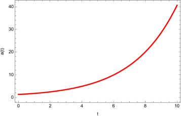
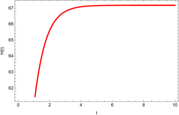
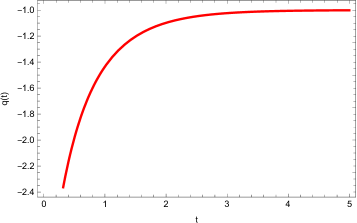
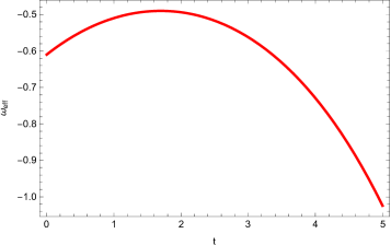
Figure 1: Plots of scale factor, Hubble, deceleration and effective EoS parameters versus cosmic time $t$ for $c_{1}=2$, $c_{2}=1.5$, $c_{3}=-1$, $c_{4}=0.5$, $c_{5}=-1.2$, $c_{9}=3.9$, $c_{13}=-0.99$ and $c_{14}=0.2$.

To study cosmological impact of this exact solution, we establish graphical analysis in Figure 1 (upper left plot) which indicates that positively increasing trajectory corresponds expanding cosmic state. To examine the state of expanding cosmos, we discuss some important cosmological parameters, i.e., Hubble ($H$), deceleration ($q$) and effective equation of state ($w_{eff}$) parameters graphically. The Hubble parameter measures expansion rate of cosmos while deceleration parameter ($q$) specifies the expansion rate as accelerating ($q<0$), decelerating ($q>0$) or constant ($q=0$). The effective EoS parameter categorizes the accelerating and decelerating cosmos into different regimes like radiation ($\omega=\frac{1}{3}$), matter ($\omega=0$), quintessence DE ($-1<\omega\leq-1/3$) and phantom DE ($\omega<-1$) dominated regimes. The mathematical form of these standard parameters is given as

$$H=\frac{\dot{a}}{a},\quad q=-\frac{\dot{H}}{H^{2}}-1,\quad w_{eff}=\frac{p_{{}_{eff}}}{\rho_{{}_{eff}}}=\frac{p_{m}+p_{d}}{\rho_{m}+\rho_{d}}.$$

In the upper right plot of Figure 1, the positively evolving curve measures increasing rate of expansion which is found to be consistent with current value of Hubble parameter, i.e., $H_{0}=67.69\pm 0.68$. Figure 1 (lower left plot) specifies accelerated expansion whereas lower right plot refers to quintessence DE era.

In modified theories of gravity, the minimally coupled $f(R)$ theory of gravity provides the best explanation about enigmatic behavior of cosmos. The framework of $f(R)$ gravity introduces such spectacular models that unfolds mysteries behind early as well as current universe via positive and negative powers of higher derivative of curvature terms [29]. Besides these useful incentives, this ghost-free theory may also illustrate unfeasible behavior due to negative curvature terms. This issue can be eliminated by imposing few constraints on higher-order derivatives, i.e., $f_{R}>0,~{}f_{{}_{RR}}>0$ with $R>R_{0}$, where $R_{0}$ refers to current scalar curvature [30]. In non-minimally coupled $f(R,T)$ theory, Dolgov and Kawasaki suggested an additional constraint such as $1+f(R,T)_{T}>0$. For $f(R,T,Q)$ gravity, the Dolgov-Kawasaki instability analysis leads to the following additional viability conditions

$$\frac{1+f_{{}_{T}}+1/2Rf_{{}_{Q}}}{f_{{}_{R}}-\mathcal{L}_{m}f_{{}_{Q}}}>0,\quad 3f_{{}_{RR}}+(1/2T-T^{00}f_{{}_{RQ}})\geq 0.$$ (46)

The squared speed of sound comes up with simple criteria to discuss stable/unstable nature of new models. For positive squared speed of sound, the linear perturbations become stable due to an oscillatory motion whereas negative squared speed of sound confirms the presence of strong perturbations leading to unstable state. The $r-s$ parameters provide a unique way to explore features of new models as they build a compatibility between constructed and standard cosmological models for their distinct values. For instance, the established model admits a compatibility with $\Lambda$CDM, CDM models and Einstein universe for ($r,s$)=(1,0), (1,0) and (-$\infty$,$\infty$), respectively. If $s>0$ and $r<1$, then model corresponds to quintessence and phantom DE eras while the compatibility with Chaplygin gas model can be observed for $s<0$ and $r>1$. Mathematically, the squared speed of sound and $r-s$ parameters are defined as

$$v_{s}^{2}=\frac{\dot{p_{d}}}{\dot{\rho_{d}}},\quad r=q+2q^{2}-\frac{\dot{q}}{H},\quad s=\frac{r-1}{3(q-\frac{1}{2})}.$$

We establish graphical analysis to study nature of constructed $f(R,Q)$ model (43) via squared speed of sound, viability constraints and $r-s$ parameters. In Figure 2, the upper left plot shows positive evolution of function $f(R,Q)$ whereas positively increasing squared speed of sound identifies stable state of $f(R,Q)$ model in the upper right plot. In the lower panel of Figure 2, the viable nature of non-minimally coupled $f(R,Q)$ model is observed as all conditions are preserved. The left plot of Figure 3 determines compatibility of non-minimally coupled $f(R,Q)$ model with $\Lambda$CDM model as $(r,s)=(1,0)$.

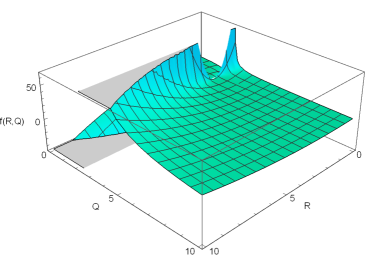
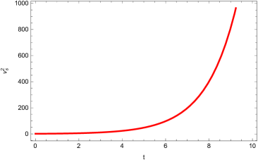
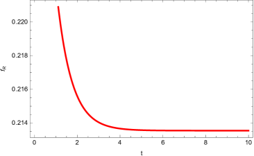
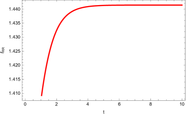
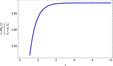
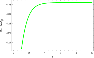
Figure 2: Plots of $f(R,Q)$ (upper left), squared speed of sound (upper right) and viability conditions (lower panel) versus cosmic time $t$.

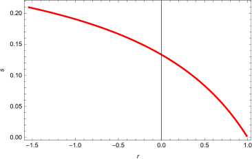
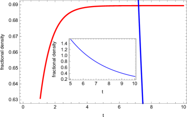
Figure 3: Plots of $r-s$ parameters (left) and fractional densities (right) $\Omega_{m}$ (blue) and $\Omega_{d}$ (red) versus cosmic time $t$.

In the accelerate/decelerated expanding cosmos, the assessment of fractional densities provides observational constraints to counterbalance the contribution of ordinary matter and DE. For flat cosmological model, the fractional densities are restricted to follow $\Omega_{m}+\Omega_{d}=1$ where $\Omega_{m}\simeq 0.3111$ and $\Omega_{d}\simeq 0.6889$ [31]. The mathematical formulation of ordinary matter and DE fractional densities is given by

$$\Omega_{m}=\frac{\rho_{m}}{3m_{pl}^{2}H^{2}},\quad\Omega_{d}=\frac{\rho_{d}}{3m_{pl}^{2}H^{2}}.$$

The right plot of Figure 3 indicates that the fractional densities relative to ordinary matter and DE preserve consistency with Planck 2018 observational data as $\Omega_{d}=0.689$ and $\Omega_{m}=0.303$ for $t=10$.

4 The $f(R,T)$ Model

Here, we discuss the impact of an indirect non-minimal coupling between curvature and matter variables while the generic function $f$ is assumed to be independent of the term $Q$ that induces a direct non-minimal curvature-matter coupling. For this choice of model, we solve the system of equations (18)-(41) with the restriction of non-zero derivatives of $f$ with $Q=0$ and $\mathcal{B}\neq 0$ that yield

$$\chi = Z_{1}(t),\quad\alpha=\frac{-Z_{1}(t)}{8c_{1}\sqrt{a}}+\frac{c_{2}}{\sqrt{a}},\quad\beta=Z_{3}(R),\quad\phi=\frac{-Z_{1}(t)+3c_{2}}{3aZ_{4}(T),_{{}_{T}}},$$

$$\mathcal{B} = Z_{1}(t)+a^{3/2}Z_{1},_{{}_{t}},\quad\psi=0,\quad f(R,T)=c_{1}R+Z_{4}(T),$$

where $c_{1}$ and $c_{2}$ refer to as constants while $Z_{1},~{}Z_{3}$ and $Z_{4}$ denote unknown functions of $t,~{}R$ and $T$, respectively. In order to evaluate the solution of these unknown functions, we use the above values of symmetry generator coefficients and $f(R,T)$ model in Eq.(42) which gives

$$Z_{1}(t) = c_{3}t+c_{4},\quad Z_{3}(R)=c_{9}c_{6},\quad Z_{4}(T)=c_{7}T+c_{8},\quad\rho_{m}(a)=\frac{c_{8}}{c_{7}}-\frac{c_{5}a^{-3}}{c_{7}c_{4}}.$$

Without loss of generality, we redefine $\frac{c_{8}}{c_{7}}=c_{10}$ and $\frac{c_{5}}{c_{4}c_{7}}=c_{11}$. Inserting these solutions into Eq.(16), the respective vector field, boundary term and the $f(R,T)$ model turn out to be

$$Y = (c_{3}t+c_{4})\partial_{{}_{t}}+\left(-\frac{c_{3}t+c_{4}}{8c_{1}\sqrt{a}}+\frac{c_{2}}{\sqrt{a}}\right)\partial_{{}_{a}}+c_{9}c_{6}\partial_{{}_{R}}+\frac{3c_{2}-c_{3}t-c_{4}}{3ac_{7}}\partial_{{}_{T}},$$

$$\mathcal{B} = c_{3}t+c_{4}+c_{3}a^{3/2},\quad f(R,T)=c_{1}R+c_{7}T+c_{8}.$$ (47)

In this case, the $f(R,T)$ model admits an indirect curvature-matter coupling due to linear and independent terms of Ricci scalar and trace of the energy-momentum tensor. The Noether point symmetries and associated first integrals are given by

$$Y_{1} = \frac{1}{\sqrt{a}}\partial_{{}_{a}}+\frac{1}{c_{7}a}\partial_{{}_{T}},\quad I_{1}=6a^{2}\dot{a}f_{{}_{RR}},$$

$$Y_{2} = \partial_{{}_{R}},\quad I_{2}=6\sqrt{a}(2\dot{a}f_{{}_{R}}+a\dot{R}f_{{}_{RR}}+a\dot{T}f_{{}_{RT}})+\frac{6a\dot{a}f_{{}_{RT}}}{c_{7}},$$ (48)

$$Y_{3} = t\partial_{{}_{t}}-\frac{t}{8c_{1}\sqrt{a}}\partial_{{}_{a}}-\frac{t}{3c_{7}a}\partial_{{}_{T}},\quad I_{3}=1-a^{3}(f-Rf_{{}_{R}}-Tf_{{}_{T}}+\rho_{m}(1-f_{{}_{T}}))$$

$$- 6a\dot{a}^{2}f_{{}_{R}}+\frac{12\sqrt{a}\dot{a}f_{{}_{R}}}{8c_{1}}\left(1-8c_{1}\sqrt{a}\dot{a}\right),$$

$$Y_{4} = \partial_{{}_{t}}-\frac{1}{8c_{1}\sqrt{a}}\partial_{{}_{a}}-\frac{1}{3c_{7}a}\partial_{{}_{T}},\quad I_{4}=t+a^{3/2}-ta^{3}(f-Rf_{{}_{R}}-Tf_{{}_{T}}+\rho_{m}$$

$$\times (1-f_{{}_{T}}))+6a\dot{a}^{2}tf_{{}_{R}}-(12a\dot{a}f_{{}_{R}}+6a^{2}\dot{R}f_{{}_{RR}}+6a^{2}\dot{T}f_{{}_{RT}})\left(\dot{a}t+\frac{t}{8c_{1}\sqrt{a}}\right)$$

$$- 6a^{2}\dot{a}\dot{R}f_{{}_{RR}}-6a^{2}\dot{a}tf_{{}_{RT}}(\dot{T}+\frac{1}{3ac_{7}}).$$

In the presence of boundary term, we obtain four symmetry generators and corresponding Noether first integrals. These generators do not appreciate temporal or scaling symmetries and consequently, the respective conservation laws cannot be identified. For the constructed $f(R,T)$ model (47), we solve Eq.(48) to determine exact solution of the scale factor given by

$$a(t)=\frac{1}{4c_{1}^{2}}\left[c_{1}^{2}(I_{2}t+8c_{1}c_{12})\right]^{\frac{2}{3}}.$$

Figure 4 interprets graphical analysis of cosmological parameters for power-law scale factor. The upper left plot shows positively increasing behavior of the scale factor specifying expanding cosmos while the rate of expansion is found to be decreasing as time passes leading to decelerated cosmic expansion (upper right panel). In this case, the deceleration parameter also corresponds to decelerated expanding universe as $q=1/2$. The effective EoS parameter supports this analysis as $0\leq\omega_{eff}<1$ (lower plot). Figure 5 (upper plots) illustrates feasibility of constructed $f(R,T)$ model due to positive squared speed of sound and viability conditions. The $r-s$ parameters fails to achieve compatibility of the established model with any standard cosmological model as $(r,s)=(1,\infty)$. In the lower plot, fractional density of DE dominates over matter density while the dominance of matter energy density is observed as time grows favoring decelerated expansion of the universe.

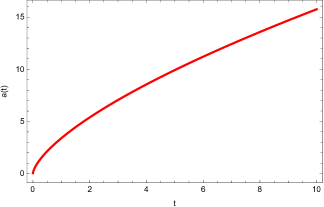
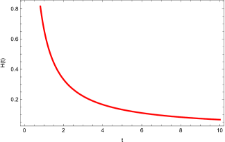
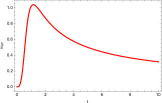
Figure 4: Plots of scale factor, Hubble and effective EoS parameters versus cosmic time $t$ for $c_{1}=c_{8}=c_{11}=0.2$, $I_{2}=10$, $c_{7}=2$, $c_{10}=-1$ and $c_{12}=0.01$.

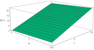
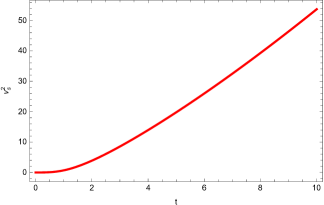
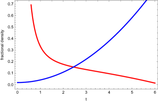
Figure 5: Plots of $f(R,T)$ (left), squared speed of sound (right) and fractional densities $\Omega_{m}$ (blue) and $\Omega_{d}$ (red) versus cosmic time $t$.

5 The $f(T,Q)$ Model

In this section, we consider $T$ and $Q$ to be responsible for strong non-minimal interactions in the absence of Ricci scalar. To study the effect of such interaction on symmetries and conservation laws, we choose $\beta=0$ and restrict generic function to admit non-zero derivatives relative to $T$ and $Q$. The resulting solution of over determining equations (18)-(41) for $\mathcal{B}\neq 0$ is given as

$$\chi=c_{7}t+c_{8},\quad\phi=\frac{T-1/2}{a^{2}c_{4}}\left[a^{2}c_{4}(c_{4}\ln(\frac{2T-1}{2})+c_{3})-\frac{2c_{5}t}{c_{3}}+2c_{4}c_{9}\right],$$

$$\mathcal{B}=c_{5}a+c_{6},\quad\alpha=-\frac{c_{7}a}{3},\quad\psi=c_{10}Q+c_{11},\quad\rho_{m}(a)=\frac{c_{12}\ln a}{2},$$

$$f(T,Q)=c_{1}T+c_{3}Q+c_{4}Q\ln(T-1/2)+c_{2}.$$ (49)

Here $c_{i}^{\prime}s~{}(i=1,2,...,12$) are constants whereas Eq.(49) indicates that the constructed $f(T,Q)$ model induces strong non-minimal interactions. Inserting these solutions into Eq.(16) with $c_{13}=\frac{c_{3}c_{7}}{c_{4}}$, we obtain following set of Noether point symmetries with conserved integrals given by

$$Y_{1} = \partial_{{}_{t}},\quad I_{1}=-a^{3}(f-Tf_{{}_{T}}-Qf_{{}_{Q}}-\rho_{m}(1+f_{T}))+6a\dot{a}^{2}f_{{}_{Q}}(2\rho_{m}+a\rho_{m}^{\prime})$$

$$+ 3a^{2}\dot{a}\rho_{m}(\dot{T}f_{{}_{TQ}}+\dot{Q}f_{{}_{QQ}}),$$

$$Y_{2} = Q\partial_{{}_{Q}},\quad I_{2}=-3a^{2}\dot{a}Q\rho_{m}f_{{}_{QQ}},\quad Y_{3}=\partial_{{}_{Q}},\quad I_{3}=-3a^{2}\dot{a}\rho_{m}f_{{}_{QQ}},$$

$$Y_{4} = -\frac{2t(T-1/2)}{3c_{4}a^{2}}\partial_{{}_{T}},\quad I_{4}=a+\frac{2t(T-1/2)\dot{a}\rho_{m}f_{{}_{TQ}}}{c_{4}}$$

$$Y_{5} = \frac{2c_{9}(T-1/2)}{a^{2}}\partial_{{}_{T}},\quad I_{5}=6(T-1/2)\dot{a}\rho_{m}f_{{}_{TQ}},$$

$$Y_{6} = (T-1/2)\partial_{{}_{T}},\quad I_{6}=-3(T-1/2)a^{2}\dot{a}\rho_{m}f_{{}_{TQ}},$$ (50)

$$Y_{7} = \partial_{{}_{t}}-\frac{a}{3}\partial_{{}_{a}}+(T-1/2)\ln(T-1/2)\partial_{{}_{T}},$$

$$I_{7} = -a^{3}t(f-Tf_{{}_{T}}-Qf_{{}_{Q}}-\rho_{m}(1+f_{T}))+a\dot{a}f_{{}_{Q}}(3\dot{a}t+2a)(2\rho_{m}+a\rho_{m}^{\prime})$$

$$+ a^{3}\rho_{m}(\dot{T}f_{{}_{TQ}}+\dot{Q}f_{{}_{QQ}})-3a^{2}\dot{a}\rho_{m}[(T-1/2)\ln(T-1/2)f_{{}_{TQ}}-t(\dot{T}f_{{}_{TQ}}$$

$$+ \dot{Q}f_{{}_{QQ}})].$$

In the present case, we establish a set of seven symmetry generators together with conserved entities. The Noether point symmetry generator $Y_{1}$ ensures the presence of time translational symmetry identifying energy conservation whereas $Y_{2}$ and $Y_{6}$ define scaling symmetry relative to $Q$ and $T$ yielding conservation of linear momentum. Furthermore, we formulate exact solution for the scale factor by sorting out Eq.(50) that yields

$$a(t)=c_{14}\exp\left[\frac{LambertW\left(-\frac{6I_{6}(t+c_{13}e^{-1})}{c_{12}c_{4}}\right)}{3}+\frac{1}{3}\right]+c_{15}.$$

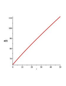
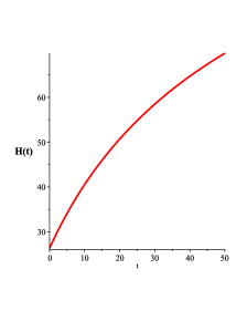
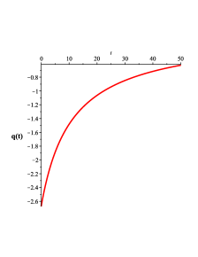
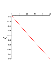
Figure 6: Plots of scale factor, Hubble, deceleration and effective EoS parameters versus cosmic time $t$ for $c_{1}=0.5$, $c_{2}=50$, $c_{3}=0.1$, $c_{4}=-0.18$, $I_{6}=10$, $c_{12}=-1.2$, $c_{13}=10$, $c_{14}=0.1$ and $c_{15}=50$.

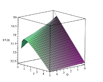
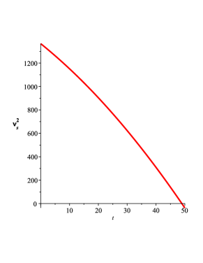
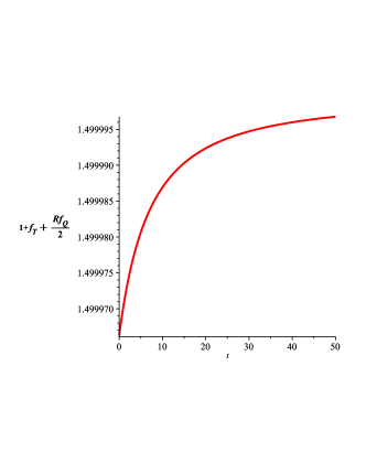
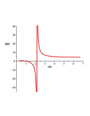
Figure 7: Plots of $f(T,Q)$ (upper left), squared speed of sound (upper right), viability condition (lower left) and $r-s$ parameters (lower right) versus cosmic time $t$.

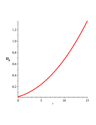
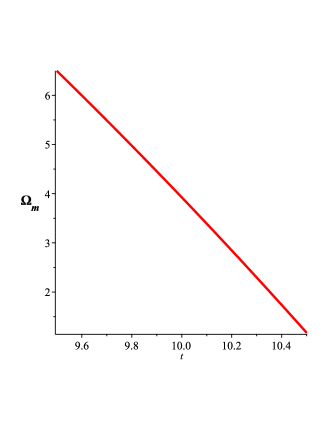
Figure 8: Plots of fractional densities (right) $\Omega_{m}$ (blue) and $\Omega_{d}$ (red) versus cosmic time $t$.

Figure 6 illustrates the evolution of scale factor (upper left plot) while respective cosmological analysis is established via Hubble (upper right), deceleration and effective EoS (lower panel) parameters. The current value of Hubble parameter is achieved as time grows and consequently, the graphical behavior of these parameters supports accelerated quintessence DE era. Figure 7 explores realistic nature of non-minimally coupled $f(T,Q)$ model via squared speed of sound, viability condition and $r-s$ parameters, respectively. In the given range of time, the constructed model is found to be stable and viable whereas initially, it preserves consistency with $\Lambda$CDM model. In Figure 8, the fractional density of DE is compatible with Planck’s constraints at $t=10$ whereas matter energy density exceeds from the suggested value at the same time. Thus, the total fractional energy density fails to achieve $\Omega_{m}+\Omega_{d}=1$.

6 The $f(R,T,Q)$ Model

In the present case, we determine Noether point symmetries with conserved entities and also study the behavior of generic function $f$ in the presence of non-minimally interacting scalar curvature and matter variables. For non-zero boundary term, we consider $\beta=0$, $\chi=\mathcal{B}=\alpha=\varphi(t,a)$ and restrict generic function to have non-zero first order derivatives relative to independent variables $R,~{}T$ and $Q$. Inserting these constraints into Eqs.(18)-(37), we obtain

$$\chi=F_{1}(t),\quad\mathcal{B}=F_{2}(t),\quad\alpha=F_{3}(a),\quad\phi=F_{4}(a,R,T,Q),$$

$$f(R,T,Q)=F_{5}(T)R+QF_{6}(T)+F_{(}7).$$

Here $F_{i}^{\prime}s,~{}(i=1,2,...,7)$ are unknown functions. For above solutions, we solve Eqs.(38)-(42) which yield

$$F_{1}(t)=c_{2},\quad F_{3}(a)=\frac{c_{1}}{\sqrt{a}},\quad F_{5}(T)=c_{3},\quad\rho_{m}=\frac{c_{4}}{a^{\frac{3}{2}}},$$

$$\psi=-[3c_{1}a^{\frac{3}{2}}(QTF_{{}_{6T}}+TF_{{}_{7T}}-F_{{}_{7}})+a^{3}QTF_{4}F_{{}_{6TT}}+a^{3}QF_{4}F_{{}_{6T}}+a^{3}TF_{4}$$

$$F_{{}_{7TT}}+F_{{}_{2t}}]/[a^{3}TF_{{}_{6T}}].$$

Verifying the resulting solution for $F_{6}=F_{7}$, we get

$$F_{2}(t)=c_{5}t,\quad F_{6}(T)=c_{6}T+c_{7},\quad F_{4}(a,R,T,Q)=\frac{9Tc_{8}+4c_{9}a}{4a\sqrt{a}}.$$

The explicit from of $f(R,T,Q)$ model turns out to be

$$f(R,T,Q)=c_{3}R+(Q+1)(c_{6}T+c_{7}).$$ (51)

It is worth noting that the constructed model induces strong non-minimal interactions between $T$ and $Q$ whereas the Noether symmetries with boundary and associated conserved integral are given by

$$Y_{1} = \partial_{{}_{t}},\quad I_{1}=-a^{3}(f-Rf_{R}-Tf_{{}_{T}}-Qf_{{}_{Q}}-\rho_{m}(1+f_{T}))$$

$$- 6a\dot{a}^{2}f_{{}_{R}}-3a^{2}\dot{a}\rho_{m}\dot{T}f_{{}_{TQ}}+9a^{2}\dot{a}^{2}\rho_{m}^{\prime}f_{{}_{Q}}),$$

$$Y_{2} = \frac{1}{\sqrt{a}}\partial_{{}_{a}}-\frac{3Q}{4a\sqrt{a}}\partial_{{}_{Q}},$$

$$I_{2} = 12\sqrt{a}\dot{a}f_{{}_{R}}-6\sqrt{a}\dot{a}f_{{}_{Q}}(2\rho_{m}+a\rho_{m}^{\prime})+3a\sqrt{a}\dot{T}\rho_{m}f_{{}_{TQ}},$$

$$Y_{3} = \frac{9}{16a\sqrt{a}}\left(4T\partial_{{}_{T}}-Q\partial_{{}_{Q}}\right),\quad I_{3}=-\frac{27a^{2}\dot{a}\rho_{m}f_{{}_{TQ}}T}{4a\sqrt{a}},$$ (52)

$$Y_{4} = \frac{1}{T\sqrt{a}}\left(T\partial_{{}_{T}}-Q\partial_{{}_{Q}}\right),\quad I_{4}=-\frac{3a^{2}\dot{a}\rho_{m}f_{{}_{TQ}}}{\sqrt{a}}.$$

Here, we formulate four symmetries together with Noether first integrals while there is only one symmetry generator that corresponds to time translational symmetry and respective Noether integral specifies energy conservation. For constructed $f(R,T,Q)$ model (51), the conserved integral $I_{3}$ yields

$$a(t)=\frac{(-9c_{4}^{2}c_{6}(-9c_{10}c_{4}^{2}c_{6}+2I_{3}t)^{2})^{\frac{2}{3}}}{(-9c_{10}c_{4}^{2}c_{6}+2I_{3}t)^{2}}.$$

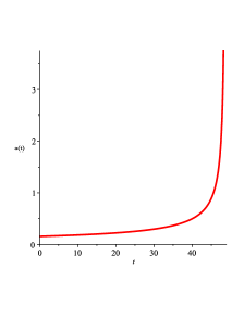
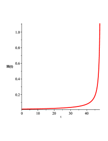
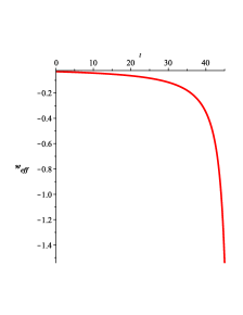
Figure 9: Plots of scale factor, Hubble and effective EoS parameters versus cosmic time $t$ for $c_{3}=15$, $c_{4}=0.5$, $c_{6}=-13.5$, $c_{7}=1.5$, $I_{3}=5$ and $c_{10}=-16$.

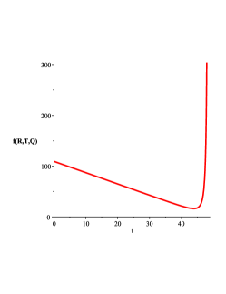
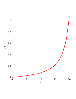
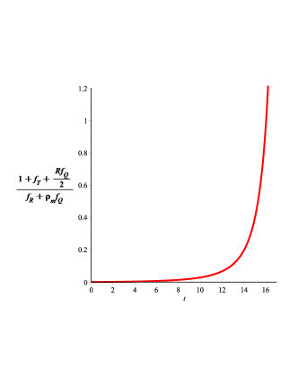
Figure 10: Plots of $f(R,T,Q)$ (upper left), squared speed of sound (upper right) and viability condition (lower plot) versus cosmic time $t$.

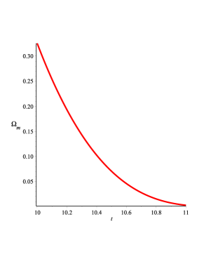
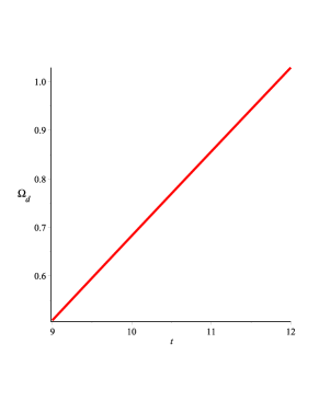
Figure 11: Plots of fractional densities $\Omega_{m}$ (left) and $\Omega_{d}$ (right) versus cosmic time $t$.

In Figure 9, we discuss cosmological impact of the above exact solution through standard parameters which indicates that the universe meets up with accelerated expansion. Furthermore, the negative value of deceleration parameter ($q=-2.5$) ensures accelerated expansion of the universe. The graphical analysis of effective EoS parameter illustrates that the cosmos enters into quintessence DE era and gradually joins phantom DE phase (lower plot). For numerical value of deceleration parameter, the $(r,s)=(3.75,0.38)$ parameters characterize Chaplygin gas model. Figure 10 identifies stable as well viable behavior of positively evolving non-minimally coupled $f(R,T,Q)$ model in the background of DE. In Figure 11, the fractional energy densities follow observational constraints in the given time interval.

7 Final Remarks

The revolutionary idea of non-minimal coupling between geometry and matter sectors leads to fascinating approaches that explore different cosmological scenarios as well as cosmic evolution from its origin to the current state. The present work is devoted to study evolutionary stages of flat and isotropic cosmos filled with dust distribution in the background of $f(R,T,Q)$ gravity. For this purpose, we have followed Noether Gauge symmetry technique that induces temporal or spatial symmetries along with relevant conservation laws, i.e., energy or linear/angular momentum conservation, respectively. Besides symmetries and respective conservation laws, this intriguing technique also helps to formulate exact solution to understand corresponding cosmological impact.

The presence of strong or weak non-minimal interactions between curvature and matter variables investigate different cosmological phenomenologies. In the this work, we have considered different choices for generic function $f(R,T,Q)$ admitting non-minimal interactions such as $f(R,Q)$, $f(R,T)$ and $f(T,Q)$ models independent of $T,~{}Q$ and $R$, respectively. For each choice and general $f(R,T,Q)$ model, we have found explicit forms of generic function as well as discussed the existence of Noether point symmetries together with conservation laws in the presence of boundary term. The summary for formulated symmetries and respective conservation laws for $\mathcal{B}\neq 0$ is given in Table 1.
Table 1: Symmetries and Conservation laws for $\mathcal{B}\neq 0$.

Model	Symmetry	Conservation Laws
$f(R,Q)$	Temporal $\&$ scaling	Energy $\&$ Linear Momentum
$f(T,Q)$	Temporal $\&$ scaling	Energy $\&$ Linear Momentum
$f(R,T,Q)$	Temporal	Energy conservation

It is interesting to mention here that for $f(R,T)$ model with $\mathcal{B}\neq 0$, the system of over determining equations fail to produce any well-known symmetry and conservation law. In each case, the conserved integrals yield exact solutions for scale factor. We have investigated cosmological features of these solutions via graphical analysis of some standard cosmological parameters, i.e., Hubble, deceleration and effective EoS parameters. Planck 2018 suggested different values of $H$ at $68\%CL$ given by [31]

$$H_{0} = 67.27\pm 0.60\quad\text{(TT+TE+EE+low E)},$$

$$H_{0} = 67.36\pm 0.54\quad\text{(TT+TE+EE+low E+lensing)},$$

$$H_{0} = 67.66\pm 0.42\quad\text{(TT+TE+EE+low E+lensing+BAO)}.$$

Furthermore, we have examined stable/unstable and viable/unviable state of constructed $f(R,Q),~{}f(R,T),~{}f(T,Q)$ and $f(R,T,Q)$ models through squared speed of sound and viability conditions suggested by Dolgov-Kawasaki instability analysis. The contribution of matter content is also studied by analyzing fractional densities of dust fluid and DE. The observational values of $\Omega_{m}$ and $\Omega_{d}$ with $68\%$ percent limit are given as [31]

$$\Omega_{m} = 0.3166\pm 0.0084\quad\text{(TT+TE+EE+low E)},$$

$$\Omega_{m} = 0.3158\pm 0.0073\quad\text{(TT+TE+EE+low E+lensing)},$$

$$\Omega_{m} = 0.3111\pm 0.0056\quad\text{(TT+TE+EE+low E+lensing+BAO)}$$

$$\Omega_{d} = 0.7116\pm 0.0084\quad\text{(TT+TE+EE+low E)},$$

$$\Omega_{d} = 0.6847\pm 0.0073\quad\text{(TT+TE+EE+low E+lensing)},$$

$$\Omega_{d} = 0.68889\pm 0.0056\quad\text{(TT+TE+EE+low E+lensing+BAO)}$$

The consistency of all parameters is checked against Planck’s 2018 observational data. The results are summarized as follows.

• $f(R,Q)$ Model

In the presence of boundary term, the graphical analysis of cosmological parameters supports accelerated cosmic expansion as current value of Hubble parameter is achieved, deceleration parameter is negative while effective EoS parameter corresponds to quintessence DE phase. The constructed non-minimally coupled $f(R,Q)$ model is found to be stable, viable and compatible with $\Lambda$CDM model. The fractional densities are consistent with Planck suggested constraints. Zubair et al. [32] investigated cosmic evolution using particular $f(R,Q)$ model and power-law Hubble parameter without using Noether Symmetry approach. They constructed model constraints that referred to $\Lambda$CDM limit and explains current accelerated expansion.

• $f(R,T)$ Model

The cosmological parameters are found to be in favor of decelerated expanding cosmos due to decreasing rate of expansion, positive deceleration parameter and correspondence of effective EoS parameter with radiation dominate era. The stable as as well as viable $f(R,T)$ model admits minimal coupling between scalar curvature and matter though it does not appreciate compatibility with any standard cosmological model. In the background of radiation-dominated phase, the fractional density relative to dust fluid dominates over DE fractional density ensuring decelerated expanding cosmos. We have discussed the presence of Noether Gauge symmetry in $f(R,T)$ theory [33]. For this purpose, we considered minimally coupled $f(R,T)$ model that admits symmetry generator relative to energy conservation whereas exact solution for the scale factor is not measured. In the present work, we have found $f(R,T)$ model appreciating minimal interactions between curvature and matter variables while power-law exact solution is obtained that defines decelerated expanding cosmos.

• $f(T,Q)$ Model

The graphical study of cosmological parameters leads to accelerated expansion of the universe for Noether Gauge symmetries. We have formulated non-minimally coupled $f(T,Q)$ model that preserves stability and viability conditions while consistency with $\Lambda$CDM model is achieved for $\mathcal{B}\neq 0$. The fractional densities are inconsistent with accelerated expanding cosmos for non-zero boundary term.

• $f(R,T,Q)$ Model

In this case, the graphical interpretation demonstrates accelerated expansion with a transition from quintessence to phantom regions. The established $f(R,T,Q)$ model incorporates non-minimal coupling between $T$ and $Q$ while appreciates minimal coupling with $R$. The model is found to be feasible as $v_{s}^{2}>0$ and viability condition are satisfied. This realistic model admits compatibility with Chaplygin gas model whereas graphical illustration of fractional densities also correspond to accelerated expanding cosmos.

We have found symmetry generators and conserved quantities for each case except for $f(R,T)$ model, where symmetries and respective conservation laws do not correspond to any standard symmetry or conserved entity. The constructed $f(R,T,Q)$ models are found to be stable and viable. The compatibility of established models with $\Lambda$CDM and Chaplygin gas models is observed. We conclude that the constructed solutions favor accelerated cosmic expansion whenever generic function involves non-minimal coupling with $Q$.

Data Availability Statement: No new data were created or analyzed in this study.

References

[1] Sotiriou, T.P. and Faraoni, V.: Rev. Mod. Phys.
82(2010)451; Felice, A.D. and Tsujikawa, S.: Living Rev.
Rel. 13(2010)3; Nojiri, S. and Odintsov, S.D.: Phys. Rept.
505(2011)59.
[2] Bertolami, O. et al.: Phys. Rev. D 75(2007)104016.
[3] Harko, T. et al.: Phys. Rev. D 84(2011)024020.
[4] Bertolami, O. and Sequeira, M.C.: Phys.
Rev. D 79(2009)104010; Bertolami, O., Frazo, P.
and Pramos, J.: Phys. Rev. D 81(2010)104046;
ibid. 83(2011)044010.
[5] Sharif, M. and Zubair, M.: J. Cosmol. Astropart. Phys.
03(2012)028; J. Phys. Soc. Jpn. 82(2013)014002;
ibid. 82(2013)064001; Gen. Relativ. Gravit.
46(2014)1723.
[6] Odintsov, S.D. and Saez-Gomez, D.: Phys. Lett. B
725(2013)437.
[7] Harko,T. and Lobo, F.S.N.: Int. J. Mod. Phys. D
29(2020)2030008.
[8] Haghani, Z. et al.: Phys. Rev. D 88(2013)044023.
[9] Sharif, M. and Zubair, M.: J. Cosmol. Astropart. Phys.
11(2013)042; J. High Energy Phys. 12(2013)079.
[10] Yousaf, Z. et al.: Eur. Phys. J. A 54(2018)122;
Bhatti, M.Z. et al.: J. Cosmol. Astropart. Phys.
09(2019)011.
[11] Sebastiani, L. and Zerbini, S.: Eur. Phys. J. C
71(2011)1591.
[12] Maharaj, S.D. et al.: Mod. Phys. Lett. A 32(2017)1750164.
[13] Sharif, M. and Zubair, M.: Astrophys. Space Sci.
349(2014)457.
[14] Harko, T. and Lake, M.J.: Eur. Phys. J. C 75(2015)60.
[15] Shamir, M.F. and Raza, Z.: Astrophys. Space Sci. 356(2015)111.
[16] Shamir, M.F.: Eur. Phys. J. C 75(2015)354.
[17] Capozziello, S., Stabile, A. and Troisi, A.: Class. Quantum Grav.
24(2007)2153.
[18] Hussain, I., Jamil, M. and Mahomed, F.M.: Astrophys. Space Sci.
337(2012)373.
[19] Shamir, M.F., Jhangeer, A. and Bhatti, A.A.: Chin. Phys. Lett.
29(2012)080402.
[20] Atazadeh, K. and Darabi, F.: Eur. Phys. J. C 72(2012)2016.
[21] Momeni, D., Myrzakulov, R. and Gdekli, E.: Int. J. Geom.
Methods Mod. Phys. 12(2015)1550101.
[22] Sharif, M. and Fatima, I.: J. Exp. Theor. Phys. 122(2016)104.
[23] Sharif, M. and Nawazish, I.: J. Exp. Theor. Phys. 120(2014)49;
Eur. Phys. J. C 77(2017)198; Mod. Phys. Lett. A
32(2017)1750136.
[24] Sharif, M. and Nawazish, I.: Ann. Phys. 389(2018)283;
ibid. 400(2019)37.
[25] Sharif, M., Nawazish, I. and Hussain, S.: Eur. Phys.
J. C 80(2020)783
[26] Bertolami, O., Pedro, F.G. and Le Delliou, M.: Phys.
Lett. B 654(2007)165; Damour, T.: Compt. Rend. Acad. Sci.
Ser. IV Phys. Astrophys. 2(2001)1249.
[27] Sotiriou, T.P. and Faraoni, V.: Class.
Quantum Grav. 25(2008)205002; Bertolami, O. and
Pramo, J.: Class. Quantum Grav. 25(2008)245017.
[28] Basilakos, S., Tsamparlis, M. and Paliathanasis, A.: Phys. Rev. D
83(2011)103512; ibid. 84(2011)123514; Basilakos,
S. et al.: Phys. Rev. D 88(2013)103526; Paliathanasis, A.
et al.: Phys. Rev. D 89(2014)063532.
[29] Capozziello, S.: Int. J. Mod. Phys. D 11(2002)483;
Nojiri, S. and Odintsov, S.D.: Gen. Relativ. Gravit.
36(2004)1765.
[30] Dolgov, A.D. and Kawasaki, M.: Phys. Lett. B 573(2003)1;
Faraoni, V.: Phys. Rev. D 74(2006)104017.
[31] Aghanim, N. et al.: Astron. Astrophys. A6(2020)641.
[32] Zubair, M., Zeeshan, M. and Waheed, S.: Mod. Phys. Lett. A 34(2019)1950253.
[33] Sharif, M. and Nawazish, I.: Gen. Relativ. Gravit. 49(2017)76.