Mixing effects on spectroscopy and partonic observables of mesons with logarithmic confining potential in a light-front quark model

Abstract

Using the variational principle, we systematically investigate the mass spectra and wave functions of both $1S$ and $2S$ state heavy pseudoscalar $(P)$ and vector $(V)$ mesons within the light-front quark model. This approach incorporates a Coulomb plus logarithmic confinement potential to accurately describe the constituent quark and antiquark dynamics. Additionally, spin hyperfine interactions are introduced perturbatively to compute the masses of pseudoscalar and vector mesons. The present analyses of the $1S$ and $2S$ states require the consideration of mixing between them to account for empirical constraints. These constraints include the mass gap $\Delta M_{P}>\Delta M_{V}$, where $\Delta M_{P(V)}=M^{2S}_{P(V)}-M^{1S}_{P(V)}$ and the hierarchy of the decay constants $f_{1S}>f_{2S}$. We find the optimal value of the mixing angle to be $\theta=18^{\circ}$, significantly enhancing the consistency between our spectroscopic predictions and the experimental data compiled by the Particle Data Group (PDG). Furthermore, based on the predicted mass, the newly observed resonance $B_{J}(5840)$ could be assigned as a $2^{1}S_{0}$ state in the $B$ meson family. The study also reports various pertinent observables, including twist-2 distribution amplitudes, electromagnetic form factors, charge radii, $\xi$ moments, and transition form factors which are found to be consistent with both available lattice simulations and experimental data. In addition, our predicted branching ratios for the channels of $B^{+}\rightarrow\tau^{+}\nu_{\tau}$ as well as rare decays of $B^{0}$ and $B_{s}^{0}$ appear in accordance with experimental data.

I Introduction

Typical descriptions of various meson properties are encapsulated by either Euclidean or Minkowski approach. Calculations and simulations in the Euclidean approach typically involve Euclidean time for the analyses of two- and three-point correlation functions, with source and sink operators specifying hadron states. The Euclidean approach Shifman19791 ; bali2018 ; asgarian2021 ; Dudek2006 ; padmanath2015 ; cooper2022 is employed not only in the Lattice Gauge Theories with large time separation but also in the QCD Sum Rule (QCDSR) calculations with operator product expansions. It provided a wealth of valuable insights into the behavior of quarks and gluons within hadrons. In the Minkowski approach, various model-building frameworks were developed to explore useful insights into the characteristics of hadrons. The static properties, such as mass spectroscopy, were estimated by traditional quark models employing specific Hamiltonians that primarily incorporate the Coulomb force at short distances and the confinement force at large distances, characterized by various potential terms. Such models have achieved remarkable success, notably in providing detailed descriptions of mesons rosner2008 ; Ebert:2009ua ; shah20141 ; Godfrey2016 ; pandya2021 . For the relativistic Hamiltonians, the light-front (LF) quantization has been utilized to incorporate factorization theorems of perturbative QCD alongside non-perturbative correlation functions such as parton distribution functions (PDFs) and distribution amplitudes (DAs) to examine hard inclusive and exclusive processes, respectively, in terms of the non-perturbative LF wave functions (LFWFs) of hadrons choi2009 ; ke2010 ; chang2018 ; hwang2012 ; Dhiman2019 ; adhikari2021 ; lan2019 . The newer development with the holographic QCD describing hadrons as quantum fields propagating into bulk fields with extra dimensions has also been efficient in predicting mass spectroscopy karch2006 ; paula2009 ; de2009 ; branz2010 ; swarnkar2015 ; chang2017 ; Gurjar:2024wpq ; Ahmady:2022dfv ; Ahmady:2021yzh ; Li:2022izo ; Li:2021jqb ; deTeramond:2021yyi . The holographic platform implemented the confinement through the dilatation with the choice of soft vs. hard walls, incorporating quark-related fields via the infinite limit of $N_{c}$ and $N_{f}$.

In the present work, we utilize the light-front quark model (LFQM) based on the light-front dynamics (LFD) in the Minkowski approach to analyze both the meson spectroscopy and structures simultaneously. Within the LFQM formalism, the hadronic wave function comprises equal LF time quantization naturally incorporating relativistic effects. Due to the rational energy-momentum dispersion relation in LFD, there is a sign correlation between the LF energy and LF longitudinal momentum. This feature provides the distinguished characteristic of the vacuum property in the LFD, sweeping the non-trivial vacuum condensation effects into the LF zero modes (LFZMs), i.e. the modes with zero LF longitudinal momentum, and leaving the rest of the vacuum clean by suppressing the quantum fluctuations of the non-LFZMs in the vacuum. Moreover, the longitudinal and transverse boost operators in LFD are kinematical and thus the LFWFs are completely boost invariant, i.e. independent of reference frames brodsky1998 ; Choi1999 . Namely, the meson LFWFs obtained in the meson rest frame are identical to the corresponding LFWFs obtained in any other moving frames. These remarkable features make the LFQM a promising theory for the phenomenological study of hadron properties. Due to the simultaneous analyses of both spectroscopy and structures, one can analyze various physical observables and correlation functions including mass spectra, decay constants, form factors, DAs, PDFs, generalized parton distributions (GPDs), etc., all within a single designated LFQM.

Early endeavors in the study of LFQM involved the successful utilization of the standard Cornell potential, where confinement exhibits linear behaviour Choi2015 . Subsequent efforts have investigated alternative approaches, including harmonic and exponential confinements Dhiman2019 . Given that previous studies on LFQM exclusively addressed ground states, the structure and features of radially excited states have not received much attention in these models. However, in a recent study  Arifi2022 , two of us computed ground and radial excited states using a Coloumb plus linear confinement potential in variational calculations, utilizing the two lowest-order harmonic oscillator basis functions. The study reports mass spectra for the 1S and 2S states both without and with consideration of mixing effects in the wave function.

The analysis of the first radial excited state is significant in assessing two important empirical hierarchies observed from the experimental data. These include the higher mass gap between pseudoscalar states compared to vector states, denoted as $\Delta M_{P}>\Delta M_{V}$, where $\Delta M_{P(V)}=M^{2S}_{P(V)}-M^{1S}_{P(V)}$. Additionally, it involves the larger decay constant of the ground state in comparison to the radial excited states, given as $f_{1S}>f_{2S}$. From this study, it is apparent that there is not much disparity between the masses predicted by the pure and mixed treatment of wave functions Arifi2022 . However, mixing effects are necessary for explaining the aforementioned hierarchies. With the inclusion of mixing effects, the prediction made in Ref. Arifi2022 has a $\chi^{2}$ analysis value of 0.009 with respect to the experimental data. Also, the predictions from the exponential confinement show a disparity compared to the experimental results, with a $\chi^{2}$ analysis value of 0.012 for ground state heavy-light mesons.

Except for the exponential confinement, all prior attempts have used potentials that belong to a special choice of the well-known general potential, $-Cr^{-\alpha}+Dr^{\beta}+V_{0}$ with $V_{0}=a$, $\alpha=1$ and $\beta=\nu$  Lucha1991 ; Patel2009 . However, the pure phenomenological potential, such as the logarithmic potential $V(r)=c\ln(r/r_{0})$ suggested by Quigg and Rosner Quigg1977 ; Rosner1979 , is believed to be successful in heavy-light and heavy-heavy meson spectroscopy. As far as the structural properties of mesons are concerned, the logarithmic potential indicates $n~{}|\psi(0)|^{2}$ is constant, where $n$ is the principle quantum number and $|\psi(0)|^{2}$ is the square of wave function at the origin. This is in contrast to other potentials with power-law forms $V\sim r^{\epsilon}$ where $\epsilon>0$, $|\psi(0)|^{2}\sim n^{2(\epsilon-1)/(2+\epsilon)}$ Quigg1977 ; Rosner1979 . In this respect, the logarithmic potential exhibits a unique characteristic of producing level spacings independent of quark mass and flavour  Quigg1977 ; Rosner1979 . This property contributes to the attractiveness of the logarithmic potential model in describing certain aspects of meson spectroscopy. Since the potential energy between the quark and antiquark varies logarithmically with their separation distance, the resulting energy spectrum tends to have more uniform level spacings, regardless of the quark masses or other characteristics. This feature is particularly intriguing, as the experimental data show that the mass gap between the $1S$ and $2S$ states is around 600 MeV, almost independent of the heavy flavors, exhibiting some degree of universality. This motivates us to comparatively analyze heavy flavor mesons using both the logarithmic potential and the typical linear potential, including both $1S$ and $2S$ states.

Hence, we aim to study the mass spectra and other related properties closely following the scheme developed in Choi:2007yu but with the use of a logarithmic potential for mesons. Additionally, we seek to assess the impact of mixing effects on the observed experimental hierarchies. The $B$ meson spectrum has been enriched by the observation of novel states $B_{J}(5840)$ and $B_{J}(5960)$ by the LHC_b Collaboration LHCb2015 . Additionally, the new resonance labelled as $D_{s}(2590)$ was recorded by LHC_b very recently Lhcb2021ds . Their experimental properties and mass range make them suitable candidate for the first radially excited state. However, their true identification is pending, and where to place them in the existing mass spectrum of $B$ and $D_{s}$ mesons remains an open problem. The present study of radially excited states could also aid in their identification. Along with the mass spectra, pseudoscalar decay constants cover a wide range of applicability including the di-leptonic decays of ground state pseudoscalar mesons in heavy-light sector. Estimation of these flavour changing neutral current transitions opens a window to possible existence of new physics. The connection between di-leptonic decays and partonic observables in heavy-light mesons lies in their shared goal of probing the fundamental interactions and structure of hadrons as the the momentum distribution amplitude for the constituent quark and antiquark inside the mesons are being measured immediately before their annihilation to lepton pairs. Thus, we also address well-known weak decays of heavy-light mesons as a complementary information from present study.

The remainder of the paper is structured as follows. In subsequent Sec. II, we outline the formalism which includes the inter quark-antiquark potential, effective Hamiltonian and trial wave functions employed in the present study. We also discuss the procedure of determining our model parameters following the variational principle within LFQM. In Sec. III, we summarize the explicit formulas to obtain the various physical quantities such as decay constants, DAs and electromagnetic form factors (EMFFs), transition form factors (TFFs) of quarkonia and di-leptonic decays of heavy-light mesons within LFQM. Our numerical results are presented and discussed in Sec. IV followed by the summary in Sec. V.

II Model Description

The stationary meson system is characterized as an interacting bound-state consisting of valence quark and antiquark that are effectively dressed. This system conforms to the eigenvalue equation derived from the effective Hamiltonian motivated by QCD given by

$$H_{q\bar{q}}|\Psi_{q\bar{q}}\rangle=M_{q\bar{q}}|\Psi_{q\bar{q}}\rangle,$$ (1)

where $M_{q\bar{q}}$ and $\Psi_{q\bar{q}}$ are the mass eigenvalue and eigenfunction of the $q{\bar{q}}$ meson bound state, respectively. The effective Hamiltonian in the $q{\bar{q}}$ center of mass frame is represented as

$$H_{q\bar{q}}=H_{0}+V_{q\bar{q}}{,}$$ (2)

where $H_{0}$ is the relativistic kinetic energy term given by

$$H_{0}={\sqrt{m_{q}^{2}+{\mathbf{k}}^{2}}}+{\sqrt{{m_{\bar{q}}^{2}+{\mathbf{k}}^{2}}}}$$ (3)

Here, $m_{q(\bar{q})}$ is the mass of the constituent quark (antiquark) with three momentum $\textbf{k}=({\bf k}_{\perp},k_{z})$. The usual quark-antiquark interaction potential $V_{q\bar{q}}$ is typically modeled as the sum of a short-distance Coulomb part $V_{\text{Coul}}$ and a long-distance confining part $V_{\text{Conf}}$. Upon inclusion of the spin-dependent hyperfine interaction $V_{\text{Hyp}}$, $V_{q\bar{q}}$ takes the following form

$$V_{q\bar{q}}=V_{\text{Coul}}\,+V_{\text{Conf}}\,+V_{\text{Hyp}}{.}$$ (4)

The Coulomb potential is given by

$$V_{\text{Coul}}=-\frac{4\alpha_{s}}{3r},$$ (5)

where $\alpha_{s}$ is the strong coupling constant and considered in present scheme as a free parameter, whereas $r$ is the distance between quark and antiquark. For the confining potential, we take the logarithmic potential given by Quigg1977 ; Rosner1979

$$V_{\text{Conf}}=\,a+\,c\,\ln{(r/{r_{0}})},$$ (6)

where $c$ and $r_{0}$ are the logarithmic confinement parameters adopted from Quigg1977 ; Rosner1979 . Similarly, the hyperfine interaction potential, which is related to effective one-gluon exchanges and describes the spin-dependent part of the interaction between quarks within hadrons, is given by

$$V_{\text{Hyp}}={\frac{32\pi\alpha_{s}}{9}}\frac{\left(\textbf{S}_{q}\cdot\textbf{S}_{\bar{q}}\right){\delta^{3}\left(\textbf{r}\right)}}{m_{q}m_{\bar{q}}}{,}$$ (7)

where $\langle\textbf{S}_{q}\cdot\textbf{S}_{\bar{q}}\rangle$ represents the spin-spin interaction contribution, having values of ${1/4}$ for spin triplet states and ${-3/4}$ for spin singlet states, respectively. We note that the two potential parameters $a$ and $\alpha_{s}$ are to be determined later.

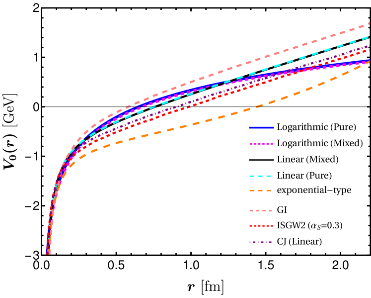
Figure 1: Variation of central potential as a function of inter quark distance $\mathbf{r}$ (in fm) for pure and mixed scenarios. The potential behaviour from other studies Linear Arifi2022 , Exponential Dhiman2019 , GI Godfrey1985 , ISGW2 Scora1995 and old CJ Choi20071 are also presented for comparison.

For the four-momentum $P^{\mu}=\left(P^{+},P^{-},\textbf{P}_{\bot}\right)$ of a meson and the four-momentum $p^{\mu}_{i}$ of the $i$th constituent quark $(i=1,2)$, the LFWF of the meson is represented by Lorentz invariant internal variables and helicity $\lambda_{i}$. The internal variables include the longitudinal momentum fraction $x_{i}=p_{i}^{+}/P^{+}$ and the relative transverse momentum $\textbf{k}_{{\bot}i}=\textbf{p}_{{\bot}i}-{x_{i}}\textbf{P}_{{\bot}}$ of the $i$th quark, which satisfy $\sum_{i=1}^{2}\,x_{i}\,=\,1$ and $\sum_{i=1}^{2}\textbf{k}_{\perp i}\,=\,0$. We assign $i=1$ to the quark and $i=2$ to the antiquark, and define $x\equiv x_{1}$ and ${\bf k}_{\perp}\equiv{\bf k}_{\perp 1}$. Then, the three-momentum ${\bf k}=(k_{z},{\bf k}_{\perp})$ can be written in terms of $(x,{\textbf{k}_{\perp}})$ as $k_{\textit{z}}=\left(x-\frac{1}{2}\right)M_{0}+\frac{{m_{\bar{q}}^{2}}-{m_{q}^{2}}}{2M_{0}}{,}$ where

$$M_{0}^{2}=\frac{\textbf{k}_{\bot}^{2}+m_{q}^{2}}{x}+\frac{\textbf{k}_{\bot}^{2}+m_{\bar{q}}^{2}}{1-x}$$ (8)

is the boost-invariant meson mass squared. The Jacobian factor for the variable transformation $\{k_{z},{\bf k}_{\perp}\}\to\{x,{\textbf{k}_{\perp}}\}$ is given by $\frac{\partial k_{\textit{z}}}{\partial x}=\frac{M_{0}}{4x(1-x)}\Big{[}1-\frac{(m_{q}^{2}-m_{\bar{q}}^{2})^{2}}{M_{0}^{4}}\Big{]}.$

The LFWF $\Psi_{q\bar{q}}=\Psi_{nS}^{J,J_{z}}$ for the $n$S state meson in momentum space is then given by Choi:2007yu

$${\Psi}_{nS}^{JJ_{z}}\left(x,\textbf{k}_{\bot},\lambda_{i}\right)=\Phi_{nS}\left(x,\textbf{k}_{\bot}\right)\mathcal{R}_{{\lambda_{q}}{\lambda_{\bar{q}}}}^{JJ_{z}}\left(x,\textbf{k}_{\bot}\right){,}$$ (9)

where $\Phi_{nS}\left(x,\textbf{k}_{\bot}\right)$ and $\mathcal{R}_{{\lambda_{q}}{\lambda_{\bar{q}}}}^{JJ_{z}}\left(x,\textbf{k}_{\bot}\right)$ are the radial and spin-orbit wave functions, respectively. The spin-orbit wave function can be derived from the ordinary equal-time static one with assigned quantum number $J^{PC}$ through the interaction-independent Melosh transformation. Essentially, it is more convenient to use the covariant form of $\mathcal{R}_{{\lambda_{q}}{\lambda_{\bar{q}}}}^{J{J_{z}}}$ for pseudoscalar and vector mesons as Jaus1990

$$\mathcal{R}_{{\lambda_{q}}{\lambda_{\bar{q}}}}^{00}=\frac{-1}{\sqrt{2}{\widetilde{M}_{0}}}\ \bar{{u}}_{\lambda_{q}}(p_{q})\ \gamma_{5}\ {v}_{\lambda_{\bar{q}}}(p_{\bar{q}}){,}$$ (10)

$$\mathcal{R}_{{\lambda_{q}}{\lambda_{\bar{q}}}}^{1J_{z}}=\frac{-1}{\sqrt{2}{\widetilde{M}_{0}}}\,{\bar{u}}_{\lambda_{q}}(p_{q})\Big{[}\not{\epsilon}(J_{z})-\frac{\epsilon\cdot(p_{q}-p_{\bar{q}})}{M_{0}+m_{q}+m_{\bar{q}}}\Big{]}\,v_{\lambda_{\bar{q}}}(p_{\bar{q}}),$$ (11)

where $\widetilde{M}_{0}\equiv\sqrt{M_{0}^{2}-(m_{q}-{m_{\bar{q}})^{2}}}$. Also, the transverse and longitudinal components of polarization vectors of vector mesons can be written as follows Jaus1990

$$\epsilon^{\mu}\left(\pm 1\right)= \left(0,\frac{2}{P^{+}}\epsilon_{\bot}(\pm){\cdot}\textbf{P}_{\bot},\epsilon_{\bot}(\pm)\right){,}$$

$$\epsilon^{\mu}\left(0\right)= \frac{1}{M_{0}}\left(P^{+},\frac{-M_{0}^{2}+{\textbf{P}_{\bot}^{2}}}{P^{+}},\textbf{P}_{\bot}\right){,}$$ (12)

with $\epsilon_{\bot}\left(\pm 1\right)=\mp\frac{1}{\sqrt{2}}\left(1,\pm i\right)$. It is worth noting that the spin-orbit wave function satisfies the unitary condition $\langle\mathcal{R}_{{\lambda_{q}}{\lambda_{\bar{q}}}}^{JJ_{z}}|\mathcal{R}_{{\lambda_{q}}{\lambda_{\bar{q}}}}^{JJ_{z}}\rangle=1$ without any additional free parameters.

As in the case of Ref. Arifi2022 , we shall analyze the $1S$ and $2S$ states of pseudoscalar and vector mesons. We introduce mixing between the $1S$ and $2S$ radial wave functions, denoted as $\Phi_{nS}$ in Eq. (9), by allowing a combination of the two lowest-order harmonic oscillator (HO) wave functions, $\phi_{1S}$ and $\phi_{2S}$, through coefficients $c_{nm}$ as follows

$$\Phi_{nS}=\sum^{2}_{m=1}c_{nm}\phi_{mS},$$ (13)

where

$$\phi_{1S}(x,\mathbf{k}_{\bot}) = \frac{4\pi^{3/4}}{\beta^{3/2}}\sqrt{\frac{\partial k_{z}}{\partial x}}e^{-{\bf k}^{2}/2\beta^{2}},$$

$$\phi_{2S}(x,\mathbf{k}_{\bot}) = \frac{4\pi^{3/4}}{\sqrt{6}\beta^{7/2}}\left(2{\bf k}^{2}-3\beta^{2}\right)\sqrt{\frac{\partial k_{z}}{\partial x}}e^{-{\bf k}^{2}/2\beta^{2}},$$

and $\beta$ is the variational parameter to be determined from our mass spectroscopic analysis. The HO basis wave functions $\phi_{nS}$ defined in Eq. (II) satisfy the following normalization

$$\langle\phi_{nS}|\phi_{nS}\rangle=\int_{0}^{1}\,dx\int\frac{d^{2}\textbf{k}_{\bot}}{16\pi^{3}}|\phi_{nS}\left(x,\textbf{k}_{\bot}\right)|^{2}=1.$$ (15)

The mixed states $\Phi_{nS}$ also adhere to the orthonormal condition, $\langle\Phi_{nS}|\Phi_{mS}\rangle=\delta_{nm}$. Consequently, we express the expansion coefficients $c_{nm}$ in terms of the mixing angle $\theta$ between the pure states $\phi_{1S}$ and $\phi_{2S}$ as $c_{11}=c_{22}=\cos\theta$ and $c_{12}=-c_{21}=\sin\theta$.

We now compute the mass eigenvalue of the meson as $M^{nS}_{q{\bar{q}}}=\langle\Psi_{q{\bar{q}}}|H_{q{\bar{q}}}|\Psi_{q{\bar{q}}}\rangle=\langle\Phi_{nS}|H_{q{\bar{q}}}|\Phi_{nS}\rangle$. The analytical expressions of $M^{nS}_{q{\bar{q}}}(n=1,2)$ for the mixed $(1S,2S)$ state mesons are then given as

$$M_{q\bar{q}}^{1S} = \frac{\beta}{\sqrt{\pi}}\sum_{i=q,\bar{q}}\biggl{\{}z_{i}e^{z_{i}/2}\biggl{[}\frac{1}{3}c_{12}^{2}(3-z_{i})z_{i}~{}K_{2}\left(\frac{z_{i}}{2}\right)+\frac{1}{6}\left(9-3c_{11}^{2}+2c_{12}^{2}z_{i}^{2}-6\sqrt{6}c_{11}c_{12}\right)K_{1}\left(\frac{z_{i}}{2}\right)\biggr{]}$$

$$\mbox{}\qquad\qquad+\sqrt{\pi}\left(\sqrt{6}c_{11}c_{12}-3c_{12}^{2}\right)U\left(-1/2,-2,z_{i}\right)\biggr{\}}$$

$$\mbox{}+a+c\Bigg{(}1-\frac{\gamma_{E}}{2}-\log(2\beta r_{0})-\frac{2c_{11}c_{12}}{\sqrt{6}}+\frac{c_{12}^{2}}{3}\Bigg{)}-\frac{4\alpha_{s}\beta}{9\sqrt{\pi}}\left(5+c_{11}^{2}+6\sqrt{\frac{2}{3}}c_{11}c_{12}\right)$$

$$\mbox{}+\frac{16\alpha_{s}\beta^{3}\langle\mathbf{S}_{q}\cdot\mathbf{S}_{\bar{q}}\rangle}{9m_{q}m_{\bar{q}}\sqrt{\pi}}(3-c_{11}^{2}+2\sqrt{6}c_{11}c_{12}),$$

$$M_{q\bar{q}}^{2S} = M_{q\bar{q}}^{1S}(c_{11}\to c_{21},c_{12}\to c_{22})$$ (16)

where $z_{i}=m_{i}^{2}/\beta^{2}$, $K_{n}$ is the modified Bessel function of the second kind of order $n$, $U(a,b,z)$ is confluent hypergeometric function and $\gamma_{E}$ is the Euler gamma function. We should note that the mass eigenvalues for the pure ($1S$, $2S$) states can be obtained by setting $\theta=0$, i.e., $c_{11}=c_{22}=1$ and $c_{12}=c_{21}=0$ in Eq. (II).

As discussed in Ref. Arifi2022 , the optimal value of the mixing angle $\theta$ can be constrained by the experimentally observed mass gap relation between the $1S$ and $2S$ state heavy pseudoscalar and vector mesons, i.e. $\Delta M_{P}>\Delta M_{V}$, where $\Delta M_{P(V)}=M^{2S}_{P(V)}-M^{1S}_{P(V)}$. Moreover, because both pseudoscalar and vector mesons with the same $q{\bar{q}}$ contents share common $\beta$ parameters, as illustrated in Eq. (II), the mass gap is exclusively determined by the hyperfine interaction $V_{\rm Hyp}$. Its explicit form is given by Arifi2022

$$\Delta M_{P}-\Delta M_{V} = C\left(2\sqrt{6}\sin 2\theta-\cos 2\theta\right),$$ (17)

where $C=16\alpha_{s}\beta^{3}/(9m_{q}m_{\bar{q}}\sqrt{\pi})$. It is apparent that the pure $(1S,2S)$ states without mixing (i.e., $\theta=0^{\circ}$) always leads to $\Delta M_{P}<\Delta M_{V}$, necessitating the introduction of the mixing scheme in the present study. The condition $\Delta M_{P}>\Delta M_{V}$ leads to the following constraint on the mixing angle, $\frac{1}{2}\,\cot^{-1}(2\sqrt{6})\simeq 6^{\circ}<\theta<45^{\circ}$ Arifi2022 .

To extract the model parameters in our study, we closely adhere to the methodology outlined in Arifi2022 ; Choi2015 . Specifically, we utilize the radial wave functions $\Phi_{nS}(x,{\bf k}_{\perp})$ as trial functions for the variational principle applied to the QCD-motivated Hamiltonian $H_{q{\bar{q}}}$. The minimization of the mass eigenvalues is achieved by setting the derivative of the expectation value of the central Hamiltonian with respect to $\beta$ to zero: $\frac{\partial\langle\Phi|H_{0}+V_{\rm Coul}+V_{\rm Conf}|\Phi\rangle}{\partial\beta}=0$. We treat $\langle\Phi|V_{\rm Hyp}|\Phi\rangle$ as perturbation, ensuring common $\beta$ values for both pseudoscalar and vector mesons of the same $q{\bar{q}}$ content. Subsequently, we determine the optimal values of the mixing angle and the model parameters, including the quark masses $(m_{q},m_{s},m_{c},m_{b})$, the potential parameters $(\alpha_{s},a)$ and the variational parameters $(\beta_{q\bar{q}})$ for each meson.

The variational principle permits writing $\alpha_{s}$ in terms of the other parameters, thereby reducing the degree of freedom in parameter space Choi2015 . Consequently, the condition $\alpha_{s}=\alpha_{s}(a,m_{q},m_{\bar{q}},\theta,\beta_{q\bar{q}})$ holds, allowing one to express $\alpha_{s}$ in terms of other parameters Choi2015 . For the present study, we adopt the values of $c$ = 0.733 GeV and $r_{0}$ = 0.89 GeV^-1 suggested by Quigg and Rosner Rosner1979 . Through an iterative analysis, we consider quark masses of $m_{q}$ = 0.22 GeV, $m_{s}$ = 0.45 GeV, $m_{c}$ = 1.68 GeV and $m_{b}$ = 5.10 GeV. These values align with those presented in Arifi2022 . The remaining parameters, $a$ and $\alpha_{s}$, can be determined using the two experimental masses of the $1S$ state as input. After exploring various combinations of $(1^{3}S_{1},1^{1}S_{0})$, we found that using experimentally measured values of $B_{s}(1^{3}S_{1})$ and $B_{s}(1^{1}S_{0})$ as inputs can yield other meson ground state masses close to the PDG values. Once the constituent quark masses, $a$ and $\alpha_{s}$ are determined, variational parameters for each system will automatically be deduced. It is important to note that, in the present scheme, the confining and short-range Coulomb parts are considered to be scale and flavor independent, as suggested in Ref. Arifi2022 ; Choi2015 . Consequently, the numerical values of $a$ and $\alpha_{s}$ are the same for all the mesons under consideration. In this context, the quantity $\alpha_{s}$ ceases to be a strong coupling constant and can be regarded as a free parameter to be optimized, as discussed earlier.

Table 1: The constituent quark masses, potential parameters $a$ and $\alpha_{s}$ along with variational parameters $\beta_{q\bar{q}}$ for pure and mixed case. All are in units of GeV except the $\alpha_{s}$ which is dimensionless. Here we consider $q$ = $u,d$.

	$m_{q}$	$m_{s}$	$m_{c}$	$m_{b}$	a	$\alpha_{s}$	$\beta_{bb}$	$\beta_{bc}$	$\beta_{bs}$	$\beta_{bq}$	$\beta_{cc}$	$\beta_{cs}$	$\beta_{cq}$
Pure	0.22	0.45	1.68	5.10	-0.9017	0.1422	1.3730	0.9952	0.7384	0.6863	0.7839	0.6056	0.5639
Mixed $\left(\theta=18^{\circ}\right)$	0.22	0.45	1.68	5.10	-0.9211	0.1591	1.0939	0.7882	0.5820	0.5407	0.6193	0.4763	0.4435

We obtain the optimal model parameters for both the pure state and the mixed state cases, respectively. In the mixed state case, we find the optimal mixing angle to be $\theta=18^{\circ}$, which is larger than the predicted value of $\theta=12^{\circ}$ in the case of the linear confining potential Arifi2022 . Our results for the optimal model parameters for both pure and mixed states are summarized in Table LABEL:Tab:variational_parameters.

Figure 1 shows the central potential $V_{0}=V_{\text{Coul}}+V_{\text{Conf}}$ as a function of radial distance between quark and anti-quark for pure $\left(\theta=0^{\circ}\right)$ and mixed configurations $\left(\theta=18^{\circ}\right)$. Since the numerical values of two potential parameters $a$ and $\alpha_{s}$ exhibits close proximity in both cases (see Table 1), the behaviour of the potential from the pure and mixed scenarios tends to be similar. The quantitative trend of linear raising is also analogous to linear confinement potential with pure $\left(\theta=0^{\circ}\right)$ and mixed configurations $\left(\theta=12^{\circ}\right)$ Arifi2022 , old CJ Choi20071 as well exponential confinement Dhiman2019 within the LFQM up to the region over which the potential can be considered to be tested. However, the slight difference of the central potential may leads to large impact on the predictions of mass and other physical quantities. The central potential behavior from well-known models such as the Godfrey and Isgur (GI) model Godfrey1985 , as well as the simple quark model known as the Isgur-Scora-Grinstein-Wise (ISGW2) model  Scora1995 by Scora and Isgur is also illustrated for comparison.

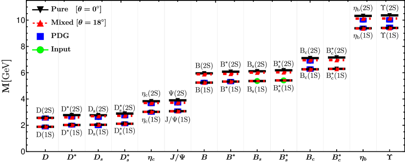
Figure 2: The mass spectra of the ground $(1S)$ and first radial excited $(2S)$ states of the mesons in pure ($\theta=0^{\circ}$) and mixed ($\theta=18^{\circ}$) configurations shown as solid-black and red-dashed lines, respectively. The comparison is made with experimental data from PDG represented by blue squares PDG2022 .

III Applications

In this section, we provide a concise overview of the calculations involved in determining additional observables to assess the predictivity of the present study. These observables include pseudoscalar and vector decay constants and DAs, electromagnetic form factors, charge radii, transition form factors of quarkonia, as well as di-leptonic decays of heavy-light mesons.

III.1 Decay Constants and Distribution Amplitudes

The precise determination of the pseudoscalar and vector decay constants is crucial as they encapsulate the internal structure of hadrons. The pseudoscalar meson decay constant $(f_{P})$ and vector meson decay constant $(f_{V})$ can be expressed in terms of the parametrization of the weak current matrix elements of the meson and the vacuum. Accordingly, the decay constants for pseudoscalar and vector mesons are defined as follows Ball:1998sk ; Ahmady:2019hag ; Gurjar:2024wpq

$$\left<0|\bar{q}(0)\gamma^{\mu}\gamma_{5}{q}(0)|P\right>=if_{P}\ P^{\mu},$$ (18)

for pseudoscalar meson and

$$\left<0|\bar{q}(0)\gamma^{\mu}{q}(0)|V(P,\lambda)\right>=f_{V}\ M_{V}~{}\epsilon_{\lambda}^{\mu},$$ (19)

for a vector meson with longitudinal $(\lambda=0)$ polarization. Here, $q(\bar{q})$ represent the field operators for quark (anti-quark) located at the same space-time points and $M_{V}$ denotes the mass of the vector meson.

The calculation of decay constants can be facilitated by employing the plus component $(\mu=+)$ of the current. The explicit expressions for the decay constants of the $nS$ state pseudoscalar and vector mesons are given by Choi2021 ; Choi2014 ; Choi:2007yu .

$$f^{nS}_{{P}{(V)}}=2\sqrt{6}\int_{0}^{1}dx\int\frac{d^{2}\textbf{k}_{\bot}}{16\pi^{3}}\frac{\Phi_{nS}\left(x,\textbf{k}_{\bot}\right)}{\sqrt{\mathcal{A}^{2}+{\textbf{k}^{2}_{\bot}}}}\mathcal{O}_{P(V)},\,$$ (20)

where $\mathcal{O}_{P}=\mathcal{A}$ and $\mathcal{O}_{V}$ = $\mathcal{A}$ + $\frac{2{\textbf{k}^{2}_{\bot}}}{\textbf{D}_{LF}}$ with definitions $\mathcal{A}=(1-x)m_{q}+x\,m_{\bar{q}}$ and $\textbf{D}_{LF}$ = $M_{0}+m_{q}+m_{\bar{q}}$. Indeed, the decay constants have been demonstrated to be independent of the current component and polarization; further detailed analysis on this topic can be found in Choi2021 ; Choi2014 .

In this work, although the distribution amplitudes derived from various components of the currents and polarization vectors result in distinct classifications by twists, our analysis will specifically concentrate on the twist-2 DAs. The twist-2 quark DAs can be obtained from Eq. (20) as Choi:2007yu

$$\phi^{nS}_{P(V)}(x)=\frac{2\sqrt{6}}{f^{nS}_{P(V)}}\int\frac{d^{2}\textbf{k}_{\bot}}{(2\pi)^{3}}\frac{\Phi_{nS}\left(x,\textbf{k}_{\bot}\right)}{\sqrt{\mathcal{A}^{2}+{\textbf{k}^{2}_{\bot}}}}\mathcal{O}_{P(V)},\,$$ (21)

so that it can be normalized as

$$\int_{0}^{1}{{\phi}}^{nS}_{P(V)}\,(x)\,dx=1.$$ (22)

The expectation value of the longitudinal momentum, given by $\xi\,=\,x-\,(1-x)\,=\,2x-1$ and known as $\xi$-moments is expressed as follows Choi:2007yu

$$\langle\xi^{m}\rangle_{nS}=\int_{0}^{1}\mathrm{d}x\xi^{m}{\phi}^{nS}_{P(V)}\,(x).\,$$ (23)

III.2 Electromagnetic and Transition Form Factors

The electromagnetic form factor of a pseudoscalar meson is calculated in the Drell-Yan-West frame where $q^{+}\,=q^{0}+q^{3}=0$ with $\textbf{q}^{2}_{\bot}\,=Q^{2}\,=-q^{2}$. In this frame, using the $+$ component of the current, the form factor can be derived as $F_{\rm em}(Q^{2})=\frac{\langle P^{\prime}|J^{+}|P\rangle}{2P^{+}}$ with the explicit form provided by Choi1999

$$F^{nS}_{\rm em}(Q^{2}) = e_{q}\int_{0}^{1}dx\int\frac{d^{2}\textbf{k}_{\bot}}{16\pi^{3}}\Phi_{nS}\left(x,\textbf{k}_{\bot}\right)\Phi^{*}_{nS}\left(x,\textbf{k}^{\prime}_{\bot}\right)$$

$$\times\frac{\mathcal{A}^{2}+\,{\textbf{k}_{\bot}}\cdot{\textbf{k}^{\prime}_{\bot}}}{\sqrt{\mathcal{A}^{2}+{\textbf{k}^{2}_{\bot}}}\sqrt{\mathcal{A}^{2}+{\textbf{k}^{{}^{\prime}2}_{\bot}}}}+e_{\bar{q}}(m_{q}\leftrightarrow m_{\bar{q}}),$$

where $e_{q}(e_{\bar{q}})$ is the electric charge of quark (anti-quark) and $\textbf{k}^{\prime}_{\bot}={\textbf{k}_{\bot}}+\left(1-x\right){\textbf{q}_{\bot}}$. The EMFF is normalized such that $F_{\rm em}\left(0\right)\,=\,e_{q}\,+\,e_{\bar{q}}$ and the charge radius is computed as

$$\langle r^{2}\rangle_{nS}=-6\,\frac{dF^{nS}_{\rm em}(Q^{2})}{dQ^{2}}\bigg{\rvert}_{Q^{2}\,=\,0}.$$ (25)

The transition form factors $F_{P\gamma}$ for the $P\to\gamma^{*}\gamma$ transition can be derived from the matrix element of electromagnetic current as

$$\langle\gamma(P-q)|J^{\mu}|P(P)\rangle=ie^{2}F_{P\gamma}(Q^{2})\epsilon^{\mu\nu\rho\sigma}P_{\nu}\varepsilon_{\rho}q_{\sigma},$$ (26)

where $P^{\mu}$ and $q^{\mu}$ are the four momenta of the incident pseudoscalar meson and virtual photon, respectively and $\varepsilon$ is the transverse polarization vector of the final (on-shell) photon.

In Refs. Ryu:2018egt ; Choi:2017pi , the TFFs were obtained from both $q^{+}=0$ frame and $q^{+}=P^{+}$ frame and were demonstrated to be independent of the choice of reference frame. Moreover, the authors showed that the result obtained from the $q^{+}=P^{+}$ frame exhibit a salient feature that distinguishes it from those derived from the $q^{+}=0$ frame. This notable advantage of the $q^{+}=P^{+}$ frame not only confirms the boost invariance of the results but also facilitates a more effective computation of the timelike form factor compared to the commonly used $q^{+}=0$ frame.

The explicit form of the TFFs for the $nS$ state heavy quarkonina $\eta_{c(b)}\to\gamma^{*}\gamma$ transition in the $q^{+}=P^{+}$ frame is provided by Ryu:2018egt ; Choi:2017pi

$$F^{nS}_{\eta_{c(b)}\gamma}(q^{2})= e_{c(b)}^{2}\frac{\sqrt{2N_{c}}}{4\pi^{3}}\int_{0}^{1}\frac{{\rm d}x}{(1-x)}\int{\rm d}^{2}{\bf{k}_{\perp}}\frac{1}{M_{0}^{2}-q^{2}}$$

$$\times\Psi^{nS}_{\frac{\uparrow\downarrow-\downarrow\uparrow}{\sqrt{2}}}(x,\bf{k}_{\perp}),$$ (27)

with $N_{c}=3$ is the number of colors. The LFWF $\Psi_{\frac{\uparrow\downarrow-\downarrow\uparrow}{\sqrt{2}}}(x,\bf{k}_{\perp})$ of a heavy quarkonia where quark and antiquark masses are equal $m_{Q}=m_{\bar{Q}}$ is defined as Ryu:2018egt ; Choi:2017pi

$$\Psi^{nS}_{\frac{\uparrow\downarrow-\downarrow\uparrow}{\sqrt{2}}}(x,\mathbf{k}_{\perp})=\frac{m_{Q}}{\sqrt{\mathbf{k}_{\perp}^{2}+m_{Q}^{2}}}\Phi_{nS}(x,\mathbf{k}_{\perp}).$$ (28)

We should note that the direct calculation of the timelike TFF is particularly effective due to the the simple pole structure $(M^{2}_{0}-q^{2})^{-1}$ in the timelike region ($q^{2}>0$). By performing analytic continuation from timelike region ($q^{2}>0$) to spacelike region ($q^{2}\to-q^{2}$), the TFF can be determined in the spacelike region ($Q^{2}=-q^{2}$) without singularities.

III.3 Di-leptonic Decays

The charged pseudoscalar mesons $B^{+}$, $D^{+}$ and $D_{s}^{+}$ can undergo annihilation through a $W^{\pm}$ boson into a lepton-neutrino pair $(l^{+}\nu_{l})$. The presence of highly energetic leptons in the final states makes these decays experimentally prominent, while the absence of hadrons in the final state renders these decays theoretically clean to predict, depending only on a single hadronic parameter: the pseudoscalar decay constant villa2007 . Assuming that the main contribution to these weak leptonic decay transitions comes from the virtual boson-mediated annhilation of the bound quark-antiquark pair $(q_{1}\bar{q_{2}})$ inside the pseudoscalar meson $\mathcal{P}$, the partial decay width is given by  villa2007 ; PDG2022 ; rosner2008

$$\Gamma(\mathcal{P}^{+}\rightarrow l^{+}\nu_{l})=\frac{G_{F}^{2}}{8\pi}f^{2}_{\mathcal{P}}|V_{{q_{1}}{q_{2}}}|^{2}m_{l}^{2}\left(1-\frac{m_{l}^{2}}{M^{2}_{\mathcal{P}}}\right)^{2}M_{\mathcal{P}}\,,$$ (29)

where $M_{\mathcal{P}}$ and $f_{\mathcal{P}}$ denote the mass and the decay constant of a ground state pseudoscalar meson, respectively. Our predicted values of $M_{\mathcal{P}}$ and $f_{\mathcal{P}}$ are being used in the computation of these transitions. The values of other parameters such as Fermi’s coupling constant $G_{F}=1.16\times 10^{-5}$ GeV^-2, mass of leptons as $m_{e}=0.0005$ GeV, $m_{\mu}=0.105$ GeV, $m_{\tau}=1.776$ GeV, CKM matrix elements $V_{ub}=(3.8\pm 0.20)\times 10^{-3}$, $V_{cd}=0.221\pm 0.004$ and $V_{cs}=0.975\pm 0.006$ are taken from PDG PDG2022 . The branching ratio for these transitions is then obtained as

$$\mathcal{B}=\Gamma_{(\mathcal{P^{+}}\rightarrow l^{+}\nu_{l})}\times\tau_{\mathcal{P}}$$ (30)

where $\tau_{\mathcal{P}}$ is lifetime of the respective mesons. We take $\tau_{D^{+}}$ = $1.033\times 10^{-12}$ s, $\tau_{D_{s}^{+}}$ = $0.501\times 10^{-12}$ s and $\tau_{B^{+}}$ = $1.638\times 10^{-12}$ s as listed in PDG PDG2022 .

The di-leptonic decay of neutral $B_{q}^{0}$ mesons into two charged lepton pairs $(l^{+}l^{-})$ is suppressed by Glashow-Iliopoulous-Maiani (GIM) mechanisms and helicity constraints. However, such transitions occur through higher-order diagrams involving flavour-changing neutral currents. The presence of higher-order interaction vertices significantly reduces its decay probability. Thus, this class of di-leptonic decays are known as rare decays. The decay width for these transitions in neutral charge mesons is expressed as bobeth2014 ; bobeth20142 ; buchalla1993

$$\Gamma_{(B^{0}_{q}\rightarrow\ell^{+}\ell^{-})} = \frac{G_{F}^{2}}{\pi}\frac{\alpha^{2}f^{2}_{B_{q}}m_{\ell}^{2}}{(4\pi\sin^{2}\Theta_{W})^{2}}\ m_{B_{q}}$$

$$\sqrt{1-4\frac{m_{\ell}^{2}}{m_{B_{q}}^{2}}}|V_{tb}^{*}V_{tq}|^{2}|C_{10}|^{2}$$

where the Weinberg angle is approximated as $\Theta_{W}(\approx 28^{\circ})$ lee2015 . The PDG values for CKM matrix elements $V_{tb}$, $V_{td}$ and $V_{ts}$ as $1.014\pm 0.029$, $(8.6\pm 0.2)\times 10^{-3}$ and $(41.5\pm 0.9)\times 10^{-3}$ respectively are considered PDG2022 . Within the Standard Model, rare decays are predominantly governed by the operator $\mathcal{O}_{10}$ with the corresponding Wilson coefficient $C_{10}$ given as buchalla1993 ; buras1998

$$C_{10}=\eta_{Y}\frac{x_{t}}{8}\left[\frac{x_{t}-4}{x_{t}-1}+\frac{3x_{t}}{(x_{t}-1)^{2}}\ln x_{t}\right]$$ (32)

with $x_{t}=(m_{t}/m_{W})^{2}$; $m_{t}$ = 172.57 GeV and $m_{W}$ = 80.36 GeV PDG2022 . The $\eta_{Y}=1.026$ is the next leading order corrections buras1998 . The branching ratio for rare transitions is given by

$$\mathcal{B}=\Gamma_{(B^{0}_{q}\rightarrow\ell^{+}\ell^{-})}\times\tau_{B_{q}^{0}}$$ (33)

We take experimental values $\tau_{B^{0}}$ = $(1.517\pm 4)\times 10^{-12}$ s and $\tau_{B_{s}^{0}}$ = $(1.527\pm 0.0011)\times 10^{-12}$ s PDG2022 .

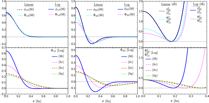
Figure 3: Upper Panel: Comparison of the pure ($\phi$) and mixed ($\Phi$) radial wave functions for $1S$ and $2S$ states of bottomonium ($b\bar{b}$) from present study and those obtained by linear confining potential Arifi2022 . It is noticed that $2S$ wave function has sizable mixing effect whereas $1S$ wave function has marginal modification. Lower Panel: The radial wave functions $\Phi_{1S}$ and $\Phi_{2S}$ for the various bottom flavoured mesons for mixed case.

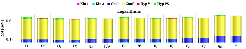
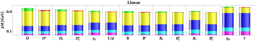
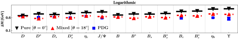
Figure 4: The upper panel shows the various component contribution to the mass gap $(\Delta M)$ from the present study with the logarithmic confinement whereas the middle panel presents the same with linear confinement from Ref.  Arifi2022 . The Kin 1 and Kin 2 represents the heavier and light quark contribution to kinetic energy respectively. The red segment is considered as a subtracted part to the total mass gap since hyperfine vector contribution is negative. The lower panel shows the total mass gap from pure (solid-black) and mixed (red-dashed) configurations for $1S$ and $2S$ states where comparison is made with PDG quoted values (blue-squares)  PDG2022 .

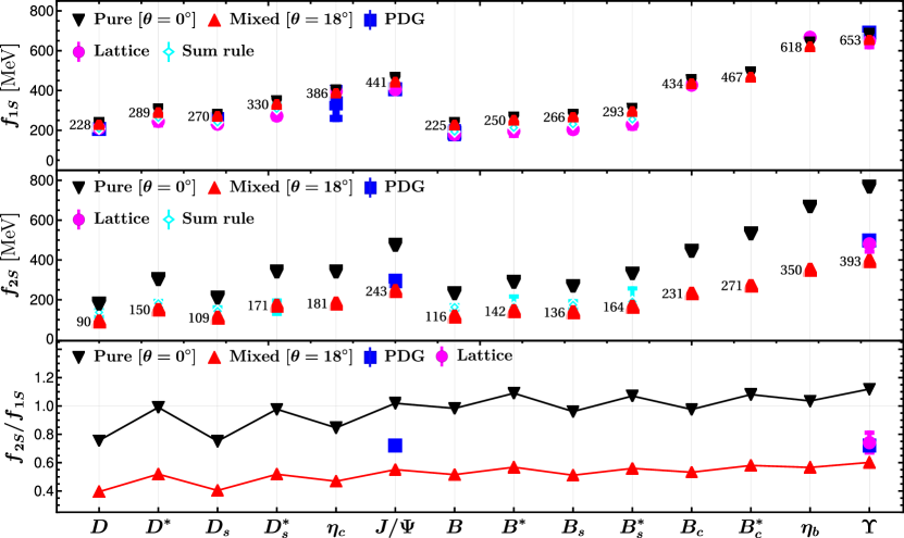
Figure 5: The predicted decay constant of the $1S$ and $2S$ states of vector and pseudoscalar states. The results are compared with experimental values listed by PDG PDG2022 , available lattice simulations Hatton2020 ; Hatton2021 ; Aoki2022 and SumRule prediction Bevcirevic2014 ; Veliev2011 ; Narison2002 ; Wang2015 .

Table 2: Ground state mass spectra of mesons (All are in units of MeV).

State	Pure	Mixed $(18^{\circ})$	PDG PDG2022	Linear Arifi2022	Linear Mixed $(12^{\circ})$ Arifi2022	Exponential Dhiman2019	GI Godfrey1985	RQM Ebert:2002pp ; Ebert:2009ua
$\Upsilon(1S)$	9410	9390	9460.40 $\pm$ 0.10	9485	9480	…	9460	9460
$\eta_{b}(1S)$	9381	9362	9398.7 $\pm$ 2.0	9399	9399	…	9400	9400
$\Upsilon(2S)$	10365	10126	10023.4 $\pm$ 0.5	10377	10175	…	10000	10023
$\eta_{b}(2S)$	10322	10114	9999 $\pm$ 4	10249	10123	…	9980	9993
$B^{*}_{c}(1S)$	6295	6285	…	6343	6340	…	6340	6332
$B_{c}(1S)$	6262	6252	6274.47 $\pm$ 0.32	6269	6270	…	6270	6270
$B^{*}_{c}(2S)$	7159	6961	…	7059	6930	…	6890	6881
$B_{c}(2S)$	7110	6948	6871.2 $\pm$ 1.0	6948	6885	…	6850	6835
$B^{*}_{s}(1S)$	5416	5416	5415.4${}^{+1.8}_{-1.5}$	5421	5418	5329	5450	5414
$B_{s}(1S)$	5366	5366	5366.92 $\pm$ 0.10	5325	5330	5313	5390	5392
$B^{*}_{s}(2S)$	6186	6026	…	6067	5987	…	6010	5992
$B_{s}(2S)$	6111	6006	…	5924	5928	…	5980	5976
$B^{*}(1S)$	5325	5327	5324.71 $\pm$ 0.21	5325	5325	5242	5370	5326
$B(1S)$	5242	5247	5279.34 $\pm$ 0.12	5174	5182	5212	5310	5272
$B^{*}(2S)$	6075	5913	…	5968	5886	…	5930	5906
$B(2S)$	5951	5881	5869 $\pm$ 9 2	5740	5794	…	5900	5890
$J/{\Psi}(1S)$	3072	3065	3096.900 $\pm$ 0.006	3090	3087	…	3100	3096
$\eta_{c}(1S)$	3023	3017	2983.9 $\pm$ 0.4	2987	2990	…	2970	2979
${\Psi}(2S)$	3901	3714	3686.10 $\pm$ 0.06	3781	3670	…	3680	3686
$\eta_{c}(2S)$	3828	3694	3637.7 $\pm$ 1.1	3627	3608	…	3620	3588
$D^{*}_{s}(1S)$	2121	2121	2112.2 $\pm$ 0.4	2113	2111	1971	2130	2111
$D_{s}(1S)$	2037	2040	1968.35 $\pm$ 0.07	1938	1946	1929	1980	1969
$D^{*}_{s}(2S)$	2891	2723	2714 $\pm$ 5	2798	2706	…	2730	2731
$D_{s}(2S)$	2765	2690	2591 $\pm$ 6 3	2546	2600	…	2670	2688
$D^{*}(1S)$	2022	2025	$2010.26\pm 05$	2020	2017	1884	2040	2010
$D(1S)$	1884	1891	$1869.66\pm 05$	1731	1745	1803	1880	1871
$D^{*}(2S)$	2774	2600	$2627\pm 10$	2714	2608	…	2640	2632
$D(2S)$	2568	2545	$2549\pm 19$	2282	2432	…	2580	2581

• From the observation by LHC_b Collaboration in $B$ mesons LHCb2015 .

• From the recent observation by LHC_b Collaboration in $D_{s}$ mesons Lhcb2021ds .

Table 3: Decay constant of heavy-heavy mesons (All are in units of MeV).

	$f_{\Upsilon}(1S)$	$f_{\eta_{b}}(1S)$	$f_{J/\psi}(1S)$	$f_{\eta_{c}}(1S)$	$f_{B^{*}_{c}}(1S)$	$f_{B_{c}}(1S)$	References
Pure	686	646	465	403	494	455	This work
Mixed $\left(\theta=18^{\circ}\right)$	653	618	441	386	467	434	This work
PDG	689 $\pm$ 5	…	407 $\pm$ 5	335 $\pm$ 75	…	…	PDG2022
BLFQ	532	574	379	423	…	…	Li2016
LFQM	611	605	361	353	391	389	Choi2015
LFQM (pure)	688	647	403	356	436	406	Arifi2022
LFQM $(\theta=12^{\circ})$	666	629	390	347	421	393	Arifi2022
Lattice (HPQCD)	677.2 $\pm$ 9.7	724 $\pm$ 24	410 $\pm$ 17	…	422 $\pm$ 13	434 $\pm$ 15	McNeile:2012qf ; Donald:2012ga ; Davies:2010ip ; Colquhoun:2014ica ; Becirevic:1998ua
Lattice $n_{f}$ =2	…	…	418 $\pm$ 8	387 $\pm$ 7	…	…	Bailas2018
BS	422	472	304	278	305	312	Chen2019
PM (Linear)	706	744	338	363	435	465	Patel2009
QCDSR	…	251 $\pm$ 72	401 $\pm$ 46	309 $\pm$ 39	…	320 $\pm$ 95	Bevcirevic2014 ; Veliev2011
	$f_{\Upsilon}(2S)$	$f_{\eta_{b}}(2S)$	$f_{J/\psi}(2S)$	$f_{\eta_{c}}(2S)$	$f_{B^{*}_{c}}(2S)$	$f_{B_{c}}(2S)$	References
Pure	768	669	474	341	534	444	This work
Mixed $\left(\theta=18^{\circ}\right)$	393	350	243	181	271	231	This work
Pure	771	671	420	318	477	407	Arifi2022
Mixed $\left(\theta=12^{\circ}\right)$	498	443	274	214	308	268	Arifi2022
PDG	497$\pm$5	…	294 $\pm$ 5	…	…	…	PDG2022
BLFQ	518 $\pm$ 48	524 $\pm$ 58	312 $\pm$ 73	299 $\pm$ 68	…	…	Li2017

Table 4: Decay constant of heavy-light mesons (All are in units of MeV).

	$f_{B^{*}}(1S)$	$f_{B}(1S)$	$f_{B^{*}_{s}}(1S)$	$f_{B_{s}}(1S)$	$f_{D^{*}}(1S)$	$f_{D}(1S)$	$f_{D^{*}_{s}}(1S)$	$f_{D_{s}}(1S)$	References
Pure	267	238	312	281	307	238	350	282	This work
Mixed $(\theta=18^{\circ})$	250	225	293	266	289	228	330	270	This work
BLFQ	202 $\pm$ 3	233 $\pm$ 50	230 $\pm$ 36	259 $\pm$ 54	281 $\pm$ 20	295$\pm$ 63	306 $\pm$ 39	313 $\pm$ 67	Tang:2019gvn
FLAG $N_{f}$ = 4	…	190.0 $\pm$ 1.3	…	230.3 $\pm$ 1.3	…	212.0 $\pm$ 0.7	…	249.9 $\pm$ 0.5	Aoki2022
QL (Taiwan)	…	…	…	…	…	235 $\pm$ 8	…	266 $\pm$ 10	Chiu2005
LFQM (pure)	215	196	256	235	265	212	303	251	Arifi2022
LFQM $(\theta=12^{\circ})$	208	190	247	228	257	208	294	246	Arifi2022
LFQM	172	163	194	184	230	197	253	219	Dhiman2019
LFQM	185	181	216	205	230	208	260	232	Choi2015
BS	238 $\pm$ 18	196 $\pm$ 29	272 $\pm$ 20	216 $\pm$ 32	340 $\pm$ 23	230 $\pm$ 25	375 $\pm$ 24	248 $\pm$ 27	cvetivc2004
BS	…	193	…	195	…	238	…	241	wang2004
QCDSR	…	203 $\pm$ 23	…	236 $\pm$ 30	…	203 $\pm$ 23	…	235 $\pm$ 24	Narison2002
QCDSR	213 $\pm$ 18	194 $\pm$ 15	255 $\pm$ 19	231 $\pm$ 16	263 $\pm$ 12	208 $\pm$ 10	308 $\pm$ 21	240 $\pm$ 10	Wang2015
RQM	219	189	251	218	310	234	315	268	Ebert2006
	$f_{B^{*}}(2S)$	$f_{B}(2S)$	$f_{B^{*}_{s}}(2S)$	$f_{B_{s}}(2S)$	$f_{D^{*}}(2S)$	$f_{D}(2S)$	$f_{D^{*}_{s}}(2S)$	$f_{D_{s}}(2S)$	References
Pure	291	234	334	270	304	180	342	212	This work
Mixed $(\theta=18^{\circ})$	142	116	164	136	150	90	171	109	This work
Pure	236	197	276	232	266	168	301	200	Arifi2022
Mixed $(\theta=12^{\circ})$	149	126	176	150	171	110	195	133	Arifi2022
RQM	…	…	…	…	293	292	…	…	Shah2016bbs

Table 5: The first six $\xi$ moments for the mixed $1S$ and $2S$ states of mesons.

	$\Upsilon(1S)$	$\eta_{b}(1S)$	$J/\psi(1S)$	$\eta_{c}(1S)$	$B_{c}^{*}(1S)$	$B_{c}(1S)$	${B^{*}}(1S)$	${B}(1S)$	${B^{*}_{s}}(1S)$	${B_{s}}(1S)$	${D^{*}}(1S)$	${D}(1S)$	${D^{*}_{s}}(1S)$	${D_{s}}(1S)$
$\langle\xi^{1}\rangle$	…	…	…	…	0.378	0.378	0.607	0.604	0.580	0.579	0.311	0.301	0.270	0.267
$\langle\xi^{2}\rangle$	0.047	0.047	0.095	0.098	0.196	0.197	0.412	0.409	0.383	0.383	0.213	0.212	0.189	0.192
$\langle\xi^{3}\rangle$	…	…	…	…	0.111	0.112	0.299	0.297	0.272	0.272	0.132	0.132	0.106	0.108
$\langle\xi^{4}\rangle$	0.005	0.005	0.020	0.022	0.068	0.069	0.228	0.227	0.204	0.204	0.099	0.100	0.078	0.081
$\langle\xi^{5}\rangle$	…	…	…	…	0.044	0.044	0.180	0.180	0.158	0.159	0.073	0.075	0.054	0.057
$\langle\xi^{6}\rangle$	0.001	0.001	0.006	0.006	0.029	0.030	0.147	0.146	0.125	0.127	0.059	0.061	0.042	0.044
	$\Upsilon(2S)$	$\eta_{b}(2S)$	$J/\psi(2S)$	$\eta_{c}(2S)$	$B_{c}^{*}(2S)$	$B_{c}(2S)$	${B^{*}}(2S)$	${B}(2S)$	${B^{*}_{s}}(2S)$	${B_{s}}(2S)$	${D^{*}}(2S)$	${D}(2S)$	${D^{*}_{s}}(2S)$	${D_{s}}(2S)$
$\langle\xi^{1}\rangle$	…	…	…	…	0.259	0.245	0.380	0.339	0.366	0.332	0.002	-0.168	0.028	-0.081
$\langle\xi^{2}\rangle$	0.093	0.098	0.180	0.208	0.154	0.151	0.158	0.114	0.165	0.131	0.073	0.010	0.132	0.119
$\langle\xi^{3}\rangle$	…	…	…	…	0.097	0.098	0.064	0.024	0.083	0.055	0.009	-0.047	0.051	0.034
$\langle\xi^{4}\rangle$	0.014	0.015	0.050	0.060	0.069	0.071	0.020	-0.014	0.047	0.025	0.020	-0.013	0.060	0.061
$\langle\xi^{5}\rangle$	…	…	…	…	0.050	0.052	-0.001	-0.030	0.030	0.012	0.010	-0.016	0.041	0.042
$\langle\xi^{6}\rangle$	0.003	0.003	0.017	0.021	0.037	0.040	-0.011	-0.035	0.021	0.008	0.012	-0.005	0.039	0.044

Table 6: The charge radii $\langle r^{2}\rangle$ of mixed 1S and 2S pseudoscalar mesons (All are in units of fm²).

	$\eta_{b}(1S)$	$\eta_{c}(1S)$	$B_{c}^{+}(1S)$	${B^{0}}(1S)$	${B^{+}}(1S)$	${B_{s}^{0}}(1S)$	${D^{0}}(1S)$	${D^{+}}(1S)$	${D_{s}^{+}}(1S)$	References
This work	0.009	0.039	0.032	-0.125	0.246	-0.067	-0.231	0.144	0.085
LFQM	0.010	0.042	0.036	-0.155	0.314	-0.080	-0.282	0.171	0.095	Arifi2022
BLFQ	0.012	0.027	…	…	…	…	…	…	…	Li2017
LFQM	…	…	0.043	-0.187	0.378	-0.119	-0.304	0.184	0.124	Hwang2002
CCQM	…	…	…	…	…	…	…	0.255	0.142	Moita2021
Lattice	…	0.063	…	…	…	…	…	…	…	Dudek2006
Lattice (L)	…	…	…	…	…	…	…	0.138(13)	…	Can:2012tx
Lattice (Q)	…	…	…	…	…	…	…	0.152(26)	…	Can:2012tx
Lattice (B1)	…	0.052(4)	…	…	…	…	…	0.162(49)	0.082(13)	Li:2017eic ; Li:2020gau
Lattice (C1)	…	0.044(4)	…	…	…	…	…	0.176(69)	0.125(13)	Li:2017eic ; Li:2020gau
	$\eta_{b}(2S)$	$\eta_{c}(2S)$	$B_{c}^{+}(2S)$	${B^{0}}(2S)$	${B^{+}}(2S)$	${B_{s}^{0}}(2S)$	${D^{0}}(2S)$	${D^{+}}(2S)$	${D_{s}^{+}}(2S)$
This work	0.035	0.118	0.115	-0.387	0.725	-0.214	-0.695	0.432	0.252
LFQM	0.030	0.129	0.118	-0.450	0.911	-0.222	-0.801	0.464	0.266	Arifi2022
BLFQ	0.050	0.120	…	…	…	…	…	…	…	Li2017

IV Results and Discussion

In the present study we have computed the ground state masses of heavy-heavy and heavy-light mesons within the LFQM employing the logarithmic confinement potential. The computed spectroscopic results are compared with the values listed by PDG PDG2022 and previous LFQM model predictions based on linear confinement Arifi2022 and exponential confinement Dhiman2019 . Additionally, comparisons are made with the GI model Godfrey1985 and the relativistic quark model (RQM) Ebert:2002pp ; Ebert:2009ua in Table LABEL:Tab:mass_spectra. We attempt to determine the variational parameters and quark masses that can systematically describe all mesons with different $q\bar{q}$ content, rather than the fine tunning of the spectra. As mentioned previously, we employ the experimental values for the $B_{s}^{*}(1S)$ and $B_{s}(1S)$ states provided by the PDG as input. The masses for other states are our model predictions. Notably, we observe that the calculated masses are found to be close to the experimental values of the respective states.

In Fig. 2, we show the mass spectra of the 1S and 2S state heavy mesons for both pure ($\theta=0^{\circ}$) and mixed ($\theta=18^{\circ}$) configurations. The black solid line with down-triangles represents the model predictions for logarithmic confinement without the inclusion of mixing effects, while the red dot-dashed line with up-triangles represents predictions after considering the mixing effect. The experimental values listed by the PDG PDG2022 are shown with blue rectangles. The green disks represent the input masses from the PDG used to fix the model parameters. Our findings clearly demonstrate that the spectroscopic results with mixing are more close to the existing experimental values listed in PDG PDG2022 . The impact of mixing appears more noticeable in the $2S$ states compared to $1S$ states.

The LHC_b Collaboration has put forward both the natural $(0^{-},1^{+},2^{-},...)$ and unnatural $(0^{+},1^{-},2^{+},...)$ parity possibilities for the newly observed resonances $B_{J}(5840)$ and $B_{J}(5960)$ LHCb2015 ; PDG2022 . The average mass of 5869 $\pm$ 9 MeV for $B_{J}(5840)$ excludes its identification as a higher orbital excited state  LHCb2015 ; PDG2022 . Therefore, we are left with two possible assignments, $B(2S)$ and $B^{*}(2S)$, for $B_{J}(5840)$. Our prediction of $B(2S)$ as 5881 MeV is found to be comparable to the average measured mass of $B_{J}(5840)$. Hence, we identify $B_{J}(5840)$ as the $B(2S)$ state of the $B$ family. We note that considering $B_{J}(5960)$ as $B^{*}(2S)$ with a measured mass of 5969.2$\pm$ 2.9 MeV gives hyperfine splitting $M(2^{3}S_{1})-M(2^{1}S_{0})$ of approximately 100 MeV. This is higher than the well-established ground state hyperfine splitting $M(1^{3}S_{1})-M(1^{1}S_{0})$ of 45 MeV in $B$ mesons. This contradicts the typical expectation that the hyperfine splittings between the radially excited states should be lower than those between the ground states. Moreover, this consideration also violates the hierarchy $\Delta M_{P}>\Delta M_{V}$. Hence, from present study, we could identify $B_{J}(5840)$ as $B(2S)$. However, further experimental investigation and analysis may be necessary to reconcile the current understanding of the $2S$ states for heavy-light mesons. Also, the state $D_{s0}(2590)$ with a mass of 2591 $\pm$ 6 MeV was observed in $B^{0}\rightarrow D^{-}D^{+}K^{+}\pi^{-}$ channel, decaying to $D^{+}K^{+}\pi^{-}$ final state by LHC_b Lhcb2021ds . Given that the $K^{+}\pi^{-}$ system belongs to the $S$ wave below the $K^{*}(892)^{0}$ threshold, it indicates that only the unnatural parity states decay to $D^{+}K^{+}\pi^{-}$ Lhcb2021ds . These characteristics increases its identification as $D_{s}(2S)$. Although our predicted mass of 2690 MeV differs by roughly 100 MeV from the measured mass of $D_{s0}(2590)$, it still supports its identification as the $D_{s}(2S)$ state of the $D_{s}$ family.

It is also found that each confinement scheme displays a distinct level of predictability, as evidenced by the $\chi^{2}$ analysis. For the linear potential case, the $\chi^{2}$ analysis yields a value of 0.024 and 0.009 for pure and mixed cases, respectively Arifi2022 . However, for the present study, we find the $\chi^{2}$ value of 0.019 for the pure scenario and 0.003 for the mixed one. Both studies suggests the necessity of mixing effects for achieving improved agreement with the experimental data. The predictions from the logarithmic confinement scheme are comparable to those from the linear confinement scheme somewhat even closer to the data in some cases, as illustrated in Table LABEL:Tab:mass_spectra. By comparing LFQM spectroscopic predictions to those from the traditional potential models, such as GI Godfrey1985 and RQM Ebert:2002pp ; Ebert:2009ua , it is found that LFQM predictions are not yet fully fine-tuned. This is because the fixation of model parameters in general hadron spectroscopy refers to the process of determining the values of parameters, including constituent quark masses, coupling constants, potential parameters and other parameters depending on the specific system being considered. These determinations span from the light meson systems, including the pion known as the pseudo-Goldstone boson severely influenced by the chiral symmetry, to the heavy meson systems, including the open charm and bottom mesons described by the heavy quark symmetry. One may separate the analysis of light meson sectors from the analysis of heavy meson sectors, as we focus on the latter in the present work. By adjusting the values of the model parameters to the known ground states of a specific system, the spectra of radially and orbitally excited states are predicted. Some of these models use the so called “canonical” value of the strong coupling constant for heavy quarks, which is approximately $\alpha_{s}$ = 0.2, or other values in the close vicinity of this estimate Lucha1991 . While the models following “soft QCD” takes the value $\alpha_{s}$ = 0.5 to describe light to heavy mesons in a unified manner Godfrey1985 , more successful models utilize the strong “running” coupling constant, taking into account how the strength varies with the changes in the energy scale. The discrepancy between our results and the PDG reported values of ground state masses may partly be attributed to the limitations of the present framework, which does not include fine-tuning of different energy levels specific to each system. As the constituent quarks inside the mesons have a mass difference of the order of hundred MeV, it may be too difficult to accommodate all the mesons with the same potential parameters. Instead of considering the same values of $a$ and $\alpha_{s}$ for all mesons, one may tune them to be flavor- and scale-dependent for further analysis beyond the present work.

Figure 3 illustrates the effects of mixing on the radial wave functions of 1S and 2S meson states. The upper panel compares the pure and mixed radial wave functions of the 1S and 2S states, as well as the ratios of the 2S to 1S states for both pure, $\phi^{2}_{2S}/\phi^{2}_{1S}$, and mixed, $\Phi^{2}_{2S}/\Phi^{2}_{1S}$, states in bottomonium ($b\bar{b}$). Our results are also compared to those obtained from the linear confinement potential case Arifi2022 . The wave functions for $nS$ states increase with an increase in $n$ for both linear and logarithmic potential without mixing effects, implying that the decay constant would increase for larger $n$. This behaviour naively violates the requirement of the aforementioned experimental hierarchies. However, the inclusion of mixing significantly alters the radial wave functions of the 2S states, while the changes in the 1S states are minimal. The lower panel displays the mixed radial wave functions for heavy-heavy ($b\bar{b},b\bar{c}$) and heavy-light ($b\bar{s},b\bar{q}$) quark states obtained from the logarithmic potential. The range of the radial wave function is inversely proportional to the variational parameter $\beta$ Isgur:1988gb ; Faiman:1968js . From Table LABEL:Tab:variational_parameters, it can be observed that bottomonium has the largest value of $\beta$, resulting in a narrower wave function compared to other meson states. Another noticeable observation is that the radial wave functions at the origin are proportional to $\beta$, leading to both the 1S and 2S states of bottomonium having the highest amplitudes at the origin among the meson wave functions. However, the ratios of the 2S to 1S states remain constant, indicating that they are independent of the quark flavor content.

For the analysis of the mass gap, defined as $\Delta M_{P(V)}=M^{2S}_{P(V)}-M^{1S}_{P(V)}$, we decompose it as follows:

$$\Delta M=\Delta M^{{\text{Kin}}}+\Delta M^{{\text{Conf}}}+\Delta M^{{\text{Coul}}}+\Delta M^{{\text{Hyp}}},$$ (34)

where the total mass gap is separated into four distinct contributions: kinetic energy ($\Delta M^{\rm Kin}$), confinement potential ($\Delta M^{\rm Conf}$), Coulomb potential ($\Delta M^{\rm Coul})$ and hyperfine interaction ($\Delta M^{\rm Hyp}$). This decomposition facilitates a detailed analysis in our numerical calculations. In Fig. 4, we present the decomposition of these contributions to the mass gap specifically for the mixed states ($\Phi_{1S},\Phi_{2S}$). The upper panel illustrates the contributions from the mass gap components for the logarithmic potential, while the middle panel shows an analogous taxonomic analysis for the linear potential Arifi2022 for comparison. Here, Kin 1 and Kin 2 represent the kinetic energy contributions from the heavier quark and lighter quark to the kinetic energy, respectively. Although the mass gap $\Delta M$ appears to be almost flavor-independent, its flavour dependency can be reasonably reflected through the relative contributions from $\Delta M^{\text{Kin}}$, $\Delta M^{\text{Coul}}$ and $\Delta M^{\text{hyp}}$. The Kin 1 and Kin 2 contribution is identical for quarkonia, whereas the Kin 2 contribution increases with the mass difference between the constituent quarks in mesons, as one might intuitively anticipate. Moreover, as inferred from Eq. (II), it becomes apparent that $\Delta M^{\text{Coul}}\propto\beta$, indicating that the Coulomb contribution to the mass gap in heavy-light mesons is comparatively less than that in heavy-heavy mesons. This is consistent with the fact that at short distances, the dominant force is the attractive Coulomb interaction, as illustrated by the blue regions in the upper and middle panels of Fig. 4. Indeed, the contributions from the kinetic and Coulomb terms are minimal for a logarithmic potential compared to a linear potential. The confinement contribution $\Delta M^{\text{Conf}}$ has no substantial dependency on $\beta$ (see Eq.(II)) for the logarithmic potential case. This results in an identical confinement contribution for heavy-light and heavy-heavy mesons, making it less comparable for different flavour mesons but more tractable, as indicated by the yellow regions in the upper panel of Fig. 4. It therefore reflects the flavour independence of the logarithmic potential. The confinement contribution to the mass gap associated with a linear potential varies inversely with $\beta$ ($\Delta M^{\text{Conf}}\propto\beta^{-1})$, capturing the dominant confinement forces at larger distances  Arifi2022 . The lower panel shows the mass gap $\Delta M$ between the 1S and 2S meson states. Here, the solid black line and red-dashed line represent our findings for pure and mixed configurations, respectively. The empirical mass constraint $\Delta M_{P}>\Delta M_{V}$ is found to be satisfied only after the inclusion of the mixing.

In the upper panel of Fig. 5, we present our findings for the decay constants of the 1S state with pure $(\theta=0^{\circ})$ and mixed $(\theta=18^{\circ})$ wave functions ,represented by black down triangles and red up triangles, respectively. The similar results for $2S$ states are shown in the middle panel. In both the upper and middle panels, the numerical values indicate the decay constants obtained from the mixing of wave functions. For comparison we also show the available experimental data from PDG  PDG2022 , other theoretical findings from Lattice  McNeile:2012qf ; Donald:2012ga ; Davies:2010ip ; Colquhoun:2014ica ; Becirevic:1998ua and QCDSR Gelhausen:2014jea . Apparently, the decay constants of the $1S$ states exhibit limited sensitivity to mixing effects, whereas those of the $2S$ states demonstrate significant changes. The $2S$ state decay constants, when accounting for mixing effects are found to be closer to other predictions  PDG2022 ; McNeile:2012qf ; Donald:2012ga ; Davies:2010ip ; Colquhoun:2014ica ; Becirevic:1998ua ; Gelhausen:2014jea .

To make a detailed comparison of the numerical results, we include our findings alongside other theoretical model calculations of decay constants for heavy-heavy Li2016 ; Choi2015 ; McNeile:2012qf ; Donald:2012ga ; Davies:2010ip ; Colquhoun:2014ica ; Becirevic:1998ua ; Arifi2022 ; Bailas2018 ; Chen2019 ; Patel2009 ; Bevcirevic2014 ; Veliev2011 ; Li2017 and heavy-light Tang:2019gvn ; Aoki2022 ; Arifi2022 ; Dhiman2019 ; Choi2015 ; cvetivc2004 ; wang2004 ; Narison2002 ; Wang2015 ; Ebert2006 ; Shah2016bbs mesons in Tables 3 and 4, respectively. From Table 3, it is evident that our predicted values for the vector and pseudoscalar meson decay constants of quarkonia and $B_{c}$ mesons are in good agreement with the experimental results PDG2022 . We also notice that, for quarkonia, the condition $f_{1S}>f_{2S}$ is consistent with experimental observations when the mixing of wave functions is taken into account. Additionally, it is seen that results from all LFQM with different confining schemes Arifi2022 ; Dhiman2019 show similar quantitative results to those of the present study. However, predictions from BLFQ Li2016 and Linear potential model Patel2009 are roughly 100 MeV different from all other predictions. A similar pattern is observed for heavy-light mesons in Table 4.

To date, the PDG has only listed $2S$ decay constants for vector quarkonium states. Based on the known experimental values of decay constants, the ratio $f_{2S}/f_{1S}$ must be less than unity. The lower panel presents the ratio $f_{2S}/f_{1S}$ for both pure and mixed scenarios. Except for $D$, $D_{s}$ and $\eta_{c}$, this empirical constraint is found to be violated in the pure case, while it is satisfied for all heavy-light to heavy-heavy mesons in the mixed case. Despite this, our estimations of the ratio are found to somewhat differ from both experimental observations and lattice results. Further experimental measurements of $2S$ state decay constants will be significant to better understand and observe the impact of mixing effects.

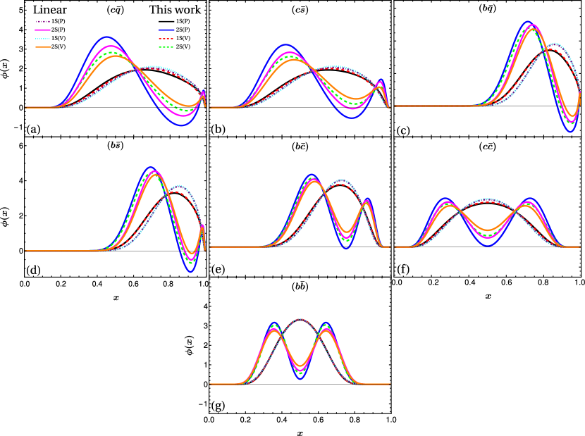
Figure 6: Twist-2 Distribution amplitude of $1S$ and $2S$ pseudoscalar and vector states for the case of mixed configuration with $\theta=18^{\circ}$. The comparison with linear confining potential corresponds to $\theta=12^{\circ}$ also presented Arifi2022 .

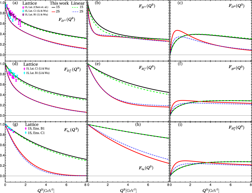
Figure 7: Electromagnetic form factors of the $1S$ and $2S$ pseudoscalar states of mesons with the mixing angle $\theta=18^{\circ}$. The linear confinement potential results with mixing angle $\theta=12^{\circ}$ Arifi2022 and available lattice findings  Can:2012tx ; Li:2017eic ; Li:2020gau are also presented for comparison. For the case of quarkonium only the contribution from quark is considered.

Figure 6 shows the normalized twist-2 quark DAs for vector and pseudoscalar mesons with a mixing angle of $\theta=18^{\circ}$. The solid black and solid blue lines correspond to the $1S$ and $2S$ pseudoscalar mesons, respectively, while the red dashed and green dashed lines represent the $1S$ and $2S$ vector meson states. The DAs without and with the inclusion of mixing effects in the wave function do not show significant differences, so we do not include results with $\theta=0^{\circ}$. For comparison, we also include the results from the linear confining potential Arifi2022 . We follow the traditional convention where the heavier quark inside the mesonic system carries the longitudinal momentum fraction $x$ while the the lighter quark carries the fraction $1-x$. The DAs for the $1S$ pseudoscalar and vector states are not significantly different because the variational parameter $\beta$ is the same for both states within the present formalism. It is noted that the DAs for bottomonium and charmonium exhibit symmetry under the change from $x$ to $1-x$. However, the charmonium DA is found to be wider compared to bottomonium DA due to its lower mass, as expected. Similarly, the extrema for charmonium are shifted more towards the endpoints compared to bottomonium. In the case of heavy-light mesons, as the mass difference between the constituent quark and anti quark inside meson increases, their DAs appear more asymmetrical and sharply peaked. The impact of mass on the DAs can also be noticed from the heavy-light systems. In particular, bottom and bottom-strange mesons have narrower DAs than the charm and charm-strange mesons. We observed similar behavior in the twist-2 DAs compared to those obtained using a linear confining potential. Our predictions show both qualitative and quantitative agreement with these results. It is also apparent from Fig. 6 that the $2S$ pseudoscalar and vector DAs are distinct in contrast to the $1S$ states. This trend is found to be contradictory to the BLFQ results, which indicate that the $1S$ DAs tend to be more distinct Tang:2019gvn . We also find significant difference in the minima of the present DAs compared to the BLFQ outcomes Tang:2019gvn .

Table 5 shows the $\xi$ moments up to $n$ = 6 for vector and pseudoscalar states of $1S$ and $2S$. Due to the same constituent quark masses and symmetrical DAs, the odd-$n$ moments for quarkonium are found to be zero. In the case of heavy-light mesons, due to mass difference between constituent quarks odd-$n$ moments also exhibits the asymmetry. For instance, $\langle\xi^{1}\rangle_{B_{c}(1S)}$, $\langle\xi^{1}\rangle_{B_{s}(1S)}$ and $\langle\xi^{1}\rangle_{B_{q}(1S)}$ are 0.378, 0.579 and 0.604, respectively increasing as the difference between constituents mass increases. The fact that $\langle\xi^{1}\rangle$ of the $D(2S)$ and $D_{s}(2S)$ states is observed to be negative is due to the wide spread of their DAs in the 0 $<$ $x$ $<$ 0.5 domain. Overall, the predictions of $\xi$ moments are in reasonable agreement with the results obtained from the linear potential Arifi2022 .

In Fig. 7, we present the EMFFs of the $1S$ (black) and $2S$ (red) states of heavy-heavy and heavy-light pseudoscalar mesons, respectively. We also illustrate the lattice simulation results for comparison Can:2012tx ; Li:2017eic ; Li:2020gau . For quarkonium, we consider only the contribution from the quarks due to the similar flavour content. It is noted that our predictions for the $1S$ states of $D^{+},~{}D^{+}_{s}$ and $\eta_{c}$ mesons are in good agreement with the lattice results. The form factors of the $2S$ states show a steeper decline compared to the $1S$ states. However, overall one sees a qualitative similarity in the behaviour of the FFs compared to a similar model with linear confinement Arifi2022 . We observe that for heavy-light systems such as $D^{+}$, $D_{s}^{+}$ and $B^{+}$, the dominant contribution to the form factor in the high $Q^{2}$ region comes from the heavy quark whereas the light quark contribution is negligible. Conversely, for the $B_{c}$ meson, both $b$ and $c$ quark contribute equally to the form factors. Table 6 shows the obtained charge radii $\langle r_{nS}^{2}\rangle$ of the pseudoscalar states of heavy-heavy and heavy-light mesons, along with other available predictions Can:2012tx ; Li:2017eic ; Li:2020gau . We find that our results are in relatively good agreement with other model results Li2017 ; Arifi2022 ; Hwang2002 ; Moita2021 .

In Fig. 8, we present the TFFs for charmonium in the spacelike ($Q^{2}<0$) momentum transfer region. The left plot displays the asymptotic behavior for high $Q^{2}$ values. The comparison is made with the experimental data from $BABAR$ BaBar:2010siw along with outcomes from a linear confining potential Arifi2022 . The right panel presents similar results for $2S$ state. The $1S$ state TFFs exhibit similar behaviour for both logarithmic and linear potentials and appear insensitive to mixing effects. The $Q^{2}F_{\eta_{c}\gamma}(Q^{2})$ demonstrates excellent agreement with the experimental data, especially in the region of $Q^{2}<15~{}\text{GeV}^{2}$ for $1S$ state BaBar:2010siw . It is noted that the mixing effects are apparent in $Q^{2}F_{\eta_{c}\gamma}(Q^{2})$ for the $2S$ state.

Figure 9 shows the TFFs for bottomonium in the spacelike momentum transfer region. The line codes are the same as in Fig. 8. Although the qualitative behavior of $F_{\eta_{b}\gamma}$ resembles that of $F_{\eta_{c}\gamma}$, their quantitative characteristics, such as the slope of the form factor at $Q^{2}=0$, differ significantly due to the heavier $b$ quark compared to the $c$ quark. Again, the mixing effects can be seen here for the $2S$ state in $Q^{2}F_{\eta_{b}\gamma}(Q^{2})$. However, the other quantities remain unaffected for the choice of potential and mixing of wave functions. Further experimental measurements can provide more insights and refine our current understanding of TFFs.

The di-leptonic decay widths of the charged pseudoscalar mesons are presented in Table 7. The uncertainty in the prediction of these decay widths from the present study and the linear potential model is due to the uncertainty in the values of CKM matrix elements. The estimated widths for these transitions are approximately twice as large as those reported by ciftci2000 . Also, we note that the large uncertainty in the experimental BRs for some transitions leads to inconclusiveness in the results. However, our predictions for ${\rm Br}(B^{+}\rightarrow e^{+}{\nu_{e}})=(1.30\pm 0.14)\times 10^{-11}$, ${\rm Br}(B^{+}\rightarrow\mu^{+}{\nu_{\mu}})=(5.75\pm 0.60)\times 10^{-7}$, ${\rm Br}(D^{+}\rightarrow e^{+}{\nu_{e}})=(1.02\pm 0.04)\times 10^{-8}$ and ${\rm Br}(D_{s}^{+}\rightarrow e^{+}{\nu_{e}})=(1.45\pm 0.02)\times 10^{-7}$ are in accordance with the experimental BR limits $(<9.8\times 10^{-7})$, $(<8.6\times 10^{-7})$, $(<8.8\times 10^{-6})$ and $(<8.3\times 10^{-5})$, respectively, as quoted by the PDG PDG2022 . We also find that our predictions for ${\rm Br}(B^{+}\rightarrow\tau^{+}{\nu_{\tau}})=(1.29\pm 0.13)\times 10^{-4}$ and ${\rm Br}(D^{+}\rightarrow\tau^{+}{\nu_{\tau}})=(1.76\pm 0.06)\times 10^{-3}$ are close to the experimental values of $(1.09\pm 0.24)\times 10^{-4}$ and $(1.20\pm 0.27)\times 10^{-3}$, respectively.

The rare decays of the charge neutral bottom and bottom-strange mesons by considering the uncertainty persist into the CKM matrix elements are shown in Table 8. Our results for $B^{0}\rightarrow l^{+}l^{-}(l=e,\mu,\tau)$ are consistent with the results of bobeth2014 . The search and analysis of rare decays are challenging experimentally due to the considerably small branching fractions. The large uncertainty associated with the experimental BRs for these processes make it difficult to draw reliable conclusion. However, our predictions for ${\rm Br}(B^{0}\rightarrow e^{+}e^{-})=(3.93\pm 0.41)\times 10^{-15}$ and ${\rm Br}(B_{s}^{0}\rightarrow e^{+}e^{-})=(1.32\pm 0.13)\times 10^{-13}$ fall within the limits of $<3.0\times 10^{-9}$ and $<11.2\times 10^{-9}$, respectively, as measured very recently by LHC_b Aaij2020 . Also, our prediction of ${\rm Br}(B^{0}\rightarrow\mu^{+}\mu^{-})=(1.73\pm 0.18)\times 10^{-10}$ falls within the range of the values listed by LHC_b $(<2.6\times 10^{-10})$ Aaij2022 ; Aaij20221 and CMS $(<3.6\times 10^{-10})$ sirunyan2020 Collaboration. Similarly, our prediction of ${\rm Br}(B_{s}^{0}\rightarrow\mu^{+}\mu^{-})=(5.81\pm 0.58)\times 10^{-9}$ is in excellent agreement with the experimental observation of $(3.09^{+0.46}_{-0.43})\times 10^{-9}$ Aaij2022 ; Aaij20221 reported by LHC_b and $(2.9\pm 0.7\pm 0.2)\times 10^{-10}$ by CMS sirunyan2020 . We also obtain the ratio $\frac{{\rm Br}(B^{0}\rightarrow\mu^{+}\mu^{-})}{{\rm Br}(B_{s}^{0}\rightarrow\mu^{+}\mu^{-})}=0.0298\pm 0.0042$, which is in excellent agreement with the Standard Model prediction of $0.0295^{+0.0028}_{-0.0025}$ bobeth2014 . However, the combined analysis of CMS and LHC_b quotes this ratio as $0.14^{+0.08}_{-0.06}$ that deviates by 2.3$\sigma$ from the standard model prediction CMS:2014xfa ; bobeth2014 . The estimated BR for $B^{0}\rightarrow\tau^{+}\tau^{-}$ and $B_{s}^{0}\rightarrow\tau^{+}\tau^{-}$ are in good agreement with those predicted by bobeth2014 and the experimental data from PDG PDG2022 . We note that weak decays from LFQM with different confinement schemes have predictions close to the measured values of the respective decay channels. However, more detailed analysis on this can be made by evaluating other observables like weak form factors, forward-bakward asymmetry, iso-spin asymmetry and longitudinal and transverse polarization fractions with high $q^{2}$ within LFQM.

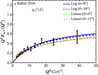
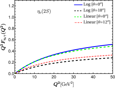
Figure 8: Two photon transition form factors of pseudoscalar states $1S$ and $2S$ of charmonium from logarithmic potential with pure $(\theta=0^{\circ})$ and mixed $(\theta=18^{\circ})$ wave functions. The results obtained from linear confining potential parameters are also presented for pure $(\theta=0^{\circ})$ and mixed $(\theta=12^{\circ})$ cases Arifi2022 . The experimental measurements are from $BABAR$ Collaboration BaBar:2010siw .

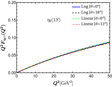
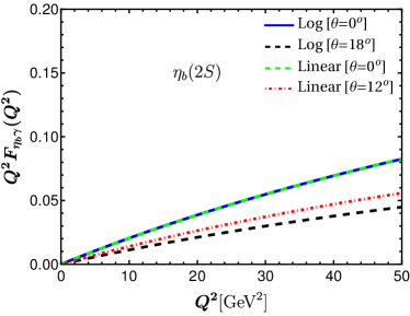
Figure 9: Two photon transition form factors of pseudoscalar states $1S$ and $2S$ of bottomonium from logarithmic potential with pure $(\theta=0^{\circ})$ and mixed $(\theta=18^{\circ})$ wave functions. The results obtained from linear confining potential parameters are also presented for pure $(\theta=0^{\circ})$ and mixed $(\theta=12^{\circ})$ cases Arifi2022 .

Table 7: The branching ratios (in %) for di-leptonic decays of heavy-light mesons. Experimental results are from PDG PDG2022 .

Transition	This Work	Linear Arifi2022	ciftci2000	Experiment PDG2022
	$(\theta=18^{\circ})$	$(\theta=12^{\circ})$
$B^{+}\rightarrow e^{+}{\nu_{e}}$	$(1.30\pm 0.14)\times 10^{-11}$	$(0.91\pm 0.10)\times 10^{-11}$	$\cdots$	$<9.8\times 10^{-7}$
$B^{+}\rightarrow\mu^{+}{\nu_{\mu}}$	$(5.75\pm 0.60)\times 10^{-7}$	$(4.05\pm 0.42)\times 10^{-7}$	4.82 $\times 10^{-7}$	$<8.6\times 10^{-7}$
$B^{+}\rightarrow\tau^{+}{\nu_{\tau}}$	$(1.29\pm 0.13)\times 10^{-4}$	$(0.90\pm 0.09)\times 10^{-4}$	9.25 $\times 10^{-5}$	$(1.09\pm 0.24)\times 10^{-4}$
$D^{+}\rightarrow e^{+}{\nu_{e}}$	$(1.02\pm 0.04)\times 10^{-8}$	$(0.78\pm 0.03)\times 10^{-8}$	…	$<8.8\times 10^{-6}$
$D^{+}\rightarrow\mu^{+}{\nu_{\mu}}$	$(4.47\pm 0.16)\times 10^{-4}$	$(3.42\pm 0.12)\times 10^{-4}$	2.87 $\times 10^{-4}$	$(3.74\pm 0.17)\times 10^{-4}$
$D^{+}\rightarrow\tau^{+}{\nu_{\tau}}$	$(1.76\pm 0.06)\times 10^{-3}$	$(0.13\pm 0.01)\times 10^{-3}$	0.75 $\times 10^{-3}$	$(1.20\pm 0.27)\times 10^{-3}$
$D_{s}^{+}\rightarrow e^{+}{\nu_{e}}$	$(1.45\pm 0.02)\times 10^{-7}$	$(1.15\pm 0.01)\times 10^{-7}$	…	$<8.3\times 10^{-5}$
$D_{s}^{+}\rightarrow\mu^{+}{\nu_{\mu}}$	$(6.39\pm 0.08)\times 10^{-3}$	$(5.05\pm 0.06)\times 10^{-3}$	4.41 $\times 10^{-3}$	$(5.35\pm 0.12)\times 10^{-3}$
$D_{s}^{+}\rightarrow\tau^{+}{\nu_{\tau}}$	$(10.71\pm 0.13)\times 10^{-2}$	$(4.02\pm 0.05)\times 10^{-2}$	4.30 $\times 10^{-2}$	$(5.36\pm 0.10)\times 10^{-2}$

Table 8: The branching ratios (in %) for rare di-leptonic decays of charge neutral heavy-light mesons. Experimental results are from PDGPDG2022 .

Transition	This Work	Linear Arifi2022	bobeth2014	Experiment PDG2022
	$(\theta=18^{\circ})$	$(\theta=12^{\circ})$
$B^{0}\rightarrow e^{+}e^{-}$	$(3.93\pm 0.41)\times 10^{-15}$	$(2.76\pm 0.29)\times 10^{-15}$	$(2.48\pm 0.21)\times 10^{-15}$	$<2.5\times 10^{-9}$
				$<3.0\times 10^{-9}$ Aaij2020 $[LHCb]$
$B^{0}\rightarrow\mu^{+}\mu^{-}$	$(1.73\pm 0.18)\times 10^{-10}$	$(1.22\pm 0.13)\times 10^{-10}$	$(1.06\pm 0.09)\times 10^{-10}$	$<5^{+17}_{-15}\times 10^{-11}$
				$<2.6\times 10^{-10}$ Aaij2022 ; Aaij20221 $[LHCb]$
				$<3.6\times 10^{-10}$ sirunyan2020 $[CMS]$
$B^{0}\rightarrow\tau^{+}\tau^{-}$	$(3.65\pm 0.38)\times 10^{-8}$	$(2.53\pm 0.26)\times 10^{-8}$	$(2.22\pm 0.19)\times 10^{-8}$	$<2.1\times 10^{-3}$
$B_{s}^{0}\rightarrow e^{+}e^{-}$	$(13.19\pm 1.32)\times 10^{-14}$	$(9.62\pm 0.97)\times 10^{-14}$	$(8.54\pm 0.55)\times 10^{-14}$	$<9.4\times 10^{-9}$
				$<11.2\times 10^{-9}$ Aaij2020 $[LHCb]$
$B_{s}^{0}\rightarrow\mu^{+}\mu^{-}$	$(5.81\pm 0.58)\times 10^{-9}$	$(4.24\pm 0.43)\times 10^{-9}$	$(3.65\pm 0.23)\times 10^{-9}$	$(2.9\pm 0.4)\times 10^{-9}$
				$(3.09^{+0.46}_{-0.43}\pm 0.14)\times 10^{-9}$Aaij2022 ; Aaij20221 $[LHCb]$
				$(2.9\pm 0.7\pm 0.2)\times 10^{-10}$sirunyan2020 $[CMS]$
$B_{s}^{0}\rightarrow\tau^{+}\tau^{-}$	$(12.47\pm 1.25)\times 10^{-7}$	$(9.05\pm 0.91)\times 10^{-7}$	$(7.73\pm 0.49)\times 10^{-7}$	$<6.8\times 10^{-3}$

V summary

In this study, we examined the 1S and 2S states of heavy mesons using both pure and mixed harmonic oscillator wave functions. A key aspect of our work is the adoption of the logarithmic plus Coulomb potential, which sets our present work apart from the previous works with other potential models. To differentiate between vector and pseudoscalar mesons, we exploited the variational principle with this unique logarithmic potential, treating the hyperfine interaction term perturbatively.

Following the variational principle, we also derived a constraint for the model parameters. Given the fixed quark masses, these model parameters were determined using two meson masses as inputs, allowing us to predict and subsequently verify other observables like decay constants, twist-2 distribution amplitudes, electromagnetic form factors, and charge radii of the ground and radial excited states. We have also predicted the di-leptonic and rare decays of the pseudoscalar ground states.

Our estimates for mass spectra are in good agreement with the existing experimental data listed by PDG. While there is no discernible difference in the masses of 1S states of heavy mesons in the pure and mixed scenarios, the predicted masses of 2S states undergo notable modifications and demonstrate improved consistency with experimental values after introducing mixing. Moreover, based on the predicted masses, we assign $2^{1}S_{0}$ label to newly observed state $B_{J}(5840)$.

It is noticed that the mass gap between the 1S and 2S states of mesons is roughly around 600 MeV, irrespective of the flavor content. Within the LFQM formalism, the mass disparities of pseudoscalar mesons can exceed those of vector mesons, independent of the quark flavor content, by employing a mixing angle greater than the critical angle $\theta=6^{\circ}$. This can be identified by the relation presented in Eq. (17), which demonstrates that the hierarchy manifests in the opposite direction in the absence of mixing. For the case of decay constants, the predictions of $1S$ states, even without mixing effects, are found to be in good agreement with the experimental data. However, obtaining the correct sequence of decay constants for the 2S states necessitates accounting for mixing effects. This also emphasizes that mixing effects are crucial to understanding the characteristics of the $2S$ states.

It is worth noting that there are no disparities between the DAs of the pseudoscalar and vector states for the 1S states, whereas such disparities become more pronounced in the context of the 2S states. Furthermore, we observe that the DAs spread up to a few GeV for transverse momentum, with lighter quark-containing mesons displaying shorter tails. For a comprehensive analysis, we have computed the corresponding $\xi$ moments up to $n=6$ in this study. Additionally, the charge radii and electromagnetic form factors for mesons are calculated and found to be similar to the available lattice simulation data. Since the wave functions of the $2S$ states are more widely distributed in space due to the mixing effects, the wave functions near the origin become smaller. The behavior of the decay constants, which are lowered by the mixing, is the opposite of this. The ${Q^{2}}F_{\eta_{c}(b)\gamma}(Q^{2})$ for $2S$ states shows notable changes after accounting for mixing effects, whereas the $1S$ states remain unaffected. The BRs for various di-leptonic decays are found to be consistent with the existing experimental data.

The present attempt to study LFQM with the logarithmic confinement for heavy-light to heavy-heavy mesons has been reasonably effective in demonstrating a unified picture of meson spectroscopy when mixing effects are taken into account. Perhaps the more sophisticated analysis utilizing the AI/ML technology may deserve further investigation to yield the more fine-tuned mass spectra and structure studies in the near future. Since the mixing effects of wave functions play a major role as discussed in the present work, the future progress in the meson spectroscopy may be forthcoming in the direction of handling the mixing effects with the more realistic trial wave functions beyond the simple harmonic oscillator wave functions. The analysis of various structural properties associated with the meson wave functions deserves further study to understand the interplay of various states. As a possible extension of present work, it would be encouraging to obtain the higher radial excited states including 3S states by expanding the wave function in terms of a larger basis to identify many of the newly observed resonances.

- (1) M.A. Shifman, A.I. Vainshtein, V.I. Zakharov, Nucl. Phys. B 147, 385 (1979). DOI 10.1016/0550-3213(79)90022-1
- (2) G.S. Bali, et al., Phys. Rev. D 98(9), 094507 (2018). DOI 10.1103/PhysRevD.98.094507
- (3) M. Ali Asgarian, Nucl. Phys. A 1008, 122140 (2021). DOI 10.1016/j.nuclphysa.2021.122140
- (4) J.J. Dudek, R.G. Edwards, D.G. Richards, Phys. Rev. D 73, 074507 (2006). DOI 10.1103/PhysRevD.73.074507
- (5) M. Padmanath, R.G. Edwards, N. Mathur, M. Peardon, Phys. Rev. D 91(9), 094502 (2015). DOI 10.1103/PhysRevD.91.094502
- (6) L.J. Cooper, C.T.H. Davies, M. Wingate, Phys. Rev. D 105(1), 014503 (2022). DOI 10.1103/PhysRevD.105.014503
- (7) J.L. Rosner, S. Stone, preprint arXiv:0802.1043 (2008)
- (8) D. Ebert, R.N. Faustov, V.O. Galkin, Eur. Phys. J. C 66, 197 (2010). DOI 10.1140/epjc/s10052-010-1233-6
- (9) M. Shah, B. Patel, P.C. Vinodkumar, Phys. Rev. D 90(1), 014009 (2014). DOI 10.1103/PhysRevD.90.014009
- (10) S. Godfrey, K. Moats, E.S. Swanson, Phys. Rev. D 94(5), 054025 (2016). DOI 10.1103/PhysRevD.94.054025
- (11) B. Pandya, M. Shah, P.C. Vinodkumar, Eur. Phys. J. C 81(2), 116 (2021). DOI 10.1140/epjc/s10052-021-08901-7
- (12) H.M. Choi, C.R. Ji, Phys. Rev. D 80, 054016 (2009). DOI 10.1103/PhysRevD.80.054016
- (13) H.W. Ke, X.Q. Li, Z.T. Wei, X. Liu, Phys. Rev. D 82, 034023 (2010). DOI 10.1103/PhysRevD.82.034023
- (14) Q. Chang, X.N. Li, X.Q. Li, F. Su, Y.D. Yang, Phys. Rev. D 98(11), 114018 (2018). DOI 10.1103/PhysRevD.98.114018
- (15) C.W. Hwang, Phys. Rev. D 86, 094031 (2012). DOI 10.1103/PhysRevD.86.094031
- (16) N. Dhiman, H. Dahiya, C.R. Ji, H.M. Choi, Phys. Rev. D 100(1), 014026 (2019). DOI 10.1103/PhysRevD.100.014026
- (17) L. Adhikari, C. Mondal, S. Nair, S. Xu, S. Jia, X. Zhao, J.P. Vary, Phys. Rev. D 104(11), 114019 (2021). DOI 10.1103/PhysRevD.104.114019
- (18) J. Lan, C. Mondal, S. Jia, X. Zhao, J.P. Vary, Phys. Rev. Lett. 122(17), 172001 (2019). DOI 10.1103/PhysRevLett.122.172001
- (19) A. Karch, E. Katz, D.T. Son, M.A. Stephanov, Phys. Rev. D 74, 015005 (2006). DOI 10.1103/PhysRevD.74.015005
- (20) W. de Paula, T. Frederico, H. Forkel, M. Beyer, Phys. Rev. D 79(7), 075019 (2009)
- (21) G.F. de Teramond, S.J. Brodsky, Phys. Rev. Lett. 102, 081601 (2009). DOI 10.1103/PhysRevLett.102.081601
- (22) T. Branz, T. Gutsche, V.E. Lyubovitskij, I. Schmidt, A. Vega, Phys. Rev. D 82, 074022 (2010). DOI 10.1103/PhysRevD.82.074022
- (23) R. Swarnkar, D. Chakrabarti, Phys. Rev. D 92(7), 074023 (2015). DOI 10.1103/PhysRevD.92.074023
- (24) Q. Chang, S. Xu, L. Chen, Nucl. Phys. B 921, 454 (2017). DOI 10.1016/j.nuclphysb.2017.06.002
- (25) B. Gurjar, C. Mondal, S. Kaur, Phys. Rev. D 109(9), 094017 (2024). DOI 10.1103/PhysRevD.109.094017
- (26) M. Ahmady, S. Kaur, C. Mondal, R. Sandapen, Phys. Lett. B 836, 137628 (2023). DOI 10.1016/j.physletb.2022.137628
- (27) M. Ahmady, S. Kaur, S.L. MacKay, C. Mondal, R. Sandapen, Phys. Rev. D 104(7), 074013 (2021). DOI 10.1103/PhysRevD.104.074013
- (28) Y. Li, J.P. Vary, Phys. Rev. D 105(11), 114006 (2022). DOI 10.1103/PhysRevD.105.114006
- (29) Y. Li, J.P. Vary, Phys. Lett. B 825, 136860 (2022). DOI 10.1016/j.physletb.2021.136860
- (30) G.F. de Teramond, S.J. Brodsky, Phys. Rev. D 104(11), 116009 (2021). DOI 10.1103/PhysRevD.104.116009
- (31) S.J. Brodsky, H.C. Pauli, S.S. Pinsky, Phys. Rept. 301, 299 (1998). DOI 10.1016/S0370-1573(97)00089-6
- (32) H.M. Choi, C.R. Ji, Phys. Rev. D 59, 074015 (1999). DOI 10.1103/PhysRevD.59.074015
- (33) H.M. Choi, C.R. Ji, Z. Li, H.Y. Ryu, Phys. Rev. C 92(5), 055203 (2015). DOI 10.1103/PhysRevC.92.055203
- (34) A.J. Arifi, H.M. Choi, C.R. ji, Y. Oh, Phys. Rev. D 106(1), 014009 (2022). DOI 10.1103/PhysRevD.106.014009
- (35) W. Lucha, F.F. Schoberl, D. Gromes, Phys. Rept. 200, 127 (1991). DOI 10.1016/0370-1573(91)90001-3
- (36) B. Patel, P.C. Vinodkumar, J. Phys. G 36, 035003 (2009). DOI 10.1088/0954-3899/36/3/035003
- (37) C. Quigg, J.L. Rosner, Phys. Lett. B 71, 153 (1977). DOI 10.1016/0370-2693(77)90765-1
- (38) C. Quigg, J.L. Rosner, Phys. Rept. 56, 167 (1979). DOI 10.1016/0370-1573(79)90095-4
- (39) H.M. Choi, C.R. Ji, Phys. Rev. D 75, 034019 (2007). DOI 10.1103/PhysRevD.75.034019
- (40) Journal of High Energy Physics 2015(4), 1 (2015)
- (41) R. Aaij, et al., Phys. Rev. Lett. 126(12), 122002 (2021). DOI 10.1103/PhysRevLett.126.122002
- (42) S. Godfrey, N. Isgur, Phys. Rev. D 32, 189 (1985). DOI 10.1103/PhysRevD.32.189
- (43) D. Scora, N. Isgur, Phys. Rev. D 52, 2783 (1995). DOI 10.1103/PhysRevD.52.2783
- (44) H.M. Choi, Phys. Rev. D 75, 073016 (2007). DOI 10.1103/PhysRevD.75.073016
- (45) W. Jaus, Phys. Rev. D 41, 3394 (1990). DOI 10.1103/PhysRevD.41.3394
- (46) R. Workman, et al., Prog. Theor. Exp. Phys. 2022(8), 083C01 (2022)
- (47) P. Ball, V.M. Braun, Y. Koike, K. Tanaka, Nucl. Phys. B 529, 323 (1998). DOI 10.1016/S0550-3213(98)00356-3
- (48) M. Ahmady, S. Keller, M. Thibodeau, R. Sandapen, Phys. Rev. D 100(11), 113005 (2019). DOI 10.1103/PhysRevD.100.113005
- (49) H.M. Choi, Phys. Rev. D 103(7), 073004 (2021). DOI 10.1103/PhysRevD.103.073004
- (50) H.M. Choi, C.R. Ji, Phys. Rev. D 89(3), 033011 (2014). DOI 10.1103/PhysRevD.89.033011
- (51) H.Y. Ryu, H.M. Choi, C.R. Ji, Phys. Rev. D 98(3), 034018 (2018). DOI 10.1103/PhysRevD.98.034018
- (52) H.M. Choi, H.Y. Ryu, C.R. Ji, Phys. Rev. D 96, 056008 (2017). DOI 10.1103/PhysRevD.96.056008
- (53) S. Villa, arXiv preprint arXiv:0707.0263 (2007)
- (54) C. Bobeth, M. Gorbahn, T. Hermann, M. Misiak, E. Stamou, M. Steinhauser, Phys. Rev. Lett. 112, 101801 (2014). DOI 10.1103/PhysRevLett.112.101801
- (55) C. Bobeth, M. Gorbahn, E. Stamou, Phys. Rev. D 89(3), 034023 (2014). DOI 10.1103/PhysRevD.89.034023
- (56) G. Buchalla, A.J. Buras, Nucl. Phys. B 400, 225 (1993). DOI 10.1016/0550-3213(93)90405-E
- (57) H.S. Lee, arXiv preprint arXiv:1511.03783 (2015)
- (58) A.J. Buras, arXiv preprint hep-ph/9806471 (1998)
- (59) D. Hatton, C.T.H. Davies, B. Galloway, J. Koponen, G.P. Lepage, A.T. Lytle, Phys. Rev. D 102(5), 054511 (2020). DOI 10.1103/PhysRevD.102.054511
- (60) D. Hatton, C.T.H. Davies, J. Koponen, G.P. Lepage, A.T. Lytle, Phys. Rev. D 103(5), 054512 (2021). DOI 10.1103/PhysRevD.103.054512
- (61) Y. Aoki, et al., Eur. Phys. J. C 82(10), 869 (2022). DOI 10.1140/epjc/s10052-022-10536-1
- (62) D. Bečirević, G. Duplančić, B. Klajn, B. Melić, F. Sanfilippo, Nucl. Phys. B 883, 306 (2014). DOI 10.1016/j.nuclphysb.2014.03.024
- (63) E.V. Veliev, K. Azizi, H. Sundu, N. Aksit, J. Phys. G: Nucl. Phys 39, 015002 (2012). DOI 10.1088/0954-3899/39/1/015002
- (64) S. Narison, arXiv preprint hep-ph/0202200 (2002)
- (65) Z.G. Wang, Eur. Phys. J. C 75, 427 (2015). DOI 10.1140/epjc/s10052-015-3653-9
- (66) D. Ebert, R.N. Faustov, V.O. Galkin, Phys. Rev. D 67, 014027 (2003). DOI 10.1103/PhysRevD.67.014027
- (67) Y. Li, P. Maris, X. Zhao, J.P. Vary, Phys. Lett. B 758, 118 (2016). DOI 10.1016/j.physletb.2016.04.065
- (68) C. McNeile, C.T.H. Davies, E. Follana, K. Hornbostel, G.P. Lepage, Phys. Rev. D 86, 074503 (2012). DOI 10.1103/PhysRevD.86.074503
- (69) G.C. Donald, C.T.H. Davies, R.J. Dowdall, E. Follana, K. Hornbostel, J. Koponen, G.P. Lepage, C. McNeile, Phys. Rev. D 86, 094501 (2012). DOI 10.1103/PhysRevD.86.094501
- (70) C.T.H. Davies, C. McNeile, E. Follana, G.P. Lepage, H. Na, J. Shigemitsu, Phys. Rev. D 82, 114504 (2010). DOI 10.1103/PhysRevD.82.114504
- (71) B. Colquhoun, R.J. Dowdall, C.T.H. Davies, K. Hornbostel, G.P. Lepage, Phys. Rev. D 91(7), 074514 (2015). DOI 10.1103/PhysRevD.91.074514
- (72) D. Becirevic, P. Boucaud, J.P. Leroy, V. Lubicz, G. Martinelli, F. Mescia, F. Rapuano, Phys. Rev. D 60, 074501 (1999). DOI 10.1103/PhysRevD.60.074501
- (73) G. Bailas, B. Blossier, V. Morénas, Eur. Phys. J. C 78(12), 1018 (2018). DOI 10.1140/epjc/s10052-018-6495-4
- (74) M. Chen, L. Chang, Chin. Phys. C 43(11), 114103 (2019). DOI 10.1088/1674-1137/43/11/114103
- (75) Y. Li, P. Maris, J.P. Vary, Phys. Rev. D 96(1), 016022 (2017). DOI 10.1103/PhysRevD.96.016022
- (76) S. Tang, Y. Li, P. Maris, J.P. Vary, Eur. Phys. J. C 80(6), 522 (2020). DOI 10.1140/epjc/s10052-020-8081-9
- (77) T.W. Chiu, et al., Phys. Lett. B 624(1), 31 (2005). DOI 10.1016/j.physletb.2007.06.017
- (78) G. Cvetič, C.S. Kim, G.L. Wang, W. Namgung, Phys. Lett. B 596(1), 84 (2004). DOI 10.1016/j.physletb.2004.06.092
- (79) Z.G. Wang, W.M. Yang, S.L. Wan, Nucl. Phys. A 744, 156 (2004). DOI 10.1016/j.nuclphysa.2004.08.008
- (80) D. Ebert, R. Faustov, V. Galkin, Phys. Lett. B 635(2), 93 (2006). DOI 0.1016/j.physletb.2006.02.042
- (81) M. Shah, B. Patel, P.C. Vinodkumar, Phys. Rev. D 93(9), 094028 (2016). DOI 10.1103/PhysRevD.93.094028
- (82) C.W. Hwang, Eur. Phys. J. C 23, 585 (2002). DOI 10.1007/s100520200904
- (83) R.M. Moita, J.B. de Melo, K. Tsushima, T. Frederico, Phys. Rev. D 104(9), 096020 (2021). DOI 10.1103/PhysRevD.104.096020
- (84) K.U. Can, G. Erkol, M. Oka, A. Ozpineci, T.T. Takahashi, Phys. Lett. B 719, 103 (2013). DOI 10.1016/j.physletb.2012.12.050
- (85) N. Li, Y.J. Wu, Eur. Phys. J. A 53(3), 56 (2017). DOI 10.1140/epja/i2017-12243-4
- (86) N. Li, C.C. Liu, Y.J. Wu, Eur. Phys. J. A 56(9), 242 (2020). DOI 10.1140/epja/s10050-020-00253-2
- (87) N. Isgur, D. Scora, B. Grinstein, M.B. Wise, Phys. Rev. D 39, 799 (1989). DOI 10.1103/PhysRevD.39.799
- (88) D. Faiman, A.W. Hendry, Phys. Rev. 173, 1720 (1968). DOI 10.1103/PhysRev.173.1720
- (89) P. Gelhausen, A. Khodjamirian, A.A. Pivovarov, D. Rosenthal, Eur. Phys. J. C 74(8), 2979 (2014). DOI 10.1140/epjc/s10052-014-2979-z
- (90) J.P. Lees, et al., Phys. Rev. D 81, 052010 (2010). DOI 10.1103/PhysRevD.81.052010
- (91) H. Ciftci, H. Koru, Int. J. Mod. Phys. E 9(05), 407 (2000). DOI 10.1142/S0218301300000180
- (92) R. Aaij, et al., Phys. Rev. Lett. 124(21), 211802 (2020). DOI 10.1103/PhysRevLett.124.211802
- (93) R. Aaij, et al., Phys. Rev. D 105(1), 012010 (2022). DOI 10.1103/PhysRevD.105.012010
- (94) R. Aaij, et al., Phys. Rev. Lett. 128(4), 041801 (2022). DOI 10.1103/PhysRevLett.128.041801
- (95) A.M. Sirunyan, et al., J. High Energy Phys. 2020(4), 1 (2020). DOI 10.1007/JHEP04(2020)188
- (96) V. Khachatryan, et al., Nature 522, 68 (2015). DOI 10.1038/nature14474