Scalable Multi-Output Gaussian Processes with Stochastic Variational Inference
The University of Manchester
jiangxiaoyu9907@outlook.com
&
The University of Manchester
sokratia.georgaka@manchester.ac.uk
\AND
The University of Manchester
Magnus.Rattray@manchester.ac.uk
\AND
The University of Manchester
mauricio.alvarezlopez@manchester.ac.uk
Abstract
The Multi-Output Gaussian Process (MOGP) is a popular tool for modelling data from multiple sources. A typical choice to build a covariance function for a MOGP is the Linear Model of Coregionalization (LMC) which parametrically models the covariance between outputs. The Latent Variable MOGP (LV-MOGP) generalises this idea by modelling the covariance between outputs using a kernel applied to latent variables, one per output, leading to a flexible MOGP model that allows efficient generalization to new outputs with few data points. Computational complexity in LV-MOGP grows linearly with the number of outputs, which makes it unsuitable for problems with a large number of outputs. In this paper, we propose a stochastic variational inference approach for the LV-MOGP that allows mini-batches for both inputs and outputs, making computational complexity per training iteration independent of the number of outputs. We demonstrate the model’s performance by benchmarking against some other MOGP models on several real-world datasets, including spatial-temporal climate modelling and spatial transcriptomics.
Keywords Multi-Output Gaussian Process Stochastic Variational Inference Latent Variable Models
1 Introduction
Gaussian Processes (GP) have established themselves as a powerful and flexible tool for modelling nonlinear functions within a Bayesian non-parametric framework (Williams and Rasmussen, 2006). Multi-output Gaussian processes (MOGP) generalise this powerful framework to the vector-valued random field (Alvarez et al., 2012) by capturing correlations not only across different inputs but also across different output functions. This characteristic has been experimentally shown to provide better predictions in fields such as geostatistics (Wackernagel, 2003), heterogeneous regression (Moreno-Muñoz et al., 2018), and the modelling of aggregated (Yousefi et al., 2019) and hierarchical datasets (Ma et al., 2023).
The primary focus in the literature on MOGP has been on developing an appropriate cross-covariance function between the multiple outputs. Two classical approaches for defining such cross-covariance functions are the Linear Model of Coregionalization (LMC) (Journel and Huijbregts, 1976) and process convolutions (Higdon, 2002). In the former, each output corresponds to a weighted sum of shared latent random functions. In the latter, each output is modelled as the convolution integral between a smoothing kernel and a latent random function common to all outputs. The Latent Variable MOGP (LV-MOGP), introduced by Dai et al. (2017), extends output covariance construction by applying a kernel function to latent variables, one for each output. This approach enables efficient generalization to new outputs. Dai et al. (2017) also demonstrated experimentally that LV-MOGP outperforms LMC, which tends to face overfitting issues when estimating a full-rank coregionalization matrix.
To address the cubic complexity concerning the number of outputs in MOGP (Bonilla et al., 2007; Alvarez et al., 2012), Nguyen et al. (2014) propose to use mini-batches in the context of LMC framework, making the computational complexity for each iteration independent of the size of the outputs. However, the model’s parameters increase linearly with the number of outputs, constraining its practical scalability to problems with large scale output. The computational complexity associated with estimating the marginal likelihood for the LV-MOGP also increases linearly with the number of outputs, making it unsuitable for problems with a large number of outputs. The stochastic formulation allowing mini-batch training of Bayesian Gaussian Process Latent Variables Models (BGPLVM) has been investigated in Lalchand et al. (2022), employing Stochastic Variational Inference (SVI) (Hoffman et al., 2013; Hensman et al., 2013) to facilitate scalable inference. However, the BGPLVMs are applied in unsupervised learning contexts, distinguishing them from the MOGP models considered in supervised learning settings.
In this paper, we adapt the SVI techniques used in BGPLVM to LV-MOGP, to formulate a training objective that supports mini-batching for both inputs and outputs. This approach makes the computational complexity per training iteration independent of the number of outputs. Additionally, we generalize the assumption of latent variables in LV-MOGP by introducing multiple latent variables for each output, allowing for the construction of more flexible covariances. Our doubly stochastic training objective decomposes data-dependent term across data points, allowing trivial marginalization of missing values. Moreover, our framework easily extends to non-Gaussian likelihoods, making our model applicable to a wide range of datasets, such as modelling count data using a Poisson likelihood. We refer to our approach as Generalized Scalable Latent Variable MOGP (GS-LVMOGP). We test our model on several real-world data sets, such as spatiotemporal temperature modelling and spatial transcriptomics.
2 Background
For multi-task modelling of a dataset collected from sources with inputs and observations , where , multiple output Gaussian processes (MOGPs) induce a prior distribution over vector-valued functions by ensuring any finite collection of function values with are multivariate Gaussian distributed. The Linear Model of Coregionalization (LMC) and Latent Variable MOGP (LV-MOGP) are two approaches used to define such a prior.
The Linear Model of Coregionalization
In the LMC framework, every output (source) is modelled as a linear combination of independent random functions (Journel and Huijbregts, 1976). If the independent random functions are Gaussian processes, then the resulting model will also be a Gaussian process (Alvarez and Lawrence, 2011). For output , the model is expressed as: where the functions are latent Gaussian processes sharing the same covariance function . There are groups of functions, with each member of a group sharing the same kernel function, but sampled independently. The cross-covariance between any two functions and at inputs and is given by: with . For inputs, we denote the vector of values from the output evaluated at as . The stacked version of all outputs is defined as , so that . Now the covariance matrix for the joint process over is expressed as:
| (1) |
where the symbol denotes the Kronecker product, has entries and has entries and is known as the coregionalization matrix.
As a simplified version of the LMC, the intrinsic coregionalization model (ICM) assumes that the elements of the coregionalization matrix can be written as . This simplifies the model, making the intrinsic coregionalization model a linear model of coregionalization with (Alvarez and Lawrence, 2011). In this case, Eq. (1) can be expressed as where the coregionalization matrix has rank .
Latent Variable MOGP
In ICM, the coregionalization matrix is directly parametrized by its matrix factor . Latent Variable MOGP (LV-MOGP) Dai et al. (2017) tried an alternative approach, that is constructing coregionalization matrix using a kernel applied to latent variables, one per output. Denoting the latent variables as , where is the latent variable assigned to output . The covariance between outputs is then computed as , where is the kernel defined on latent variable space. The covariance between inputs is captured by , where is another kernel defined on input space. The covariance matrix is defined as: . Latent variables are treated in a Bayesian manner, with prior distribution . The probabilistic distributions of LV-MOGP are defined as:
| (2) | ||||
where is the Gaussian likelihood parameter.
Variational Inference
To perform posterior inference in LV-MOGP defined in Eq. (2), Dai et al. (2017) derive a variational lower bound using auxiliary variables (Titsias and Lawrence, 2010). They place inducing points in both input space and latent space, which are denoted as and respectively. The inducing variables follows the same Gaussian process prior:
| (3) |
where , and . The conditional distribution of given is:
| (4) |
where and , and . They approximate the posterior distribution by , where , and , where are parameters to be estimated. The evidence lower bound (ELBO) can be derived as:
| (5) |
where has a closed-form solution (Dai et al., 2017), see Appendix 7.1:
| (6) | ||||
where , and . Notice that the computational complexity of the term increases linearly with both and , 111This is true for terms , , and . rendering the method unsuitable for applications involving a larger number of outputs and inputs.
3 Generalized Scalable LV-MOGP
We now investigate the stochastic formulation of LV-MOGP and extend its assumption regarding latent variables. Instead of a single latent variable per output in LV-MOGP, we propose the use of possibly latent variables, denoted as , for .
For simplicity, we assume all these latent variables have the same dimensionality and are independent of each other. The prior distribution of the latent variables is then defined as follows:
| (7) |
where if no extra information. We may have additional information about the meaning of these latent variables and therefore for particular applications, we can use different mean vectors or covariances per latent variable, such as in the spatiotemporal dataset in the experimental section 5, we assume the prior mean vectors correspond to the initial location of each output. The generalized LV-MOGP model is defined as:
| (8) |
where represents the covariance matrix computed on using the -th kernel function on the latent space, denoted as . Similarly, represents the covariance matrix computed on with -th kernel function on the input space, denoted as . is the likelihood parameter for output . When , the model is reduced to LV-MOGP; however when , our model provides greater flexibility for constructing the covariance matrix. 222See more discussion in Appendix 7.4.
3.1 Auxiliary Variables
We employ auxiliary variables (Titsias, 2009) to facilitate efficient learning and inference. Similar to LV-MOGP, we consider inducing locations in both input and latent spaces. We assume inducing inputs in input space, denoted as , where . Distinct from LV-MOGP, the inducing locations in latent space are composed of components. There are inducing locations in latent space, with the -th inducing latent location being , and each component . The inducing locations are collectively denoted as . The inducing variables follow the prior distribution
| (9) |
where is the covariance matrix computed on with kernel function and is the covariance matrix on with kernel function . The conditional distribution of given inducing variables follows as
| (10) |
where , and .
3.2 Variational Distributions
The log-evidence is not tractable due to the presence of latent variables. Therefore, we use variational inference to compute a lower bound of the original log-evidence. Specially, we employ mean field variational distribution for latent variables , i.e.
| (11) |
where , and denotes the construction of a diagonal matrix with the elements of placed on the diagonal. For inducing variables , the variational distribution is: where , . Practically, instead of directly parametrizing , we introduce with , and assume , where . We parametrize as , where and . This procedure does not alter the prior distribution of but reduces the parameters from to . 333Other benefits such as efficient computation of KL term are detailed in Appendix 7.2.
The variational posterior distribution for becomes:
| (12) | ||||
| (13) |
3.3 Variational Lower Bound with Stochastic Optimization
As shown previously in Eq. (5), the ELBO is defined as
| (14) |
where the term is analytically integrated in LV-MOGP. However, this tractability is only feasible for Gaussian likelihoods. For non-Gaussian likelihoods, such as the Poisson likelihood, term must be re-derived and approximated. To facilitate support for non-Gaussian likelihoods and mini-batch gradient updates, we consider deriving the ELBO differently. Considering the factorization: , we obtain:
| (15) | ||||
and the expectation term will be computed numerically using Monte Carlo estimation with samples , sampled from using reparametrization trick (Kingma and Welling, 2013; Lalchand et al., 2022). In particualr, we sample and compute for and . Thus,
| (16) |
where denotes the Hadamard product. For a Gaussian likelihood, the expected log-likelihood term can be analytically obtained,
| (17) | ||||
For non-Gaussian likelihood, this one-dimensional integral can be accurately approximated by Gauss-Hermite quadrature (Liu and Pierce, 1994; Ramchandran et al., 2021), see Appendix 7.3.
Doubly Stochastic ELBO
We further approximate by employing mini-batching to speed up computation. In every iteration, a minibatch of input-output pairs is sampled, denoted as ,
| (18) | ||||
| (19) |
The KL terms are analytically tractable due to the choice of the Gaussian variational family for and . This method is referred to as doubly stochastic variational inference (Titsias and Lázaro-Gredilla, 2014; Salimbeni and Deisenroth, 2017), reflecting the two-fold stochasticity: mini-batching for gradient-based updates and computing expectation via Monte Carlo sampling. This training procedure factorizes data-dependent term across data points, allowing for the trivial marginalization of missing values. Consequently, the ELBO is naturally compatible with the heterotopic444For MOGP, if each output has the same set of inputs, the system is known as isotopic. For general cases, the outputs may associate with different sets of inputs, , this is known as heterotopic. setting.
Computational Complexity
The training cost for GS-LVMOGP is primarily dominated by two operations: matrix inversion and matrix multiplication , where represents the function values in a mini-batch. The matrix multiplication has a computational complexity . The computational complexity for matrix inversion varies based on the choice of . For , the matrix has the a Kronecker product structure, allowing the inversion to be performed in . For , inversion operation has a computational complexity . Compared to LV-MOGP, the GS-LVMOGP has a computational complexity that is free from dependence on the size of the outputs and inputs . This makes the method more capable of handling large-scale problems. 555We are focused on computational complexity for each iteration of the parameter update. Though the smaller mini-batch size will lead to smaller computational complexity per iteration, more iterations are required for cycling through all the data. Furthermore, a smaller learning rate is often required for small to tradeoff the larger noise in the ELBO approximation. Therefore, there is a complex relationship between learning rate and minibatch size which determines the true computational complexity.
3.4 Prediction
After model training, we can make predictions for a new input at any output . The predictive distribution for is given by:
| (20) |
However, Eq. (20) is intractable for general kernel functions 666Further discussion on how to handle this integral appears in Appendix 7.5.. As a first workaround, we can approximate by its means, where denotes the mean of . Thus,
4 Related Works
The mitigation of the computational complexity for single output Gaussian processes has been extensively investigated over the years (Quinonero-Candela and Rasmussen, 2005; Titsias, 2009; Liu et al., 2020; Salimbeni et al., 2018; Tran et al., 2021; Wu et al., 2022; Bartels et al., 2023). However, the challenge of complexity in multi-output Gaussian processes has received less attention. Álvarez et al. (2010) extended inducing inputs to convolved multi-output Gaussian processes, reducing complexity to , with as the number of inducing points. For LV-MOGP without missing data, complexity is further reduced to . Both methods’ complexity scales linearly with outputs , limiting their suitability for large-scale problems. Nguyen et al. (2014) approached the problem by modelling the outputs as a weighted combination of shared and individual latent Gaussian processes. Inducing points of size are assigned to each latent process, and stochastic variational inference is applied to this model, achieving a variational lower bound with complexity . The model’s parameters increase linearly with because each output requires a new set of variational parameters. In contrast, GS-LVMOGP allows allocation of the parameter budget regardless of the number of outputs . Bruinsma et al. (2020) assumed that the dimensional output data live around a low-dimensional linear subspace with dimensionality . They proposed the use of sufficient statistics and orthogonal bases to accelerate inference and learning, achieving complexity linear to . However, their method is limited to Gaussian likelihood. The extension of GS-LVMOGP to accommodate non-Gaussian likelihoods is straightforward, which expands the applicability of MOGP to a broader spectrum of problems.
5 Experiments
We test the GS-LVMOGP on several real-world data sets. For all experiments, we choose automatic relevance determination squared exponential (SE-ARD) kernel on the latent space. The kernel of GS-LVMOGP on the input space is different for each dataset and is specified accordingly. More information about evaluation metrics and experiment details including the values for , , and are in Appendix 7.6.
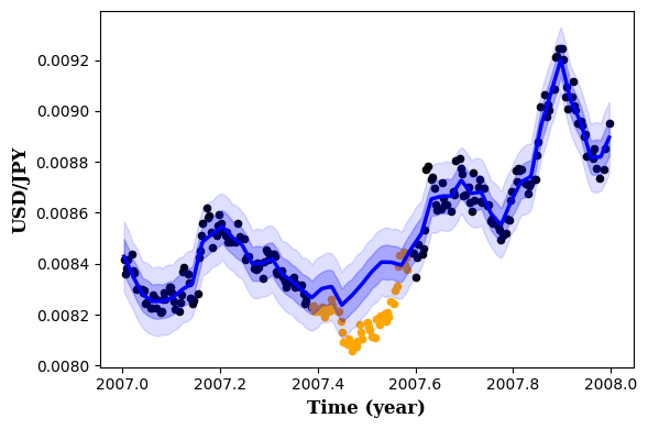
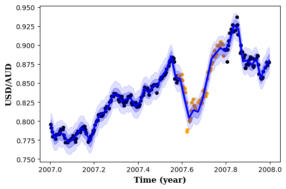
Exchange Rates prediction
This dataset includes daily exchange rates against the USD for ten currencies and three precious metals for the year 2007. Our task is to predict the exchange rates of CAD, JPY, and AUD on specific days, given that all other currencies are observed throughout the year. We follow the same setup as (Álvarez et al., 2010). For GS-LVMOGP models, we use a Matérn-1/2 kernel, consistent with (Bruinsma et al., 2020). Though in this experiment the number of outputs is rather small, and no approximation is required, we included it as a way to show that the mini-batch approach leads to results on par with other small-scale models, as shown in Table 1. Notice that by setting , we obtain a scalable version of the LV-MOGP proposed by Dai et al. (2017). Though its performance is slightly behind LV-MOGP, the GS-LVMOGP with outperforms LV-MOGP on both metrics. As increases, the flexibility in constructing the covariance matrix improves, resulting in enhanced model performance. More information is elaborated in Appendix 7.6.1.
| Model | IGP | COGP | CGP | OILMM | LV-MOGP | GS-LVMOGP | ||
|---|---|---|---|---|---|---|---|---|
| SMSE | 0.251 | 0.256 | 0.186 | |||||
| NLPD | -2.471 | -1.851 | -2.416 | -2.703 | ||||
NYC Crime Count modelling
| RMSE | NLPD | ||
| IGP (G) | 1.9370.030 | 2.1070.022 | |
| OILMM (G) | 1.8570.025 | 1.4930.011 | |
| GS-LVMOGP (G) | 2.2010.125 | 1.4980.299 | |
| 1.9080.381 | 1.5250.206 | ||
| 1.9690.103 | 1.5310.352 | ||
| GS-LVMOGP (P) | 1.7910.023 | 1.2880.003 | |
| 1.7910.023 | |||
We analyze crime patterns across New York City (NYC) using daily complaint data from nyc (2015). Accurate modelling of the seasonal trends and spatial dependencies from crime data can improve police resource allocation efficiency (Aglietti et al., 2019). Following Hamelijnck et al. (2021), the dataset includes spatial locations with observations each. Each location is treated as an output, so . We consider three models IGP, OILMM and our GS-LVMOGP, all using the Matérn-3/2 kernel. We consider Gaussian and Poisson likelihoods for this count data. Table 2 shows the results. The performance comparison of GS-LVMOGP with again indicates that higher improves prediction accuracy. Notably, the Poisson likelihood consistently outperforms the Gaussian likelihood, as it is inherently more suited to the characteristics of count data.
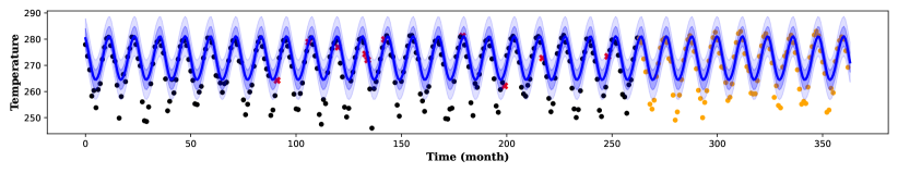
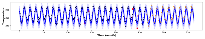
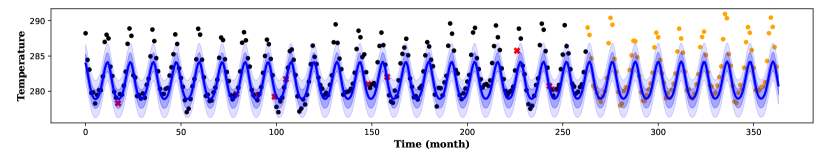
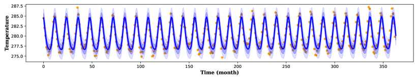
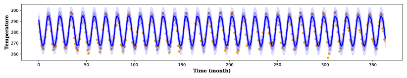
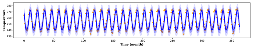
Spatiotemporal Temperature modelling
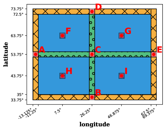
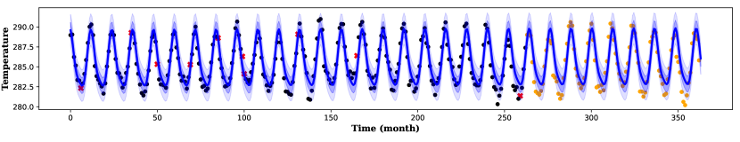
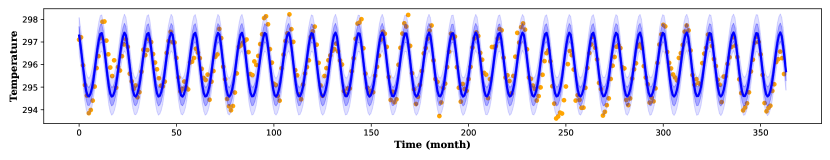
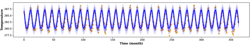
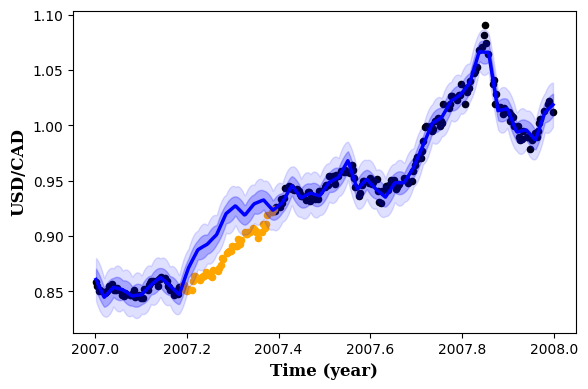
In this section, we address spatiotemporal temperature modelling across Europe, using spatial locations (blue regions in Fig. 1) with months of observations per location. Each spatial location is treated as an output, so , and time is the input. Our tasks include data imputation and extrapolation prediction. For every output, we randomly select data points from the first observations as training data, using the remaining months for imputation testing. The last observations for each output serve as extrapolation test samples. To incorporate spatial information, we set the means of the prior distribution of the latent variables, , to the (longitude, latitude) vector for each output . We compare three models: IGP, OILMM and GS-LVMOGP, all using Matérn–5/2 kernels with a periodic component. Table 4 summarizes the results. From Table 4, with , the GS-LVMOGP outperforms other methods in both imputation and extrapolation tasks. The first plot in Fig. 2 shows predictions for one output in this spatiotemporal dataset. Our model can also extrapolate to unseen locations not included during training, known as output extrapolation, by setting latent variables to the spatial coordinates of chosen locations. The last two plots in Fig. 2 show predictions for two spatial locations excluded during training. Fig. 1 illustrates two types of spatial regions for output extrapolation, marked in green and orange. Locations marked in green are surrounded by training locations (blue), thus the predictions for them are termed as inner output extrapolation, total outputs. In contrast, predictions for the orange regions, referred to as outer output extrapolation, lie on the periphery of the training regions, totalling outputs. The SMSEs for inner and outer output extrapolation are and , respectively. 777The NLPDs for extrapolated outputs are not available as we have no estimates of the parameters .
| IGP | OILMM | GS-LVMOGP | ||||||||||||||
|---|---|---|---|---|---|---|---|---|---|---|---|---|---|---|---|---|
| Imputation | SMSE |
|
|
|
|
|
||||||||||
| NLPD |
|
|
|
|
|
|||||||||||
| Extrapolation | SMSE |
|
|
|
|
|
||||||||||
| NLPD |
|
|
|
|
|
|||||||||||
| MSE | NLPD | ||||||
|---|---|---|---|---|---|---|---|
| GS-LVMOGP |
|
|
|||||
|
|
||||||
|
|
||||||
| OILMM |
|
|
|||||
Climate forecast
We consider the United States Historical Climatology Network (USHCN) daily data set, and we follow a similar setting to De Brouwer et al. (2019), choosing a subset of stations and examining a four-year observational period from 1996 to 2000. The dataset is subsampled as De Brouwer et al. (2019), resulting in an average observations during the first three years for each output. We discard outputs with fewer than three observations and finally have outputs. More details are in Appendix 7.6.4. Our task is to forecast the subsequent three observations following the initial three years of data collection. We use the Matérn-3/2 kernel for GS-LVMOGP and OILMM. Table 4 compares the performance results of our models against OILMM, showing improved performance.
Spatial Transcriptomics
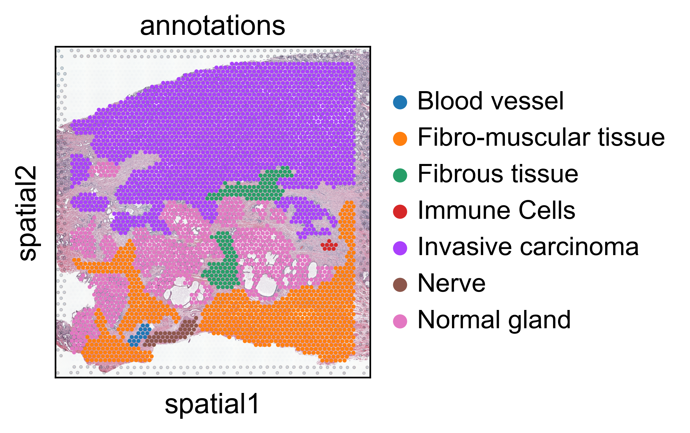
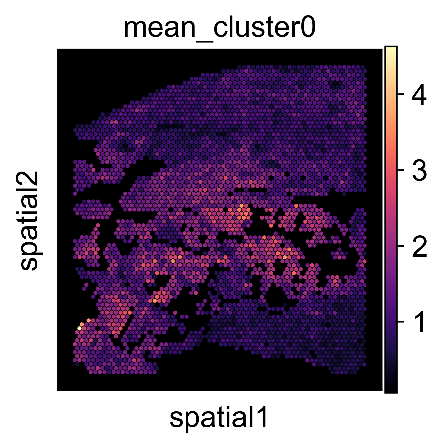
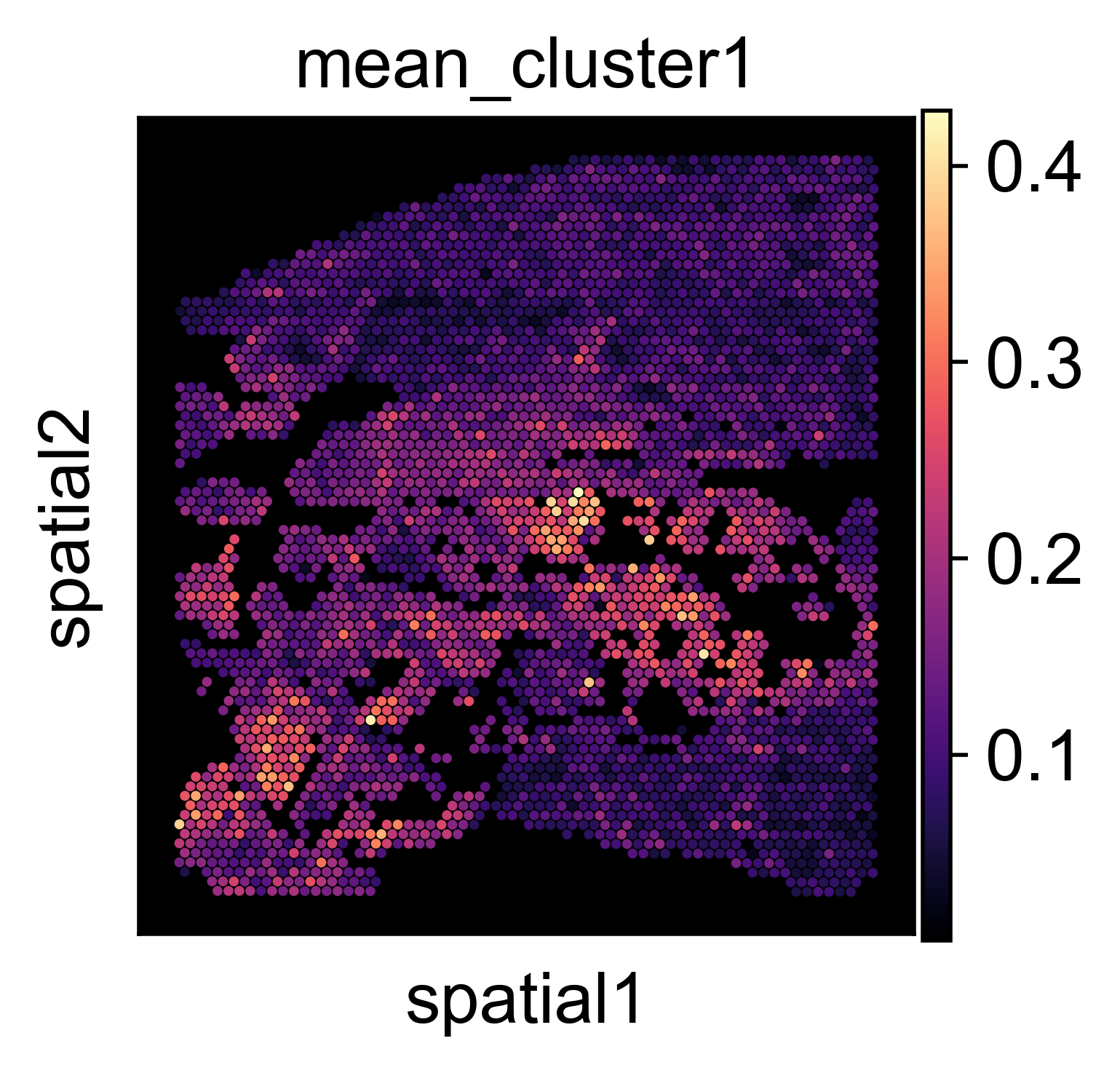
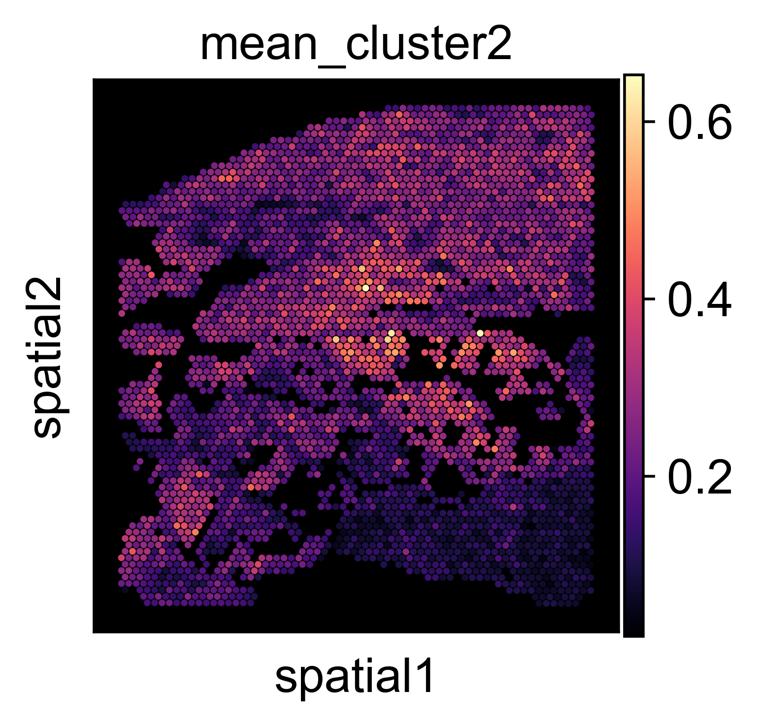
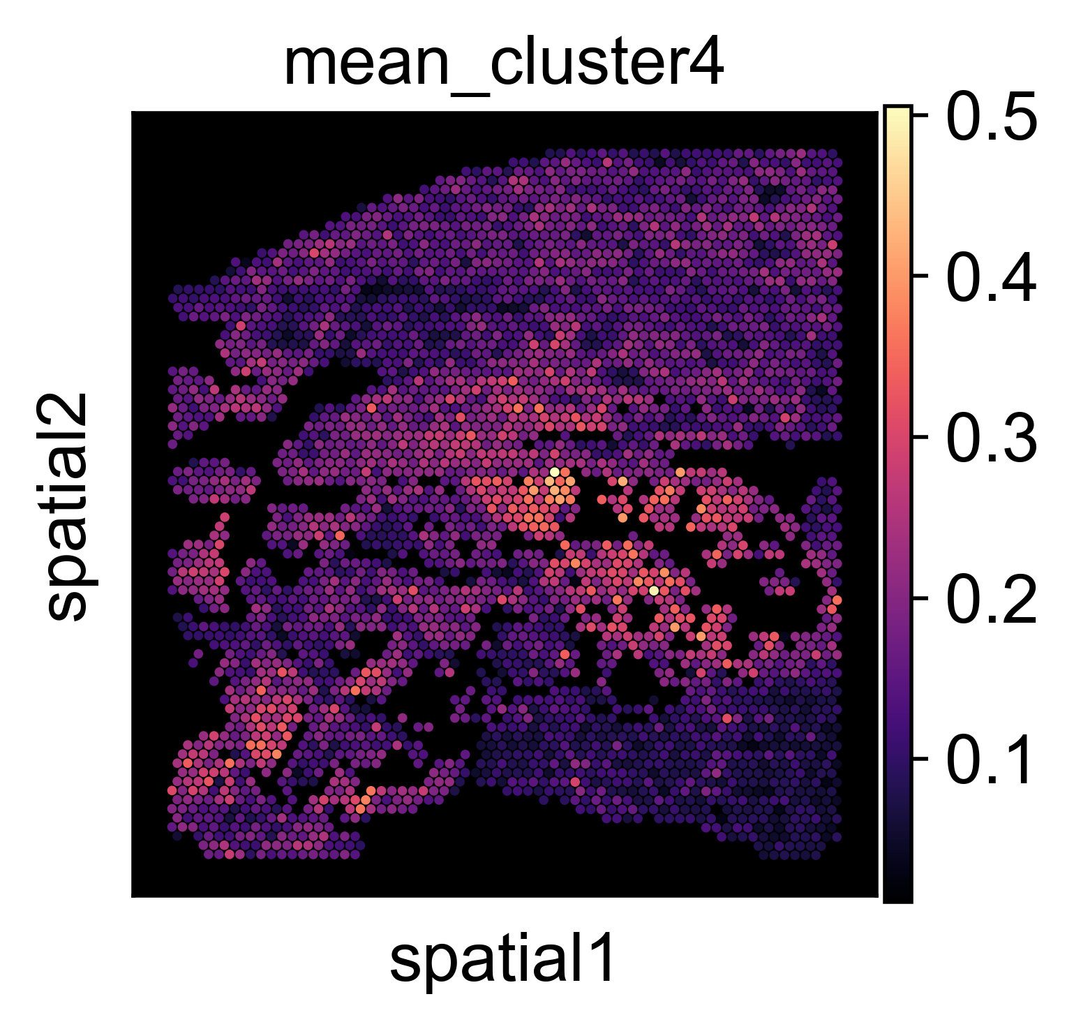
Spatial transcriptomics (Ståhl et al., 2016) offers high-resolution profiling of gene expression while retaining the spatial information of the tissue. Applying machine learning techniques to spatial transcriptomics datasets is vital for understanding the tissue and the disease architecture, potentially enhancing diagnosis and treatment. We consider a 10x Genomics Visium human prostate cancer dataset (10x, ) which contains gene expression counts data from genes measured across spatial locations. Pathologist’s histological annotations for this specific tissue Fig. 3(a) are provided by 10x Genomics. For our model, we use the top highly variable genes calculated using Scanpy’s highly variable genes function (Wolf et al., 2018). Each gene is treated as a different output and the spatial coordinates of cells are regarded as the inputs. We focus on GS-LVMOGP with , using the SE-ARD kernel and Poisson likelihood, and we aim to explore the structure of the latent space with for the genes.
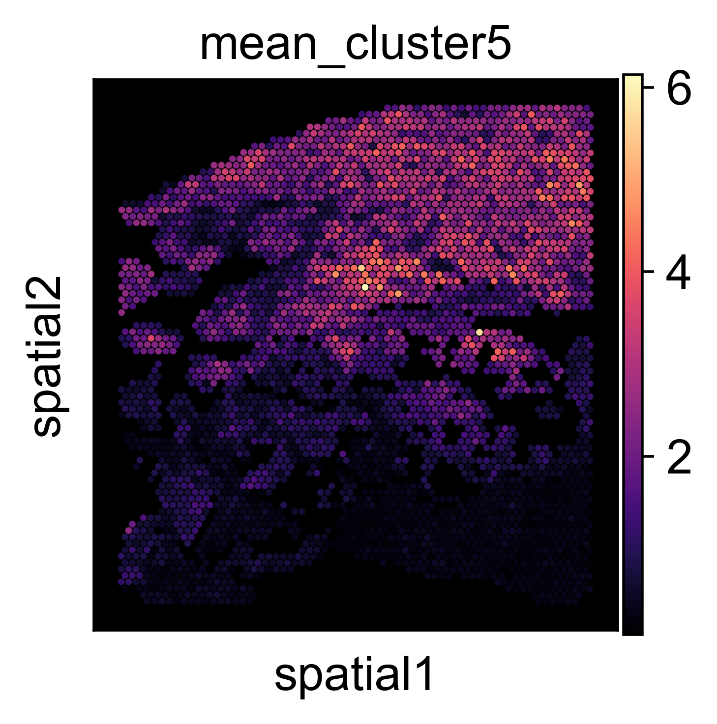
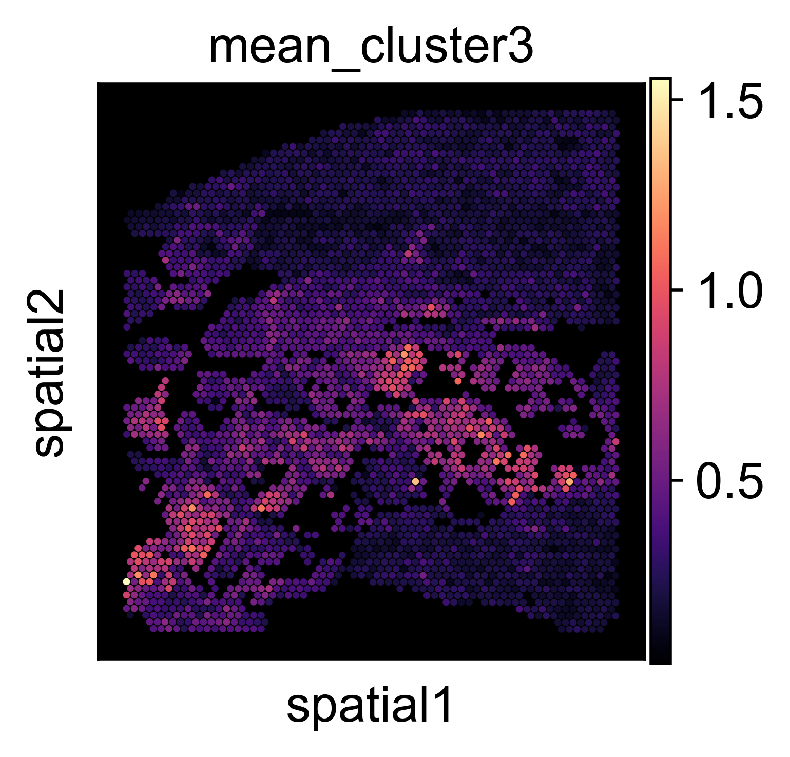
After fitting our model to this dataset, we collect the latent variables for the genes and cluster them into groups using k-means. To plot the spatial distribution of each cluster onto the tissue, we calculate the average expression of the genes in each of the clusters and compare them against the pathologist’s annotated regions. In Fig. 3 we show two of the clusters with genes delineating the tumour (3(b)) and the normal tissue (3(c)) areas, showing good correspondence with the pathologist’s labels (Invasive carcinoma and Normal glands).
Unlike standard clustering practices which solely rely on gene expression to cluster the spatial transcriptomics data, our clustering approach incorporates spatial correlations into the gene clusters. In this way, we can discover distinct spatial tissue regions which might be missed when only considering gene expression.
6 Conclusions
In this paper, we propose GS-LVMOGP, a generalized latent variable multi-output Gaussian process model within a stochastic variational inference framework. By conducting variational inference for latent variables and inducing values , our approach can effectively manage large-scale datasets with both Gaussian and non-Gaussian likelihoods. One feature of the model is that the parameters in the mean vectors and variances for also increase with the number of outputs. Future research could explore imposing structured constraints in the latent space to further reduce the number of parameters required for estimation.
Acknowledgements
MAA has been financed by the EPSRC Research Project EP/V029045/1 and the Wellcome Trust project 217068/Z/19/Z. The authors sincerely thank Xinxing Shi for the insightful and enjoyable discussions throughout the progress of this work. We also appreciate Chunchao Ma for the valuable discussions at the inception of this project. Additionally, we thank Wessel P. Bruinsma for his kind and prompt responses to our queries regarding the datasets.
References
- Williams and Rasmussen [2006] Christopher KI Williams and Carl Edward Rasmussen. Gaussian processes for machine learning, volume 2. MIT press Cambridge, MA, 2006.
- Alvarez et al. [2012] Mauricio A Alvarez, Lorenzo Rosasco, Neil D Lawrence, et al. Kernels for vector-valued functions: A review. Foundations and Trends® in Machine Learning, 4(3):195–266, 2012.
- Wackernagel [2003] Hans Wackernagel. Multivariate geostatistics: an introduction with applications. Springer Science & Business Media, 2003.
- Moreno-Muñoz et al. [2018] Pablo Moreno-Muñoz, Antonio Artés, and Mauricio Alvarez. Heterogeneous multi-output gaussian process prediction. Advances in Neural Information Processing Systems, 31, 2018.
- Yousefi et al. [2019] Fariba Yousefi, Michael T Smith, and Mauricio Alvarez. Multi-task learning for aggregated data using gaussian processes. Advances in Neural Information Processing Systems, 32, 2019.
- Ma et al. [2023] Chunchao Ma, Arthur Leroy, and Mauricio Alvarez. Latent variable multi-output gaussian processes for hierarchical datasets. arXiv preprint arXiv:2308.16822, 2023.
- Journel and Huijbregts [1976] Andre G Journel and Charles J Huijbregts. Mining geostatistics. 1976.
- Higdon [2002] Dave Higdon. Space and space-time modeling using process convolutions. In Quantitative methods for current environmental issues, pages 37–56. Springer, 2002.
- Dai et al. [2017] Zhenwen Dai, Mauricio Álvarez, and Neil Lawrence. Efficient modeling of latent information in supervised learning using gaussian processes. Advances in Neural Information Processing Systems, 30, 2017.
- Bonilla et al. [2007] Edwin V Bonilla, Kian Chai, and Christopher Williams. Multi-task gaussian process prediction. Advances in neural information processing systems, 20, 2007.
- Nguyen et al. [2014] Trung V Nguyen, Edwin V Bonilla, et al. Collaborative multi-output gaussian processes. In UAI, pages 643–652, 2014.
- Lalchand et al. [2022] Vidhi Lalchand, Aditya Ravuri, and Neil D Lawrence. Generalised gaussian process latent variable models (gplvm) with stochastic variational inference. arXiv preprint arXiv:2202.12979, 2022.
- Hoffman et al. [2013] Matthew D Hoffman, David M Blei, Chong Wang, and John Paisley. Stochastic variational inference. Journal of Machine Learning Research, 2013.
- Hensman et al. [2013] James Hensman, Nicolo Fusi, and Neil D Lawrence. Gaussian processes for big data. arXiv preprint arXiv:1309.6835, 2013.
- Alvarez and Lawrence [2011] Mauricio A Alvarez and Neil D Lawrence. Computationally efficient convolved multiple output gaussian processes. The Journal of Machine Learning Research, 12:1459–1500, 2011.
- Titsias and Lawrence [2010] Michalis Titsias and Neil D Lawrence. Bayesian gaussian process latent variable model. In Proceedings of the thirteenth International Conference on Artificial Intelligence and Statistics, pages 844–851. JMLR Workshop and Conference Proceedings, 2010.
- Titsias [2009] Michalis Titsias. Variational learning of inducing variables in sparse gaussian processes. In Artificial Intelligence and Statistics, pages 567–574. PMLR, 2009.
- Kingma and Welling [2013] Diederik P Kingma and Max Welling. Auto-encoding variational bayes. arXiv preprint arXiv:1312.6114, 2013.
- Liu and Pierce [1994] Qing Liu and Donald A Pierce. A note on gauss—hermite quadrature. Biometrika, 81(3):624–629, 1994.
- Ramchandran et al. [2021] Siddharth Ramchandran, Miika Koskinen, and Harri Lähdesmäki. Latent gaussian process with composite likelihoods and numerical quadrature. In International Conference on Artificial Intelligence and Statistics, pages 3718–3726. PMLR, 2021.
- Titsias and Lázaro-Gredilla [2014] Michalis Titsias and Miguel Lázaro-Gredilla. Doubly stochastic variational bayes for non-conjugate inference. In International Conference on Machine Learning, pages 1971–1979. PMLR, 2014.
- Salimbeni and Deisenroth [2017] Hugh Salimbeni and Marc Deisenroth. Doubly stochastic variational inference for deep gaussian processes. Advances in Neural Information Processing Systems, 30, 2017.
- Quinonero-Candela and Rasmussen [2005] Joaquin Quinonero-Candela and Carl Edward Rasmussen. A unifying view of sparse approximate gaussian process regression. The Journal of Machine Learning Research, 6:1939–1959, 2005.
- Liu et al. [2020] Haitao Liu, Yew-Soon Ong, Xiaobo Shen, and Jianfei Cai. When gaussian process meets big data: A review of scalable gps. IEEE Transactions on Neural Networks and Learning Systems, 31(11):4405–4423, 2020.
- Salimbeni et al. [2018] Hugh Salimbeni, Ching-An Cheng, Byron Boots, and Marc Deisenroth. Orthogonally decoupled variational gaussian processes. Advances in Neural Information Processing Systems, 31, 2018.
- Tran et al. [2021] Gia-Lac Tran, Dimitrios Milios, Pietro Michiardi, and Maurizio Filippone. Sparse within sparse gaussian processes using neighbor information. In International Conference on Machine Learning, pages 10369–10378. PMLR, 2021.
- Wu et al. [2022] Luhuan Wu, Geoff Pleiss, and John P Cunningham. Variational nearest neighbor gaussian process. In International Conference on Machine Learning, pages 24114–24130. PMLR, 2022.
- Bartels et al. [2023] Simon Bartels, Kristoffer Stensbo-Smidt, Pablo Moreno-Muñoz, Wouter Boomsma, Jes Frellsen, and Soren Hauberg. Adaptive cholesky gaussian processes. In International Conference on Artificial Intelligence and Statistics, pages 408–452. PMLR, 2023.
- Álvarez et al. [2010] Mauricio Álvarez, David Luengo, Michalis Titsias, and Neil D Lawrence. Efficient multioutput gaussian processes through variational inducing kernels. In Proceedings of the Thirteenth International Conference on Artificial Intelligence and Statistics, pages 25–32. JMLR Workshop and Conference Proceedings, 2010.
- Bruinsma et al. [2020] Wessel Bruinsma, Eric Perim, William Tebbutt, Scott Hosking, Arno Solin, and Richard Turner. Scalable exact inference in multi-output gaussian processes. In International Conference on Machine Learning, pages 1190–1201. PMLR, 2020.
- Alvarez and Lawrence [2008] Mauricio Alvarez and Neil Lawrence. Sparse convolved gaussian processes for multi-output regression. Advances in Neural Information Processing Systems, 21, 2008.
- nyc [2015] 2014–2015 crimes reported in all 5 boroughs of new york city. https://www.kaggle.com/adamschroeder/crimes-new-york-city, 2015. Accessed: 2024-05-19.
- Aglietti et al. [2019] Virginia Aglietti, Theodoros Damoulas, and Edwin V Bonilla. Efficient inference in multi-task cox process models. In The 22nd International Conference on Artificial Intelligence and Statistics, pages 537–546. PMLR, 2019.
- Hamelijnck et al. [2021] Oliver Hamelijnck, William Wilkinson, Niki Loppi, Arno Solin, and Theodoros Damoulas. Spatio-temporal variational gaussian processes. Advances in Neural Information Processing Systems, 34:23621–23633, 2021.
- De Brouwer et al. [2019] Edward De Brouwer, Jaak Simm, Adam Arany, and Yves Moreau. Gru-ode-bayes: Continuous modeling of sporadically-observed time series. Advances in Neural Information Processing Systems, 32, 2019.
- Ståhl et al. [2016] Patrik L Ståhl, Fredrik Salmén, Sanja Vickovic, Anna Lundmark, José Fernández Navarro, Jens Magnusson, Stefania Giacomello, Michaela Asp, Jakub O Westholm, Mikael Huss, et al. Visualization and analysis of gene expression in tissue sections by spatial transcriptomics. Science, 353(6294):78–82, 2016.
- [37] X Genomics. https://www.10xgenomics.com/resources/datasets/human-prostate-cancer-adenocarcinoma-with-invasive-carcinoma-ffpe-1-standard-1-3-0.
- Wolf et al. [2018] F Alexander Wolf, Philipp Angerer, and Fabian J Theis. Scanpy: large-scale single-cell gene expression data analysis. Genome biology, 19(1):1–5, 2018.
- Kingma and Ba [2014] Diederik P Kingma and Jimmy Ba. Adam: A method for stochastic optimization. arXiv preprint arXiv:1412.6980, 2014.
- Menne et al. [2015] MJ Menne, CN Williams Jr, and RS Vose. Long-term daily climate records from stations across the contiguous united states, 2015.
7 Appendix
7.1 ELBO deviation for LV-MOGP
In this section, we describe in more detail the deviation of the evidence lower bound for LV-MOGP.
| (21) | ||||
Now we focus on the term. Notice that
| (22) | ||||
and,
| (23) | ||||
then, we have:
| (24) | ||||
where , and . Notice that if there are no missing values, Eq. (24) can be further simplified by exploiting properties of the Kronecker product, resulting in equation (8) in Dai et al. [2017]. But in the general case (with missing values), we use Eq. (24) to compute for each output , and .
7.1.1 Computation of statistics , and
The statistics and can be simplified by exploiting the Kronecker product structure.
| (25) | ||||
The statistics of , and can be approximated by Monte Carlo methods. For some particular kernels, they can be analytically solved. For instance, for the SE-ARD kernel. Recall , with being diagonal matrix, denotes the elements on the diagonal. th component of is denoted as . We are willing to derive analytical formulae for , notice that if .
Recall for SE-ARD kernel, for any :
| (26) |
where and is the th component of . The term is trivially computed as .
Consider latent inducing variables , we have:
| (27) | ||||
Notice the second line uses the conclusion of the product of Gaussians, which is:
| (28) |
where , and , .
7.2 Parametrization technique of in GS-LVMOGP
When , employing the parameterization , as detailed in Section 3.2, results in covariance matrix of also exhibiting a Kronecker product structure. This is because:
| (30) |
thus, and,
| (31) | ||||
For , the Cholesky factor can not be factorized in general, so the covariance matrix of does not have Kronecker product structure.
Another advantage of the proposed parametrization technique is that we have more efficient computation of the term in the ELBO. Firstly, notice
| (32) |
for two general Gaussian distributions and , computation of is based on the following formula, with complexity:
| (33) |
while the KL divergence between a Kronecker product structured Gaussian distribution and a standard Gaussian distribution, the can be largely simplified, with only complexity :
| (34) | ||||
7.3 Gauss-Hermite quadrature
Gauss-Hermite quadrature is a numerical technique specifically designed for computing integrals of functions that have a Gaussian (or exponential) weight function. This method is particularly useful when dealing with integrals where the integrand involves a Gaussian-weighted function, making it an ideal choice for expectations involving Gaussian distributions in probabilistic modelling, and in particular, Gaussian process models.
In Gauss-Hermite, the weight function is , the integral it approximates has form . The approximation is given by:
| (35) |
where are the roots of the n-th Hermite polynomial, , and are the corresponding weights, calculated as: .
7.3.1 Numerical integration
Recall are Gaussian distribution denoted as , where
| (36) | ||||
To apply Gaussian-Hermite quadrature, we first re-write the integration by change of variables:
| (37) | ||||
This transforms the integral to
Now we apply Gauss-Hermite quadrature,
| (38) |
7.3.2 Practical Steps
-
•
Determine the degree : the choice of balances between computational cost and accuracy. In our experiments, we use .
-
•
Find and : typically be looked up in numerical libraries or computed using software that handles numerical analysis.
-
•
Evaluate : Compute this term at for each .
-
•
Compute the weighted sum, which is the approximation of the integral.
7.4 Discussion about ICM, LMC, LV-MOGP and GS-LVMOGP
The LV-MOGP model is akin to the Intrinsic Coregionalization Model (ICM) in that it utilizes a single coregionalization matrix. In contrast, the GS-LVMOGP model is more similar to the Linear Model of Coregionalization (LMC), as it allows for the possibility of multiple coregionalization matrices (). Table 5 provides a comparative comparison of these methods.
| Models | Approach | # Parameters | # Coreg. Matrices | SVI | Likelihood | ||
|---|---|---|---|---|---|---|---|
| ICM | |||||||
| LMC | |||||||
| LV-MOGP |
|
Gaussian | |||||
| GS-LVMOGP |
|
Any |
7.5 Integration of latent variables for prediction
The prediction problem for given output and input involves an integration w.r.t uncertain latent variables , as shown in Eq. (20). This integration is in general intractable, and recall in Section 3.4, we adopt an approach to use means of to approximate the integral. In this section, we provide an alternative approach: a Gaussian approximation (compute first and second moment) for the predictive distribution.
| (39) | ||||
we denote the mean and variance for as and , where
| (40) | ||||
We consider the first and second moment for , which we denote as and respectively.
| (41) | ||||
| (42) | ||||
there are three terms to compute: , and ,
| (43) | ||||
| (44) | ||||
| (45) | ||||
integration over appears in three terms: , and . These terms can be further simplified by Kronecker product decomposition: first, consider:
| (46) | ||||
and,
| (47) | ||||
then consider:
| (48) | ||||
where
| (49) |
Therefore, the key to compute and relies on the computation of following statistics:
| (50) |
| (51) |
| (52) |
The computation of the above three statistics are the same as in Appendix 7.1.1.
7.6 Experiment Settings
We use the following metrics in the experiments: MSE (mean square error), RMSE (root mean square error), SMSE (standardised mean square error), and NLPD (negative log predictive density). denotes prediction value and refers to the ground truth:
| (53) |
| (54) |
| (55) |
| (56) |
With a Gaussian likelihood, we make use of closed-form solutions to the NLPD, otherwise we approximate it using Gaussian Hermite quadrature.
Some hyperparameters used in experiments are shown in Table 6.
| Optimizer | Mini-batch size | Iterations | lr | |||||
|---|---|---|---|---|---|---|---|---|
| Exchange | 20 | 50 | 3 | 3 | Adam | 500 | 5000 | 0.01 |
| USHCN | 10 | 50 | 2 | 1 | Adam | 500 | 10000 | 0.1 |
| Spatio-Temporal | 10 | 20 | 2 | 1 | Adam | 500 | 5000 | 0.1 |
| NYC Crime Count | 20 | 50 | 2 | 1 | Adam | 1000 | 5000 | 0.1 |
| Spatial Transcriptomics | 50 | 50 | 3 | 1 | Adam | 1000 | 200000 | 0.1 |
The experiments are run on a MacBook Pro with M3 Max and 36G RAM. Except for spatial transcriptomics experiments, all experiments (for each run) are finished in 30 minutes. The spatial transcriptomics experiments take around 8 hours on the laptop.
7.6.1 More experiment details on exchange dataset
The ten international currencies are: CAD, EUR, JPY, GBP, CHF, AUD, HKD, NZD, KRW, MXN, and the three precious metals are gold, silver, and platinum. We make plots for the outputs corresponding to CAD, JPY and AUD. We also report the error bars for GS-LVMOGP on the exchange dataset, shown in Table 7. We take the exchange dataset as an example to experiment with the relationship between the computational time consumption and mini-batch size .
| GS-LVMOGP | |||
|---|---|---|---|
| Q=1 | Q=2 | Q=3 | |
| SMSE | 0.2560.1 | 0.1860.019 | 0.1670.019 |
| NLPD | -1.8510.9 | -2.4160.24 | -2.7030.19 |
7.6.2 More experiments details on spatiotemporal dataset
The dataset can be downloaded from https://cds.climate.copernicus.eu/cdsapp#!/dataset/projections-cmip5-monthly-single-levels?tab=form, and we only consider spatial region plotted in Fig. 1, that is longitude from W to E, latitude from N to N. The temperature is measured by the Kelvin unit.
For the OILMM [Bruinsma et al., 2020] method, there is a hyper-parameter , that determines the number of latent processes in the model. We tried a different setting of from 1 to 100, with preliminary experiment results shown in Table 8, and then we choose to report results on the main table in Table 4. In the paper, we reported the SMSE metric for extrapolated outputs with no training data. The computation of SMSE for them is no longer standardised w.r.t. mean of but mean of .
| imputation | SMSE | 0.276 | 0.252 | 0.134 | 0.130 | 0.788 | 1.0 |
|---|---|---|---|---|---|---|---|
| NLPD | 2.943 | 2.944 | 2.819 | 36.609 | 19.202 | 12.357 | |
| extrapolation | SMSE | 0.285 | 0.258 | 0.155 | 0.202 | 0.798 | 1.0 |
| NLPD | 3.045 | 3.049 | 3.063 | 11.022 | 17.778 | 13.127 |
7.6.3 More experiment details on NYC Crime
Similar to the spatiotemporal dataset, we do preliminary experiments for OILMM with different numbers of latent processes on the NYC Crime dataset. The results are shown in Table 9, and we again choose for main experiments in Table 2 in the paper.
| RMSE | 1.856 | 1.857 | 1.857 | 1.858 | 1.858 | 1.865 |
| NLPD | 1.545 | 1.493 | 1.493 | 1.493 | 1.500 | 1.510 |
Similar to spatiotemporal experiments, we can also encode spatial information into the prior distribution of the latent variables . We run an experiment with this setting and compare it against methods in [Hamelijnck et al., 2021], shown in Table 10.
| RMSE | NLPD | ||
| (P) | 2.770.06 | 1.660.02 | |
| (P) | 2.750.04 | 1.630.02 | |
| (P) | 3.200.14 | 1.820.05 | |
| (P) | 3.020.18 | 1.760.05 | |
| GS-LVMOGP (G) | 2.1570.062 | 1.5000.329 | |
| 2.0860.063 | 1.3570.132 | ||
| 2.0750.048 | 1.3630.187 | ||
| GS-LVMOGP (P) | 1.7910.023 | 1.2870.003 | |
| 1.7910.023 | 1.2870.003 | ||
| 1.7900.024 | 1.2870.003 | ||
7.6.4 USHCN-Daily: more details
The United States Historical Climatology Network (USHCN) data set as detailed by Menne et al. [2015], includes records of five climate variables across a span of over years at meteorological stations throughout the United States. It is publicly available and can be downloaded at the following address: https://cdiac.ess-dive.lbl.gov/ftp/ushcn_daily/. All state files contain daily measurements for variables: precipitation, snowfall, snow depth, minimum temperature, and maximum temperature.
We follow the same data pre-processing procedure as in De Brouwer et al. [2019], and processed data is kindly provided in https://github.com/edebrouwer/gru_ode_bayes. We further filter out outputs with or less training observations. The final dataset in the experiment has outputs and training data points.
7.6.5 More experiment details
Similar to the spatiotemporal and NYC Crime datasets, we also do preliminary experiments for OILMM with different numbers of latent processes on the USHCN dataset. Based on the results shown in Table 12, we again choose for main experiments in Table 4.
| MSE | 0.894 | 0.894 | 0.893 | 0.894 | 0.894 | 0.894 |
| NLPD | 811.39 | 810.82 | 810.83 | 811.37 | 816.45 | 822.73 |
7.6.6 More details about spatial transcriptomics experiment
In Fig. (7) we show the mean gene expression of the remaining clusters, where, similarly to cluster (3(c)), clusters (7(a)) and (7(b)) align with the normal tissue area. Cluster (7(c)) and cluster (7(d)) contain a combination of normal and tumour regions. It is good to note here that the highly variable genes used in the model are mainly expressed in the normal area of the tissue which makes that area more prevalent in the clusters. In future applications, a larger gene sample with genes that are enriched to other areas of the tissue would better represent the heterogeneity it and therefore the clusters will be better resolved.
7.7 Limitations
In this work, the computational complexity is carefully reduced for by decompositing matrix inversion. However, the computational complexity for has not been well addressed, where a naive matrix inversion complexity is applied. In future work, it is important to investigate and develop efficient algorithms for matrix inversion when to further optimize computational performance. Additionally, exploring alternative mathematical techniques or approximations that can maintain accuracy while reducing complexity will be crucial for advancing this area of research.
7.8 Broader impacts
This research addresses issues in climate modelling and human spatial transcriptomic, with potential benefits for society. By enhancing the accuracy of climate model prediction, our work contributes to a deeper understanding of environmental dynamics. This, in turn, can aid in more effective planning and production, while also providing insights into climate change that are crucial for mitigation strategies. Our study includes a spatial transcriptomics dataset on human prostate cancer. This dataset is invaluable for advancing the understanding of disease progression and treatment, thereby offering potential improvements in healthcare and patient outcomes. We have not identified any aspects of this research that pose harm to human society.