A robust theory of thermal activation in magnetic systems with Gilbert damping

Abstract

Magnetic systems can exhibit thermally activated transitions whose timescales are often described by an Arrhenius law. However, robust predictions of such timescales are only available for certain cases. Inspired by the harmonic theory of Langer, we derive a general activation rate for multi-dimensional spin systems. Assuming local thermal equilibrium in the initial minimum and deriving an expression for the flow of probability density along the real unstable dynamical mode at the saddle point, we obtain the expression for the activation rate that is a function of the Gilbert damping parameter, $\alpha$. We find that this expression remains valid for the physically relevant regime of $\alpha\ll 1$. When the activation is characterized by a coherent reorientation of all spins, we gain insight into the prefactor of the Arrhenius law by writing it in terms of spin wave frequencies and, for the case of a finite antiferromagnetic spin chain, obtain an expression that depends exponentially on the square of the system size indicating a break-down of the Meyer-Neldel rule.

I Introduction

At low temperature, finite-size systems can be arrested dynamically over long time and only rarely undergo thermally activated transitions. Predicting the fluctuation timescale for nanoscale magnetic systems was first addressed by Néel, who derived a typical Arrhenius activation law for the time a ferromagnetic nanoparticle takes to reorient its magnetization [1]. In general, this Arrhenius behaviour is retrieved for any finite size transition and tells us that the inverse activation time, i.e. the activation rate $\Gamma$, decreases exponentially with the energy difference between the initial state and the state with the maximal energy during the transition, i.e. the energy barrier $\Delta E$, giving $\Gamma\propto e^{-\Delta E/K_{B}T}$.

In contemporary problems with multiple degrees of freedom, such states correspond to a local minimum and a saddle point of a high-dimensional energy landscape. While the local minimum is a priori known due to its statistical relevance as a stable state, the saddle point can be difficult to identify. There exists however in silico methods based on the iterative exploration of the energy landscape that can locate nearby saddle points. Among many, the Nudged Elastic Band (NEB) method [2], the dimer method [3, 4, 5] and the Activation-Relaxation Technique (ART) [6, 7, 8, 9] are the most documented in the literature. Although all of them have been initially developed for Newtonian systems, NEB and ART have also been implemented for finite-size magnetic systems [10, 11, 12]. The present authors have made available a general implementation of a magnetic variant of ART (mART [13]) applying it to not only finite systems but also to uncovering localized magnetic excitations in bulk phases and relaxation processes in spin glasses [14].

Although the energy barrier dependence of the activation rate is well-known, a complete prediction, of the form $\Gamma=\nu e^{-\Delta E/K_{B}T}$, requires more considerations. In particular, the dynamics needs to be specified to compute the prefactor $\nu$. In the context of classical magnetism, where the dynamics is defined by the Landau-Lifschitz (LL) equation, a prediction of the prefactor was first obtained by Brown for a single magnetic moment with a uniaxial anisotropy [15, 16]. The derivation was essentially adapted from Kramers, who found the solution for a Brownian particle by solving the relevant Fokker-Planck equation [17]. For general magnetic systems with multiple degrees of freedom, several approaches can be found in the literature [18, 19, 20, 21, 22, 23, 24, 25, 26, 27, 28], while some experimental problem remains unsolved [29, 30]. Although the general method of Langer [18, 31] and the spin method of Bessarab et al. [23] result in a similar prefactor depending on the product of the modes of the second derivative of the energy (the Hessian), which can be interpreted as an entropic contribution [25, 26], the latter does not account for thermal fluctuations making the solution independent of the Gilbert damping parameter $\alpha$. In contrast, the method of Langer, which relies explicitly on reaching equilibrium in the minimum basin before the activation, is consistent with the fluctuation-dissipation theorem. Nevertheless, due to the equilibrium assumption being incompatible with an almost-deterministic precessional dynamics at small $\alpha$, the result of Langer is believed to be only valid for $\alpha\gtrsim 1$ and thus not applicable to most materials which have values of $\alpha$ well below unity [32, 16]

In this paper, we apply the general method of Langer to spin systems and demonstrate that its range of application can be extended to the $\alpha\ll 1$ regime of damping. We will achieve this by evaluating the time to reach equilibrium in a minimum basin and comparing it to the activation time to produce a validation condition highlighting the robustness of the theory for $\alpha\ll 1$, when the energy barrier is larger than the thermal energy. In addition, we will show that the result of Langer can be simply obtained by imposing the probability density to flow along the only real unstable dynamical mode at the saddle point. Once the framework and the relevance of the theory for spin systems are shown, we will gain insight into the resulting Arrhenius law for coherent transitions, i.e. when the order is sustained during the activation, giving explicitly the dependence in $\alpha$ and a formulation of the prefactor of the Arrhenius law in terms of spin wave frequencies. With the example of an antiferromagnetic spin chain, we will obtain an explicit expression of the prefactor, highlighting its dependence on the system size.

Spin systems require us, in principle, to deal with the curved spin space when the spin magnitude is fixed. This difficulty can be circumvented for the harmonic theory of Langer by working in the Euclidean tangent bundle made of the tangent spaces, i.e. the transverse space to the spin configurations. After describing the relevant stochastic LL dynamics in Sec. II.1, we define these spaces and start by describing equilibrium in a minimum basin, i.e. deriving the partition function by expanding the Hamiltonian and the dynamics from the minimum in the appropriate tangent space in Sec. II.2. In Sec. II.3, we account for the existence of a saddle point and evaluate the probability density flux consistently with an initial equilibrium at the minimum. In Sec. II.4, the activation rate is evaluated by integrating the probability density flux across the saddle point. In Sec. II.5, we determine the condition for the system to achieve equilibrium in the minimum before the activation in order to validate the theory. For systems that have a lattice translational invariance and exhibit a coherent activation, we rewrite the prefactor of the Arrhenius law in Sec. II.6 as a function of Fourier modes of the Hessian and spin wave frequencies when $\alpha\ll 1$. For the coherent activation of an antiferromagnetic chain, we derive an analytical expression for the prefactor in terms of system size and parameters in Sec. III. The method and its application are discussed in Sec. IV.

II Method

II.1 Stochastic Landau-Lifschitz dynamics

The temporal evolution of a spin system at finite temperature can be described phenomenologically by the following stochastic LL equation [33, 34]:

$$\partial_{t}\bm{s}_{i}=-\gamma\bm{s}_{i}\times\left(\bm{h}_{i}+\bm{b}_{i}\right)-\frac{\alpha\gamma}{S}\bm{s}_{i}\times\left(\bm{s}_{i}\times\bm{h}_{i}\right)\;.$$ (1)

$\bm{s}_{i}$ is the spin at site $1\leq i\leq N$, $S$ the corresponding magnitude assumed fixed and site independent, $\alpha$ the Gilbert damping parameter and $\gamma$ the gyromagnetic ratio. The effective field $\bm{h}_{i}$ is derived from the underlying spin Hamiltonian $\mathcal{H}$:

$$\bm{h}_{i}=-\frac{\partial\mathcal{H}}{\partial\bm{s}_{i}}\;.$$ (2)

The Gaussian fluctuating field $\bm{b}_{i}$ is defined by $\left<b_{i}^{\alpha}(t)\right>=0$ and

$$\left<b_{i}^{\alpha}(t)b_{j}^{\beta}(t^{\prime})\right>=2\alpha\frac{K_{B}T}{\gamma S}\delta^{\alpha\beta}\delta_{ij}\delta(t-t^{\prime})\;.$$ (3)

This dynamical equation can be made dimensionless through the following transformations:

$$\begin{split}\bm{s}_{i}&\rightarrow S\bm{s}_{i}\\ \mathcal{H}&\rightarrow K_{B}T\mathcal{H}\\ \bm{h}_{i}&\rightarrow\frac{K_{B}T}{S}\bm{h}_{i}\\ t&\rightarrow\frac{S}{\gamma K_{B}T}t\;.\end{split}$$ (4)

We obtain

$$\partial_{t}\bm{s}_{i}=-\bm{s}_{i}\times\left(\bm{h}_{i}+\bm{b}_{i}\right)-\alpha\bm{s}_{i}\times\left(\bm{s}_{i}\times\bm{h}_{i}\right)\;,$$ (5)

with the variance of $\bm{b}_{i}$ that simplifies to $2\alpha$.

II.2 Dynamics and equilibrium in a minimum basin

We initially assume that the system evolves in equilibrium in a local minimum basin. We aim to describe the Hamiltonian and the dynamics to the leading perturbative order from the local minimum and derive the probability density corresponding to equilibrium in the basin.

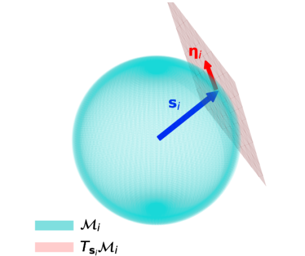
Figure 1: Illustration of the curved phase space $\mathcal{M}_{i}$ of spin $\bm{s}_{i}$ and the tangent space $T_{\bm{s}_{i}}\mathcal{M}$ with a perturbation $\bm{\eta}_{i}$.

Due to the fixed spin magnitude, the phase space $\mathcal{M}_{i}$ of spin $i$ is curved. A perturbation of the spin $\bm{s}_{i}$ can be represented by a transverse vector $\bm{\eta}_{i}$, which belongs to the Euclidean tangent plane $T_{\bm{s}_{i}}\mathcal{M}_{i}=\{\bm{\eta}_{i}|\bm{\eta}_{i}\cdot\bm{s}_{i}=0\}$, as illustrated in Fig. 1. Note that $T_{\bm{s}_{i}}\mathcal{M}_{i}$ is embedded in the Euclidean three-dimensional space in which $\bm{s}_{i}$ can be expressed, which legitimates, for example, the scalar product “$\cdot$” in the definition. By extension, a state $\{\bm{s}_{i}\}$ of the system phase space $\mathcal{M}$ can be perturbed by $\bm{\eta}=\operatorname*{\text{\raisebox{1.07639pt}{\scalebox{0.8}{$\bigotimes$}}}}_{i}\bm{\eta}_{i}$, which lives in the $2N$-dimensional tangent space $T_{\{\bm{s}_{i}\}}\mathcal{M}=\cup_{i}T_{\bm{s}_{i}}\mathcal{M}_{i}$. Thanks to this representation, we can now expand the Hamiltonian at any state by expressing the derivatives in the tangent space. In particular, at the minimum, we consider the harmonic expansion obtained from the Hessian $\mathrm{H}^{(m)}$. Acknowledging the fact that the Hamiltonian is commonly expressed in the 3N-dimensional embedding space, we follow Ref. [14] and write the matrix elements of the Hessian for the minimum given by $\{\bm{s}_{i}\}$ as

$$\left(\mathrm{H}^{(m)}\right)_{ij}^{\beta\gamma}=\sum_{\alpha}\left.\partial_{j}^{\gamma}\mathrm{P}_{i}^{\beta\alpha}\partial_{i}^{\alpha}\mathcal{H}\right|_{\{\bm{s}_{i}\}}\;,$$ (6)

where $\mathrm{P}_{i}$ is the projection operator on the tangent plane $T_{\bm{s}_{i}}\mathcal{M}_{i}$:

$$\mathrm{P}_{i}^{\alpha\beta}=\delta^{\alpha\beta}-s_{i}^{\alpha}s_{i}^{\beta}\;.$$ (7)

The Harmonic expansion is therefore

$$\begin{split}\mathcal{H}^{(m)}&=E^{(m)}+\frac{1}{2}\bm{\eta}^{T}\mathrm{H}^{(m)}\bm{\eta}\\ &=E^{(m)}+\frac{1}{2}\left(\sum_{ij,\alpha\beta}\eta_{j}^{\beta}\eta_{i}^{\alpha}\partial_{j}^{\beta}\partial_{i}^{\alpha}\mathcal{H}-\sum_{i,\alpha\beta}\eta_{i}^{\beta}\eta_{i}^{\beta}s_{i}^{\alpha}\partial_{i}^{\alpha}\mathcal{H}\right)\;,\end{split}$$ (8)

where we explicitly write the Hessian in embedding space using $\bm{\eta}_{i}^{T}\bm{s}_{i}=0$ in the second line to obtain a formulation in terms of regular Euclidean derivatives. Within this harmonic expansion represented in Fig. 2a, the stochastic LL equation (Eq. 5) becomes

$$\partial_{t}\bm{\eta}=-\left(\mathrm{Q}+\alpha\mathrm{I}\right)\mathrm{H}^{(m)}\bm{\eta}+\bm{b}\;,$$ (9)

with $\bm{b}=\operatorname*{\text{\raisebox{1.07639pt}{\scalebox{0.8}{$\bigotimes$}}}}_{i}\bm{b}_{i}$ being now the Gaussian fluctuation field projected onto the tangent space. $\mathrm{I}$ is the identity matrix coming from the isotropic dissipative part of the dynamics and $\mathrm{Q}$ is an orthogonal matrix corresponding to a rotation of every transverse spin component by $\pi/2$ which arises from the precessional dynamics. For any local basis (i.e. where every basis vector can be indexed by a unique site) of the tangent space at the minimum $T_{(m)}\mathcal{M}$, $(\mathrm{Q}+\alpha\mathrm{I})$ is block diagonal with the equivalent blocks:

$$\left(\mathrm{Q}+\alpha\mathrm{I}\right)_{i}=\begin{pmatrix}\alpha&1\\ -1&\alpha\end{pmatrix}\;.$$ (10)

The density $\rho^{(m)}\left(\bm{\eta},t\right)$ corresponding to the temporal evolution in Eq. 9 must fulfill the following Fokker-Planck equation, which takes the form of a continuity equation:

$$\partial_{t}\rho^{(m)}=\nabla\cdot\bm{\Phi}^{(m)}\;,$$ (11)

for the density flux:

$$\bm{\Phi}^{(m)}(\bm{\eta})=\left(\mathrm{Q}+\alpha\mathrm{I}\right)\left(\mathrm{H}^{(m)}\bm{\eta}+\nabla\right)\rho^{(m)}\;.$$ (12)

We consider the equilibrium solution ($\bm{\Phi}^{(m)}=\bm{0}$) by considering the kernel of $\mathrm{H}^{(m)}\bm{\eta}+\nabla$ to obtain:

$$\rho^{(m)}\left(\bm{\eta}\right)=\frac{\exp\left[-\mathcal{H}^{(m)}(\bm{\eta})\right]}{Z^{(m)}}\;,$$ (13)

with $Z^{(m)}$ the partition function normalizing the density. By defining the ordered set of eigenvalues $\{\varepsilon_{n}^{(m)}\}$ of the Hessian, $\mathrm{H}^{(m)}$, with respective eigenvectors $\{\bm{\phi}_{n}\}$, the partition function can be written in the closed-form:

$$\begin{split}Z^{(m)}&=e^{-E^{(m)}}\int\exp\left(-\frac{1}{2}\bm{\eta}^{T}\mathrm{H}^{(m)}\bm{\eta}\right)d\bm{\eta}\\ &=e^{-E^{(m)}}\sqrt{\prod_{n=1}^{2N}\frac{2\pi}{\varepsilon_{n}^{(m)}}}\;.\end{split}$$ (14)

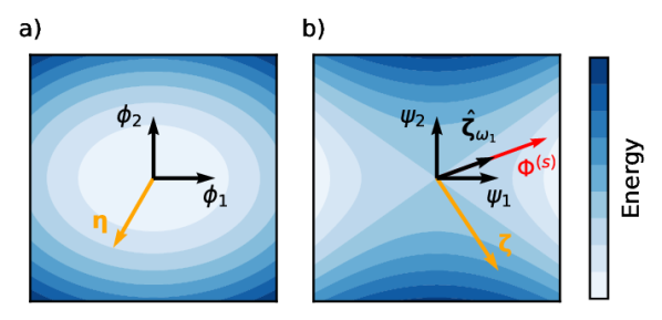
Figure 2: a) Schematic of the harmonic expansion of the energy about the minimum $\mathcal{H}^{(m)}$ and representation of a perturbation $\bm{\eta}$ and the modes $\{\bm{\phi}_{n}\}$ of the Hessian $\mathrm{H}^{(m)}$. b) Similar schematic at the saddle point with the perturbation $\bm{\zeta}$ and the modes $\{\bm{\psi}_{n}\}$ of the Hessian $\mathrm{H}^{(s)}$ as well as the density flux $\bm{\Phi}^{(s)}$, which is aligned with the unique real unstable dynamical mode $\hat{\bm{\zeta}}_{w_{1}}$. The activation rate (Eq. 26) is obtained from the integral over the subspace spanned by $\bm{\psi}_{2}$ of the density flux $\bm{\Phi}^{(s)}$ projected on $\bm{\psi}_{1}$.

II.3 Density flux at the saddle point

We consider now a first-order saddle point surrounding the local minimum. It is characterized by the following Harmonic expansion:

$$\begin{split}\mathcal{H}^{(s)}(\bm{\zeta}&)=E^{(s)}+\frac{1}{2}\bm{\zeta}^{T}\mathrm{H}^{(s)}\bm{\zeta}\\ &=E^{(s)}+\frac{1}{2}\sum_{n=1}^{2N}\varepsilon_{n}^{(s)}\left(\bm{\psi}_{n}^{T}\bm{\zeta}\right)^{2}\;,\end{split}$$ (15)

with $\bm{\zeta}$ a perturbation in the tangent space of the saddle point $T_{(s)}\mathcal{M}$ and the spectrum of the Hessian $\mathrm{H}^{(s)}$: $\{\varepsilon^{(s)}_{n}|\varepsilon^{(s)}_{1}<0,\varepsilon^{(s)}_{m}>0\quad\forall m>1\}$ with respective eigenvectors $\{\bm{\psi}_{n}\}$. These are represented in Fig. 2b. We want to evaluate the density flux at the saddle point $\bm{\Phi}^{(s)}$ to find the activation rate (see Sec. II.4). To evaluate $\bm{\Phi}^{(s)}$, we assume a sufficiently long timescale, such that equilibrium is achieved in the local minimum basin and we verify the consistency of this approach later in Sec. II.5. The first consequence of this assumption is that we can consider thermally-averaged trajectories in the minimum up to the saddle point, which will give us the orientation of the density flux $\bm{\Phi}^{(s)}$. Indeed, the thermally-averaged dynamics, i.e. the deterministic part of Eq. 9, writes at the saddle point:

$$-\left(\mathrm{Q}+\alpha\mathrm{I}\right)\mathrm{H}^{(s)}\bm{\zeta}=\partial_{t}\bm{\zeta}\;.$$ (16)

After a Fourier transform in time ($\bm{\zeta}_{w}=\int\bm{\zeta}e^{iwt}dt$), the dynamical modes become the solution of a right-eigenvector problem for the non-symmetric matrix $\left(\mathrm{Q}+\alpha\mathrm{I}\right)\mathrm{H}^{(s)}$:

$$\left(\mathrm{Q}+\alpha\mathrm{I}\right)\mathrm{H}^{(s)}\bm{\zeta}_{w}=iw\bm{\zeta}_{w}\;.$$ (17)

Due to the spectrum of the Hessian $\mathrm{H}^{(s)}$, there is only one real unstable mode, that we identify by $\hat{\bm{\zeta}}_{w_{1}}$ such that $\mathfrak{Im}(iw_{1})=0$ and $\mathfrak{Re}(iw_{1})<0$ (see Appendix A). By denoting $\mathfrak{Re}(iw_{1})=\kappa$, this dynamical mode fulfills the equation

$$\left(\mathrm{Q}+\alpha\mathrm{I}\right)\mathrm{H}^{(s)}\hat{\bm{\zeta}}_{w_{1}}=\kappa\hat{\bm{\zeta}}_{w_{1}}\;.$$ (18)

As the system moves away from the saddle point along this unstable mode in the assumed regime, we impose the density flux to be parallel. This can be expressed as a set of constraints: for any $\bm{\zeta}_{\perp}$ such that $\bm{\zeta}_{\perp}^{T}\hat{\bm{\zeta}}_{w_{1}}=0$, we have $\bm{\zeta}_{\perp}^{T}\bm{\Phi}^{(s)}(\bm{\zeta})=0$, or using a definition of $\bm{\Phi}^{(s)}(\bm{\zeta})$ which is analogous to Eq. 12,

$$\bm{\zeta}_{\perp}^{T}\left(\mathrm{Q}+\alpha\mathrm{I}\right)\left(\mathrm{H}^{(s)}\bm{\zeta}+\nabla\right)\rho(\bm{\zeta})=0\;.$$ (19)

The density close to the saddle point $\rho(\bm{\zeta})$ must take the following form as a result from Eq. 19:

$$\rho(\bm{\zeta})\propto\theta(u)\exp\left[-\mathcal{H}^{(s)}(\bm{\zeta})\right]\;,$$ (20)

with $\theta(u)$ a functional of

$$u(\bm{\zeta})=\bm{\zeta}^{T}\left(\mathrm{Q}+\alpha\mathrm{I}\right)^{-1}\hat{\bm{\zeta}}_{w_{1}}\;.$$ (21)

The expression for $\rho(\bm{\zeta})$ corresponds to the Ansatz in Refs. [18, 19]. We take again into account the equilibrium in the minimum basin by normalizing $\rho(\zeta)$ by $Z^{(m)}$ and by choosing the boundary conditions $\theta(-\infty)=1$ and $\theta(\infty)=0$. The latter guarantees that the density vanishes away from the saddle point on the side opposite the initial minimum. The density flux becomes therefore

$$\bm{\Phi}^{(s)}(\bm{\zeta})=\frac{d\theta}{du}\frac{\exp\left[-\mathcal{H}^{(s)}(\bm{\zeta})\right]}{Z^{(m)}}\hat{\bm{\zeta}}_{w_{1}}\;.$$ (22)

Finally, to explicitly obtain the derivative of the functional $d\theta/du$, we impose the solution to be stationary ($\partial_{t}\rho=0$) as in Ref. [18]. By writing $\nabla\cdot\bm{\Phi}^{(s)}(\zeta)=0$, the outcome is

$$\bm{\zeta}_{w_{1}}^{T}(\mathrm{Q}+\alpha\mathrm{I})^{-1}\bm{\zeta}_{w_{1}}\frac{d^{2}\theta}{du^{2}}-\bm{\zeta}^{T}\mathrm{H}^{(s)}\hat{\bm{\zeta}}_{w_{1}}=0,$$ (23)

which simplifies by noting that $(\mathrm{Q}+\alpha\mathrm{I})^{-1}=(\mathrm{Q}+\alpha\mathrm{I})^{T}/(1+\alpha^{2})$ from Eq. 10 and that $\bm{\zeta}^{T}\mathrm{H}^{(s)}\hat{\bm{\zeta}}_{w_{1}}=\kappa u(\bm{\zeta})$ from Eq. 18:

$$\frac{\alpha}{1+\alpha^{2}}\frac{d^{2}\theta}{du^{2}}-\kappa u\frac{d\theta}{du}=0\;.$$ (24)

This is a partial differential equation for $d\theta/du$ and with the above boundary conditions written as $d\theta/du(\pm\infty)=0$, we finally obtain

$$\frac{d\theta}{du}=\sqrt{\frac{(1+\alpha^{2})|\kappa|}{2\pi\alpha}}\exp\left(-\frac{(1+\alpha^{2})|\kappa|}{2\alpha}u^{2}\right)\;.$$ (25)

II.4 Activation rate

The previous section resulted in an explicit expression for the density flux at the saddle point $\bm{\Phi}^{(s)}(\bm{\zeta})$ with Eqs. 22 and 25. The activation rate $\Gamma$, which is the probability per unit time that the system escapes through the saddle point, can be now evaluated as the integral of the density flux across the saddle point, i.e.

$$\Gamma=\int_{\bm{\psi}_{1}^{T}\bm{\zeta}=0}\bm{\psi}_{1}^{T}\bm{\Phi}^{(s)}(\bm{\zeta})d\bm{\zeta}\;.$$ (26)

Using the developments shown in Appendix B), we get

$$\Gamma=\nu e^{-\Delta E}\;,$$ (27)

with the energy barrier $\Delta E=E^{(s)}-E^{(m)}$ and the prefactor

$$\nu=\frac{|\kappa|}{2\pi}\sqrt{\prod_{n=1}^{2N}\frac{\varepsilon^{(m)}_{n}}{|\varepsilon^{(s)}_{n}|}}\;.$$ (28)

This formulation of the activation rate $\Gamma$ as an Arrhenius law with an explicit definition of the prefactor $\nu$ is the same as found by Langer in Ref. [18]. Its correctness depends on the accuracy of the harmonic description at the minimum and at the saddle point as well as the validity of the equilibrium assumption in the initial minimum. The latter assumption is investigated in detail in Sec. II.5. In contrast to Ref. [18], the activation rate is derived here by imposing that the probability density flows at the saddle point along the only real unstable mode of the average dynamics, leading to an explicit understanding of $\kappa$ as the growth rate of the real unstable mode of the LL equation at the saddle point. Moreover, we can interpret the additional contribution from the product of eigenvalues at the minimum and the saddle point as an entropic contribution [25, 26]. Indeed, we can see in the free energy in the minimum basin that the initial product of eigenvalues in $Z^{(m)}$ (Eq. 14) creates an entropic term, i.e. in full units: $F=-K_{B}T\ln(Z^{(m)})=E^{(m)}+0.5K_{B}T\sum_{n}\ln(\varepsilon_{n}^{(m)})+cst$. This means that the inverse of the product of positive eigenvalues at the minimum or the saddle point in $\nu$ weighs the entropic contribution coming from the thermally accessible states.

Finally, as $\kappa$, given in units of reciprocal time $\gamma K_{B}T/S$ according to Eq. 4, is the real unstable mode of $(\mathrm{Q}+\alpha\mathrm{I})\mathrm{H}^{(s)}$ from Eq. 18, where $\mathrm{H}^{(s)}$ is given in energy units of $K_{B}T$, the prefactor $\nu$ is temperature independent. Nevertheless, in case the saddle point exhibits a zero-mode, say for $n=2$, the corresponding eigenvalue ratio is replaced by $\varepsilon^{(m)}_{2}/\left(2\pi\int d\psi_{2}\right)$, where $\varepsilon^{(m)}_{2}$ is in unit of $K_{B}T$, and the prefactor becomes proportional to $(K_{B}T)^{-1/2}$. The integral $\int d\psi_{2}$ is not restricted to the tangent space but has to be performed as a line integral along the zero-mode on the curved spin space. This temperature dependence agrees with Brown’s original result for a single spin with a uniaxial anisotropy, which also supports a zero-mode at the saddle point [15, 31].

II.5 Validation of the theory

This theory is developed assuming that the system has time to reach equilibrium in the local minimum before activation occurs. This is, however, not necessarily guaranteed. In this section, we determine the condition under which the theory holds. We will estimate a typical equilibrium time in the minimum basin and compare it with the inverse activation rate $\Gamma^{-1}$. We start by evaluating the time-dependent solution of the expanded stochastic dynamics at the minimum in Eq. 9 for $\bm{\eta}(0)=\bm{0}$:

$$\bm{\eta}(t)=\int_{u=0}^{t}\exp\left[(\mathrm{Q}+\alpha\mathrm{I})\mathrm{H}^{(m)}(u-t)\right]\bm{b}(u)du\;,$$ (29)

and consider the relaxation in the distribution of $\bm{\eta}(t)$ by looking at its variance, that we write using $\mathrm{Q}^{T}=-\mathrm{Q}$:

$$\left<\bm{\eta}^{2}\right>=\int_{u_{1},u_{2}}\bm{b}^{T}(u_{1})\exp\left[\mathrm{H}^{(m)}(\alpha\mathrm{I}-\mathrm{Q})(u_{1}-t)\right]\\ \times\exp\left[(\alpha\mathrm{I}+\mathrm{Q})\mathrm{H}^{(m)}(u_{2}-t)\right]\bm{b}(u_{2})du_{1}du_{2}\;.$$ (30)

We can further expand the fluctuating fields in the basis of eigenvectors of $\mathrm{H}^{(m)}$:

$$\left<\bm{\eta}^{2}\right>=\int_{u_{1},u_{2}}\sum_{n,m}\left<b_{n}(u_{1})b_{m}(u_{2})\right>\\ \times\bm{\phi}_{n}^{T}\exp\left[\mathrm{H}^{(m)}(\alpha\mathrm{I}-\mathrm{Q})(u_{1}-t)\right]\\ \times\exp\left[(\alpha\mathrm{I}+\mathrm{Q})\mathrm{H}^{(m)}(u_{2}-t)\right]\bm{\phi}_{m}du_{1}du_{2}\;,$$ (31)

which allows us to use $\left<b_{l}(u_{1})b_{m}(u_{2})\right>=2\alpha\delta_{lm}\delta(u_{1}-u_{2})$, giving

$$\left<\bm{\eta}^{2}\right>=2\alpha\int_{u=0}^{t}\sum_{n}\bm{\phi}_{n}^{T}\exp\left[\mathrm{H}^{(m)}(\alpha\mathrm{I}-\mathrm{Q})(u-t)\right]\\ \times\exp\left[(\alpha\mathrm{I}+\mathrm{Q})\mathrm{H}^{(m)}(u-t)\right]\bm{\phi}_{n}du\;.$$ (32)

Firstly, we treat the case where $\mathrm{H}^{(m)}$ and $\mathrm{Q}$ commute, which, due to the nature of $\mathrm{Q}$, corresponds to a global internal rotation symmetry of the system. The solution to this case is equivalent to the solution in the regime $\alpha\gg 1$ and is obtained by taking the sum of the exponents and using $[\mathrm{H}^{(m)},\mathrm{Q}]=0$ to obtain

$$\begin{split}\left<\bm{\eta}^{2}\right>&=2\alpha\sum_{l}\int_{u=0}^{t}\exp\left[2\alpha\varepsilon_{l}^{(m)}(u-t)\right]du\\ &=\sum_{l}\frac{1}{\varepsilon_{l}^{(m)}}\left[1-\exp\left(-2\alpha\varepsilon_{l}^{(m)}t\right)\right]\;.\end{split}$$ (33)

Since the variance must be stationary at equilibrium, the time beyond which equilibrium is achieved is $\tau_{e}=1/2\alpha\varepsilon_{1}^{(m)}$. For the case where $[\mathrm{H}^{(m)},\mathrm{Q}]\neq 0$ and $\alpha\ll 1$, we demonstrate in Appendix C that the lack of commutation speeds up the relaxation of one spin ($N=1$ and $\mathrm{H}^{(m)}$ and $\mathrm{Q}$ are $2\times 2$ matrices) by reducing the equilibrium time to $\tau_{e}=1/\alpha(\varepsilon_{1}^{(m)}+\varepsilon_{2}^{(m)})$. Similarly for systems of multiple spins, the same conclusion is expected due to the mixing of the eigenvectors of $\mathrm{H}^{(m)}$ under the application of $\mathrm{Q}$. These results can be observed in Fig. 3.

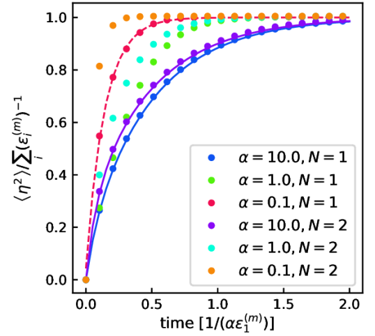
Figure 3: Time evolution of the variance of the transverse spin components in an harmonic basin when the spins have no global internal rotation symmetry ($[\mathrm{H}^{(m)},\mathrm{Q}]\neq 0$). The numerical solution is given for a different damping $\alpha$ and number of spins $N$, and for a fixed $\varepsilon_{2}^{(m)}/\varepsilon_{1}^{(m)}=6$. The solid lines indicate the analytical solutions when $\alpha\gg 1$ or $[\mathrm{H}^{(m)},\mathrm{Q}]=0$. For $N=1$ and $\alpha=0.1$, the dashed line is the analytical solution derived when $\alpha\ll 1$ in Appendix C. For $N=2$, the two additional eigenvalues are chosen to be bigger than the two first ones and $\mathrm{H}^{(m)}$ to present no global translation symmetry, giving a further speed up in the relaxation compared to $N=1$. The equilibrium time $\tau_{e}$ is at most given by $1/\alpha\varepsilon_{1}^{(m)}$.

The validation condition for the theory is

$$\Gamma\leq\tau_{e}^{-1}\;,$$ (34)

and is therefore guaranteed when

$$\Gamma\leq 2\alpha\varepsilon_{1}^{(m)}\;.$$ (35)

To understand the meaning of this result in terms of accessible damping $\alpha$, we find a higher bound for the activation rate $\Gamma$, which writes explicitly in terms of $\alpha$. By taking the dynamical mode equation for $\kappa$ (Eq. 18), and multiplying it on the left-hand side by $\hat{\bm{\zeta}}_{w_{1}}^{T}\left(\mathrm{Q}+\alpha\mathrm{I}\right)^{T}$ and noting that $(\mathrm{Q}+\alpha\mathrm{I})^{T}(\mathrm{Q}+\alpha\mathrm{I})=(1+\alpha^{2})\mathrm{I}$, we can write

$$\hat{\bm{\zeta}}_{w_{1}}^{T}\mathrm{H}^{(s)}\hat{\bm{\zeta}}_{w_{1}}=\frac{\alpha\kappa}{1+\alpha^{2}}\;.$$ (36)

As the norm of $\mathrm{H}^{(s)}$ has a lower bound given by $\varepsilon_{1}^{(s)}$, we have

$$|\kappa|\leq\frac{1+\alpha^{2}}{\alpha}|\varepsilon_{1}^{(s)}|\;,$$ (37)

which gives us the higher bound for $\Gamma$ using Eq. 27:

$$\Gamma\leq\frac{1+\alpha^{2}}{2\pi\alpha}|\varepsilon_{1}^{(s)}|\sqrt{\prod_{n=1}^{2N}\frac{\varepsilon^{(m)}_{n}}{|\varepsilon^{(s)}_{n}|}}e^{-\Delta E}\;.$$ (38)

Finally, the validation condition (Eq. 35) is satisfied for $\alpha\ll 1$ when

$$\alpha^{2}\geq\frac{1}{4\pi}\frac{|\varepsilon_{1}^{(s)}|}{\varepsilon_{1}^{(m)}}\sqrt{\prod_{n=1}^{2N}\frac{\varepsilon^{(m)}_{n}}{|\varepsilon^{(s)}_{n}|}}e^{-\Delta E}\;.$$ (39)

Consequently, the range of $\alpha$ accessible by this theory increases exponentially when the temperature decreases. Moreover, the entropic contribution coming from the square root can be of different orders of magnitude, but is of order one in the simplest case [25, 26]. In this case, when the energy barrier is, for example, one order of magnitude larger than the thermal energy scale, the theory is guaranteed to accurately predict the activation rate of systems with $\alpha$ as small as $10^{-3}$. In addition, we remind the reader that Eq. 39 is a sufficient condition obtained from a worst case, where the higher bound on $\kappa$ diverges when $\alpha\rightarrow 0$ (Eq. 37), whereas $\kappa$ is actually finite for $\alpha=0$. Therefore, one needs to validate the theory for every independent system using the more permissive condition of Eq. 35.

When the damping $\alpha$ does not satisfy the validation condition, the problem lies outside the scope of thermally activated transitions. In such a case one should consider the exact dynamical evolution with a well-defined initial condition. An approximate solution to this problem exists for a single spin [32]. It relies on computing the mean first exit time from the local minimum as an inverse activation rate. For the case of multiple spins, we can also approximate the mean first exit time from a harmonic basin even though it is not directly comparable to the inverse activation rate (see Appendix D). The result nevertheless suggests that $\Gamma$ scales as $\alpha$, and consistently vanishes with $\alpha$ when the latter goes to zero in the off-equilibrium regime not accessible by the present theory.

II.6 Activation rate for coherent transitions

The frequencies of the dynamical modes can be expressed in terms of Hessian eigenvalues for an ordered magnetic state. This means that for a coherent activation between ordered magnetic states, the computation of the prefactor to the Arrhenius law requires only knowing the Hessian spectra, as the growth rate $\kappa$ will depend directly on the Hessian spectrum at the saddle point $\{\varepsilon_{n}^{(n)}\}$. We consider here a ferromagnet whose order is maintained at the saddle point by a uniform activation and, for more complicated orders, we assume a ferromagnetic order can be obtained by a transformation into a pseudo-spin space as in Ref. [35] and demonstrated in Sec. III. For the ferromagnetic case, the lattice translational symmetry of the Hamiltonian is carried over to the Hessian $\mathrm{H}^{(s)}$, such that the spatial degrees of freedom in the dynamical equation (Eq. 17) are diagonal in Fourier space. Note that the matrix $(\mathrm{Q}+\alpha\mathrm{I})$, which also appears in the dynamical equation, is already diagonal in the spatial degrees of freedom. This will result in the dynamical mode frequencies being directly connected to pairs of Hessian eigenvalues.

We show this in the following by starting from the Fourier transform of the harmonic expansion at the saddle point which diagonalizes the spatial degrees of freedom:

$$\begin{split}\mathcal{H}^{(s)}(\bm{\zeta})&=E^{(s)}+\frac{1}{2}\sum_{\bm{q}}\bm{\zeta}_{-\bm{q}}^{T}\mathrm{H}_{\bm{q}}^{(s)}\bm{\zeta}_{\bm{q}}\\ &=E^{(s)}+\frac{1}{2}\sum_{\bm{q},\mu}\varepsilon^{(s)}_{\bm{q},\mu}(\bm{\psi}_{\bm{q},\mu}^{T}\bm{\zeta}_{\bm{q}})^{2}\;,\end{split}$$ (40)

where $\mathrm{H}_{\bm{q}}$ are $2\times 2$ matrices. The second line is obtained by projecting on the eigenvectors $\{\bm{\psi}_{\bm{q},\mu}\}$, which are labelled by the wave vector $\bm{q}$ and the orientation in the tangent plane $\mu=1,2$ (the spin degrees of freedom). Proceeding with the Fourier transform for the dynamical mode equation (Eq. 17), we find

$$\left(\mathrm{Q}+\alpha\mathrm{I}\right)_{i}\mathrm{H}_{\bm{q}}^{(s)}\bm{\zeta}_{\bm{q},w}=iw\bm{\zeta}_{\bm{q},w}\;.$$ (41)

As predicted, by solving the above eigenvalue problem, the mode frequency at $\bm{q}$ is a function of the pairs $\varepsilon^{(s)}_{\bm{q},1}$, $\varepsilon^{(s)}_{\bm{q},2}$:

$$2iw_{\bm{q},\mu}^{(s)}=\alpha\left(\varepsilon_{\bm{\bm{q}},1}^{(s)}+\varepsilon_{\bm{q},2}^{(s)}\right)\\ +(-1)^{\mu}\sqrt{\alpha^{2}\left(\varepsilon_{\bm{q},1}^{(s)}+\varepsilon_{\bm{q},2}^{(s)}\right)^{2}-4(\alpha^{2}+1)\varepsilon_{\bm{q},1}^{(s)}\varepsilon_{\bm{q},2}^{(s)}}\;.$$ (42)

When $\varepsilon_{\bm{q},1}^{(s)},\varepsilon_{\bm{q},2}^{(s)}>0$, the real parts of $iw_{\bm{q},1}^{(s)}$ and $iw_{\bm{q},2}^{(s)}$ are positive, and the associated dynamical modes are stable, forming decaying spin waves. The same result can be obtained at the minimum. We note now that in the ferromagnetic case the dynamical instability arises at the saddle point from the subspace at $\bm{q}=\bm{0}$ ($\varepsilon_{\bm{0},1}^{(s)}<0$ and $\varepsilon_{\bm{0},2}^{(s)}>0$), such that the prefactor (Eq. 28) is an explicit function of Hessian eigenvalues:

$$\nu_{coh}=\frac{|iw_{\bm{0},1}^{(s)}|}{2\pi}\sqrt{\prod_{\bm{q}}\frac{\varepsilon_{\bm{q},1}^{(m)}\varepsilon_{\bm{q},2}^{(m)}}{|\varepsilon_{\bm{q},1}^{(s)}|\varepsilon_{\bm{q},2}^{(s)}}}\;.$$ (43)

When the damping $\alpha\ll 1$, we note from Eq. 42 that

$$|w_{\bm{q},1}^{(s)}w_{\bm{q},2}^{(s)}|=|\varepsilon_{\bm{q},1}^{(s)}|\varepsilon_{\bm{q},2}^{(s)}\;,$$ (44)

allowing us to express the prefactor only in terms of the dynamical modes:

$$\nu_{coh}=\frac{|iw_{\bm{0},1}^{(s)}|}{2\pi}\sqrt{\prod_{\bm{q}}\frac{|w_{\bm{q},1}^{(m)}w_{\bm{q},2}^{(m)}|}{|w_{\bm{q},1}^{(s)}w_{\bm{q},2}^{(s)}|}}\;.$$ (45)

Furthermore, we observe that the entropic contribution given by the square root is only made of spin wave frequencies. In addition, when the damping is such that $\alpha\ll\sqrt{4|\varepsilon_{\bm{0},1}^{(s)}|/\varepsilon_{\bm{0},2}^{(s)}}$, we have $|iw_{\bm{0},1}^{(s)}|=\sqrt{|\varepsilon_{\bm{q},1}^{(s)}|\varepsilon_{\bm{q},2}^{(s)}}$. This corresponds to the underdamped regime, as the prefactor becomes independent of $\alpha$.

III Coherent activation of antiferromagnetic chains

In this section, we exemplify the theory and derive a simple analytical expression for the prefactor $\nu$ of the activation rate to directly evaluate its dependence on the Hamiltonian parameters, the damping and the system size. We consider the following Hamiltonian:

$$\mathcal{H}=\frac{J}{2}\sum_{<i,j>}\bm{s}_{i}\bm{s}_{j}-K\sum_{i}(s_{i}^{y})^{2}+D\sum_{i}(s_{i}^{z})^{2}\;,$$ (46)

with $J>0$ a nearest neighbor antiferromagnetic exchange, $K>0$ an easy-axis anisotropy and $D>0$ an easy-plane anisotropy. In addition, we consider the exchange dominated regime where $\sqrt{J/K}$, $\sqrt{J/D}\geq N$. In this regime, the lowest energy transition between the two model antiferromagnetic ordered ground states along $y$ corresponds to a coherent transition, as illustrated in Fig. 4.

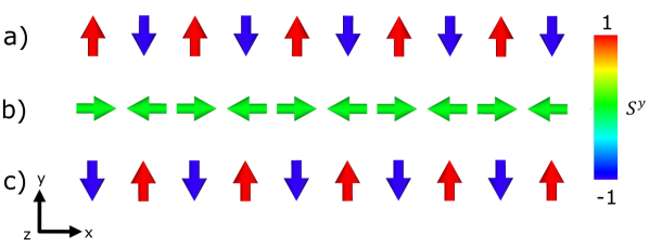
Figure 4: a) Ground state (global minimum of the energy) of the Hamiltonian in Eq. 46. b) Lowest energy activated state (saddle point) between the time reversal symmetric ground states in the exchange dominated regime ($\sqrt{J/K}$, $\sqrt{J/D}\geq N$) c) Time reversal ground state corresponding to the final state of the transition (second global minimum).

To make use of the results obtained for the ferromagnetic order in section II.6, we first rewrite $\mathcal{H}$ in a pseudo spin space, where the order is effectively ferromagnetic [35]. The pseudo spin variables are obtained as $\bm{\sigma}_{i}=R_{z}(Qr_{i})\bm{s}_{i}$ where $R_{z}(\theta)$ is a rotation matrix about the $z$-axis of $\theta$, $Q=\pi/a$ is the antiferromagnetic propagation vector and $a$ the lattice parameter, such that $\mathcal{H}$ becomes:

$$\mathcal{H}=\frac{J}{2}\sum_{<i,j>}\left(-\sigma_{i}^{x}\sigma_{j}^{x}-\sigma_{i}^{y}\sigma_{j}^{y}+\sigma_{i}^{z}\sigma_{j}^{z}\right)\\ -K\sum_{i}(\sigma_{i}^{y})^{2}+D\sum_{i}(\sigma_{i}^{z})^{2}\;.$$ (47)

The harmonic expansion (Eq. 8) can then be evaluated (Eq. 6), Fourier transformed (Eq. 40) and diagonalizeed in the tangent plane. At the saddle point, this gives the spectrum of the Hessian $\mathrm{H}^{(s)}$:

$$\varepsilon^{(s)}_{q,\mu}=\varepsilon_{q,\mu}+\Delta\varepsilon_{\mu}^{(s)}\;,$$ (48)

with the dispersive exchange contribution:

$$\varepsilon_{q,\mu}=2J\left[1+(-1)^{\mu}\cos(qa)\right]\;,$$ (49)

and the constant anisotropy contribution:

$$\Delta\varepsilon_{\mu}^{(s)}=2(-\delta_{\mu 1}K+\delta_{\mu 2}D)\;.$$ (50)

The exchange contribution in Eq. 49 is plotted in Fig. 5a. The underdamped dynamic dispersion relation obtained by inserting $\varepsilon_{q,\mu}$ into the conservative part ($\alpha=0$) of Eq. 42, i.e.

$$w_{q,\mu}=(-1)^{\mu}2J\sqrt{1-\cos^{2}(qa)}\;,$$ (51)

is the familiar antiferromagnetic spin wave dispersion (Fig. 5b).

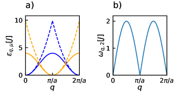
Figure 5: a) Two branches corresponding to the exchange contribution to the spectrum of the Hessian at the minimum and at the saddle point (solid lines) and the two approximated branches used in Eq. 56 (dashed lines) b). One branch of the corresponding dynamic dispersion relation (the other is mirrored with respect to the $q$-axis).

To obtain the Hessian spectrum at the minimum we can repeat the procedure:

$$\varepsilon^{(m)}_{q,\mu}=\varepsilon_{q,\mu}+\Delta\varepsilon_{\mu}^{(m)}\;,$$ (52)

with the same exchange contribution as in Eq. 49 and a different anisotropy contribution:

$$\Delta\varepsilon_{\mu}^{(m)}=2(K+\delta_{\mu 2}D)\;.$$ (53)

We now develop the prefactor $\nu$ (Eq. 43) knowing the Hessian sprectrum at the saddle point (Eq. 48) and at the minimum (Eq. 52). In particular, we want to evaluate the following product:

$$\prod_{q,\mu}\frac{\varepsilon_{\bm{q},\mu}^{(m)}}{|\varepsilon_{\bm{q},\mu}^{(s)}|}=\prod_{q,\mu}\left(\frac{\varepsilon_{q,\mu}+\Delta\varepsilon_{\mu}^{(m)}}{|\varepsilon_{q,\mu}+\Delta\varepsilon_{\mu}^{(s)}|}\right)\;.$$ (54)

For a given direction $\mu$, we treat separately the factors where $\varepsilon_{q,\mu}$ vanishes and assume that for the other wavevectors we can expand to leading order in $\Delta\varepsilon_{\mu}^{(m)}/\varepsilon_{q,\mu}^{0}$ and $\Delta\varepsilon_{\mu}^{(s)}/\varepsilon_{q,\mu}^{0}$ as suggested by the exchange dominated regime $J/K$, $J/D\geq N^{2}$. This gives

$$\prod_{\varepsilon_{q,\mu}\neq 0}\left(\frac{\varepsilon_{q,\mu}+\Delta\varepsilon_{\mu}^{(m)}}{\varepsilon_{q,\mu}+\Delta\varepsilon_{\mu}^{(s)}}\right)\\ \approx\exp\left[\left(\Delta\varepsilon_{\mu}^{(m)}-\Delta\varepsilon_{\mu}^{(s)}\right)\sum_{\varepsilon_{q,\mu}\neq 0}\frac{1}{\varepsilon_{q,\mu}}\right]\;.$$ (55)

The sum in the exponent is independent of $\mu$ and can be approximated by expanding to quadratic order about the minimum (see Fig. 5a):

$$\begin{split}\sum_{\varepsilon_{q,\mu}>0}^{2\pi/a}\frac{1}{\varepsilon_{q,\mu}}&\approx\frac{2}{Ja^{2}}\sum_{q>0}^{\pi/a}\frac{1}{q^{2}}\\ &=\frac{2N^{2}}{J(2\pi)^{2}}\sum_{n=1}^{N}\frac{1}{n^{2}}\\ &\approx\frac{N^{2}}{12J}\;,\end{split}$$ (56)

with the last approximation obtained by considering that the system size $N$ is large and taking the result for the infinite sum. Finally, we insert this result into the product (Eq. 55), and obtain the following prefactor contribution by factoring out the terms where $\varepsilon_{q,1}$ and $\varepsilon_{q,2}$ vanish:

$$\prod_{q,\mu}\frac{\varepsilon_{q,\mu}^{(m)}}{|\varepsilon_{\bm{q},\mu}^{(s)}|}\approx\prod_{\mu}\frac{\Delta\varepsilon_{\mu}^{(m)}}{|\Delta\varepsilon_{\mu}^{(s)}|}\exp\left[\left(\Delta\varepsilon_{\mu}^{(m)}-\Delta\varepsilon_{\mu}^{(s)}\right)\frac{N^{2}}{12J}\right]\;.$$ (57)

Using this result allows to write explicitly the prefactor:

$$\nu_{AF}=\frac{|\kappa|}{\pi}\sqrt{\frac{(K+D)}{D}}\exp\left(\frac{N^{2}K}{4J}\right)$$ (58)

with the absolute growth rate $|\kappa|$ at leading order in $K/J$ and $D/J$:

$$|\kappa|\approx 2\alpha J\left(\sqrt{1+\frac{2K(1+\alpha^{2})}{J\alpha^{2}}}-1\right)\;.$$ (59)

The prefactor $\nu_{AF}$ is multiplied by $2$ compared to $\nu$ in Eq. 43 to account for the two equivalent transitions. To conclude, we consider additionally the Arrhenius exponential where $\Delta E=NK$ and write $\Gamma$ as

$$\Gamma_{AF}=\nu_{AF}e^{-NK}\;.$$ (60)

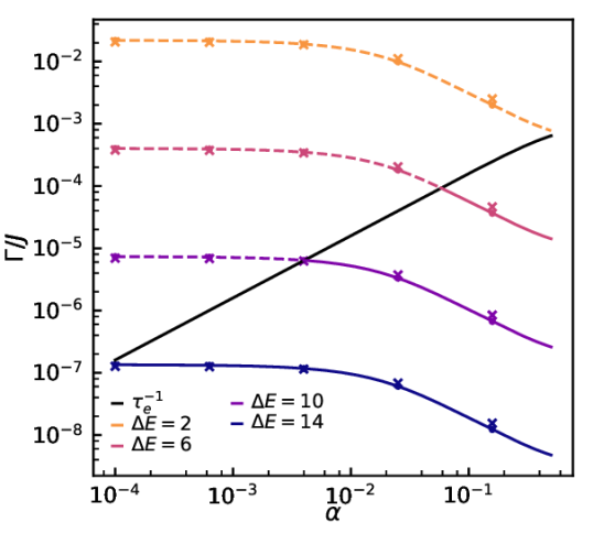
Figure 6: For $\sqrt{J/D}=2\sqrt{J/K}=100$ and $N/\sqrt{J/K}=1$, approximated activation rate $\Gamma_{AF}$ as a function of $\alpha$. For comparison, we show the numerical results computed according to Eq. 28 for a chain with open boundary conditions by crosses and periodic boundary conditions by dots. The black line denotes the inverse of the critical equilibrium time $\tau_{e}^{-1}$ above which the theory breaks down.

In Fig. 6, we plot $\Gamma_{AF}/J$ as a function of $\alpha$ for a system defined by $\sqrt{J/D}=2\sqrt{J/K}=100$ and $N/\sqrt{J/K}=1$. By also plotting the numerical results computed with the general expression for $\Gamma$ (Eq. 27), we observe that $\Gamma_{AF}$ is a good prediction. In particular, despite the expansion of the product in $\Delta\varepsilon_{\mu}/\varepsilon_{q,\mu}^{0}$ (Eq. 55) and the expansion of the spectra $\varepsilon_{q,\mu}$ about the minima (Eq. 56), the prediction is perfectly accurate for a chain with periodic boundary conditions. Besides, the error in predicting a chain with open boundary conditions is far smaller than the variation induced by relevant parameter changes.

Concerning the dependence in $\alpha$, we can first observe the underdamped regime for $\alpha\ll\sqrt{4|\varepsilon_{\bm{0},1}^{(s)}|/\varepsilon_{\bm{0},2}^{(s)}}\approx\sqrt{2K/J}$ as previously defined, i.e. where $\Gamma$ is constant and in particular $|\kappa|=|iw_{\bm{0},1}|=\sqrt{|\varepsilon_{\bm{0},1}^{(s)}|\varepsilon_{\bm{0},2}^{(s)}}\approx\sqrt{8KJ}$. In contrast, when $\alpha\gg\sqrt{2K/J}$, we see a regime where $\Gamma\propto\alpha^{-1}$. Therefore, $\Gamma$ is sensitive to $\alpha$ and an error in the experimental evaluation of $\alpha$ can affect $\Gamma$ as much. Note that this regime is not relevant for ferromagnetic systems with an almost-axially symmetric anisotropy. Indeed, it appears here for $\alpha\ll 1$ because the antiferromagnetic order splits the Hessian spectra in two distant branches (Fig. 5a) shifting the onset of the underdamped regime well below $\alpha=1$.

In order to validate the results, we look at the validation condition found in Sec. II.5 and plot with a solid black line in Fig. 6 the inverse of the time to reach equilibrium at the minimum, i.e. $\tau_{e}^{-1}=2\alpha\varepsilon_{\bm{0},1}^{(m)}=4\alpha K$. This sets the upper bound on the activation rates that can be predicted with this theory. As demonstrated in Sec. II.5, despite the possible entropic effect from the ratio of eigenvalues, the lowest accessible $\alpha$ decreases exponentially with $\Delta E$, covering $\alpha$ down to $10^{-4}$ when $\Delta E=14$.

Finally, the length of the chain $N$ modifies $\Gamma$, by affecting both the Arrhenius exponential $e^{-\Delta E}$ and $\nu$ exponentially through the entropic contribution. Nonetheless, for the regime considered here ($N\leq\sqrt{J/K}$), the change in $\nu_{AF}$ with $N$ does not exceed a factor of $e^{0.25}\approx 1.3$ when $N^{2}=\sqrt{J/K}$ (Eq. 58). In addition, despite the opposite trend of $\nu_{AF}$ and $e^{-\Delta E}$ with $N$, a regime where $\Gamma$ increases with $N$, paradoxical from the perspective of the Arrhenius exponential only, cannot be predicted. Indeed, $\Gamma^{\prime}(N)>0$ requires $NK>2JK$ and we already assume $NK\leq\sqrt{JK}$ from the exchange dominated regime. Combining these two inequalities implies that $NK=\Delta E<1$ and the validation condition becomes approximately $|\kappa|\lesssim\alpha K$. The latter is satisfied only in the experimentally irrelevant overdamped regime of $\alpha\gtrsim 1$. In conclusion, in the present investigation, $\Gamma$ always decreases exponentially with the system size.

IV Discussion and concluding remarks

We have demonstrated that using the tangent spaces of the spin configuration allows us to develop a harmonic theory straightforwardly to find the activation rate for thermally activated transitions in spin systems. In the spirit of the work of Langer [18], we have assumed equilibrium in the initial minimum. Considering the complete spin dynamics with the thermal fluctuations and the dissipation essential for the system to approach an activated state (a saddle point) and reach equilibrium, the activation rate was evaluated as the integral of the probability density flux at the saddle point. The calculation relies on using the appropriate boundary conditions, consistent with equilibrium in the initial minimum, and imposing the probability density flux parallel to the only unstable dynamical mode. The latter originates from the average dynamics, i.e. the deterministic part of the stochastic Landau-Lifschitz (LL) dynamics.

The resulting Arrhenius law describing the activation rate is the same as in Ref. [18]. The prefactor of the Arrhenius law depends on the growth rate of the unstable dynamical mode, which can now be understood from the constraint on the probability density flux. This implies that the prefactor depends on the Gilbert damping parameter $\alpha$ through this growth rate. Such a dependence in $\alpha$ is absent in the spin activation rate theory of Ref. [23], as the thermal fluctuations in the dynamics are neglected. Moreover, the prefactor contains an entropic contribution from the product of eigenvalues at the minimum and at the saddle point, allowing for a non-trivial dependence of the prefactor on system size. Finally, the prefactor is independent of the temperature in the absence of zero-modes. However, in agreement with the original work of Brown for a single spin with a uniaxial anisotropy [15], a factor containing the inverse square root of the temperature will emerge when the axial zero-mode at the saddle point is taken into account.

To validate the theory, we computed the time to reach equilibrium in a minimum basin and compared it with the inverse activation rate. We found it proportional to $\alpha$ and therefore vanishing when $\alpha\rightarrow 0$. In contrast, the LL dynamics is well-defined when $\alpha\rightarrow 0$ such that the aforementioned growth rate and the activation rate reach a finite non-zero value. This implies that the theory necessarily breaks down below some $\alpha$. Nevertheless, by looking at the scale of the activation rate, we found that the theory can cover a large range of experimental values of $\alpha\ll 1$ when the energy barrier is larger than the thermal energy, in contrast to what is predicted in Ref. [16]. Predicting the activation rate when the energy barrier is too small and equilibrium in the initial minimum seems à priori out of the scope of the considered thermally activated transitions, as it should involve exact trajectories in phase space. An approximate solution to this problem exists for a single spin in Ref. [32], but was not found to be transferable to systems with multiple spins.

When the activation is coherent, i.e. maintains an order through the transition, we have developed the exact dependence of the growth rate to the damping $\alpha$. We found that for $\alpha\ll 1$, the prefactor writes directly in terms of spin wave frequencies. In this regime, the entropic contribution to the prefactor indicates for instance that softer spin wave excitations in the convex region at the saddle point compared to the ones at the minimum increase the prefactor and therefore the activation rate. We have further seen that the onset of the underdamped regime, where the activation rate is independent of $\alpha$, depends on the ratio of eigenvalues along the two transverse spin components at the saddle point. In particular, the onset can be shifted down from $\alpha\approx 1$ in the presence of a non-axially symmetric anisotropy in the Hamiltonian or when the transition is between non-ferromagnetic order, as observed with the antiferromagnetic chain in Sec. III.

The antiferromagnetic spin chain in Sec. III has exemplified these results and showcased an explicit calculation of the prefactor regarding of system size and parameters. In particular, it was found that, due to the entropic contribution, the prefactor increases exponentially with the easy-axis anisotropy, which sets the energy barrier $\Delta E$. Following Ref. [26], this dependence would suggest that the prefactor satisfies the Meyer-Neldel compensation rule: $\ln(\nu)=\ln(\nu_{0})+\Delta E/E_{0}+cst$ [36, 37]. However, the prefactor was also found to depend exponentially on the square of the system size while the energy barrier was proportional to the system size, invalidating the Meyer-Neldel rule and the existence of a simple relationship between the prefactor and the energy barrier. In addition, knowledge of the exact analytical dependence of the prefactor on the system size is itself an important result, since only few studies in the literature have addressed this problem numerically, showing various results according to the systems and regimes investigated [21, 22, 24].

This paper presents a robust and controlled framework to investigate the activation rate for local or extensive thermally activated transitions in order or disordered spin systems. In particular, the present authors have developed this approach to predict the reversal time of a magnetic Co nanoparticle including defects, going therefore beyond Brown’s seminal work and solving a long-lasting paradox in the search for magnetic stability at the nanoscale [38].

Appendix A Existence and unicity of a real unstable dynamical mode

Existence. The existence of a real negative dynamical mode is guaranteed by looking individually at the determinant of $\mathrm{H}^{(s)}$ and $(\mathrm{Q}+\alpha\mathrm{I})$. Indeed, we have:

$$\det\left[(\mathrm{Q}+\alpha\mathrm{I})\mathrm{H}^{(s)}\right]=\det\left(\mathrm{Q}+\alpha\mathrm{I}\right)\det\left(\mathrm{H}^{(s)}\right)<0\;,$$ (61)

since $\det\left(\mathrm{H}^{(s)}\right)<0$ due to the presence of a unique negative eigenvalue (Eq. 15) and $\det\left(\mathrm{Q}+\alpha\mathrm{I}\right)=(1+\alpha^{2})^{N}>0$ (Eq. 10). But as $(\mathrm{Q}+\alpha\mathrm{I})\mathrm{H}^{(s)}$ is real, its complex modes come by conjugate pairs making a positive contribution to the determinant and only an odd number (non-zero) of real negative modes is compatible with Eq. 61.

Unicity. We prove unicity by contradiction and start by assuming the existence of multiple real unstable dynamical modes. We consider in particular two distinct: $\kappa_{1}=iw_{1}<0$ and $\kappa_{2}=iw_{2}<0$ such that

$$\begin{split}(\mathrm{Q}+\alpha\mathrm{I})\mathrm{H}^{(s)}\hat{\bm{\zeta}}_{w_{1}}=\kappa_{1}\hat{\bm{\zeta}}_{w_{1}}\;,\\ (\mathrm{Q}+\alpha\mathrm{I})\mathrm{H}^{(s)}\hat{\bm{\zeta}}_{w_{2}}=\kappa_{2}\hat{\bm{\zeta}}_{w_{2}}\;.\end{split}$$ (62)

$\hat{\bm{\zeta}}_{w_{1}}$ and $\hat{\bm{\zeta}}_{w_{2}}$ are the normalized modes which are not necessarily perpendicular since $(\mathrm{Q}+\alpha\mathrm{I})\mathrm{H}^{(s)}$ is not symmetric (see Fig. 7). On the one hand, multiplying the first (resp. second) equation to the left by $\hat{\bm{\zeta}}_{w_{1}}^{T}(\mathrm{Q}+\alpha\mathrm{I})^{T}$ [resp. $\hat{\bm{\zeta}}_{w_{2}}^{T}(\mathrm{Q}+\alpha\mathrm{I})^{T}$] and noting that $(\mathrm{Q}+\alpha\mathrm{I})^{T}(\mathrm{Q}+\alpha\mathrm{I})=(1+\alpha^{2})\mathrm{I}$ gives

$$\begin{split}\hat{\bm{\zeta}}_{w_{1}}^{T}\mathrm{H}^{(s)}\hat{\bm{\zeta}}_{w_{1}}=\frac{\alpha\kappa_{1}}{1+\alpha^{2}}\;,\\ \hat{\bm{\zeta}}_{w_{2}}^{T}\mathrm{H}^{(s)}\hat{\bm{\zeta}}_{w_{2}}=\frac{\alpha\kappa_{2}}{1+\alpha^{2}}\;.\end{split}$$ (63)

On the other hand, multiplying the first (resp. second) equation in 62 by $\hat{\bm{\zeta}}_{w_{2}}^{T}(\mathrm{Q}+\alpha\mathrm{I})^{T}$ [resp. $\hat{\bm{\zeta}}_{w_{1}}^{T}(\mathrm{Q}+\alpha\mathrm{I})^{T}$] yields

$$\begin{split}\hat{\bm{\zeta}}_{w_{2}}^{T}\mathrm{H}^{(s)}\hat{\bm{\zeta}}_{w_{1}}=\frac{\kappa_{1}}{1+\alpha^{2}}\hat{\bm{\zeta}}_{w_{2}}^{T}(\mathrm{Q}^{T}+\alpha\mathrm{I})\hat{\bm{\zeta}}_{w_{1}}\;,\\ \hat{\bm{\zeta}}_{w_{1}}^{T}\mathrm{H}^{(s)}\hat{\bm{\zeta}}_{w_{2}}=\frac{\kappa_{2}}{1+\alpha^{2}}\hat{\bm{\zeta}}_{w_{1}}^{T}(\mathrm{Q}^{T}+\alpha\mathrm{I})\hat{\bm{\zeta}}_{w_{2}}\;.\end{split}$$ (64)

Due to the symmetry of $\mathrm{H}^{(s)}$, these two equations are equal and in particular by equalizing the two right-hand side, we obtain

$$\hat{\bm{\zeta}}_{w_{1}}^{T}\mathrm{Q}^{T}\hat{\bm{\zeta}}_{w_{2}}=\alpha\frac{\kappa_{1}-\kappa_{2}}{\kappa_{1}+\kappa_{2}}\hat{\bm{\zeta}}_{w_{1}}^{T}\hat{\bm{\zeta}}_{w_{2}},$$ (65)

which implies

$$\hat{\bm{\zeta}}_{w_{1}}^{T}\mathrm{H}^{(s)}\hat{\bm{\zeta}}_{w_{2}}=\frac{2\alpha\kappa_{1}\kappa_{2}}{(1+\alpha^{2})(\kappa_{1}+\kappa_{2})}\hat{\bm{\zeta}}_{w_{1}}^{T}\hat{\bm{\zeta}}_{w_{2}}\;.$$ (66)

Finally, with Eq. 63 and 66, we can evaluate the norm with respect to $\mathrm{H}^{(s)}$ of a non-zero vector $\bm{\zeta}\in span(\hat{\bm{\zeta}}_{w_{1}},\hat{\bm{\zeta}}_{w_{2}})$. In particular, we write $\bm{\zeta}=x\hat{\bm{\zeta}}_{w_{1}}+y\hat{\bm{\zeta}}_{w_{2}}$ with $(x,y)^{T}\in\mathbb{R}^{2}$\$\{\bm{0}\}$, such that

$$\begin{split}\bm{\zeta}^{T}\mathrm{H}^{(s)}\bm{\zeta}&=x^{2}\hat{\bm{\zeta}}_{w_{1}}^{T}\mathrm{H}^{(s)}\hat{\bm{\zeta}}_{w_{1}}+y^{2}\hat{\bm{\zeta}}_{w_{2}}^{T}\mathrm{H}^{(s)}\hat{\bm{\zeta}}_{w_{2}}+2xy\hat{\bm{\zeta}}_{w_{1}}^{T}\mathrm{H}^{(s)}\hat{\bm{\zeta}}_{w_{2}}\\ &=\frac{\alpha}{1+\alpha^{2}}\left(x^{2}\kappa_{1}+y^{2}\kappa_{2}+4xy\hat{\bm{\zeta}}_{w_{1}}^{T}\hat{\bm{\zeta}}_{w_{2}}\frac{\kappa_{1}\kappa_{2}}{\kappa_{1}+\kappa_{2}}\right)\\ &=\frac{\alpha}{1+\alpha^{2}}\left[\frac{(x\kappa_{1}\hat{\bm{\zeta}}_{w_{1}}+y\kappa_{2}\hat{\bm{\zeta}}_{w_{2}})^{2}+(x\hat{\bm{\zeta}}_{w_{1}}+y\hat{\bm{\zeta}}_{w_{2}})^{2}\kappa_{1}\kappa_{2}}{\kappa_{1}+\kappa_{2}}\right]\;.\end{split}$$ (67)

The last equation is written to highlight the sign of the norm which is always negative due to the denominator. In other words, we find that $\mathrm{H}^{(s)}$ is at least negative definite in a two-dimensional subspace. However, this is a contradiction with the fact that $\mathrm{H}^{(s)}$ has a unique negative eigenvalue, as depicted in Fig. 7. We conclude that there cannot be multiple real unstable dynamical modes.

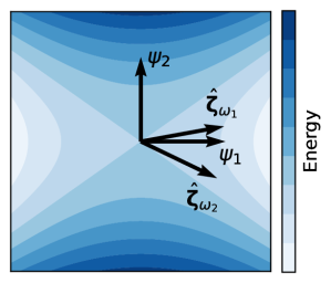
Figure 7: If we assume $\hat{\bm{\zeta}}_{w_{1}}$ and $\hat{\bm{\zeta}}_{w_{2}}$ to be two negative real dynamical modes (not necessarily pependicular since $(\mathrm{Q}+\alpha\mathrm{I})\mathrm{H}^{(s)}$ is not symmetric), then $\mathrm{H}^{(s)}$ must be negative definite on the two-dimensional subspace defined by $span(\hat{\bm{\zeta}}_{w_{1}},\hat{\bm{\zeta}}_{w_{2}})$ (Eq. 67). However, as illustrated by $\mathcal{H}^{(s)}$ on $span(\hat{\bm{\zeta}}_{w_{1}},\hat{\bm{\zeta}}_{w_{2}})$, $\mathrm{H}^{(s)}$ is defined with only a one-dimensional subspace of negative curvature along $\bm{\psi}_{1}$.

Appendix B Computing the activation rate from the probability flux

The activation rate (Eq. 26) can be written explicitly as,

$$\Gamma=\sqrt{\frac{(1+\alpha^{2})|\kappa|}{2\pi\alpha}}|\bm{\psi}_{1}^{T}\hat{\bm{\zeta}}_{w_{1}}|\\ \times\frac{e^{-E^{(s)}}}{Z^{(m)}}\int_{\bm{\psi}_{1}^{T}\bm{\zeta}=0}\exp\left[-\frac{1}{2}\bm{\zeta}^{T}\mathrm{Q}\bm{\zeta}\right]d\bm{\zeta}\;,$$ (68)

with the symmetric matrix $\mathrm{Q}$ that can be expanded in the basis of the Hessian $\mathrm{H}^{(s)}$, $\{\bm{\psi}_{n}\}$:

$$\mathrm{Q}_{ln}=\delta_{ln}\varepsilon_{n}^{(s)}+\frac{(1+\alpha^{2})}{\alpha|\kappa|}\varepsilon_{l}^{(s)}\varepsilon_{n}^{(s)}({\bm{\psi}}_{l}^{T}\hat{\bm{\zeta}}_{w_{1}})({\bm{\psi}}_{n}^{T}\hat{\bm{\zeta}}_{w_{1}})\;.$$ (69)

This form is obtained by writing $u^{2}$ in Eq. 25 with the definition of Eq. 21, transforming with Eq. 18 and expanding. The integral in Eq. 68 is evaluated on the subspace $\bm{\psi}_{1}^{T}\bm{\zeta}=0$, corresponding to the indices $l,n\geq 2$. On this subspace, the eigenvalues $\varepsilon_{n}^{(s)}$ are positive and, as in Ref. [18], we can symmetrize the last expression:

$$\mathrm{Q}_{ln}=\sqrt{\varepsilon_{l}^{(s)}}\mathrm{S}_{ln}\sqrt{\varepsilon_{n}^{(s)}}\;.$$ (70)

with the symmetric matrix

$$\mathrm{S}_{ln}=\delta_{ln}+\frac{(1+\alpha^{2})}{\alpha|\kappa|}\sqrt{\varepsilon_{l}^{(s)}\varepsilon_{n}^{(s)}}(\bm{\psi}_{l}^{T}\hat{\bm{\zeta}}_{w_{1}})(\bm{\psi}_{n}^{T}\hat{\bm{\zeta}}_{w_{1}})\;.$$ (71)

Therefore the integral in Eq. 68 can be evaluated as $\sqrt{(2\pi)^{2N-1}/p\prod_{n\geq 2}\varepsilon_{n}^{(s)}}$ where $p$ is the product of the eigenvalues of $\mathrm{S}$ on the subspace where $l,n\geq 2$. To find $p$, we note on the one hand that $v_{n}=\sqrt{\varepsilon_{n}^{(s)}}(\bm{\psi}_{n}^{T}\hat{\bm{\zeta}}_{w_{1}})$ is an eigendirection of $\mathrm{S}$:

$$\sum_{n\geq 2}\mathrm{S}_{ln}v_{n}=\left(1+\frac{1+\alpha^{2}}{\alpha|\kappa|}\sum_{n\geq 2}\varepsilon_{n}^{(s)}(\bm{\psi}_{n}^{T}\hat{\bm{\zeta}}_{w_{1}})^{2}\right)v_{l}\;,$$ (72)

and that all the other eigendirections are perpendicular and hence have an eigenvalue of 1. On the other hand, we have:

$$\begin{split}\sum_{n\geq 1}\varepsilon_{n}^{(s)}(\bm{\psi}_{n}^{T}\hat{\bm{\zeta}}_{w_{1}})^{2}&=\hat{\bm{\zeta}}_{w_{1}}^{T}\mathrm{H}\hat{\bm{\zeta}}_{w_{1}}\\ &=\kappa\hat{\bm{\zeta}}_{w_{1}}^{T}(\mathrm{Q}+\alpha\mathrm{I})^{-1}\hat{\bm{\zeta}}_{w_{1}}\\ &=\frac{\alpha\kappa}{1+\alpha^{2}}\;,\end{split}$$ (73)

with the second line obtained via Eq. 18, and the third via $(1+\alpha^{2})(\mathrm{Q}+\alpha\mathrm{I})^{-1}=(\mathrm{Q}+\alpha\mathrm{I})$ and the antisymmetry of $\mathrm{Q}$. Therefore, by inserting this result into the only non-unitary eigenvalue in Eq. 72 which corresponds to $p$, we get

$$p=\frac{1+\alpha^{2}}{\alpha|\kappa|}|\varepsilon_{1}^{(s)}|(\bm{\psi}_{1}^{T}\hat{\bm{\zeta}}_{w_{1}})^{2}$$ (74)

We can finally obtain the integral in Eq. 68 as,

$$\int_{\bm{\psi}_{1}^{T}\bm{\zeta}=0}\exp\left[-\frac{1}{2}\bm{\zeta}^{T}\mathrm{Q}\bm{\zeta}\right]d\bm{\zeta}\\ =\frac{1}{|\bm{\psi}_{1}^{T}\hat{\bm{\zeta}}_{w_{1}}|}\sqrt{\frac{\alpha|\kappa|}{2\pi(1+\alpha^{2})}\prod_{n\geq 1}\frac{2\pi}{|\varepsilon_{n}^{(s)}|}}\;.$$ (75)

Using the above result and Eq. 14, the activation rate in Eq. 68 can be written as a closed-form expression in Eq. 27.

Appendix C Spin relaxation in a harmonic basin

We wish to determine the time evolution of the variance of the transverse components of a spin in an harmonic basin when $[\mathrm{H}^{(m)},\mathrm{Q}]\neq 0$. Eq. 32 can be rewritten by expanding the exponentials in the integrand in series and convoluting them using the Cauchy product rule, giving

$$\left<\bm{\eta}^{2}\right>=2\alpha\int_{u=0}^{t}\sum_{k=0}^{\infty}\sum_{l=0}^{k}\frac{(u-t)^{k}}{l!(k-l)!}\sum_{n=1}^{2}\bm{\phi}_{n}^{T}\left(\alpha\mathrm{H}^{(m)}-\mathrm{H}^{(m)}\mathrm{Q}\right)^{l}\left(\alpha\mathrm{H}^{(m)}+\mathrm{Q}\mathrm{H}^{(m)}\right)^{k-l}\bm{\phi}_{n}du\;.$$ (76)

We solve this problem in the relevant small damping regime $\alpha\ll 1$ by keeping terms up to first order in $\alpha$. The development is trivial but tedious and involves considering, independently, the zero order case and the first order case when an $\alpha$ comes out from the first and the second pair of parentheses. Also one needs to keep in mind that for the two-dimensional transverse space of the single spin system we have,

$$\bm{\phi}_{n}^{T}\mathrm{Q}^{k}\bm{\phi}_{n}=\left(\frac{1+(-1)^{k}}{2}\right)(-1)^{k/2}\;.$$ (77)

After some algebra, we can obtain by dropping the index of the minimum for the eigenvalues of $\mathrm{H}^{(m)}$:

$$\left<\bm{\eta}^{2}(t)\right>\approx 2\alpha\int_{u=0}^{t}du\left[\frac{(\varepsilon_{1}+\varepsilon_{2})^{2}}{2\varepsilon_{1}\varepsilon_{2}}-\frac{(\varepsilon_{2}-\varepsilon_{1})^{2}}{2\varepsilon_{1}\varepsilon_{2}}\cos(2\sqrt{\varepsilon_{1}\varepsilon_{2}}(u-t))\right]\left[1+\alpha(\varepsilon_{1}+\varepsilon_{2})(u-t)\right]\;.$$ (78)

We retrieve an exponential from this expansion using $1+\alpha(\varepsilon_{1}+\varepsilon_{2})(u-t)\approx\exp[\alpha(\varepsilon_{1}+\varepsilon_{2})(u-t)]$ such that the integral converges at large time. We can find the equilibrium time by looking at the solution to leading order in $\alpha$, giving

$$\left<\bm{\eta}^{2}(t)\right>\approx\frac{\varepsilon_{1}+\varepsilon_{2}}{\varepsilon_{1}\varepsilon_{2}}\left[1-e^{-\alpha(\varepsilon_{1}+\varepsilon_{2})t}\right]\\ -\frac{\alpha(\varepsilon_{2}-\varepsilon_{1})^{2}}{2(\varepsilon_{1}\varepsilon_{2})^{3/2}}\sin(2\sqrt{\varepsilon_{1}\varepsilon_{2}}t)e^{-\alpha(\varepsilon_{1}+\varepsilon_{2})t}\;.$$ (79)

The solution is composed of a monotounously converging term that matches the solution of the problem when $[\mathrm{H}^{(m)},\mathrm{Q}]=0$ and $\varepsilon_{1}=\varepsilon_{2}$ (Eq. 33) and a second damped oscillating term, which exists only when $[\mathrm{H}^{(m)},\mathrm{Q}]\neq 0$. Both terms have the same relaxation time, such that the equilibrium time (the longest relaxation time) is given by $\tau_{e}=1/\alpha(\varepsilon_{1}+\varepsilon_{2})$.

Appendix D Mean first exit time

When the damping $\alpha$ is too small to satisfy the validation condition (Eq. 35), the system cannot be considered in equilibrium before crossing the saddle point. Alternatively however, we know that when the longest precessional time $\sim 1/\varepsilon_{1}^{(m)}$ is shorter than the shortest relaxation time, defined by $1/2\alpha\varepsilon_{2N}^{(m)}$ according to Eq. 33, the system evolves with quasi-deterministic precessions. This occurs in the local minimum when $\alpha\ll\varepsilon_{1}^{(m)}/\varepsilon_{2N}^{(m)}$. For a system with a single spin, this quasi-deterministic evolution implies essentially that once the system reaches the energy barrier it will visit the saddle point. With this convenient feature the activation rate can be approximated using the concept of mean first exit time [32]. Unfortunately, the system is not guaranteed to visit the saddle point when the energy barrier is reached in more dimensions, as the precession may occur in a different space than the one of the saddle point.

Nevertheless, we define and approximate here the mean first exit time solely based on the harmonic expansion at the minimum and find the important scaling which suggests that $\Gamma\propto\alpha$ in this regime.

We consider the first exit time $\tau_{1}(\bm{\eta})$ has the time to reach the iso-energy manifold of the saddle point starting at state $\bm{\eta}$. $\tau_{1}(\bm{\eta})$ is a stochastic variable such that its mean, the mean first exit time $\bar{\tau}_{1}(\bm{\eta})\coloneq\left<\tau_{1}(\bm{\eta})\right>$, follows Itô’s lemma, which, for the process described by Eq. 9, writes

$$d\bar{\tau}_{1}=\left(-\bm{\eta}^{T}\mathrm{H}^{(m)}(\mathrm{Q}+\alpha\mathrm{I})^{T}\nabla+\alpha\Delta\right)\bar{\tau}_{1}dt\\ +\sqrt{2\alpha}(\nabla\bar{\tau}_{1})^{T}\bm{b}(t)dt\;.$$ (80)

To find an equation for $\bar{\tau}_{1}$, we integrate from $0$ to $\tau_{1}[\bm{\eta}(0)]$:

$$\bar{\tau}_{1}[\bm{\eta}(0)]=\int_{0}^{\tau_{1}}\left(\bm{\eta}^{T}\mathrm{H}^{(m)}(\mathrm{Q}+\alpha\mathrm{I})^{T}\nabla-\alpha\Delta\right)\bar{\tau}_{1}dt\\ -\sqrt{2\alpha}\int_{0}^{\tau_{1}}(\nabla\bar{\tau}_{1})^{T}\bm{b}(t)dt\;,$$ (81)

where we used the fact that $\bar{\tau}_{1}[\bm{\eta}(\tau_{1})]=0$. Then we take the mean and obtain

$$\bar{\tau}_{1}[\bm{\eta}(0)]=\left<\int_{0}^{\tau_{1}}\left(\bm{\eta}^{T}\mathrm{H}^{(m)}(\mathrm{Q}+\alpha\mathrm{I})^{T}\nabla-\alpha\Delta\right)\bar{\tau}_{1}dt\right>\;,$$ (82)

which implies that

$$\left(\bm{\eta}^{T}\mathrm{H}^{(m)}(\mathrm{Q}+\alpha\mathrm{I})^{T}\nabla-\alpha\Delta\right)\bar{\tau}_{1}=1\;,$$ (83)

in agreement with Ref. [39].

Following Ref. [40, 32], we consider the Ansatz

$$\bar{\tau}_{1}(\bm{\eta})=\hat{\tau}_{1}\left[1-\exp\left(\mathcal{H}^{(m)}-E^{(s)}\right)\right]\;,$$ (84)

which satisfies the boundary condition, i.e. vanishes on the iso-energy manifold of the saddle point. By choosing the constant $\hat{\tau}_{1}$ as

$$\begin{split}\hat{\tau}_{1}&=\frac{e^{-\Delta E}}{\alpha\nabla\cdot\mathrm{H}^{(m)}\bm{\eta}}\\ &=\frac{e^{-\Delta E}}{\alpha\sum_{n}\varepsilon_{n}^{(m)}}\;,\end{split}$$ (85)

the Ansatz becomes a solution for all the states whose energy is larger than the thermal energy scale, i.e. $\bm{\eta}^{T}\mathrm{H}^{(m)}\bm{\eta}/2\ll 1$. Considering this solution as a general solution, we observe that in the regime $e^{-\Delta E}\ll 1$, we have

$$\bar{\tau}_{1}(\bm{0})=\hat{\tau}_{1}\;,$$ (86)

which suggests that $\Gamma\propto\alpha$.

References

- Barbara [2019] B. Barbara, Louis Néel: His multifaceted seminal work in magnetism, Comptes Rendus Physique 20, 631 (2019).
- Wales and Berry [1990] D. J. Wales and R. S. Berry, Melting and freezing of small argon clusters, J. Chem. Phys. 92, 4283 (1990).
- Doye and Wales [1997] J. P. K. Doye and D. J. Wales, Surveying a potential energy surface by eigenvector-following, Z Phys D - Atoms, Molecules and Clusters 40, 194 (1997).
- Henkelman and Jónsson [1999] G. Henkelman and H. Jónsson, A dimer method for finding saddle points on high dimensional potential surfaces using only first derivatives, J. Chem. Phys. 111, 7010 (1999).
- Mei et al. [2008] D. Mei, L. Xu, and G. Henkelman, Dimer saddle point searches to determine the reactivity of formate on cu(111), Journal of Catalysis 258, 44 (2008).
- Barkema and Mousseau [1996] G. T. Barkema and N. Mousseau, Event-based relaxation of continuous disordered systems, Phys. Rev. Lett. 77, 4358 (1996).
- Mousseau and Barkema [1998] N. Mousseau and G. T. Barkema, Traveling through potential energy landscapes of disordered materials: The activation-relaxation technique, Phys. Rev. E 57, 2419 (1998).
- Malek and Mousseau [2000] R. Malek and N. Mousseau, Dynamics of lennard-jones clusters: A characterization of the activation-relaxation technique, Phys. Rev. E 62, 7723 (2000).
- Mousseau et al. [2012] N. Mousseau, L. Béland, P. Brommer, J.-F. Joly, F. El Mellouhi, E. Machado-Charry, M.-C. Marinica, and P. Pochet, The activation-relaxation technique: Art nouveau and kinetic art, J. Atom. Mol. and Opt. Phys. 2012, 1 (2012).
- Bessarab et al. [2015] P. F. Bessarab, V. M. Uzdin, and H. Jónsson, Method for finding mechanism and activation energy of magnetic transitions, applied to skyrmion and antivortex annihilation, Comp. Phys. Comm. 196, 335 (2015).
- Müller et al. [2018] G. P. Müller, P. F. Bessarab, S. M. Vlasov, F. Lux, N. S. Kiselev, S. Blügel, V. M. Uzdin, and H. Jónsson, Duplication, collapse, and escape of magnetic skyrmions revealed using a systematic saddle point search method, Phys. Rev. Lett. 121, 197202 (2018).
- Hofhuis et al. [2020] K. Hofhuis, A. Hrabec, H. Arava, N. Leo, Y.-L. Huang, R. V. Chopdekar, S. Parchenko, A. Kleibert, S. Koraltan, C. Abert, C. Vogler, D. Suess, P. M. Derlet, and L. J. Heyderman, Thermally superactive artificial kagome spin ice structures obtained with the interfacial dzyaloshinskii-moriya interaction, Phys. Rev. B 102, 180405 (2020).
- Bocquet [2023] H. Bocquet, mART, https://github.com/HugoBocq/mART (2023).
- Bocquet and Derlet [2023] H. Bocquet and P. M. Derlet, Searching for activated transitions in complex magnetic systems, Phys. Rev. B 108, 174419 (2023).
- Brown [1963] W. F. Brown, Thermal fluctuations of a single-domain particle, Phys. Rev. 130, 1677 (1963).
- Coffey and Kalmykov [2012] W. T. Coffey and Y. P. Kalmykov, Thermal fluctuations of magnetic nanoparticles: Fifty years after Brown, Journal of Applied Physics 112, 121301 (2012).
- Kramers [1940] H. A. Kramers, Brownian motion in a field of force and the diffusion model of chemical reactions, Physica 7, 284 (1940).
- Langer [1969] J. S. Langer, Statistical theory of the decay of metastable states, Annals of Physics 54, 258 (1969).
- Braun [1994] H.-B. Braun, Statistical mechanics of nonuniform magnetization reversal, Phys. Rev. B 50, 16501 (1994).
- Apalkov and Visscher [2005] D. M. Apalkov and P. B. Visscher, Spin-torque switching: Fokker-planck rate calculation, Phys. Rev. B 72, 180405 (2005).
- Nowak et al. [2005] U. Nowak, O. N. Mryasov, R. Wieser, K. Guslienko, and R. W. Chantrell, Spin dynamics of magnetic nanoparticles: Beyond brown’s theory, Phys. Rev. B 72, 172410 (2005).
- Krause et al. [2009] S. Krause, G. Herzog, T. Stapelfeldt, L. Berbil-Bautista, M. Bode, E. Y. Vedmedenko, and R. Wiesendanger, Magnetization reversal of nanoscale islands: How size and shape affect the arrhenius prefactor, Phys. Rev. Lett. 103, 127202 (2009).
- Bessarab et al. [2012] P. F. Bessarab, V. M. Uzdin, and H. Jónsson, Harmonic transition-state theory of thermal spin transitions, Phys. Rev. B 85, 184409 (2012).
- Bessarab et al. [2013] P. F. Bessarab, V. M. Uzdin, and H. Jónsson, Size and shape dependence of thermal spin transitions in nanoislands, Phys. Rev. Lett. 110, 020604 (2013).
- Desplat et al. [2018] L. Desplat, D. Suess, J.-V. Kim, and R. L. Stamps, Thermal stability of metastable magnetic skyrmions: Entropic narrowing and significance of internal eigenmodes, Phys. Rev. B 98, 134407 (2018).
- Desplat and Kim [2020] L. Desplat and J.-V. Kim, Entropy-reduced retention times in magnetic memory elements: A case of the meyer-neldel compensation rule, Phys. Rev. Lett. 125, 107201 (2020).
- Chalifour et al. [2021] A. R. Chalifour, J. C. Davidson, N. R. Anderson, T. M. Crawford, and K. L. Livesey, Magnetic relaxation time for an ensemble of nanoparticles with randomly aligned easy axes: A simple expression, Phys. Rev. B 104, 094433 (2021).
- Potkina et al. [2023] M. N. Potkina, I. S. Lobanov, H. Jónsson, and V. M. Uzdin, Stability of magnetic skyrmions: Systematic calculations of the effect of size from nanometer scale to microns, Phys. Rev. B 107, 184414 (2023).
- Balan et al. [2014] A. Balan, P. M. Derlet, A. F. Rodríguez, J. Bansmann, R. Yanes, U. Nowak, A. Kleibert, and F. Nolting, Direct observation of magnetic metastability in individual iron nanoparticles, Phys. Rev. Lett. 112, 107201 (2014).
- Kleibert et al. [2017] A. Kleibert, A. Balan, R. Yanes, P. M. Derlet, C. A. F. Vaz, M. Timm, A. Fraile Rodríguez, A. Béché, J. Verbeeck, R. S. Dhaka, M. Radovic, U. Nowak, and F. Nolting, Direct observation of enhanced magnetism in individual size- and shape-selected transition metal nanoparticles, Phys. Rev. B 95, 195404 (2017).
- Desplat [2021] L. Desplat, Langer’s Theory and Application to Magnetic Spin Systems, in Thermal Stability of Metastable Magnetic Skyrmions, edited by L. Desplat (Springer International Publishing, Cham, 2021) pp. 41–74.
- Klik and Gunther [1990] I. Klik and L. Gunther, First-passage-time approach to overbarrier relaxation of magnetization, Journal of Statistical Physics 60, 473 (1990).
- Kubo and Hashitsume [1970] R. Kubo and N. Hashitsume, Brownian motion of spins, Progress of Theoretical Physics Supplement 46, 210 (1970).
- García-Palacios and Lázaro [1998] J. L. García-Palacios and F. J. Lázaro, Langevin-dynamics study of the dynamical properties of small magnetic particles, Phys. Rev. B 58, 14937 (1998).
- Toth and Lake [2015] S. Toth and B. Lake, Linear spin wave theory for single-q incommensurate magnetic structures, Journal of Physics: Condensed Matter 27, 166002 (2015).
- Yelon and Movaghar [1990] A. Yelon and B. Movaghar, Microscopic explanation of the compensation (meyer-neldel) rule, Phys. Rev. Lett. 65, 618 (1990).
- Yelon et al. [1992] A. Yelon, B. Movaghar, and H. M. Branz, Origin and consequences of the compensation (meyer-neldel) law, Phys. Rev. B 46, 12244 (1992).
- Bocquet et al. [2024] H. Bocquet, A. Kleibert, and P. M. Derlet, (2024), submitted.
- Schuss [1980] Z. Schuss, Theory and Applications of Stochastic Differential Equations, Wiley Series in Probability and Statistics - Applied Probability and Statistics Section (Wiley, 1980).
- Matkowsky et al. [1984] B. Matkowsky, Z. Schuss, and C. Tier, Uniform expansion of the transition rate in kramers’ problem, Journal of Statistical Physics 35, 443 (1984).