PLeaS — Merging Models with Permutations and Least Squares

Abstract

The democratization of machine learning systems has made the process of fine-tuning accessible to a large number of practitioners, leading to a wide range of open-source models fine-tuned on specialized tasks and datasets. Recent work has proposed to merge such models to combine their functionalities. However, prior approaches are restricted to models that are fine-tuned from the same base model. Furthermore, the final merged model is typically restricted to be of the same size as the original models. In this work, we propose a new two-step algorithm to merge models—termed PLeaS—which relaxes these constraints. First, leveraging the Permutation symmetries inherent in the two models, PLeaS partially matches nodes in each layer by maximizing alignment. Next, PLeaS computes the weights of the merged model as a layer-wise Least Squares solution to minimize the approximation error between the features of the merged model and the permuted features of the original models. into a single model of a desired size, even when the two original models are fine-tuned from different base models. We also present a variant of our method which can merge models without using data from the fine-tuning domains. We demonstrate our method to merge ResNet models trained with shared and different label spaces , and show that we can perform better than the state-of-the-art merging methods by 8 to 15 percentage points for the same target compute while merging models trained on DomainNet and fine-grained classification tasks.

1 Introduction

With the widespread democratization of machine learning, there has been a rapid increase in the availability of open-source models trained by the community on specific tasks and datasets. Such specialized models exhibit unique strengths and weaknesses. For example, Code Llama [25] (fine-tuned from Llama-2) is specialized for coding tasks, while Vicuña 1.3 [4] (fine-tuned from Llama-1) is specialized for chat. They have the same architecture but are fine-tuned starting from different pre-trained models: Llama-1 and Llama-2. Such diversity in the combination of pre-training data and fine-tuning tasks will increase as decentralized marketplaces for models become increasingly more common, e.g., [24], providing practitioners with more choices.

This presents an opportunity to combine such specialized models in order to create a single general-purpose model that can handle multiple tasks. Traditional approaches for combining trained models such as ensembling [8] or domain-specific mixture-of-experts (e.g.[13]) take a step towards this goal. However, these methods need to store all the component models at inference time, leading to an increased memory footprint. Practitioners with limited memory capacity cannot use such costly approaches with fixed memory footprints, especially when combining large models, deploying to resource-constrained environments, or for applications demanding a memory-performance trade-off.

To this end, recent works [32, 12, 35, 34] have proposed new algorithms tackling this problem of model merging. However, their scope is limited to merging models fine-tuned from the same pretrained model. Further, some recent works [28] also need access to the training data used to fine-tune the component models, which limits their applicability in situations where such data is not available due to, for example, privacy or legal reasons [7]. In this paper, we address the problem of merging models (sharing the same architecture) trained on different datasets starting from different initializations. This is motivated by prior work (e.g., [28, 33, 11]), which we compare with in Section 5 for merging ResNet models. Since transformer models exhibit more complex symmetries, we leave the task of merging such models for future work. To address the above-mentioned limitations of prior work in this space, we present PLeaS—an algorithm which adaptively merges models for different inference compute budgets, and can work without requiring data that the component models were fine-tuned on.

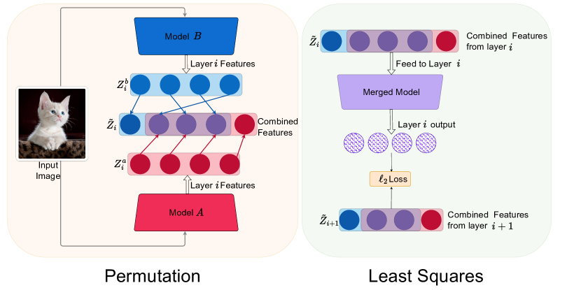
Figure 1: PLeaS is a two-step algorithm for merging models: The first step (left) finds layer-wise Permutations to match features across models to compute combined features $\tilde{Z_{i}}$. Features which are similar are merged, while those which are dis-similar are kept separate. The number of features to be merged depends on the target compute budget, and can be different for each layer. The second step of PLeaS (right) aims to find weights of the merged model which can map the combined features of layer $i$ (i.e., $\tilde{Z}_{i}$) to those of layer $i+1$ (i.e., $\tilde{Z}_{i+1}$) appropriately by solving layer-wise Least Squares problems for each layer.

PLeaS (short for Permutations and Least Squares) is a two-stage algorithm which works with models having the same architecture. The first step consists of matching features across the models. We harness the idea of permutation invariance in neural networks to find an appropriate pairing of features. Inspired by the Git Re-Basin [1] algorithm, which is designed for merging two models that are trained on the same data, we introduce a matching algorithm that finds permutations between similar features across models, while separating dissimilar features in the final merged model. This is critical when merging models trained on widely different tasks, since it prevents interference between features while still merging overlapping features, improving upon prior work such as ZipIt[28], which merges all the neurons of some layers of the two models. This also gives PLeaS fine-grained control over the width of each layer of the merged model. It can hence flexibly trade-off memory/compute and performance according to the deployment requirements.

It has been observed that permutation matching alone suffers from significant performance loss when merging vastly different models, e.g. those trained on disparate data [33]. We hypothesize that while permuted features are powerful when ensembled, simply averaging the permuted weights degrades the features of the merged model. This results in the observed decline in performance.

Hence, in the second step of PLeaS, we solve a layer-wise Least Squares problem, so that each layer of the merged model mimics the permuted ensemble of features from the corresponding layer of the original models. This leads to better representations and superior down-stream performance.

Apart from the target compute budget, PLeaS is hyperparameter free, making it easy for practitioners to use. A schematic of PLeaS is depicted in Fig. 1. We empirically demonstrate that PLeaS can outperform prior work in the challenging setting of merging differently initialized models which have been trained on different datasets.

We merge ResNet models fine-tuned on different datasets in Sections 5.2 and 5.3, and find that PLeaS improves upon the state-of-the-art by 8 to 15% with the same merged model size. Our empirical results are on subsets of DomainNet, and on fine-grained classification tasks. Further, PLeaS, with significantly lower FLOPs, can approach the performance of ensemble methods in some cases (Section 5.5).

The proposed approach can be seamlessly extended to the scenario where data from the fine-tuning domains is unavailable. We call this variant PLeaS-free. This variant uses data from publicly available datasets (like ImageNet) to merge models. We demonstrate in Section 5.4 that PLeaS-free can perform competitively to PLeaS which uses the actual data from the training domains of the component models. This is highly encouraging, as it demonstrates the applicability of PLeaS-free in scenarios where data from the training domains is unavailable due to privacy or commercial reasons.

In summary, our contributions are the following:

• We generalize Git Re-Basin [1] to support partial merging of corresponding layers of two models (Section 4.1) and propose a strategy that automatically selects the target width of each layer of the merged model under a fixed FLOP budget (Section A.2). This gives the practitioner the freedom to choose the size of the final merged model as per resources available at inference. Investigating this tradeoff is one of the goals in this work, e.g., Fig. 3.

• Motivated by the success of ensemble methods, we propose to assign weights to the merged model by solving a least squares problem attempting to mimic ensemble methods at each layer (Section 4.2). Ablation study for this step is in Fig. 3.

• On a test-bed of multiple datasets (with both shared and different label spaces), we showcase that PLeaS outperforms recent merging methods by 8-15 percentage points.(Section 5) at the same model size. Further, PLeaS approaches the ensemble accuracy while using 40% fewer parameters. When no training data is available, PLeaS-free remains competitive to PLeaS (Fig. 4).

2 Related works

There has been growing interest recently in merging models with minimal data and compute overhead. Here, we focus on methods which merge models with the same architecture.

Merging models fine-tuned from the same initialization.

Several methods aim to merge models in the weight space. Ilharco et al. [12] simply add up task vectors, the weight differences of fine-tuned models from the pretrained model, and demonstrate a strong baseline for merging fine-tuned models. Other approaches edit the task vectors based on magnitude of the weights [32, 36] to resolve interference while merging. Some methods aim to find layer-wise [35, 2] or parameter-wise [19] coefficients for merging different task vectors. However, such methods work with task vectors, assuming that the base pretrained model is shared across the fine-tuned models, and hence cannot be easily extended to settings where models are fine-tuned from different starting points. A different line of work [14] proposes layer wise distillation, aiming to minimize the sum of the $\ell_{2}$ distances between the activations of the merged model and the original models. However, naively applying this to models which are vastly different leads to performance degradation, as we show in Section 5. Further, these methods do not provide a way to control the size of the merged model. Although not designed for this scenario of merging fine-tunes of a common pre-trained model, PLeaS  still allows us to achieve significant performance gains when the merged network is slightly larger than the original model (e.g. by 20%) as demonstrated in Table 2.

Merging from two different initializations.

We consider a less restrictive setting, where the models being merged can have different initializations. This has been studied in the literature, and existing works propose weight or activation matching algorithms for this task. Git Re-Basin [1] proposes an algorithm to compute permutation matrices to match the weights of the hidden layers of two or more neural networks. Yamada et al. [33] investigate the usage of permutations to merge models trained on different datasets, however, their study is limited to wide ResNet models on MNIST and CIFAR datasets. These permutation symmetries have also been studied in [20, 33, 5, 27]. Another recent work – ZipIt! [28], tackles a similar problem of merging models finetuned on different datasets from different initializations. ZipIt! proposes an alternative formulation for this task, allowing for feature matching across and within models and puts forth a greedy algorithm to optimize for this. ZipIt! also allows for merging up to some layers of the component models. While this can provide a knob for controlling the size-performance trade-off of the merged model, the empirical performance of their proposed scheme can be improved upon, as we show in Section 5.3. On the other hand, our work describes a merging formulation which is more expressive and allows for partial merges even within layers to minimize feature interference. Finally, He et al. [11] also propose a method to merge networks layer-wise in a progressive manner, which involves light-weight retraining. However, their method requires domain labeled data at both training and inference time, while we require unlabeled data only and also propose a method using no data at all.

Other merging paradigms

Other model merging approaches include mixture of experts [26, 29], selecting experts using test data [18], and sparse expert ensembles [10]. These come with larger compute or memory over-heads, both at inference and training time.

3 Preliminaries

Notations. For simplicity, we describe our method for two $L$-layered MLPs. However, it can be readily extended to convolutional and residual networks, as we demonstrate in our experiments. Let $\Theta^{A}=\{W^{A}_{1},W^{A}_{2},\cdots,W^{A}_{L}\},\Theta^{B}=\{W^{B}_{1},W^{B}_{2},\cdots,W^{B}_{L}\}$ be the parameters of two MLPs $A,B$ having the same architecture. We omit the layer-wise bias here for simplicity. Let $z_{i}^{A},z_{i}^{B}$ denote the input activations to the $i$^th layer of each network respectively, and $d_{i}$ denote the dimension of $z_{i}^{A},z_{i}^{B}$. We also define $Z_{i}^{A},Z_{i}^{B}\in\mathbb{R}^{d_{i}\times n}$ to be the activations of a batch of $n$ inputs. Note that $z_{1}^{A}=z_{1}^{B}=x$, and $z_{L+1}^{A}=y^{A},z_{L+1}^{B}=y^{B}$. Finally, let $\{W_{i}^{M}:i\in\{1,2,\cdots,L\}\}$ be the weights of the merged model. We allow the merged model to have varying widths (which can be different from the widths of the base model), depending on the memory and compute resources available.

Background on Git Re-Basin. Our method is inspired by Git Re-Basin [1], which aims to find permutation matrices $\pi=\{P_{1},P_{2},\cdots,P_{L}\}$ to permute the weights of model $B$. The merged model is formed by permuting and averaging the weights, i.e., $W_{i}^{M}=(1/2)(W_{i}^{A}+P_{i}W_{i}^{B}P_{i-1}^{T})$.

Ainsworth et al. [1] propose a method for computing the permutation matrices by directly optimizing the average similarity between permuted weights of model $B$ and the original weights of model $A$. This weight matching greedily finds a solution to the following sum of bilinear assignment problems,

$$\operatorname*{arg\max}_{\pi=\{P_{i}\}_{i=1}^{L}}\;\;\sum_{i=1}^{L}\;\langle W_{i}^{A},P_{i}W_{i}^{B}P_{i-1}^{T}\rangle\;,$$

where $P_{0}$ is defined to be the identity matrix. This has an advantage of not requiring any data to solve the optimization, but an optimal solution is computationally intractable. Instead, when some samples are available to the optimizer, Ainsworth et al. [1] propose a computationally efficient alternative called activation matching, which solves the following optimization problem:

$$P_{i}\;\in\;\operatorname*{arg\min}_{P\in S_{d_{i}}}\;\|Z_{i}^{A}-PZ_{i}^{B}\|_{F}^{2}\;.$$

Here, $S_{d_{i}}$ refers to the set of permutation matrices of size $d_{i}\times d_{i}$. Computing the activations $Z$’s require samples from the data. However, this optimization can be efficiently solved separately for each layer.

4 Method : PLeaS 

We call our approach to model merging PLeaS. We harness permutation symmetries to match features between two models, inspired by Git Re-Basin[1]. We extend this method to allow for partial merging of models, where each layer can have a different number of merged neurons.

We then compute the weights of the final merged model by solving layer wise least squares problems to ensure that activations of the merged model resemble the permuted activations of the original models.

4.1 Extending Git Re-Basin to partial merging

Note that in Git Re-Basin, two models are averaged (after permuting one model) and hence the dimension of the merged model is the same as the base models. However, when the networks $A,B$ are trained on different datasets, not all features might be compatible across models, and might interfere with each other if merged, leading to degraded performance. Further, those incompatible features might need to be retained in the merged model in order to make accurate predictions on both tasks. Merging all nodes in every layer discounts this possibility, leading to performance degradation, as we show in Fig. 4(b). To this end, we aim to merge features which are similar across the two models, while keeping those which are very different as separate features in the merged model. We hence propose a framework for partially merging model features by leveraging permutations.

Given a permutation matrix $P_{i}$, we select $k_{i}$ indices from $[d_{i}]$ for which the distance between the features of model $A$ and the permuted features of model $B$ for layer $i$ is the smallest. These $k_{i}$ features are merged, while other features are retained separately in the final model.

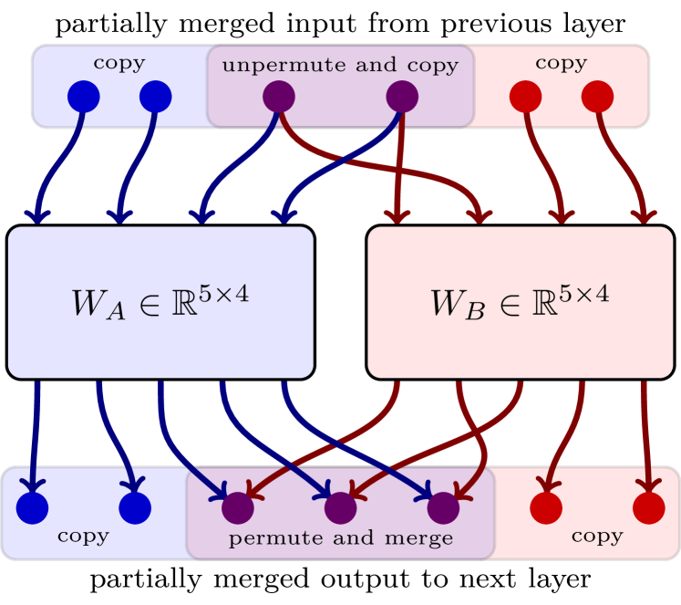
Figure 2: Partial merging with permutations: We show the construction of the $7\times 6$ weight matrix $W_{i}^{m}$ from two weights of size $5\times 4$. The merged inputs are copied and unpermuted to approximate the original inputs. Then we apply both weight matrices separately. Finally, we pair up the merged outputs and average the pairs. Since all operations used are linear, we can fuse them to construct $W_{i}^{m}$ using a single linear layer.

In particular, we find a subset $J_{i}$ satisfying

$$J_{i}\in\operatorname*{arg\min}_{\{J:J\subseteq[d_{i}],|J|=k_{i}\}}||Z_{J,i}^{A}-(P_{i}Z_{:,i}^{B})_{J}||_{F}^{2}.$$

This is simple to implement: retain the indices with the smallest $k_{i}$ distances between the (permuted) activations. For weight matching, we can retain the indices with the largest similarity between the (permuted) weights for each layer. The size of $W_{i}^{M}$ is then increased to $(2d_{i}-k_{i})\times(2d_{i+1}-k_{i+1})$ in exchange for improved performance. This partial merging scheme is illustrated in Fig. 2. Investigating this trade-off between the size and the performance of the merged model is one focus of this paper.

Note that the ratio of ${k_{i}}/{d_{i}}$ can be chosen to be different for each layer. In Section A.2, we introduce a scheme to find such a configuration of these ratios for a given target compute/memory budget $B$; this optimizes a proxy of the downstream performance without using any validation data from the target domain, and is used in all our experiments. The permutation matrices are computed using the weight matching strategy from Git Re-Basin. In Section 5.4, we compare this with using the activation matching strategy, which we call PLeaS-Act .

4.2 Permuted least squares

Suppose, for example, that the target merged model has the same architecture and size as each of the base models. Once the permutations, $P_{i}$’s, have been computed, we propose optimizing the weight matrices of the merged model by solving the following least-squares problem:

$$W_{i}^{M}\;\in\;\operatorname*{arg\min}_{W\in\mathbb{R}^{d_{i}\times d_{i+1}}}\|(Z_{i}^{A}+P_{i}Z_{i}^{B})W-(Z_{i+1}^{A}+P_{i+1}Z_{i+1}^{B})\|^{2}\;,$$ (1)

independently for each layer $i\in[L]$. This is motivated by the impressive performance of the ensemble method (e.g., [33] and Section 5), which retains two separate models and only averages the (permuted) activations at the last layer (before softmax): $\tilde{z}_{L+1}=z^{A}_{L+1}+z^{B}_{L+1}$. We aim to have our merged model approximate such activations. We inductively assume that the first $i-1$ layers are properly merged. Hence, the ensemble of the permuted features (of the $i^{\rm th}$ layer) of the component models can be well approximated by the activations at the input of the $i^{\rm th}$ layer of the merged model. We denote the ensembled features by $\tilde{Z}_{i}=(Z_{i}^{A}+P_{i}Z_{i}^{B})\in{\mathbb{R}}^{d_{i}\times n}$. The goal of the above optimization is to match the ensembled activation of the next layer, $\tilde{Z}_{i+1}=(Z_{i+1}^{A}+P_{i+1}Z_{i+1}^{B})$, with a linear transform of the input ensemble: $\tilde{Z}_{i}W$. We empirically validate this choice of using a permuted ensemble of features to optimize the weights of the merged model in Table 3 in Section B.1, where we compare with alternatives choices to Eq. (1).

This second step of PLeaS is similar to feature distillation. However, the key novelty arises from averaging the permuted features for transferring knowledge from multiple models. This is critical for accurate prediction. In Section 5, we compare PLeaS against RegMean [14], which optimizes an objective similar to Eq. 1 without the permutations and averaging. This method merges models by minimizing $\|Z_{i}^{A}W-Z_{i+1}^{A}\|^{2}+\|Z_{i}^{B}W-Z_{i+1}^{B}\|^{2}$. As we show in Section 5, RegMean performs poorly compared to PLeaS . Apart from the inference computation budget for the final model, PLeaS is completely hyperparameter free.

Note that the second step of PLeaS is fully compatible with the partial merging of Section 4.1 as well: we can directly set the values of $W_{i}^{M}$ corresponding to the unmerged features to be the respective values of $W_{i}^{A}$ and $W_{i}^{B}$. While the objective in Eq. 1 can be minimized in closed form using Ordinary Least Squares (OLS), we practically implement it using gradient descent for ease of use with convolution layers. Given that the objective is convex if computed layer-wise, the weight matrices $W_{i}^{M}$ converge in relatively few steps (less than 100) of gradient descent. Further, we solve this optimization independently for each layer, which can be efficiently parallelized.

4.3 Data requirements of PLeaS 

PLeaS has two steps. The first step finds permutations to match features using weight or activation matching. The second step computes weight matrices to mimic the ensemble of the merged features more closely. In order to compute these features, one could use the data from the training domains, however, this may not be feasible for privacy or commercial reasons. Hence, we propose an alternative scheme—dubbed PLeaS-free —which uses a general vision dataset, like ImageNet, to compute the activations of the component models. These activations are then used to merge domain specific models without requiring any data from their training domains. In Section 5.4, we demonstrate that PLeaS-free suffers minimal degradation compared to PLeaS, suggesting a wider applicability.

5 Experiments

5.1 Settings

We show the effectiveness of our method in merging ResNet-50 models fine-tuned on different datasets starting with different initializations. We consider the following experimental settings:

• Section 5.2 and Section 5.3 deal with the problem of merging models fine-tuned on different datasets with shared or different label spaces respectively.

• Section 5.4 considers the setting where we do not have access to data from the training domains.

• Section 5.5 deals with merging models which were fine-tuned from the same base model.

• Finally, Section B.4 considers a setting where we want to merge differently initialized models trained on the same dataset, and Section B.1 provides an ablation study over the choice of loss functions.

Unless specified otherwise, we use the weight matching strategy from [1] to compute the permutations for PLeaS . For each task, we also report results for Permutations, which is the model obtained by weight averaging the component models after applying the permutations obtained from the first step of PLeaS . Following the recommendation from REPAIR [15], we recompute the batch-norm parameters of the model after merging for all methods. We run each merging experiment for three different seeds, and across two different initial models. We find that inter-run deviation in performance is low, with the standard deviation usually being less than 1%. We report disaggregated results along with these standard deviations in Section B.5.

Baselines

We compare our method against prior works including Git Re-Basin[1], Simple Averaging [12], RegMean [14] and ZipIt! [28]. We also consider two practical upper bounds – training a router model based Mixture of Experts model (MoE), and ensembling the predictions (or activations) of the original models. The former requires storing both models and running one of them based on the router, hence having $1.1\times$ FLOPs and $2\times$ memory requirements, while the latter requires running both the models in parallel, and hence has $2\times$ FLOPs and memory requirements. We find that the performance of the ensemble and MoE models is close to the best performance of a single model on the dataset that it was trained on.

5.2 Models fine-tuned with a shared label space

Table 1: Merging models trained on pairs of different datasets: For each pair of datasets, we merge models and compute the final accuracy on the pair. To compute the final accuracy on a dataset, we average the accuracies across the pairs that it is a part of. We report the accuracies of the merged models for the Same Label Space setting, and a linear probe accuracy on the representations of the merged model for the Different Label Space setting. * Note that here the merged models (bottom five) have the same size as the original, but the MoE and ensemble have a size twice the original.

Method	FLOPs	Size	Same Label Space				Different Label Spaces
			Clip	Info	Paint	Real	CUB	Pets	Dogs	NABird
MoE*	$1.1\times$	$2\times$	69.1	36.1	65.7	78.0	81.1	92.7	83.1	75.8
Ensemble*	$2\times$	$2\times$	63.6	30.3	61.0	74.7	80.5	92.8	82.1	76.1
Simple Avg	$1\times$	$1\times$	1.2	0.8	1.9	2.1	7.1	19.2	9.2	4.7
RegMean[14]	$1\times$	$1\times$	16.6	5.8	10.1	15.8	42.5	45.1	20.2	37.1
ZipIt[28]	$1\times$	$1\times$	26.9	12.2	27.1	37.4	67.5	83.6	60.0	56.3
Git Re-Basin[1]	$1\times$	$1\times$	18.2	7.8	18.8	26.5	66.2	80.2	62.6	59.4
PLeaS (Ours)	$1\times$	$1\times$	41.7	16.9	40.8	55.1	77.3	84.3	69.8	61.8

We fine-tune ImageNet pre-trained ResNet-50 models on four different domains of the DomainNet[23] dataset: Clipart, Infograph, Painting and Real. We merge models trained (from different initializations) on different domains in a pair-wise fashion, and compute the accuracy of the merged model on both the domains. For each domain, we average the performance across all domain pairs. We report this in Table 1 for merged models at $1\times$ size of the original model for different methods.

We also compute the average performance of each algorithm across all datasets at different size/FLOPs budgets, and plot this out in Fig. 3(a).

We find that PLeaS consistently outperforms ZipIt! at various FLOPs budgets. The gains are particularly striking for lower FLOP budgets, where PLeaS outperforms ZipIt! by up to 10%. The power of partial merging is also observed from these results, as one can see that increasing the flops by just 20% leads to massive improvements in the accuracies. Finally, one can see the importance of our layer-wise least squares, since it improves the performance of PLeaS over Permutation by over 20% on average at $1\times$ model size. The gains decrease as we add more capacity to the merged model, which is expected.

5.3 Models with different label spaces

We fine-tune models on CUB[31], NABirds[30], Oxford-IIIT Pets[21] and Stanford Dogs[16] datasets, and merge them upto the penultimate layer. Since the label spaces are different, we aim to evaluate the representations of the penultimate layer of these merged models by training a linear probe on top of the representations. We average the results in the same manner as for DomainNet, and report the performance of different methods for $1\times$ model sizes in Tab 1. We also depict the compute-performance trade-off in Fig 3(b).

In App B.6, we follow the setting of [28], and use task specific heads from the original models to compute the accuracy of the merged model, which requires knowing the domain of the test data point.

Similar to the results on DomainNet, we observe that PLeaS has non-trivial gains over ZipIt! and Git Re-Basin, outperforming ZipIt! by 7% at $1\times$ model size. These results also provide evidence of the effectiveness of our partial permutation scheme — Permutations can outperform ZipIt! at intermediate model budgets by up to 3%. A reason for this could be that the features of the models being merged are sufficiently different, leading to performance degradation if all of them are forced to be merged (a la ZipIt!). Our scheme retains some of these features in the intermediate layers, which could explain the better performance.

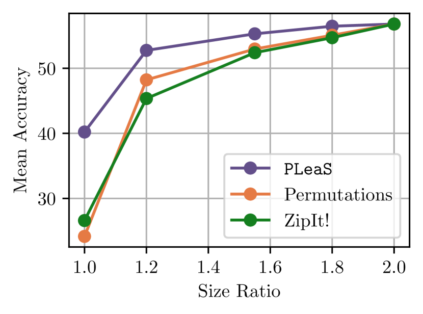
(a) Shared Label Space

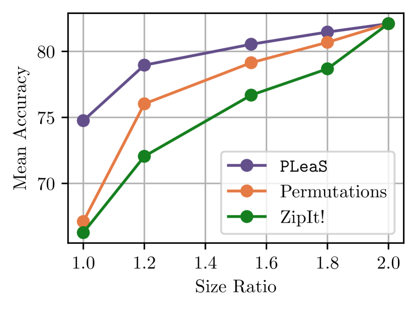
(b) Different Label Spaces

Figure 3: Memory-Performance trade-off for merged models: We merge pairs of models fine-tuned on different datasets, and compute the average performance across all four datasets for two settings - datasets with a Shared label space (Fig. 3(a)), and datasets with Different label spaces (Fig. 3(b)). We plot this average accuracy against the size of the final merged model, and find that PLeaS dominates the state-of-the-art methods.

5.4 Does PLeaS need data from the training domains?

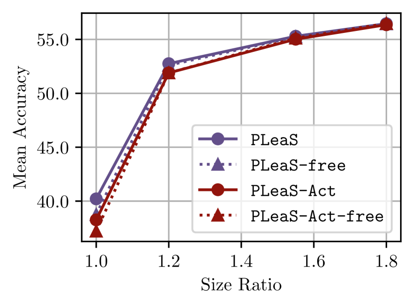
(a) Shared Label Space

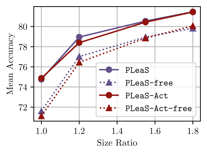
(b) Different Label Spaces

Figure 4: Investigating the data requirement of PLeaS : We run PLeaS-Act and PLeaS using data from the actual domains or ImageNet (indicated by the suffix free) for both the Shared label space (Fig. 4(a)) and Different label spaces (Fig. 4(b)) settings. We plot the average accuracy (or linear probe accuracy) of each variant across all datasets against the relative size of the output model. We find minimal performance drops when using data from ImageNet instead of data from the original training domains.

To investigate the data requirements of our method, we compare the performance of PLeaS and PLeaS-free when merging models trained on different datasets. We also compare the effect of using activation matching to find the permutations for PLeaS , and we term this variant as PLeaS-Act . The performance-model size tradeoff is reported in Figs. 4(a) and 4(b) for the two settings of shared and different label spaces.

We find that PLeaS-free retains a similar performance when using ImageNet instead of the actual domain data for merging models on DomainNet, achieving a drop of less than 1% in accuracy at $1\times$ model size. There is almost no drop at higher sizes of the merged model. We also find that PLeaS slightly outperforms PLeaS-Act , with the difference being around 1% at $1\times$ model size. Notably, even on the more difficult task of merging models with different label spaces, using ImageNet data for computing activations can perform competitively to using the actual data: linear probing on the representations from PLeaS-free performs within 2% of the PLeaS at $1.2\times$ model size, and the gap is less than 4% at $1\times$ model size. This result is particularly encouraging, since it extends the practical applicability of PLeaS-free . Note that while we use data from the actual domains for linear probing, i.e. to assess the quality of the representations, we do not use it for actually merging the models.
We also find that PLeaS-Act performs similarly to PLeaS , with the latter performing better in the shared label space setting. We hypothesise that this is because we use only few batches of data to compute the activations for matching the two network, which leads to deteriorated permutations. However, the difference in performance decreases with increasing model size.

5.5 Merging models with the same initialization

Table 2: Merging models fine-tuned from the same initialization: We merge pairs of models fine-tuned from the same base model and compute the average accuracy across all pairs of domains for each dataset in the Shared Label Setting. We find that PLeaS can approach the performance of the ensemble while having a $1.2\times$ sized merged model.

Method	Size	Clipart	Infograph	Painting	Real
TaskVectors	1.0	58.2	28.9	55.7	70.2
RegMean	1.0	58.9	29.0	57.4	71.8
ZipIt	1.0	54.1	25.2	51.2	66.1
PLeaS	1.0	60.1	29.6	58.0	72.0
PLeaS	1.2	64.2	31.9	61.8	76.0
Ensemble	2.0	64.4	32.0	62.0	76.1

In Tab 2, we evaluate the performance of our method for merging models fine-tuned from the same starting model. We compare against simple average (Task Vectors), ZipIt, and RegMean and find that the performance is similar across methods, with PLeaS being slightly better than the baselines. In fact, task vectors is an effective baseline here. However, we note that 20% extra parameters in the merged model can lead to closing the gap between the ensemble and the merged model produced by PLeaS , demonstrating the need for flexible merging methods.

6 Limitations and future work

The scope of this study is limited to merging models with the same architecture, and applying PLeaS to merge different architectures could be an interesting future direction. Since PLeaS is a two-stage algorithm, its running time is greater than some existing works [28, 12, 14]. However, since the second step can be computed in parallel for all layers, the runtime over-head is small. We further discuss this aspect in Section A.1. Finally, our study of model merging is limited to architectures with convolutions and residual connections, in line with prior work (e.g. [28, 33]). Extending this framework to other architectures such as transformers is another exciting future direction.

7 Conclusion

In this work, we present PLeaS, an algorithm to merge models trained on different datasets starting from different initializations. We demonstrate that PLeaS can effectively produce merged models at different points on the compute-performance trade-off curve. We also propose PLeaS-free, a variant which can merge models without needing any data from the training domains of the component models, and empirically validate that its performance is comparable to running PLeaS with data, which widens its applicability to data-scarce regimes.

Appendix A Experimental and Implementation details

In this section, we provide more details about our experiments. We conduct all experiments using PyTorch [22]. We use two ImageNet pretrained base models for fine-tuning. One of these is the default ResNet50_Weights.IMAGENET1K_V1 from PyTorch, while we pre-train the other starting from random initialization following the same pipeline. For fine-tuning the models on each domain, we use the Adam [17] optimizer, and sweep the learning rates logarithmically between [1e-4,1e-1], testing out 4 values for LR. We validate on the validation subset wherever available, and on 10% of the training dataset where an explicit val set is not provided. We use standard image augmentation techniques. Our MoE model has a light-weight router, which is a 3 layer CNN trained to predict which model to use for classifying an image.

For finding permutation symmetries, we use the official implementation of Git Re-Basin at this url. We also rely on the implementation of ZipIt! for the comparisons in Section 5.

For solving the least squares objective for PLeaS , we use SGD with a batch size of 32, a learning rate of $10^{-3}$. We sample equally from both datasets in each batch for experiments involving data. We run our algorithm for 100 steps, and find that it converges quickly. For PLeaS-Act , we similarly compute the activations on 100 batches of data for matching and finding the optimal permutations. We also reset batch norm parameters using 100 batches of data from the actual domains for all methods.

For evaluations concerning the same label space setting, we ensure that the final model produces a distribution over the output classes. For ZipIt!, we achieve this by ensembling the predictions across multiple task specific heads. PLeaS on the other hand already produces models with the same output dimensions as the original models.

For evaluations on different label spaces, we train a linear probe on the final layer representations for each merged model. We use training data from the target domains to train this linear probe, run Adam with a learning rate of $10^{-3}$, with a batch size of 64 for 50 epochs.

A.1 Compute time and cost

All our experiments (apart from the pretraining and fine-tuning runs to get the original models) are run on a single RTX 2080 Ti GPU. The first step of our method runs in 2 minutes, with the majority of time devoted to computing the activations. This is commensurate with ZipIt! [28] and Git Re-Basin [1] The second step takes around 4 minutes, which is similar to RegMean [14]. We believe that this can be significantly reduced with better dataloading strategies and more efficient implementation, but that is beyond the scope of this paper.

A.2 Computing the layerwise merging ratio

Note that $k_{i}$ can be different for each layer. Given a configuration $K=\{\frac{k_{i}}{d_{i}}:i\in[L]\}$, we can model the FLOPs/memory of the merged model as a quadratic function of $k_{i}$, which we denote as $\text{Footprint}(K)$. For a given relative memory/FLOPs budget $B$, we want to find $K$ s.t. $\text{Footprint}(K)\leq B$ to maximize the accuracy of a model merged with the configuration $K$. We scale everything so that $B=1$ corresponds to the footprint of a single model. This problem is NP-Hard. We propose a relaxation of the problem in order to get an approximate solution. First, we measure the performance of a set of models merged with “leave one out" configurations of $K$, where for each layer $i$, we construct $K_{i}^{0}=\{k_{j}:k_{j}=d_{i}\ \text{if}\ j=i,\ 0\ \text{otherwise}\}$ and $K_{i}^{1}=\{k_{j}:k_{j}=0\ \text{if}\ j=i,\ d_{i}\ \text{otherwise}\}$. $K_{i}^{0}$ corresponds to merging only layer $i$, keeping all other layers unmerged, and $K_{i}^{1}$ corresponds to merging every other layer while keeping $i$ unmerged. We also compute the accuracies of the fully merged model (denoted by $K^{0}$) and the ensemble (denoted by $K^{1}$). Then, we approximate the accuracy of any given $K$ with a linear function as

$$\text{Acc}(K)=\sum_{i=1}^{L}\frac{k_{i}}{d_{i}}((2-B)(\text{Acc}(K^{1})-\text{Acc}(K_{i}^{0}))-(1-B)(\text{Acc}(K_{i}^{0})-\text{Acc}(K^{0})))$$

This approximates the effect of $k_{i}$ on model performance at budget $B$ by linearly interpolating between the performance with fully merging layer $i$ and keeping it separate. We then propose to solve a quadratically constrained linear program to maximize $\text{Acc}(K)$ subject to $\text{Footprint}(K)\leq B$. This program is non-convex however Gurobi [9] is able to solve the program to global optimality in a few seconds. To faithfully compute the performance of the merged model, one would require validation samples from the target domain. However, we empirically observe that using the accuracy of a configuration $K$ on ImageNet is a good proxy for its performance on other merging tasks as well, and we hence use it to compute the layer-wise merging ratio for all our experiments.

Appendix B Additional Results

B.1 What to optimize for Least Squares?

Table 3: Comparing different objectives for PLeaS : We compare the performance of different loss functions for the Least Squares component of PLeaS . We find that Eq. 1 gives the best performance on DomainNet and ImageNet when merging models completely. Here $\tilde{Z_{i}}=0.5(Z_{:,i}^{a}+P_{i}Z_{:,i}^{b})$ and $\tilde{Z}_{i+1}=0.5(Z_{:,i+1}^{a}+P_{i+1}Z_{:,i+1}^{b})$

Optimization Objective	DomainNet	ImageNet
$\begin{aligned} &\|Z_{:,i}^{a}W-\tilde{Z}_{i+1}\|^{2}+\|P_{i}Z_{:,i}^{b}W-\tilde{Z}_{i+1}\|^{2}\end{aligned}$	22.3	45.1
$\begin{aligned} &\|Z_{:,i}^{a}W-(Z_{:,i+1}^{a})\|^{2}+\|P_{i}Z_{:,i}^{b}W-(P_{i+1}Z_{:,i+1}^{b})\|^{2}\end{aligned}$	30.6	53.2
$\begin{aligned} &\|\tilde{Z_{i}}W-Z_{:,i+1}^{a}\|^{2}+\|\tilde{Z_{i}}W-P_{i+1}Z_{:,i+1}^{b}\|^{2}\end{aligned}$	34.3	58.1
$\|\tilde{Z_{i}}W-\tilde{Z}_{i+1}\|^{2}$	40.1	63.1

In Eq. 1, we propose to solve a least squares problem involving the permuted average activations from each layer of the component models. In Table 3, we demonstrate that this choice is not only natural, but also performs better than other alternatives. It is also interesting to note that the second row in the table corresponds to a permuted version of RegMean[14]. This formulation performs better than RegMean, indicating that using permutations is necessary to align features for networks which were differently initialized. Further, row 3 is similar to the objective proposed by [11], but we show that PLeaS outperforms this objective as well.

B.2 Merging models trained on CIFAR and CINIC

In this section, we present results on merging ResNet-18 models trained on CIFAR-10 and CINIC-Im datasets. CINIC-Im is a subset of the CINIC-10 [6] dataset which does not contain any images from CIFAR-10. We follow the same experimental protocol outlined in Section 5 to train two independent models on these datasets from scratch. We then merge the models and report the results for merging models with $1\times$ size of ResNet-18 in Table 4. We make a few surprising observations in this case. We find that randomly permuting the weights of one model and averaging these weights achieves a non-trivial performance, and this is improved by using Git Re-Basin to find the optimal permutation. Using PLeaS further improves this performance.

Table 4: Accuracy while merging models trained on CIFAR and CINIC-Im: We find that random permutations achieve a non-trivial performance, and PLeaS can improve the overall accuracy.

Method	CIFAR	CINIC-Im
Ensemble	94.5	79.1
Random Permutation	55.1	62.7
Git Re-Basin	67.2	68.3
PLeaS	77.4	77.6

B.3 Merging ResNet-18

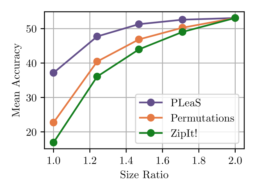
(a) Shared Label Space

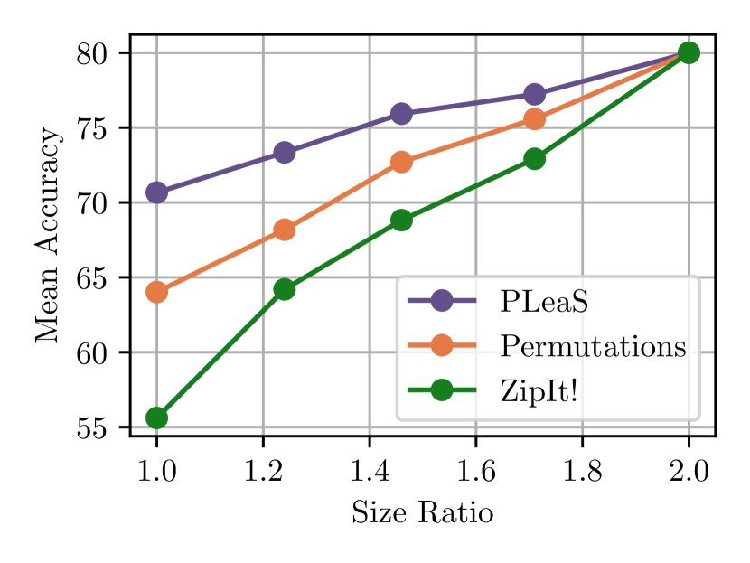
(b) Different Label Spaces

Figure 5: Memory-Performance trade-off for ResNet-18: We merge pairs of models fine-tuned on different datasets, and compute the average performance across all four datasets for two settings - datasets with a Shared label space (Fig. 5(a)), and datasets with Different label spaces (Fig. 5(b))

In Fig. 5, we plot the performance of PLeaS against baselines for merging pairs of ResNet-18 under the same settings as Section 5. We find that PLeaS outperforms the baselines at lower FLOPs, and the difference reduces for larger FLOP budgets.

B.4 Reducing the accuracy barrier on ImageNet

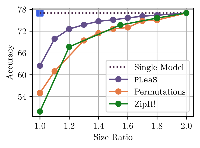
(a) ImageNet performance

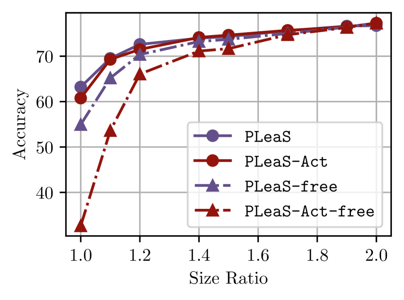
(b) Data-free setting

Figure 6: Merging models trained on ImageNet: In Fig. 6(a), we demonstrate how PLeaS-free can reduce the accuracy barrier by 8% for merging independently trained ImageNet models. This is further reduced for larger target model sizes. In Fig. 6(b), we show the effect of using synthetic data for computing the activations on this task, and find that synthetic data is a viable alternative at larger model sizes.

In this section, we show the performance of PLeaS while merging ResNet-50 models trained independently on ImageNet. The accuracy of a single model on this task is 77.5%. As seen from Fig 6(a), current methods including ZipIt![28] and Git Re-Basin[1] struggle on merging models for this task, with the accuracy of the merged model being significantly lower than the accuracy of a single model. This has been referred to as the accuracy barrier on ImageNet in prior work. PLeaS makes some progress towards lowering this barrier, and improves over Git Re-Basin by over 9% at $1.0\times$ FLOPs budget. For context, this accuracy is at par with that obtained by merging WideResNet-50 models with a width multiplier of 2 using Git Re-Basin. More promisingly, the flexibility afforded by partially permuting and merging models gives another avenue to lower the accuracy barrier, with a model of size $1.4\times$ having an accuracy barrier of 2% with PLeaS . However, further work is needed to reduce this accuracy barrier. In Fig. 6(b), we compare using synthetic data from [3] for all purposes of activation computation while merging ImageNet trained models. We find that using PLeaS-free with synthetic data can come close to using actual data, being within 1% in terms of accuracy at $1.2\times$ model size.

B.5 Detailed Results

Each of our evaluation was run across three random restarts. These random restarts shuffle the data used for computing activations and merging the models. They also affect the initialization of the merged model. Each pair evaluation was also run twice, swapping the order of pre-trained models used for either of the datasets of the pair. We hence have 6 runs for each dataset pair. In Tables 5 and 6, we provide the results for each dataset pair, reporting the average and standard deviation across the 6 runs.

Table 5: Detailed Results on DomainNet

Method	Budget	Data	in-re		cl-pa		cl-in		pa-in		cl-re		pa-re
PLeaS-Act	1.2	Original	26.3 $\pm 1.2$	69.8 $\pm 0.5$	57.3 $\pm 0.7$	53.6 $\pm 0.1$	55.4 $\pm 0.0$	26.6 $\pm 0.0$	52.7 $\pm 0.2$	25.6 $\pm 0.1$	59.1 $\pm 1.3$	69.2 $\pm 1.2$	56.8 $\pm 1.2$	70.3 $\pm 0.9$
PLeaS-Act	1.2	Imagenet	26.6 $\pm 0.9$	69.6 $\pm 0.8$	56.4 $\pm 0.9$	53.9 $\pm 0.2$	55.8 $\pm 0.7$	26.3 $\pm 0.5$	53.3 $\pm 0.2$	25.6 $\pm 0.4$	59.1 $\pm 1.3$	69.3 $\pm 0.9$	56.7 $\pm 1.0$	70.2 $\pm 0.9$
PLeaS-Act	1.0	Original	17.4 $\pm 1.3$	55.0 $\pm 1.5$	40.2 $\pm 2.0$	39.9 $\pm 1.1$	39.5 $\pm 1.5$	17.8 $\pm 0.8$	35.9 $\pm 0.0$	17.3 $\pm 0.0$	42.8 $\pm 2.0$	54.9 $\pm 2.0$	42.3 $\pm 1.7$	56.1 $\pm 1.2$
PLeaS-Act	1.0	Imagenet	17.0 $\pm 1.3$	51.9 $\pm 1.3$	39.7 $\pm 2.4$	38.8 $\pm 0.8$	37.6 $\pm 2.1$	16.6 $\pm 0.7$	37.1 $\pm 1.6$	16.5 $\pm 0.7$	42.2 $\pm 2.9$	53.9 $\pm 1.5$	40.9 $\pm 2.6$	54.4 $\pm 0.9$
PLeaS-Act	1.55	Original	29.0 $\pm 0.8$	72.4 $\pm 0.3$	60.6 $\pm 0.6$	57.3 $\pm 0.0$	59.7 $\pm 0.6$	28.7 $\pm 0.3$	56.4 $\pm 0.1$	27.9 $\pm 0.4$	62.5 $\pm 0.8$	72.3 $\pm 0.9$	60.6 $\pm 1.0$	72.7 $\pm 0.7$
PLeaS-Act	1.55	Imagenet	29.0 $\pm 0.8$	72.5 $\pm 0.6$	60.3 $\pm 0.7$	57.8 $\pm 0.5$	59.9 $\pm 0.6$	29.0 $\pm 0.2$	56.9 $\pm 0.2$	28.1 $\pm 0.3$	62.4 $\pm 0.9$	72.6 $\pm 0.7$	60.1 $\pm 0.9$	72.9 $\pm 0.8$
PLeaS-Act	1.8	Original	29.5 $\pm 0.8$	73.7 $\pm 0.3$	62.3 $\pm 0.5$	59.0 $\pm 0.2$	61.3 $\pm 0.4$	29.8 $\pm 0.2$	58.3 $\pm 0.2$	29.1 $\pm 0.0$	63.7 $\pm 0.6$	73.8 $\pm 0.6$	62.0 $\pm 1.0$	73.9 $\pm 0.7$
PLeaS-Act	1.8	Imagenet	30.1 $\pm 0.8$	73.6 $\pm 0.6$	62.1 $\pm 0.2$	59.9 $\pm 0.4$	61.6 $\pm 0.3$	29.9 $\pm 0.1$	58.4 $\pm 0.2$	28.8 $\pm 0.1$	63.7 $\pm 0.7$	74.0 $\pm 0.7$	61.7 $\pm 0.5$	73.9 $\pm 0.7$
Permutation-Act	1.2	Original	22.3 $\pm 0.9$	62.9 $\pm 1.2$	50.7 $\pm 1.2$	45.9 $\pm 0.2$	48.8 $\pm 0.0$	22.1 $\pm 0.0$	45.4 $\pm 0.4$	21.9 $\pm 0.4$	51.4 $\pm 1.0$	61.6 $\pm 1.7$	49.1 $\pm 1.3$	63.9 $\pm 1.1$
Permutation-Act	1.0	Original	7.6 $\pm 0.2$	24.5 $\pm 1.9$	15.4 $\pm 1.7$	15.5 $\pm 1.8$	15.6 $\pm 0.5$	7.6 $\pm 0.5$	15.4 $\pm 0.9$	6.8 $\pm 0.0$	17.1 $\pm 1.4$	24.6 $\pm 1.7$	18.7 $\pm 0.6$	26.6 $\pm 2.0$
Permutation-Act	1.55	Original	27.1 $\pm 0.7$	69.7 $\pm 0.7$	58.2 $\pm 1.0$	53.6 $\pm 0.4$	56.6 $\pm 0.6$	26.8 $\pm 0.1$	53.3 $\pm 0.4$	25.9 $\pm 0.3$	59.3 $\pm 1.1$	68.8 $\pm 0.8$	57.2 $\pm 0.8$	70.3 $\pm 1.0$
Permutation-Act	1.8	Original	28.9 $\pm 0.8$	71.8 $\pm 0.6$	60.7 $\pm 0.6$	56.8 $\pm 0.3$	59.7 $\pm 0.6$	28.6 $\pm 0.3$	56.5 $\pm 0.4$	27.7 $\pm 0.5$	62.4 $\pm 1.0$	71.4 $\pm 0.8$	60.2 $\pm 0.8$	72.4 $\pm 0.9$
PLeaS-Weight	1.2	Original	27.3 $\pm 1.0$	70.5 $\pm 0.5$	58.8 $\pm 0.2$	54.6 $\pm 0.3$	56.6 $\pm 0.8$	27.2 $\pm 0.3$	53.5 $\pm 0.1$	26.1 $\pm 0.5$	60.9 $\pm 0.2$	68.8 $\pm 0.1$	58.3 $\pm 0.9$	70.5 $\pm 0.8$
PLeaS-Weight	1.2	Imagenet	27.4 $\pm 0.9$	70.2 $\pm 0.6$	57.5 $\pm 0.9$	54.3 $\pm 0.3$	56.9 $\pm 0.4$	27.3 $\pm 0.3$	53.7 $\pm 0.4$	26.0 $\pm 0.6$	59.6 $\pm 1.0$	69.9 $\pm 1.1$	57.6 $\pm 0.8$	70.8 $\pm 0.9$
PLeaS-Weight	1.0	Original	19.2 $\pm 2.0$	56.8 $\pm 1.4$	45.6 $\pm 0.2$	39.9 $\pm 0.2$	41.0 $\pm 1.5$	19.0 $\pm 1.5$	39.6 $\pm 1.3$	17.1 $\pm 0.9$	45.7 $\pm 3.5$	57.3 $\pm 2.1$	43.2 $\pm 2.5$	58.1 $\pm 1.4$
PLeaS-Weight	1.0	Imagenet	17.8 $\pm 1.9$	55.0 $\pm 1.2$	41.0 $\pm 2.9$	40.8 $\pm 1.0$	40.2 $\pm 1.8$	17.9 $\pm 1.2$	38.7 $\pm 1.4$	16.7 $\pm 0.7$	43.7 $\pm 3.7$	56.4 $\pm 1.7$	40.7 $\pm 2.7$	56.1 $\pm 0.7$
PLeaS-Weight	1.55	Original	28.5 $\pm 0.9$	72.9 $\pm 0.4$	61.3 $\pm 0.0$	58.2 $\pm 0.0$	60.0 $\pm 0.4$	29.1 $\pm 0.2$	56.7 $\pm 0.1$	28.1 $\pm 0.2$	63.2 $\pm 0.6$	72.1 $\pm 0.7$	60.4 $\pm 0.8$	73.0 $\pm 0.6$
PLeaS-Weight	1.55	Imagenet	29.1 $\pm 1.1$	72.7 $\pm 0.5$	60.4 $\pm 1.0$	57.4 $\pm 0.6$	60.4 $\pm 0.2$	29.4 $\pm 0.4$	56.9 $\pm 0.3$	28.1 $\pm 0.4$	62.9 $\pm 0.7$	72.2 $\pm 0.8$	60.6 $\pm 0.9$	72.9 $\pm 0.6$
PLeaS-Weight	1.8	Original	29.7 $\pm 1.1$	73.8 $\pm 0.4$	62.7 $\pm 0.2$	59.4 $\pm 0.3$	61.2 $\pm 0.2$	30.1 $\pm 0.2$	58.2 $\pm 0.4$	29.1 $\pm 0.3$	64.1 $\pm 0.5$	73.2 $\pm 0.5$	62.3 $\pm 0.9$	73.8 $\pm 0.7$
PLeaS-Weight	1.8	Imagenet	29.7 $\pm 1.0$	74.0 $\pm 0.5$	62.0 $\pm 0.8$	58.9 $\pm 0.5$	61.5 $\pm 0.1$	30.3 $\pm 0.1$	58.7 $\pm 0.1$	29.1 $\pm 0.1$	63.6 $\pm 0.7$	73.7 $\pm 0.5$	61.7 $\pm 0.6$	74.4 $\pm 0.6$
Permutation-Weight	1.2	Original	24.8 $\pm 1.1$	65.0 $\pm 0.7$	55.0 $\pm 0.0$	48.4 $\pm 0.0$	51.8 $\pm 0.8$	24.0 $\pm 0.3$	48.5 $\pm 0.9$	23.3 $\pm 0.3$	56.3 $\pm 0.3$	63.7 $\pm 0.2$	52.3 $\pm 0.5$	65.5 $\pm 1.1$
Permutation-Weight	1.0	Original	10.5 $\pm 0.7$	34.6 $\pm 2.7$	28.3 $\pm 0.1$	22.9 $\pm 0.1$	21.8 $\pm 1.2$	9.7 $\pm 0.7$	21.1 $\pm 1.9$	9.4 $\pm 0.1$	29.1 $\pm 1.3$	38.1 $\pm 2.9$	26.5 $\pm 1.5$	38.1 $\pm 1.2$
Permutation-Weight	1.55	Original	27.5 $\pm 0.9$	69.7 $\pm 0.7$	59.9 $\pm 0.2$	54.9 $\pm 0.1$	57.7 $\pm 0.8$	27.7 $\pm 0.5$	54.1 $\pm 0.7$	26.3 $\pm 0.2$	60.6 $\pm 0.8$	69.4 $\pm 0.8$	57.4 $\pm 0.9$	70.4 $\pm 0.9$
Permutation-Weight	1.8	Original	28.9 $\pm 0.8$	71.7 $\pm 0.5$	61.6 $\pm 0.1$	57.3 $\pm 0.1$	60.5 $\pm 0.7$	29.0 $\pm 0.3$	56.8 $\pm 0.7$	28.1 $\pm 0.6$	63.1 $\pm 0.9$	71.1 $\pm 0.7$	60.8 $\pm 0.8$	72.2 $\pm 1.0$
ZipIt!	1.2	Original	60.0 $\pm 1.2$	21.9 $\pm 1.1$	52.4 $\pm 1.4$	44.8 $\pm 0.7$	49.8 $\pm 0.3$	21.4 $\pm 0.6$	45.7 $\pm 0.8$	20.6 $\pm 0.2$	54.1 $\pm 2.2$	59.6 $\pm 1.3$	50.3 $\pm 1.3$	63.6 $\pm 0.7$
ZipIt!	1.0	Original	35.8 $\pm 1.3$	13.2 $\pm 0.6$	29.3 $\pm 2.6$	26.1 $\pm 0.5$	26.1 $\pm 1.2$	12.4 $\pm 0.8$	24.4 $\pm 1.2$	10.9 $\pm 0.7$	33.4 $\pm 2.8$	37.0 $\pm 0.5$	31.0 $\pm 1.8$	39.4 $\pm 1.5$
ZipIt!	1.55	Original	66.3 $\pm 0.7$	26.6 $\pm 1.0$	61.2 $\pm 1.0$	53.6 $\pm 0.2$	58.6 $\pm 0.2$	25.9 $\pm 0.3$	52.6 $\pm 0.4$	25.5 $\pm 0.3$	62.9 $\pm 1.1$	67.5 $\pm 0.3$	58.3 $\pm 1.1$	69.9 $\pm 0.2$
ZipIt!	1.8	Original	68.4 $\pm 0.1$	28.7 $\pm 1.2$	63.1 $\pm 0.7$	56.6 $\pm 0.4$	60.8 $\pm 0.3$	27.9 $\pm 0.3$	55.1 $\pm 0.7$	27.3 $\pm 0.2$	65.0 $\pm 0.6$	69.8 $\pm 0.2$	61.0 $\pm 0.9$	72.5 $\pm 0.6$

Table 6: Detailed Results on Different Label Spaces

Method	Budget	Data	na-ox		na-st		cu-na		cu-st		cu-ox		st-ox
PLeaS-Act	1.2	Imagenet	69.2 $\pm 0.2$	88.6 $\pm 0.2$	67.0 $\pm 0.3$	68.6 $\pm 0.5$	78.5 $\pm 0.6$	69.4 $\pm 0.3$	71.9 $\pm 0.5$	71.3 $\pm 0.7$	75.0 $\pm 1.1$	89.4 $\pm 0.7$	77.9 $\pm 0.4$	90.5 $\pm 0.4$
PLeaS-Act	1.2	Original	71.6 $\pm 0.2$	89.5 $\pm 0.2$	70.0 $\pm 0.5$	71.0 $\pm 1.0$	80.1 $\pm 0.5$	72.0 $\pm 0.3$	74.0 $\pm 0.5$	75.2 $\pm 0.6$	76.4 $\pm 0.8$	90.2 $\pm 0.5$	79.9 $\pm 0.5$	91.9 $\pm 0.6$
PLeaS-Act	1.0	Imagenet	66.2 $\pm 0.7$	80.3 $\pm 1.1$	63.6 $\pm 0.8$	56.1 $\pm 0.5$	76.6 $\pm 0.4$	65.4 $\pm 0.6$	67.4 $\pm 1.2$	62.5 $\pm 1.4$	70.9 $\pm 0.6$	84.1 $\pm 1.1$	73.1 $\pm 0.8$	87.4 $\pm 0.3$
PLeaS-Act	1.0	Original	70.2 $\pm 0.2$	81.1 $\pm 0.2$	68.2 $\pm 0.5$	61.2 $\pm 0.6$	79.7 $\pm 0.4$	69.8 $\pm 0.4$	71.5 $\pm 0.7$	69.3 $\pm 1.2$	74.4 $\pm 0.6$	87.2 $\pm 0.5$	78.2 $\pm 0.4$	90.6 $\pm 0.4$
PLeaS-Act	1.8	Imagenet	73.4 $\pm 0.2$	91.6 $\pm 0.2$	71.3 $\pm 0.4$	75.7 $\pm 0.2$	80.2 $\pm 0.3$	72.3 $\pm 0.4$	75.9 $\pm 0.4$	77.4 $\pm 0.3$	77.1 $\pm 1.1$	91.8 $\pm 0.5$	81.3 $\pm 0.3$	92.3 $\pm 0.4$
PLeaS-Act	1.8	Original	75.3 $\pm 0.3$	91.3 $\pm 0.2$	74.0 $\pm 0.6$	76.9 $\pm 0.3$	81.5 $\pm 0.4$	75.0 $\pm 0.3$	77.0 $\pm 0.4$	79.5 $\pm 0.4$	78.8 $\pm 0.5$	92.4 $\pm 0.5$	82.9 $\pm 0.5$	92.8 $\pm 0.4$
PLeaS-Act	1.55	Imagenet	71.5 $\pm 0.3$	90.7 $\pm 1.1$	69.8 $\pm 0.7$	73.7 $\pm 1.1$	79.5 $\pm 0.5$	71.1 $\pm 0.6$	74.9 $\pm 0.3$	75.4 $\pm 0.4$	76.3 $\pm 0.8$	91.2 $\pm 0.5$	80.3 $\pm 0.5$	91.7 $\pm 0.3$
PLeaS-Act	1.55	Original	73.2 $\pm 0.2$	90.4 $\pm 0.2$	72.5 $\pm 0.4$	75.5 $\pm 0.7$	81.2 $\pm 0.6$	73.8 $\pm 0.3$	75.9 $\pm 0.4$	78.3 $\pm 0.6$	78.0 $\pm 0.3$	92.1 $\pm 0.5$	81.9 $\pm 0.4$	92.8 $\pm 0.5$
RegMean	1.0	Original	44.1 $\pm 0.2$	56.0 $\pm 0.2$	51.8 $\pm 14.8$	39.0 $\pm 16.4$	54.1 $\pm 10.1$	42.5 $\pm 13.4$	45.5 $\pm 21.2$	37.7 $\pm 22.3$	55.1 $\pm 20.8$	61.7 $\pm 21.4$	37.4 $\pm 15.5$	56.4 $\pm 16.2$
PLeaS	1.2	Imagenet	71.0 $\pm 0.2$	88.1 $\pm 0.2$	68.5 $\pm 1.0$	70.1 $\pm 0.5$	79.2 $\pm 0.6$	70.4 $\pm 0.3$	73.7 $\pm 1.2$	73.4 $\pm 0.7$	73.5 $\pm 1.8$	89.1 $\pm 0.5$	77.5 $\pm 0.6$	89.9 $\pm 0.3$
PLeaS	1.2	Original	72.5 $\pm 0.2$	88.5 $\pm 0.2$	70.9 $\pm 0.5$	72.5 $\pm 0.5$	80.5 $\pm 0.4$	72.5 $\pm 0.3$	75.2 $\pm 0.8$	76.4 $\pm 0.4$	77.2 $\pm 0.9$	90.7 $\pm 0.6$	79.9 $\pm 0.3$	91.5 $\pm 0.9$
PLeaS	1.0	Imagenet	68.6 $\pm 0.5$	79.4 $\pm 1.0$	66.2 $\pm 0.8$	58.9 $\pm 0.6$	76.5 $\pm 0.6$	65.8 $\pm 1.0$	69.1 $\pm 1.3$	63.9 $\pm 0.7$	71.7 $\pm 1.1$	83.7 $\pm 0.7$	70.9 $\pm 0.4$	84.6 $\pm 0.7$
PLeaS	1.0	Original	70.6 $\pm 0.3$	79.2 $\pm 0.4$	69.6 $\pm 0.6$	62.2 $\pm 0.4$	79.4 $\pm 0.6$	69.8 $\pm 0.4$	72.4 $\pm 0.7$	69.1 $\pm 0.5$	75.2 $\pm 0.8$	87.0 $\pm 0.4$	76.1 $\pm 0.4$	89.4 $\pm 0.5$
PLeaS	1.8	Imagenet	73.4 $\pm 0.6$	91.7 $\pm 0.5$	71.2 $\pm 0.7$	75.8 $\pm 0.5$	80.0 $\pm 0.6$	72.2 $\pm 0.2$	75.5 $\pm 0.8$	77.2 $\pm 0.5$	76.1 $\pm 0.7$	92.0 $\pm 0.7$	80.9 $\pm 0.5$	91.9 $\pm 0.6$
PLeaS	1.8	Original	74.8 $\pm 0.2$	91.6 $\pm 0.2$	73.9 $\pm 0.3$	77.5 $\pm 0.6$	81.7 $\pm 0.4$	74.8 $\pm 0.4$	76.5 $\pm 0.5$	80.2 $\pm 0.3$	78.8 $\pm 0.4$	92.3 $\pm 0.5$	82.8 $\pm 0.5$	92.9 $\pm 0.5$
PLeaS	1.55	Imagenet	72.5 $\pm 0.2$	89.9 $\pm 0.1$	70.1 $\pm 1.0$	74.1 $\pm 0.8$	79.4 $\pm 0.6$	71.6 $\pm 0.3$	74.9 $\pm 0.6$	75.8 $\pm 0.7$	75.8 $\pm 1.1$	91.0 $\pm 0.7$	79.8 $\pm 0.7$	91.4 $\pm 0.5$
PLeaS	1.55	Original	73.9 $\pm 0.4$	90.0 $\pm 0.2$	72.8 $\pm 0.5$	76.0 $\pm 0.6$	81.4 $\pm 0.3$	74.0 $\pm 0.3$	76.1 $\pm 0.5$	78.7 $\pm 0.5$	77.9 $\pm 0.7$	91.9 $\pm 0.4$	81.7 $\pm 0.5$	92.3 $\pm 0.7$
SimpleAvg	1.0	Original	5.2 $\pm 0.9$	21.3 $\pm 1.7$	5.0 $\pm 0.7$	11.2 $\pm 0.9$	8.7 $\pm 0.5$	4.1 $\pm 0.4$	6.8 $\pm 1.0$	9.0 $\pm 0.4$	6.9 $\pm 0.8$	18.0 $\pm 1.2$	8.7 $\pm 0.4$	17.9 $\pm 0.6$
Permutation	1.2	Original	67.9 $\pm 0.7$	87.5 $\pm 0.7$	66.8 $\pm 0.3$	69.6 $\pm 0.4$	78.2 $\pm 0.5$	68.3 $\pm 0.3$	72.0 $\pm 0.8$	72.3 $\pm 0.5$	73.9 $\pm 0.9$	88.9 $\pm 0.3$	77.2 $\pm 0.7$	89.7 $\pm 0.7$
Permutation	1.0	Original	60.6 $\pm 0.4$	78.1 $\pm 0.5$	57.0 $\pm 0.7$	59.1 $\pm 0.5$	72.3 $\pm 0.6$	59.9 $\pm 0.3$	59.8 $\pm 0.8$	60.4 $\pm 0.8$	66.5 $\pm 0.6$	82.1 $\pm 0.8$	67.0 $\pm 0.7$	82.5 $\pm 0.5$
Permutation	1.8	Original	74.0 $\pm 0.6$	91.0 $\pm 0.7$	73.0 $\pm 0.4$	76.3 $\pm 0.5$	81.2 $\pm 0.3$	73.8 $\pm 0.2$	76.0 $\pm 0.5$	78.5 $\pm 0.5$	77.7 $\pm 0.6$	92.1 $\pm 0.6$	82.2 $\pm 0.4$	92.5 $\pm 1.0$
Permutation	1.55	Original	71.4 $\pm 0.6$	90.4 $\pm 0.5$	71.1 $\pm 0.4$	73.9 $\pm 0.5$	80.1 $\pm 0.5$	71.9 $\pm 0.3$	75.0 $\pm 0.7$	76.2 $\pm 0.4$	76.5 $\pm 0.9$	91.0 $\pm 0.5$	80.4 $\pm 0.3$	91.9 $\pm 0.5$
Permutation-Act	1.2	Original	67.1 $\pm 0.6$	85.7 $\pm 0.6$	64.6 $\pm 0.7$	65.3 $\pm 0.9$	77.4 $\pm 0.4$	67.0 $\pm 0.5$	70.2 $\pm 0.9$	69.4 $\pm 0.8$	73.0 $\pm 0.7$	87.7 $\pm 0.4$	76.7 $\pm 0.5$	89.8 $\pm 0.4$
Permutation-Act	1.0	Original	61.2 $\pm 0.7$	75.9 $\pm 1.1$	55.8 $\pm 0.7$	54.8 $\pm 0.9$	73.9 $\pm 0.4$	61.2 $\pm 0.7$	60.9 $\pm 0.8$	59.4 $\pm 1.3$	66.6 $\pm 2.7$	80.0 $\pm 2.2$	71.6 $\pm 0.5$	86.4 $\pm 0.6$
Permutation-Act	1.8	Original	74.1 $\pm 0.4$	91.2 $\pm 0.5$	73.0 $\pm 0.5$	76.1 $\pm 0.8$	81.0 $\pm 0.3$	73.9 $\pm 0.4$	76.4 $\pm 0.4$	78.6 $\pm 0.5$	78.5 $\pm 0.4$	92.1 $\pm 0.6$	82.4 $\pm 0.4$	93.0 $\pm 0.4$
Permutation-Act	1.55	Original	71.6 $\pm 0.4$	89.6 $\pm 0.5$	70.4 $\pm 0.3$	72.4 $\pm 0.9$	79.7 $\pm 0.4$	71.5 $\pm 0.2$	74.4 $\pm 0.5$	75.5 $\pm 0.5$	76.3 $\pm 0.5$	90.9 $\pm 0.4$	80.9 $\pm 0.5$	92.3 $\pm 0.6$
ZipIt!	1.2	Original	62.6 $\pm 0.4$	85.0 $\pm 0.6$	62.0 $\pm 0.9$	63.1 $\pm 0.8$	74.9 $\pm 0.7$	63.6 $\pm 0.7$	70.3 $\pm 0.7$	66.5 $\pm 0.4$	71.1 $\pm 0.9$	85.1 $\pm 0.6$	72.2 $\pm 0.5$	88.2 $\pm 0.3$
ZipIt!	1.0	Original	56.7 $\pm 0.6$	76.7 $\pm 1.3$	55.1 $\pm 0.6$	52.3 $\pm 1.1$	72.9 $\pm 0.4$	57.8 $\pm 0.4$	64.6 $\pm 0.6$	58.3 $\pm 0.9$	67.1 $\pm 0.6$	80.8 $\pm 0.3$	67.6 $\pm 1.3$	85.5 $\pm 0.9$
ZipIt!	1.8	Original	70.0 $\pm 0.4$	91.0 $\pm 0.4$	69.4 $\pm 0.8$	75.0 $\pm 0.7$	78.9 $\pm 0.6$	70.4 $\pm 0.5$	75.7 $\pm 0.4$	76.0 $\pm 0.5$	75.9 $\pm 0.7$	91.0 $\pm 0.5$	78.7 $\pm 0.6$	92.2 $\pm 0.6$
ZipIt!	1.55	Original	67.0 $\pm 0.4$	90.0 $\pm 0.7$	66.4 $\pm 0.3$	72.9 $\pm 0.5$	77.7 $\pm 0.4$	67.3 $\pm 0.8$	73.7 $\pm 0.6$	73.2 $\pm 0.5$	74.0 $\pm 0.5$	89.9 $\pm 0.6$	76.6 $\pm 0.7$	91.4 $\pm 0.5$

B.6 Using task specific heads

Table 7: Evaluating merged models with task specific heads: For each pair of datasets, we merge models and compute the final accuracy on the pair. To compute the final accuracy on a dataset, we average the accuracies across the pairs that it is a part of. These accuracies are computed by using the task specific head for each pair of models.

Method	FLOPs	CUB	NABird	Dogs	Pets
ZipIt[28]	1.0	47.8	46.3	35.7	68.6
Git Re-Basin[1]	1.0	35.3	32.7	26.1	50.4
PLeaS	1.0	63.1	63.2	45.3	68.4
ZipIt	1.2	68.7	64.1	60.9	84.8
Permutation	1.2	65.8	61.7	60.9	83.7
PLeaS	1.2	71.6	69.6	70.2	86.9
ZipIt	1.55	72.9	69.2	71.9	89.7
Permutation	1.55	71.8	68.8	70.1	88.2
PLeaS	1.55	74.5	72.4	74.8	89.8
ZipIt	1.8	75.1	72.7	74.0	91.6
Permutation	1.8	74.1	72.6	75.8	89.9
PLeaS	1.8	77.0	74.3	73.5	89.6
Ensemble	2.0	77.0	76.0	80.8	91.6

In Table 7, we report the results computed using the protocol mentioned in [28]. We find that PLeaS outperforms ZipIt! in this evaluation across model budgets.

Appendix C Broader Impact

Advances in model merging, especially through methods which do not require training data, can help further democratize machine learning by helping practitioners improve the capabilities of open source models. However, the risk of merged models inheriting biases of the component models still remains.

References

- Ainsworth et al. [2022] S. Ainsworth, J. Hayase, and S. Srinivasa. Git re-basin: Merging models modulo permutation symmetries. In The Eleventh International Conference on Learning Representations, 2022.
- Akiba et al. [2024] T. Akiba, M. Shing, Y. Tang, Q. Sun, and D. Ha. Evolutionary optimization of model merging recipes, 2024. arXiv preprint: 2403.13187.
- Baradad et al. [2022] M. Baradad, C.-F. Chen, J. Wulff, T. Wang, R. Feris, A. Torralba, and P. Isola. Procedural image programs for representation learning. In A. H. Oh, A. Agarwal, D. Belgrave, and K. Cho, editors, Advances in Neural Information Processing Systems, 2022.
- Chiang et al. [2023] W.-L. Chiang, Z. Li, Z. Lin, Y. Sheng, Z. Wu, H. Zhang, L. Zheng, S. Zhuang, Y. Zhuang, J. E. Gonzalez, I. Stoica, and E. P. Xing. Vicuna: An open-source chatbot impressing GPT-4 with 90% ChatGPT quality, March 2023. URL https://lmsys.org/blog/2023-03-30-vicuna/.
- Cho et al. [2024] D. K. Cho, J. Yang, J. Seo, S. Bae, D. Kang, S. Park, H. Choe, and W. Lim. ShERPA: Leveraging neuron alignment for knowledge-preserving fine-tuning. In ICLR 2024 Workshop on Mathematical and Empirical Understanding of Foundation Models, 2024. URL https://openreview.net/forum?id=BqIxUKqrdD.
- Darlow et al. [2018] L. N. Darlow, E. J. Crowley, A. Antoniou, and A. J. Storkey. Cinic-10 is not imagenet or cifar-10, 2018.
- Demircan [2022] M. Demircan. The dma and the gdpr: Making sense of data accumulation, cross-use and data sharing provisions. In IFIP International Summer School on Privacy and Identity Management, pages 148–164. Springer, 2022.
- Ganaie et al. [2022] M. Ganaie, M. Hu, A. Malik, M. Tanveer, and P. Suganthan. Ensemble deep learning: A review. Engineering Applications of Artificial Intelligence, 115:105151, Oct. 2022.
- Gurobi Optimization, LLC [2023] Gurobi Optimization, LLC. Gurobi Optimizer Reference Manual, 2023. URL https://www.gurobi.com.
- Gururangan et al. [2023] S. Gururangan, M. Li, M. Lewis, W. Shi, T. Althoff, N. A. Smith, and L. Zettlemoyer. Scaling expert language models with unsupervised domain discovery. arXiv preprint arXiv:2303.14177, 2023.
- He et al. [2018] X. He, Z. Zhou, and L. Thiele. Multi-task zipping via layer-wise neuron sharing. In S. Bengio, H. Wallach, H. Larochelle, K. Grauman, N. Cesa-Bianchi, and R. Garnett, editors, Advances in Neural Information Processing Systems, volume 31. Curran Associates, Inc., 2018. URL https://proceedings.neurips.cc/paper_files/paper/2018/file/ad8e88c0f76fa4fc8e5474384142a00a-Paper.pdf.
- Ilharco et al. [2023] G. Ilharco, M. T. Ribeiro, M. Wortsman, S. Gururangan, L. Schmidt, H. Hajishirzi, and A. Farhadi. Editing models with task arithmetic. In The Eleventh International Conference on Learning Representations, 2023.
- Jain et al. [2023] Y. Jain, H. Behl, Z. Kira, and V. Vineet. Damex: Dataset-aware mixture-of-experts for visual understanding of mixture-of-datasets. In Advances in Neural Information Processing Systems, volume 36, 2023.
- Jin et al. [2023] X. Jin, X. Ren, D. Preotiuc-Pietro, and P. Cheng. Dataless knowledge fusion by merging weights of language models. In The Eleventh International Conference on Learning Representations, 2023.
- Jordan et al. [2023] K. Jordan, H. Sedghi, O. Saukh, R. Entezari, and B. Neyshabur. Repair: Renormalizing permuted activations for interpolation repair, 2023.
- Khosla et al. [2011] A. Khosla, N. Jayadevaprakash, B. Yao, and L. Fei-Fei. Novel dataset for fine-grained image categorization. In First Workshop on Fine-Grained Visual Categorization, IEEE Conference on Computer Vision and Pattern Recognition, Colorado Springs, CO, June 2011.
- Kingma and Ba [2017] D. P. Kingma and J. Ba. Adam: A method for stochastic optimization, 2017.
- Li et al. [2022] M. Li, S. Gururangan, T. Dettmers, M. Lewis, T. Althoff, N. A. Smith, and L. Zettlemoyer. Branch-train-merge: Embarrassingly parallel training of expert language models. arXiv preprint arXiv:2208.03306, 2022.
- Matena and Raffel [2022] M. Matena and C. Raffel. Merging models with fisher-weighted averaging, 2022.
- Navon et al. [2023] A. Navon, A. Shamsian, E. Fetaya, G. Chechik, N. Dym, and H. Maron. Equivariant deep weight space alignment. arXiv preprint arXiv:2310.13397, 2023.
- Parkhi et al. [2012] O. M. Parkhi, A. Vedaldi, A. Zisserman, and C. V. Jawahar. Cats and dogs. In IEEE Conference on Computer Vision and Pattern Recognition, 2012.
- Paszke et al. [2019] A. Paszke, S. Gross, F. Massa, A. Lerer, J. Bradbury, G. Chanan, T. Killeen, Z. Lin, N. Gimelshein, L. Antiga, A. Desmaison, A. Köpf, E. Yang, Z. DeVito, M. Raison, A. Tejani, S. Chilamkurthy, B. Steiner, L. Fang, J. Bai, and S. Chintala. Pytorch: An imperative style, high-performance deep learning library, 2019.
- Peng et al. [2019] X. Peng, Q. Bai, X. Xia, Z. Huang, K. Saenko, and B. Wang. Moment matching for multi-source domain adaptation. In Proceedings of the IEEE International Conference on Computer Vision, pages 1406–1415, 2019.
- Rao et al. [2020] Y. Rao, J. Steeves, A. Shaabana, D. Attevelt, and M. McAteer. Bittensor: A peer-to-peer intelligence market. arXiv preprint arXiv:2003.03917, 2020.
- Roziere et al. [2023] B. Roziere, J. Gehring, F. Gloeckle, S. Sootla, I. Gat, X. E. Tan, Y. Adi, J. Liu, T. Remez, J. Rapin, et al. Code llama: Open foundation models for code. arXiv preprint arXiv:2308.12950, 2023.
- Shazeer et al. [2017] N. Shazeer, A. Mirhoseini, K. Maziarz, A. Davis, Q. Le, G. Hinton, and J. Dean. Outrageously large neural networks: The sparsely-gated mixture-of-experts layer. arXiv preprint arXiv:1701.06538, 2017.
- Singh and Jaggi [2020] S. P. Singh and M. Jaggi. Model fusion via optimal transport. Advances in Neural Information Processing Systems, 33:22045–22055, 2020.
- Stoica et al. [2024] G. Stoica, D. Bolya, J. B. Bjorner, P. Ramesh, T. Hearn, and J. Hoffman. Zipit! merging models from different tasks without training. In The Twelfth International Conference on Learning Representations, 2024.
- Sukhbaatar et al. [2024] S. Sukhbaatar, O. Golovneva, V. Sharma, H. Xu, X. V. Lin, B. Rozière, J. Kahn, D. Li, W.-t. Yih, J. Weston, et al. Branch-train-mix: Mixing expert llms into a mixture-of-experts llm. arXiv preprint arXiv:2403.07816, 2024.
- Van Horn et al. [2015] G. Van Horn, S. Branson, R. Farrell, S. Haber, J. Barry, P. Ipeirotis, P. Perona, and S. Belongie. Building a bird recognition app and large scale dataset with citizen scientists: The fine print in fine-grained dataset collection. In Proceedings of the IEEE conference on computer vision and pattern recognition, pages 595–604, 2015.
- Wah et al. [2011] C. Wah, S. Branson, P. Welinder, P. Perona, and S. Belongie. The caltech-ucsd birds-200-2011 dataset. Technical Report CNS-TR-2011-001, California Institute of Technology, 2011.
- Yadav et al. [2023] P. Yadav, D. Tam, L. Choshen, C. Raffel, and M. Bansal. Ties-merging: Resolving interference when merging models. In Advances in Neural Information Processing Systems, volume 36, 2023.
- Yamada et al. [2023] M. Yamada, T. Yamashita, S. Yamaguchi, and D. Chijiwa. Revisiting permutation symmetry for merging models between different datasets. arXiv preprint arXiv:2306.05641, 2023.
- Yang et al. [2024a] E. Yang, L. Shen, Z. Wang, G. Guo, X. Chen, X. Wang, and D. Tao. Representation surgery for multi-task model merging. arXiv preprint arXiv:2402.02705, 2024a.
- Yang et al. [2024b] E. Yang, Z. Wang, L. Shen, S. Liu, G. Guo, X. Wang, and D. Tao. Adamerging: Adaptive model merging for multi-task learning. In The Twelfth International Conference on Learning Representations, 2024b.
- Yu et al. [2024] L. Yu, B. Yu, H. Yu, F. Huang, and Y. Li. Language models are super mario: Absorbing abilities from homologous models as a free lunch. arXiv preprint arXiv:2311.03099, 2024.