Relativistic Linear Response in Quantum-Electrodynamical Density Functional Theory
Abstract
We present the theoretical derivation and numerical implementation of the linear response equations for relativistic quantum electrodynamical density functional theory (QEDFT). In contrast to previous works based on the Pauli–Fierz Hamiltonian, our approach describes electrons interacting with photonic cavity modes at the four-component Dirac-Kohn-Sham level, derived from fully relativistic QED through a series of established approximations. Moreover, we show that a new type of spin–orbit-like (SO) cavity-mediated interaction appears under the relativistic description of the coupling of matter with quantized cavity modes. Benchmark calculations performed for atoms of group 12 elements (Zn, Cd, Hg) demonstrate how a relativistic treatment enables the description of exciton polaritons which arise from the hybridization of formally forbidden singlet–triplet transitions with cavity modes. For atoms in cavities tuned on resonance with a singlet–triplet transition we discover a significant interplay between SO effects and coupling to an off-resonant intense singlet-singlet transition. This dynamic relationship highlights the crucial role of ab initio approaches in understanding cavity quantum electrodynamics. Finally, using the mercury porphyrin complex as an example, we show that relativistic linear response QEDFT provides computationally feasible first-principles calculations of polaritonic states in large heavy element-containing molecules of chemical interest.
I Introduction
The strength of light–matter coupling, normally weak when a material interacts with vacuum modes of free space, can be greatly enhanced by placing the material into an optical cavity. If a cavity mode is in resonance with an excitation of the material, new hybrid light–matter states called polaritons emerge. [1, 2, 3, 4] Depending on the nature of the excitation, different types of polaritonic states exist such exciton–polaritons and vibrational polaritons resulting from the coupling of light to electronic and vibrational transitions, respectively. As a result a new field of cavity quantum electrodynamical (QED) materials [5, 1, 2, 6, 7] has emerged bringing together various platforms for manipulating and engineering quantum materials with electromagnetic fields. It encompasses a wide spectrum of different fields including quantum optics [8], polaritonic chemistry [1, 9, 2, 10, 11, 12, 13, 7], the generation of light-induced states of matter through classical fields [14, 15] or quantum fields emanating from a cavity [16, 17, 18, 19]. This rapidly growing field has attracted significant attention from both theorists and experimentalists, leading to the exploration of various effects under strong light–matter coupling. Strong light–matter interaction in a cavity enables the modification of chemical reaction landscapes [20, 21, 22, 23, 24, 25] and ground states of matter [26, 27, 28, 29], enhances charge and energy transfer [30, 31, 32, 33, 34, 35], and allows for selective manipulation of electronic states [35], the modification of electron–phonon coupling and superconductivity [36, 37, 38, 39], controlling of excitons [40, 41, 42] while achieving exciton-polariton condensation [43, 44]. In recent studies, Quantum Hall systems, whether operating in the integer regime [45, 46, 47, 48, 49] or the fractional regime [50, 51], have exhibited remarkable phenomena when confined within optical cavities. These systems have shown what is known as ultra-strong coupling with the light field, resulting in significant changes in their transport properties [52]. Furthermore, there is a growing interest in exploring the implications of coupling with chiral electromagnetic fields, and this topic is currently being actively investigated [53, 54, 55, 56]. This regime of the strong coupling between matter and light can be achieved due to collective effects, when a large number of molecules is placed in a cavity and coherently interact with its modes, or for micro- and nano-cavities that confine light to very small length scales [1, 57, 58, 3, 7].
To describe the interaction of the material with vacuum fluctuations i.e. cavity modes, the quantum description of light is important making QED the theory of choice. The standard practical approach is provided by models of cavity QED, which describe a system of photons strongly coupled to a material approximated as a few-level system, e.g. the Jaynes–Cummings [59] and the Dicke [60] model. However, if we want to capture subtle and complex changes of the material inside a cavity, a first principles description of the matter subsystem becomes necessary. [2].
To bridge the worlds of quantum chemistry and quantum optics, new computational methods that simultaneously allow ab initio description of matter while treating transverse photons as dynamical variables, were developed [2, 12, 61, 7]. The first such method was quantum electrodynamical density functional theory (QEDFT) proposed for time-dependent [62, 63, 64] and ground-state/coupled-vacuum properties [65, 66]. Besides non-interacting auxiliary systems in the Kohn-Sham formulation of QEDFT also alternative, explicitly correlated approaches were introduced [67]. The first computational implementations of QEDFT were reported by Flick et al. for time-dependent situations [5, 68], for ground-state properties [26] and finally as a linear response theory of coupled matter–photon system and formulated on a real-space grid. [69] It motivated subsequent implementations based on Gaussian orbitals [70, 71] as well as a development of a real-space Sternheimer formalism [72]. Moreover, the work of Yang et al. [70] also considers various simplified cases based on the neglect of the dipole self-energy terms, on the Tamm–Dancoff approximation (TDA) for electrons [73] as well as on an analogous approximation for photons, together with the different combinations of these approximations. In addition to QEDFT, ab initio theories combining QED with wave function based quantum chemical methods were developed starting with quantum electrodynamical Hartree–Fock (QED-HF) theory [74, 75, 76], and ranging to quantum electrodynamical coupled clusters (QED-CC) [75, 77] and quantum electrodynamical configuration interaction singles (QED-CIS) [78], as well as Green function-based approaches [79] and reduced density-matrix theories [74, 76].
Most of these realizations of QEDFT were based on the non-relativistic Pauli–Fierz Hamiltonian. However, there exists a plethora of phenomena called relativistic effects that are not covered by the non-relativistic, Schrödinger or Pauli equation-based treatment and are described correctly only within relativistic theories based on the Dirac equation. [80] The most prominent examples include the color of gold [81, 82], the liquid state of mercury [83], and the voltage of the lead–acid battery [84]. Further manifestations of relativistic effects in atomic, molecular, and solid state systems involve bound-electron factor [85, 86], electron absorption and X-ray spectra [87, 88, 89, 90, 91], NMR [92, 93, 94, 95], pNMR [96, 97, 98, 99, 100] and EPR spectroscopies [101, 102, 103, 104, 105, 100], bond lengths, [106] reaction mechanisms [107], phosphorescence and decay pathways [108], properties of superheavy elements [109, 110], band structures [111], band gap opening, [112, 113, 114] and the stability of structural phases [115]. Relativistic quantum chemistry [116, 117] addresses the relativistic effects by describing electrons at the level of the Dirac equation. The gold standard is represented by the four-component (4c) Dirac–Coulomb Hamiltonian that combines the one-electron Dirac equation with the instantaneous Coulomb interaction among electrons and nuclei and electrons with each other. [118] This Hamiltonian contains relativistic kinetic energy as well as one-electron spin–orbit coupling and is sometimes extended to include Breit terms. [118, 119, 120, 121] Moreover, there is an ongoing research effort focused on including the effects of relativistic QED in quantum chemistry to account for radiative corrections [122, 123, 124, 125, 126, 127, 128, 129]. At the same time, researchers are developing approximate two-component Hamiltonians that would capture the most important relativistic effects at a lower computational cost. [130, 131, 132, 133]
QEDFT with relativistic Dirac equation-based treatment of electronic structure thus enables the correct description of molecules containing any element across the periodic table when strongly coupled to cavity modes (under certain stability conditions detailed in Sec. II.2). Moreover, the 4c description includes SOC variationally thus allowing first-principles access to singlet–triplet transitions that are forbidden according to non-relativistic theories. While spin–orbit coupling can be added perturbatively, usually up to the first order in ( being the atomic number and the speed of light), the fully relativistic treatment accounts for the higher order effect that can become prominent for high- systems. [134] In addition, the linear response properties such as the coupling strengths between the singlet and triplet states or the phosphorescence parameters are correctly obtained from the first-order perturbation theory [135] instead of requiring the more demanding quadratic response as they would with perturbative SOC. [136] Another case for relativistic QEDFT is provided by cavity engineering of the energy ratio between singlet–singlet and singlet–triplet excited states. This was suggested to improve the yields of singlet fission [137] and intersystem crossing [35, 138], particularly for heavy element-containing systems where the rate of these processes is enhanced by the increased spin–orbit coupling. [139, 140] Additionally, the inclusion of SOC in QEDFT theory will enable to compute spin–orbit related phenomena in complex nanostructures and solids. [141, 142]
At the same time, relativistic QEDFT calculations close the gap between the stable and non-perturbative low-energy sector of QED described by the Pauli–Fierz quantum field theory [143, 144, 7] and a fully second-quantized QED formulation in various flavours [145, 146, 147]. Even without cavities and their changes in the modes of the electromagentic field, there are many fundamental questions still to be answered within QED as a general framework to describe on the most fundamental level the interaction between charged particles and light. [148]
In this work, we introduce a relativistic quantum-electrodynamical density functional theory (QEDFT) for molecules that combines four-component Dirac–Kohn–Sham treatment of electrons with quantized description of photonic modes. We first present the theoretical foundation of the developed method where we derive the relativistic Hamiltonian for the coupled light–matter system in the long-wavelength approximation. We demonstrate the emergence of a novel spin-orbit-like cavity-mediated interaction within the framework of relativistic coupling between matter and quantized cavity modes. Then in Sec. II.4 we formulate a linear response equation in the framework of QEDFT for its excitation energies that allows the first-principles calculation of polaritonically modified spectra and present its numerical implementation. As an example, we calculate the absorption spectra of Zn, Cd, and Hg atoms focusing on the singlet–triplet transitions in a cavity. Via careful analysis of the absorption spectra we show that there is a significant interplay between spin-orbit effects and off-resonant coupling to the intense singlet-singlet transition. This interplay highlights the crucial role of the ab initio approach in understanding cavity quantum electrodynamics. Finally, we considered a large heavy element complex to demonstrate the applicability of our method to systems of chemical interest.
II Theory
The SI system of units is used throughout the paper unless specified otherwise. For additional notations and conventions see Appendix A.
II.1 Light-matter coupling in fully-relativistic limit: total Hamiltonian of a system
We consider a system of electrons minimally coupled to photons in the presence of external classical fields. The full QED Hamiltonian of such a system in Coulomb gauge is formally given as [149, 63]
| (1) | ||||
Here is the speed of the light in free-space vacuum, is the reduced Planck constant, is the vacuum permittivity, is the bare mass of the electron, are the Dirac matrices in the standard representation (see Appendix A). Here all the operators are in the Schrödinger picture and denotes their normal ordering.
The electron-positron field operator is given by [150, 149]
| (2) | ||||
where is an annihilation operator of the electron with momentum and helicity , operator is a creation operator for the positron with the same momenta and helicity. Here and are the solutions of the free Dirac equation for the electron and positron, respectively. The electron-positron field operator formally obeys the usual Heisenberg equation of motion (here we indicate with label the Heisenberg picture)
| (3) |
The Dirac four-current operator is constructed as with the components having the following form
| (4) | ||||
| (5) |
where .
The quantized vector potential in Coulomb gauge is given by [149] 111We note that in comparison with the usual definition of a vector potential, we here have an extra multiplication by in order to have the units of in Volts.
| (6) |
where and are the creation and annihilation operators of a photon with momentum and helicity , respectively; is the energy of the photon and is the transverse dimensionless polarization vector that obeys [149]
| (7) |
We note that in a Coulomb gauge the field is fully transverse, i. e. .
The vector potential formally obeys the following equation of motion
| (8) |
The last term in Eq. (1) is the free photon Hamiltonian which creates and annihilates only transverse photons. Using Eq. (6) one can rewrite it as
| (9) |
Here with the subindex S denoting the Schrödinger picture, and , are quantized transverse electric and magnetic fields, respectively [149], that expressed via photonic creation and annihilation operators assume the form
| (10) | ||||
| (11) |
In our system, we also introduce external (with respect to the system’s electrons plus photons) classical magnetic vector potential and scalar potential as well as classical external four-currents with being a charge density. Using Eq. (6) one can rewrite the energy due to coupling to a classical external charge current as [65]
| (12) |
with the expansion coefficients . We note, that with these expansion coefficients, one can recover the transverse part of the external current since is a transverse vector
| (13) |
II.2 Approximations
We note that so far, we have chosen implicitly circularly polarised vectors . However, for the quantization of the electromagnetic field, one can choose any pair of polarization vectors obeying (7), for example, linearly polarised ones. We also note that circular and linear representations are connected by a canonical transformation that preserves the form of the equations. Therefore, without loss of generality, we restrict ourselves to the case of linear polarisation, i.e., real transverse polarization vectors. Then the coupling term from Eq. (12) reads as
| (14) |
with the real expansion coefficients
| (15) |
Next, we would like to work with a stable vacuum, i.e. the energy gap between the positive and negative energy solutions of the Dirac equation is nonzero. If the intensity of the external fields is small compared to the Schwinger limit, and if one considers the long-wavelength approximation then no pair production occurs [151, 152, 153]. The energy gap then substitutes the boundedness-from-below (minimal-energy state) of non-relativistic theories. Since no pair creation is present, in addition to charge conservation, particle-number conservation is satisfied, allowing us to proceed to a first-quantized formulation for electrons. Specifically due to the long-wavelength approximation, Eq. (6) can be written as
| (16) |
and then the Hamiltonian of Eq. (1) takes a form
| (17) | ||||
where is the number of electrons in the system. Assume we are dealing with a cavity, in which case the free-space mode expansion (16) can be converted into the corresponding expansion for the photonic structure e. g. Fabry–Pérot cavity [154]. Since we are working in a dipole approximation, i.e. no momentum is transferred in a cavity, the actual spatial mode structure and the momentum matching are no longer important. As a result, one can modify free-space frequencies, coupling strength, and polarizations to fit a given cavity structure without breaking fundamental symmetries [7]
| (18) |
Here we have assumed a discretized continuum of modes labeled by , with each corresponding to a different frequency , coupling strength , and polarization . The modes are given in terms of generalized coordinates such as
| (19) | ||||
| (20) | ||||
| (21) | ||||
| (22) |
where is conjugate momenta of a generalized coordinate, and are annihilation and creation of the photon in a mode , respectively. We note that in the case of free space with a quantization volume , the quantities from Eq. (18) correspond to , and , where . In the case of general photonic structures the respective quantities can be determined from e.g. macroscopic QED [155].
Using Eqs. (18)-(22) one can rewrite Eq. (17) as
| (23) | ||||
where
| (24) |
Note, that we probe our system with an external perturbation that does not generate longitudinal currents, i.e. .
In the dipole approximation, it is possible to eliminate the term from Eq. (23)
by performing the unitary length-gauge transformation which is defined as [154, 64, 156]
| (25) |
where is the total dipole operator of the electrons in a system, and index indicates the length gauge. Using Eq. (25) one can rewrite the Hamiltonian in length gauge as
| (26) | ||||
where is the external potential generated by the external electric field .
Here we have performed the additional canonical transformations , which leave the commutation relations unchanged, i. e. . We want to note that does not correspond to a pure photonic quantity when we couple the modes to the electronic system. It is connected to the auxiliary displacement field of the macroscopic Maxwell equations and is usually referred to as a displacement coordinate [154, 156].
We are interested in studying the electronic structure properties of molecules/atoms coupled to photon modes. Then is a Coulomb potential describing the interaction of nuclei with the bound electrons.
Yet we perform another time-dependent unitary transformation
aiming to eliminate the last term in Eq. (26). Then the Hamiltonian (26) takes the final form
| (27) | ||||
where we disregarded the physically irrelevant time-dependent energy/phase shift .
A particular consequence of the Dirac Hamiltonian is the emergence of the spin–orbit coupling (SOC). While SOC can be added ad hoc into a non-relativistic theory based on the Schrödinger equation, it arises naturally only in the Dirac equation due to its multi-component structure. The SOC can be made explicit when expressing the Dirac equation in a two-component form, or when performing expansion in different orders of the speed of light [116]. There are formally different ways of obtaining such an expansion [157, 158]. In our case, the most convenient form is from the relativistic energy correction, such that the potential from the nuclei gives rise to one-electron SOC contributions
| (28) |
while the electron–electron Coulomb interactions leads to two-electron SOC contributions
| (29) |
where and is the respective “large” component of the Dirac wavefunction. In the presence of SOC the spin operator no longer commutes with the Hamiltonian meaning that the eigenstates of the Hamiltonian are not eigenstates of the spin operator, referred to as spin no longer being a good quantum number. This results for example in non-zero transition amplitudes between states of different spin symmetry. Following the same strategy as done for the standard terms of Eqs. (28) and (29) also for the new cavity-coupling term, we obtain cavity-mediated SOC contributions from the relativistic energy correction as
| (30) | ||||
where the ellipsis stands for other terms that contain a correction to kinetic energy and a Darwin-like term. Among others, we find a cavity-induced SOC term of the form
| (31) |
and the electric field operator of the cavity in the length gauge is given by
| (32) |
Note that the electric dipole moment operator contains a sum over all electrons making the second term a collective effect. Here the the first part of the electric field is proportional to the coupling strength and usually dominates for single-molecule situations in the weak to strong coupling regime [2, 3]. However, for collective-coupling situation, where it is the response of the total ensemble of molecules, the second term proportional to can become dominant [159, 160]. One can therefore imagine that even a collectively-coupled ensemble of molecules could show enhanced SOC effects. As a final remark, in a similar way to Eq. (31) the term in Eq. (27) can transiently lead to a light-induced SOC due to external classical fields.
II.3 Kohn–Sham QEDFT equations of motion
After specifying the Hamiltonian one can find the time evolution of a system from a given initial state by solving the coupled electron–photon equation of motion
| (33) |
where denotes spatial coordinate and the four spin-components of -th Dirac electron. While solutions of Eq. (33) contain all the information about the given system, it becomes numerically intractable for realistic many-electron systems and therefore approximate methods have to be employed. In this work, our method of choice is density functional theory in the form of QEDFT and in notation we follow the formalism outlined in Ref. 69. The electron–photon system is described by the electronic density and the expectation value of photonic coordinates as basic variables [64, 72, 69, 63] which uniquely determine its state. We work in the Kohn-Sham (KS) formalism, where we consider an auxiliary system of independent particles that reproduces the density of the real system and is described by molecular orbitals , with index enumerating the occupied orbitals. The electron density is then calculated as [161]
| (34) |
Then the equations of motion for the basic variables in terms of the auxiliary system read as [69, 63]
| (35) | ||||
| (36) |
with the single-particle KS Hamiltonian
| (37) |
and the Kohn–Sham current defined below in Eq. (44). The Kohn–Sham potential in Eq. (37) is defined as
| (38) |
Here the external potential according to Eq. (27) is given by
| (39) |
and is the mean field exchange-correlation potential
| (40) |
Since we consider a system of electrons coupled to photonic modes, one can split the mean-field potential into a contribution which comes solely from the field generated by electrons, the Hartree potential , and mean field generated by photons
| (41) |
where
| (42) |
Similarly, one can split the exchange-correlation potential into a sum of electron–electron and photon–electron exchange-correlation potentials,
| (43) |
respectively. Note that in density functional approximations employed in practical calculations, the potentials and can further dependent on the gradient of the density or on spin densities, as well as include an admixture of the exact exchange. Finally, we introduce KS current in Eq. (36)
| (44) | ||||
where the exchange-correlation current is zero in the case of dipole coupling and only the mean-field Kohn-Sham current contributes [5, 69].
II.4 Linear response equations for relativistic QEDFT
In the present work, we assume that the external probe potential and current are sufficiently weak to allow the use of time-dependent perturbation theory for the description of their effect on a molecule coupled to photon modes. Our goal is to develop a solution of Eqs. (35) and (36) to the first order of perturbation theory with the external potential and current acting as the perturbation. Note that we do not assume that the coupling to the cavity modes is weak, only that the external perturbation to the coupled cavity-matter system is small. We will proceed in the spirit of standard time-dependent (Rayleigh–Schrödinger) perturbation theory following our earlier work [162]. We express the time-dependent spin-orbitals as a perturbation series
| (45) |
with being the perturbation parameter and the -th order correction to the -th molecular spinor. Furthermore, the -th order corrections are expanded in the basis of ground-state (canonical) molecular spinorbitals
| (46) |
where are the canonical spin-orbitals obtained as the solution of time-independent SCF procedure for from Eq. (37), and are the time-dependent expansion coefficients. The exponential results from the solution for free evolution where the weak perturbation then modifies to .
Since the Kohn–Sham Hamiltonian depends on the electron density and in turn on the molecular orbitals , as well as on the photonic coordinate , it is also modified by the perturbation and can be expanded in the orders of
| (47) |
By inserting the expansion for the Hamiltonian and the molecular orbitals into the time-dependent Kohn–Sham equation, we obtain differential equations for the expansion coefficients of all orders. Similarly for photons, we consider the perturbation expansion of the displacement coordinate
| (48) |
and formulate and solve EOMs for the different orders in the expansion.
In Eqs. (45), (48) the zeroth order refers to the ground state solution, i.e. the external probe potential and current are absent.
The stationary solution of Eq. (36) has the form
| (49) |
which causes the photonic potential to vanish (as can be verified by direct substitution of Eq. (49) into Eq. (42)). The coupling to photon modes is still present via the photon–electron XC potential , see Eq. (43), which is, however, part of the unperturbed Hamiltonian whose eigenfunctions are the canonical orbitals. Therefore, the zeroth order electronic EOM has the usual form
| (50) |
with corresponding solutions
| (51) |
Here, is the Kronecker delta resulting from the fact that the zeroth order KS Hamiltonian is diagonal in the basis of ground state molecular orbitals with molecular orbital energies on the diagonal. Note that in practical calculations we employ the pRPA which neglects after Eq. (43) and, in addition, start from the uncoupled ground state. However, the derivation presented in the following text is general and holds also with the full photon–electron exchange–correlation potential included.
In first order, the electronic EOM takes the form
| (52) | ||||
where the right-hand side contains the electronic kernel, the interaction with the cavity modes, and the interaction with the external field. Specifically, in Eq. (52), the first line on the right-hand side contains the usual Coulomb, exchange, and exchange–correlation coupling matrices
| (53a) | ||||
| (53b) | ||||
| (53c) | ||||
with molecular orbital energies and coefficients obtained from the solution of the ground-state SCF procedure for the time-independent Dirac–Coulomb equation, and being matrix elements of the response kernel with HF, XC, e–P denoting its Hartree–Fock, electron–electron exchange–correlation, and photon–electron parts, respectively, in hybrid functionals mixed with weight . We note that, strictly speaking, in the case of a hybrid auxiliary systems the respective exchange-correlation contributions of the electron-electron and electron-photon parts get modified, but we will not indicate this for notational simplicity [163]. The XC kernels can be in general non-adiabatic, denoted by their dependence on . The second and the third line contain terms arising from the mean-field coupling to the photon field, with the dipole self-energy terms in the second line and in the third one the interaction with the displacement field of the cavity modes . Finally, the last line contains the coupling to the external classical electromagnetic field representing the probe field used to perform absorption spectroscopy on the molecule, i.e. the perturbation.
For photons, the EOM in the first-order reads
| (54) |
where the first-order contribution to the current comes only from its dependence on the (first-order) electron density in the form
| (55) |
By expressing the first-order electron density via the canonical molecular orbitals
| (56) |
we obtain the EOM for coupled to electronic coefficients and which reads
| (57) |
Eq. (57) together with Eq. (52) and its complex conjugate constitute a system of coupled differential equations for variables , , and . Note that since is real, we do not need a separate equation for . However, while Eq. (52) is a first-order differential equation, Eq. (57) is a second-order equation. We can transform it to a first-order equation by defining a new variable as
| (58) |
which obeys a first-order differential equation
| (59) |
Thus we have replaced a second-order differential equation (57) with two first-order differential equations (58) and (59) The imaginary unit in Eq. (58) was added for convenience in order to obtain a first-order EOM containing in accord with Eq. (52).
The final complete system of coupled differential equations for first-order corrections to the electronic and photonic degrees of freedom is
| (60a) | ||||
| (60b) | ||||
| (60c) | ||||
| (60d) | ||||
where we introduced the notation
| (61a) | ||||
| (61b) | ||||
| (61c) | ||||
| (61d) | ||||
and where we considered the external current to have a time dependence given by . The explicit dependence of coupling matrices on resulting from such dependence in the exchange–correlation kernel was omitted for brevity. The first-order equations of motion for the coupled electron–photon system, Eqs. (60), can be solved by different approaches such as the method of undetermined coefficients shown in Appendix B, or by the direct solution of the system of equations as a matrix differential equation, followed by a similarity transformation shown in Appendix C. Both of these approaches lead to an algebraic equation corresponding to an eigenvalue problem whose eigenvalues are excitation energies and eigenvectors transition vectors of the coupled light–matter system. Alternatively, one can arrive at the final equation for excitation energies by considering density–density linear response function as presented at the non-relativistic level of theory in Ref. 69.
The linear response equation obtained from Eqs. (60) has the form of the Casida equation [164, 165, 161], of linear-response time dependent density functional theory (TDDFT) extended by blocks describing photons
| (62) |
where the terms and are the electronic coupling matrices introduced in Eqs. (53), the electron–photon coupling and self-energy terms , , , and are defined in Eqs. (53). The solutions of Eq. (62) are the eigenvalues corresponding to excitation energies of the coupled light-matter system and the eigenvectors that contain the electronic excitation and deexcitation amplitudes and parametrizing and , together with the photonic creation and annihilation amplitudes and , parametrizing and (for this interpretation see Appendix C). The linear response equation (62) is formulated in the basis of the ground state molecular orbitals where the dimensions of the terms in the equation expressed via the number of occupied orbitals , the number of virtual orbitals , and the number of photon modes are
-
•
, , , : matrices of dimension ,
-
•
, : matrices of dimension ,
-
•
: diagonal matrix of dimension ,
-
•
, : vectors of dimension ,
-
•
, : vectors of dimension .
Note that while the transition vectors , are originally defined as matrices of dimension (, where , ), for the purposes of solution and computer implementation of Eq. (62), they are unrolled into one-dimensional vectors (, , where runs over all products ). Similarly, the terms , , , originally defined as rank 4 tensors, and the terms , defined as rank 3 tensors, became matrices by considering virtual–occupied pair to label a single dimension. The matrix on the left-hand side of Eq. (62) is not symmetric which has consequences for the calculation of spectra as detailed in Section II.5 and Appendix D. Previous works on linear response QEDFT either transformed Eq. (62) into an equation of half the original dimension with eigenvalue made possible due to real-valued orbitals used in the non-relativistic theory, [69] or worked with a symmetric equation obtained due to approximations made in the electron–photon Hamiltonian [70, 71]. In Appendix C we show that Eq. (62) can be symmetrized by a similarity transformation to a complex version of this symmetric equation, due to equivalent approximations made in the KS potential and current in the practical implementation.
II.5 Calculation of spectra
The frequency-dependent polarizability [166] that defines the absorption spectrum is given by (compare with Eq. (75))
| (63) |
where is the matrix representation of the electric dipole moment operator. We can replace the matrix in Eq. (63) by its spectral decomposition from eigenvectors obtained by solving Eq. (62). However, the electron–photon Casida equation, Eq. (62), corresponds to a generalized eigenvalue problem of a non-Hermitian non-symmetric matrix (unlike the electronic Casida equation containing only the Hermitian electron–electron block ). Therefore, the eigenproblem has different left and right eigenvectors, a fact that has to be taken into account when performing the spectral decomposition. In this case, the expression for the frequency-dependent linear polarizability tensor derived in Appendix D has the from
| (64) |
where index runs over positive energy eigenvalues and the left and right transition dipole moments are
| (65a) | ||||
| (65b) | ||||
with and corresponding to electronic parts of the right/left -th eigenvector, respectively. An empirical broadening parameter can be added to obtain spectra with finite peak widths by replacing with in Eq. (64). Note, however, that the empirical broadening parameter is only a convenience used when representing a cavity by a single or few modes. Physical radiative broadening can be described in linear response QEDFT by considering coupling to a dense spectrum of photon modes [69]. The absorption spectrum of a molecule in a cavity is then calculated using the usual formula for the dipole strength function
| (66) |
where is the speed of light, denotes the imaginary part, and Tr is the trace over the Cartesian components. Note that while this is the formula used in QEDFT literature, the issue of calculating a proper rotationally averaged spectral function for the molecule-in-cavity set-up comparable to experiments is more subtle and requires further work [167, 160].
II.6 Numerical solver
Eq. (62) is thus an eigenproblem for a large matrix whose construction and solution comprises the bulk of the computational effort of relativistic linear response QEDFT. The equation was implemented into the relativistic quantum chemistry DFT package ReSpect [168] and is built upon an earlier four-component molecular linear response TDDFT code [169] that solves the Casida equations for electrons. The linear response QEDFT equation, Eq. (62), is solved using an iterative Davidson–Olsen solver [170, 171] as is common in TDDFT implementations, here extended to consider the photon part as well. The solver expresses the solution vector as a linear combination of so-called trial vectors, i.e. . Moreover, the solvers developed for electronic relativistic linear response TDDFT employ a paired structure of the trial vectors [172, 173, 169], where each trial vector , a pair vector is considered. However, since the calculation of polarizability requires the left eigenvectors, these also have to be correctly described by the trial basis. To this end, trial vectors with a special internal structure informed by the analytic relationship between the left and right eigenvectors have to be added as well. Such an extension was first suggested by Komorovsky, Cherry, and Repisky [169] for open-shell TDDFT, and includes adding a trial vector for each vector as well as a vector for its pair . In the case of linear response QEDFT describing a coupled electron–photon system, the special structure of paired and left trial vectors is translated to the photon part as well giving
| (67) |
as the ansatz for the solution. The expansion coefficients and are determined by solving Eq. (62) projected onto the subspace defined by the trial vectors. New trial vectors are generated in each iteration by preconditioning the residue vectors where each desired eigenvalue can contribute up to two trial vectors ( and its pair ) in each iteration. The subspace is expanded until convergence determined by the norm of the residue vector for the particular frequency is reached. The solutions for the desired number of eigenvalues are sought in a common basis composed of trial vectors contributed by all the eigenvalues. New trial vectors are orthogonalized i) with respect to the previously added trial vectors using Gram–Schmidt orthogonalization and Kahan–Partlett “twice is enough” algorithm; and ii) within the pair using an analytic formula. The vectors that are reduced to a length below a set threshold during the orthogonalization are discarded from the trial basis. This protocol achieves robust convergence of the solver across different molecular systems and the number of desired eigenvalues. To cross-validate our results, we implemented the symmetrized version of the equation as well and confirmed that these two equations lead to the same spectra.
III Computational details
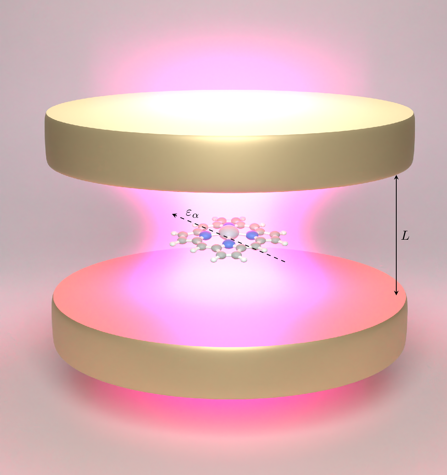
In the benchmark calculations presented below we consider the series of group 12 atoms (Zn, Cd, Hg), and a large mercury porphyrin (Hg@porphyrin). The geometry of the Hg porphyrin was taken from Ref. 135 and corresponds to a non-planar configuration of \ceC_4v symmetry.
All spectra were calculated using the relativistic spectroscopy DFT program ReSpect. [168] The reference orbitals for the linear response calculations were obtained from the ground state uncoupled to photons. The relativistic four-component molecular spinorbitals for electrons were described Gaussian-type orbital (GTO) basis sets where the scalar GTOs were used for the large component and the basis for the small-component basis was generated by imposing the restricted kinetically balanced (RKB) relation. [174] The selected scalar basis sets were the uncontracted Dyall’s VDZ basis sets for metals (Zn, Cd, Hg) [175, 176, 177, 178] and the uncontracted Dunning’s cc-pVDZ basis sets [179] for light elements. and the B3LYP XC approximation of the density functional. [180, 181, 182, 183, 184] The numerical integration of the noncollinear exchange–correlation potential and kernel was done with an adaptive molecular grid of medium size (program default). In the 4c calculations, atomic nuclei of finite size were approximated by a Gaussian charge distribution model.
The electron–photon correlation is treated under the photon random phase approximation (pRPA) [69, 72] which amounts to disregarding the photon–electron exchange–correlation potential and kernel in Eqs. (43) and (53c), respectively. Moreover, we consider the adiabatic approximation in the construction of the XC kernels, i.e. all dependencies on in Eqs. (53) are dropped. At present, we restrict ourselves to closed-shell systems for which the adiabatic noncollinear XC kernel has the form given in Eqs. 24-26c in Ref. 162. The eigenvalue equation was solved iteratively for the first 50 or 100 excitation energies for systems coupled to a single cavity mode. The spectra were subsequently evaluated from the excitation energies and transition moments obtained from the left and right eigenvectors, in the case of coupling to a single cavity mode, empirical Lorentzian broadening was used to obtain finite-width peaks.
IV Results and discussion
IV.1 Atoms with singlet–triplet transitions
First, we consider the case of atoms of group 12 metals, Zn, Cd, and Hg whose spectra were previously studied at the level of four-component Dirac–Coulomb Hamiltonian using linear response [185, 173] and real-time TDDFT [186]. The first two excited states correspond to the triplet state \ce^3P and the singlet state \ce^1P, where the transition from the \ce^1S0 ground state to the excited triplet state is forbidden in theories neglecting spin–orbit coupling (SOC). With SOC considered, the transition to \ce^3P1 becomes allowed while the transitions to the other two triplet components (\ce^3P0, \ce^3P2) remain forbidden due to the selection rule within the dipole approximation. The excitation energies for the allowed \ce^1S0 \ce^3P1 and \ce^1S0 \ce^1P1 transitions are summarized in Table S1 in the Supplemental Material while the calculated values reproduce reference experimental data [187] reasonably well given the functional and basis set size. Both the \ce^1S0 \ce^3P1 and \ce^1S0 \ce^1P1 transitions are composed of three degenerate spectral lines. In the orbital picture, the highest occupied shell corresponds to s orbitals and the lowest unoccupied to p while after SOC is taken into account the p shell splits into \cep_1/2 and \cep_3/2 levels. There are in total 12 possible single-electron excitations between s and \cep_1/2 and \cep_3/2 orbitals and these constitute the dominant contributions to TDDFT transition vectors. However, these 12 simple configurations cannot be straightforwardly identified with the components of the singlet and triplet excited states as their transition vectors contain more than one significant orbital pair contribution.
To investigate the effect of the strong coupling to photons on these atomic spectra, we solve the linear response QEDFT equation for a single atom coupled to a single effective cavity mode with the cavity frequency scanning the region around the singlet–triplet (S–T) and singlet–singlet (S–S) transitions. By focusing on a single efficient cavity mode, it is implied that the remaining spectrum of modes is accounted for by working with the renormalized (observable) masses of the electrons [7, 188].
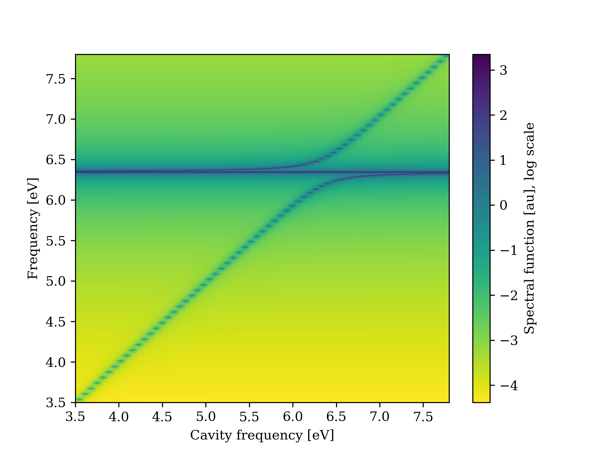
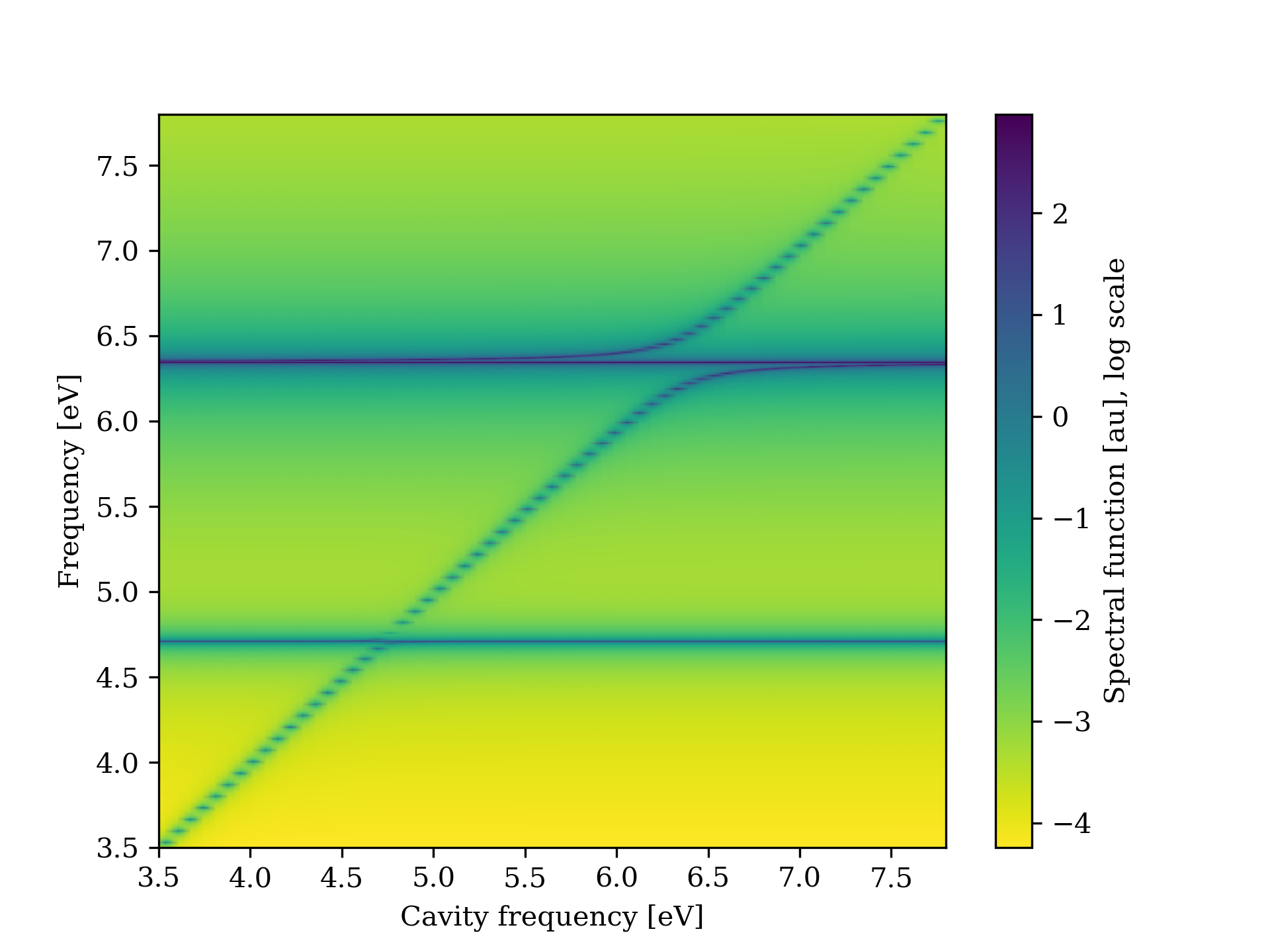
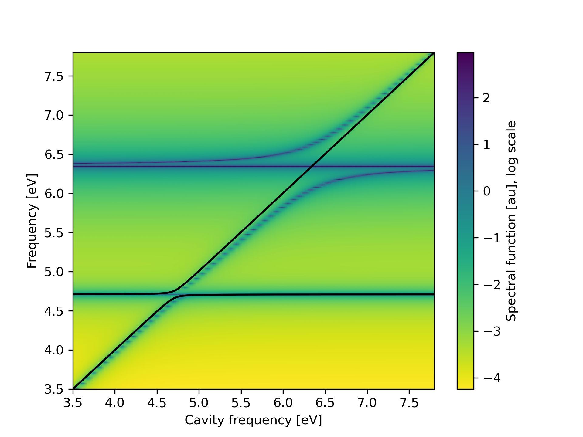
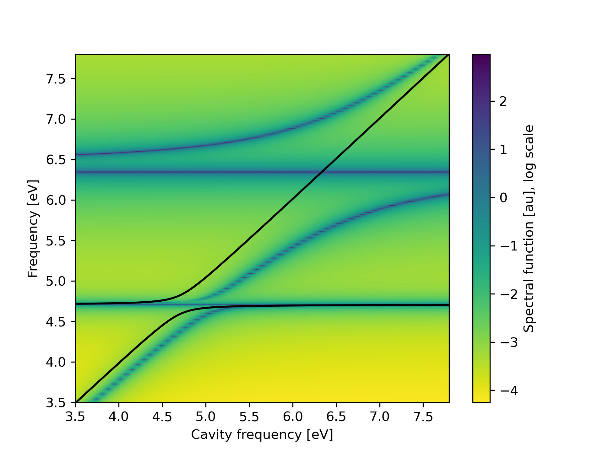
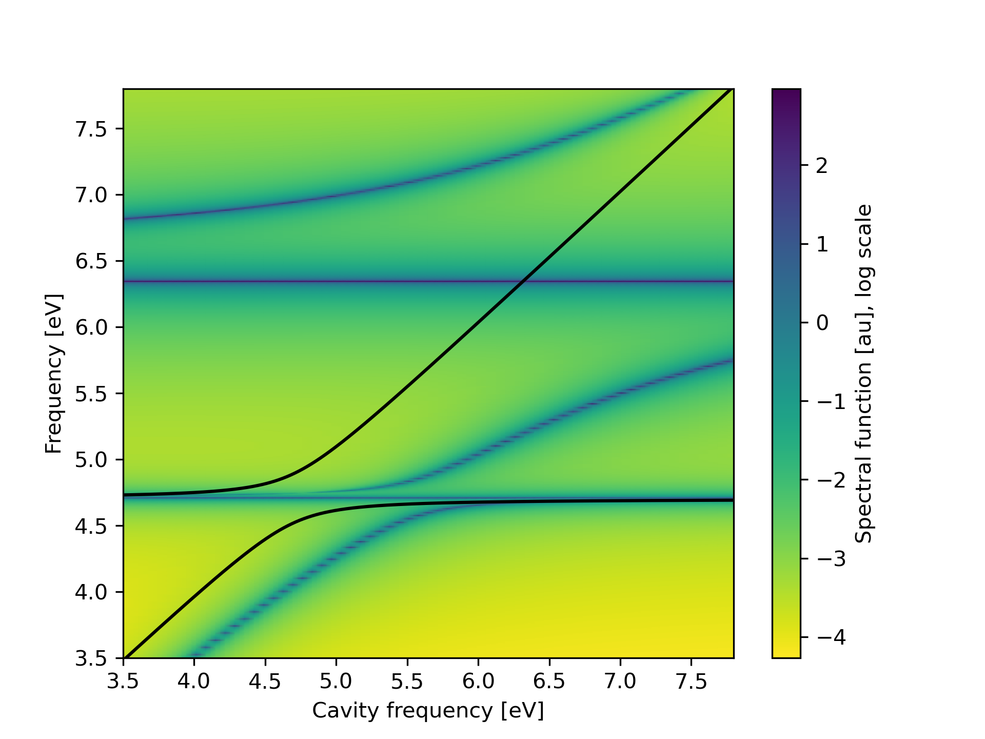
The results of series of calculations with different cavity frequencies are excitation energies and corresponding transition moments from which it is possible to calculate absorption spectra. Such spectra are depicted for Hg atom in Figure 2(c) showing both non-relativistic one-component (1c) and fully relativistic four-component (4c) calculations (results for Zn and Cd atoms are in the Supplemental Material, Figure S1). The -axis shows the cavity frequency, the -axis corresponds to excitation energy while the magnitude of the spectral function is depicted as the color gradient in logarithmic () scale to allow comparison between the S–T and S–S transitions of vastly different magnitudes. The spectra were artificially broadened using Lorentzian broadening with broadening parameter (see text after Eqs. (65)). Only excited states with nonzero transition dipole moments are visible as signals in the spectra, i.e. \ce^1P1 and \ce^3P1, while the other components of the triplet state with total angular momentum and are dark.
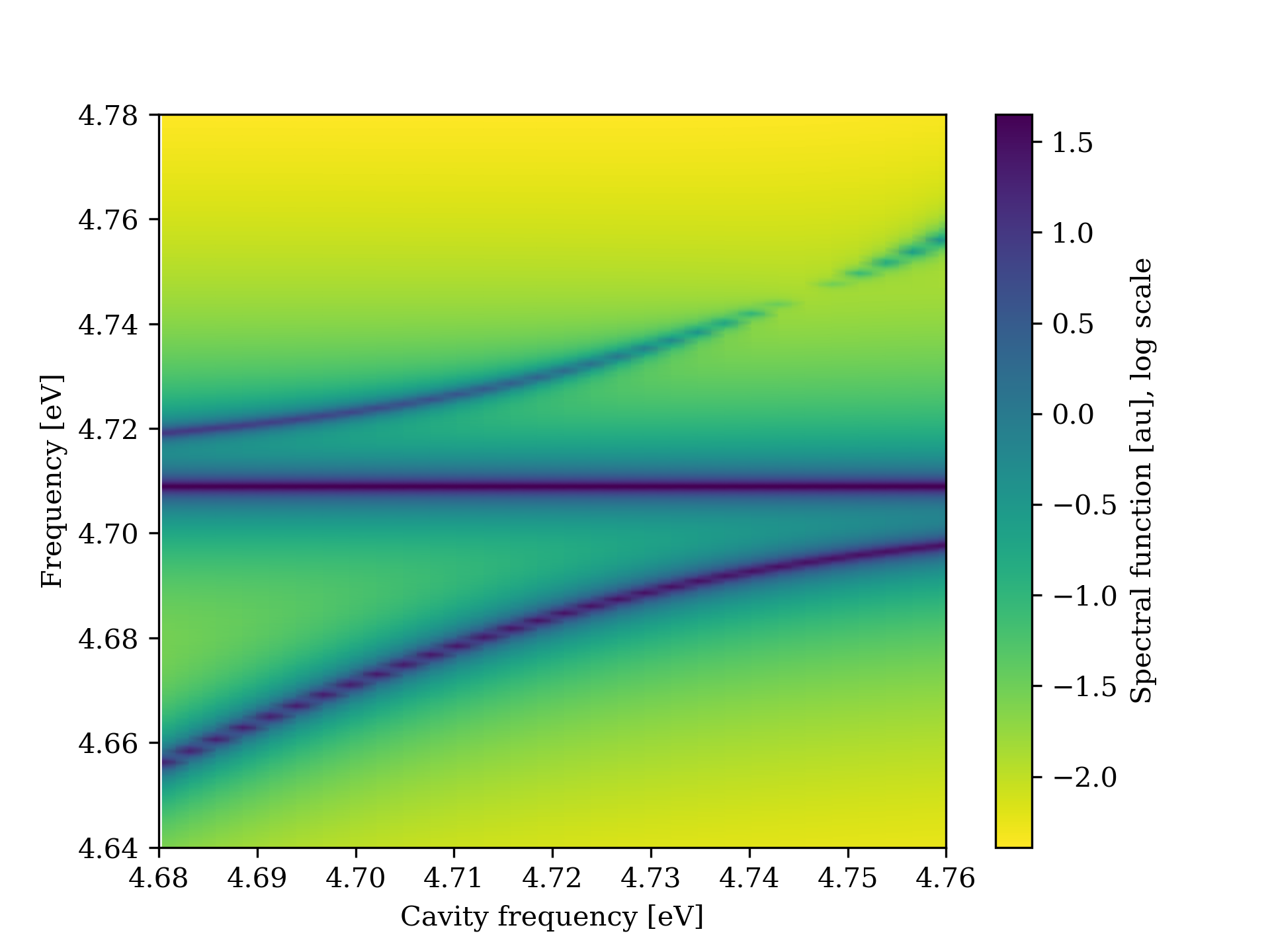
The plots depict a common scenario wherein light-matter mixing increases as the cavity frequency approaches a resonance with an excitation energy. Both the \ce^3P1 and \ce^1P1 excited states are originally triply degenerate with the degenerate levels having perpendicular transition dipole moments. Therefore, the photon state mixes with only one of the three states – the one with the transition dipole moment parallel with the photon polarization – and the uncoupled excitation energies are still visible due to the two remaining levels of both \ce^3P1 and \ce^1P1. When compared with the non-relativistic picture, the relativistic description causes a shift in the energy of the excited singlet state – the non-relativistic spectra were artificially shifted so that the S–S excitation energies would be aligned. The specific shifts were , , and , for Zn, Cd, and Hg, respectively. Furthermore, the inclusion of relativity introduces a transition to the excited triplet state. The intensity of the S–T transition as well as the spectral shifts are more prominent for heavier atoms. As the transition to the excited triplet state becomes allowed, a mixing with the cavity mode is observed near the resonant frequency. Since the coupling to the cavity mode is proportional to the transition dipole moment, which for the S–T transition increases with atomic number, the Rabi splitting of the polaritons originating from the triplet state is the largest for mercury. From the zoomed-in insets in the dispersion plots in Figure 2(c) we see that the maximum (50:50) light–matter mixing does not occur at exactly the S–T resonant frequency, but rather at a higher frequency. The maximum light-matter mixing around the S–S resonance also occurs at a frequency shifted from the resonance by approximately the same amount as the around the S–T transition.
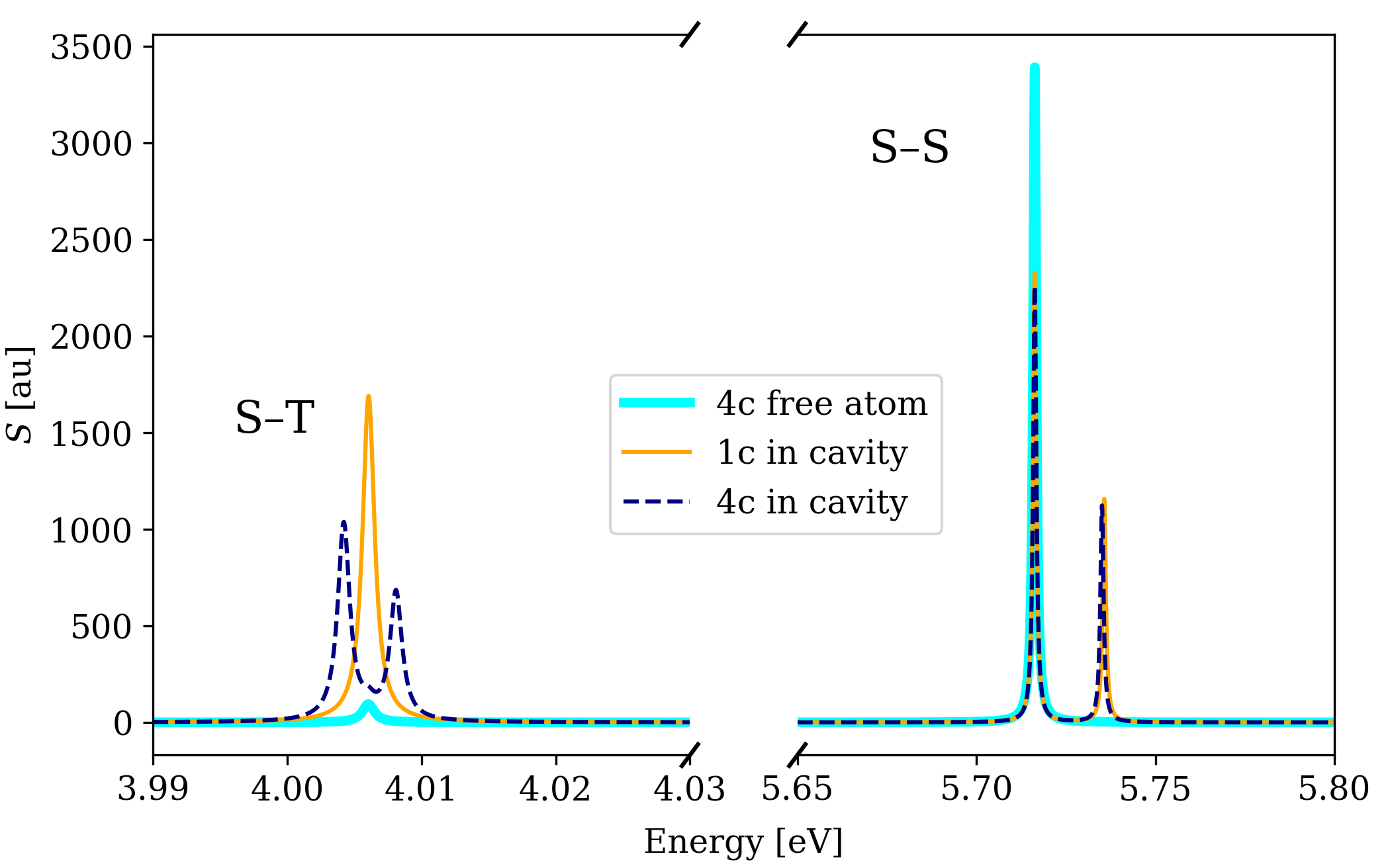
We calculated absorption spectra with cavities tuned to these maximum mixing frequencies, i.e. , , and , for Zn, Cd, and Hg, respectively. The spectra for Zn and Hg are depicted in Figure 3 while the spectrum for Cd is available in the Supplemental Material, Figure S2. As discussed above, two S–T transitions with perpendicular transition dipole are still present as excitation energies and visible in the spectra of Cd and Hg as a line with 2/3 of the intensity seen in the uncoupled system (for Zn, the extremely weak line corresponding to the uncoupled S–T transitions is obscured by peak broadening). In the spectral region around the S–T transition, the spectra contain very intense polaritonic peaks with the increase of the transition moment with respect to the original S–T transition ranging from a striking 50-fold increase for Zn to about 20% for Hg (compared to the intensity of one of the three degenerate states meaning that the peak composed of two degenerate uncoupled S–T states is more intense than the polaritonic peak in Hg).
While it is tempting to suggest an interpretation based on cavity enhancement of the S–T transition, it is important to note that the peak appears also in the one-component non-relativistic (1c) spectra. Since the 1c spectra are evaluated from the non-relativistic linear response calculations that do not contain the S–T transition, the peak must correspond to the lower polariton originating from the mixing of cavity mode with S–S exciton. Even if the cavity frequency is far from the resonance with the S–S transition and the polaritonic state is light-like (), its intensity is sufficient to be comparable with the S–T transition in the relativistic (4c) calculations. This is in agreement with the 2D spectra in Figure 2(c) where the intensity of the lower polaritonic branch in the 1c calculations is more intense (Zn) or comparable (Hg, also Cd) with the S–T transition in the 4c spectra.
In the 4c calculations, the effects of the coupling to the low-intensity S–T transition and the intense but off-resonant S–S transition combine. Besides the spectral signature in the S–T region discussed above, in the region around the S–S transition, one of the originally three degenerate spectral lines is blueshifted and its response vector contains a small but non-negligible () photonic contribution. Most of the intensity increase of the polaritonic peaks arising from the S–T transition is accounted for by the corresponding decrease in intensity of the shifted S–S transition. The decrease in intensity of the shifted S–S line is in fact larger than the gain of the S–T transition, with the gain being about 80% of the decrease. The Thomas–Reiche–Kuhn sum rule is then preserved by states higher in the spectrum when one state of three degenerate states is also slightly shifted in energy and its intensity is now higher. This repeats for all triply degenerate states at higher energies. The sum of photonic contributions from the lower and upper S–T polariton and the shifted S–S line is 1 with the accuracy of – and lower for the higher lying states. Note that in pRPA QEDFT with single cavity mode, the total sum of photon contributions should be 1 and only one extra peak can appear in the spectrum of an atom or molecule coupled to the cavity.
These results show the importance of the off-resonant coupling where the photon mode is coupled not only to the resonant S–T exciton but also to the off-resonant yet high-transition-moment S–S exciton as well as all higher-lying states. In turn, this demonstrates the importance of ab initio QEDFT treatment: a simple two-state model built from the S–T excitation energy and corresponding transition dipole moment would produce two polaritonic states whose intensity would sum to the original S–T intensity. Another effect beyond the two-state model is the shift of S–T resonance (50:50 light-matter mixing) toward higher frequencies. This becomes more pronounced as the coupling strength increases as shown in Figure 4(c). Here, the results of QEDFT calculations are compared with Jaynes–Cummings (JC) energies , where and with S–T excitation energy and transition dipole moment taken from a TDDFT calculation without coupling to cavity.
While models can be extended to account for more than two states, it is impossible to a priori say how many excited states should be included, particularly for systems with dense spectra such as molecules. Therefore, ab initio calculations are an indispensable tool for qualitative and quantitative predictions of properties of strongly bound light–matter systems, as well as for guiding the development of models. The quest to extend their capabilities to include further effects, such as relativity and spin–orbit coupling, is thus an important direction in polaritonic chemistry.
IV.2 Large molecular metal complex
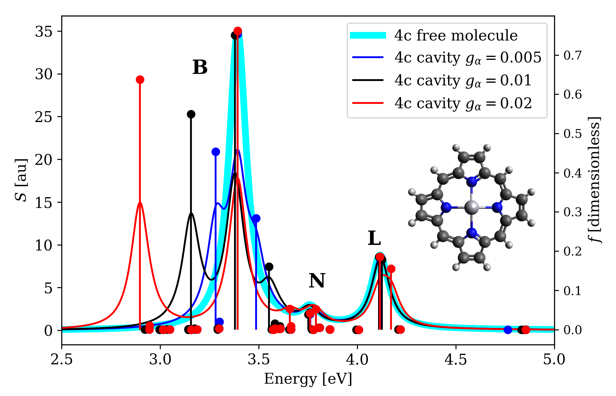
To demonstrate that our implementation is not restricted to atoms, but applicable also to large molecules containing heavy elements, we calculate the electron absorption spectrum of a mercury porphyrin inside a Fabry–Pérot cavity. Porphyrins are a class of molecules with important biological roles as well as technological applications and there is a large number of both experimental [189] and theoretical [190, 191] works devoted to their study including the modification of their properties in optical cavities. [139, 192, 193] Moreover, the absorption spectra of porphyrin complexes of group 12 atoms including the Hg porphyrin considered here, were studied before at the four-component relativistic level of theory by Fransson et al. [135] Note that unlike the reference work [135] we do not explicitly consider point group symmetry in our calculations thus performing an all-atom all-electron calculation in the ground state.
The spectrum of the free Hg-substituted porphyrin is dominated by the strong B-band at , while other notable features are the N- and L-bands at 3.76 and , respectively with the Q-band being very weak and not visible in this spectrum. All of these spectral lines arise from doubly degenerate excited states with perpendicular transition dipole moments, i.e. and for the molecule oriented such that its \ceC4 symmetry axis coincides with the axis. In the calculations of polaritonically modified spectra we consider the Hg porphyrin complex embedded in a Fabry–Pérot cavity with an effective single mode of frequency that is in resonance with the B band excitation energy with progressively stronger coupling constant . The resulting spectra together with the spectrum of the uncoupled system are depicted in Figure 5. While for the weakest coupling (dark blue line), the dominating modification of the spectrum due to the cavity is the splitting of one of the two degenerate B lines into an upper and lower polariton, for the stringer values of the coupling, other lines in the spectrum start to be affected as well. Particularly for we see breaking of the degeneracy in the form of frequency and intensity shifts of other spectral lines including the N and L lines. Therefore, besides demonstrating the readiness of our method for the treatment of chemically relevant molecules, these results also stress the importance of ab initio QED methods.
V Conclusions
In this article we presented the first implementation of a relativistic ab initio quantum electrodynamical method combining relativistic description of electronic structure with the treatment of transverse photons as dynamical variables in the form of linear response QEDFT based on the four-component Dirac–Kohn–Sham Hamiltonian. We presented a detailed theory derivation of the final electron–photon Hamiltonian starting from relativistic QED while keeping track of all approximations made on the way. For the linear response equations we showed how a spectral function can be calculated from a non-hermitian Casida-like equation by considering both the left and right eigenvectors, as well as showed how this equation can be transformed to the symmetric equation often considered in ab initio QEDFT literature.
We applied the developed method to the calculation of polaritonically modified spectra of heavy-element atoms with singlet–triplet transitions and demonstrated that the intensity of the transition can be enhanced by the coupling to the cavity as well showed the coupling between the singlet–singlet and singlet–triplet transitions via the cavity modes that results in non-resonant splitting of spectral lines as well the transfer of intensity between them. Of specific interest is that the cavity even in the long-wavelength limit can influence the SOC due to a fully relativistic (four-component) treatment of the electrons. Our results showing the interplay of off-resonant coupling and spin–orbit driven transition demonstrate the need for accurate ab initio methods such as QEDFT to describe cavity modification of molecular properties as well as help to guide the formulation of approximate models – in the cases presented a minimal two-state model would be insufficient in describing the cavity modified of spectra around the singlet–triplet resonance. Moreover, the linear response QEDFT methodology developed with the primary motivation of describing polaritonic chemistry in cavities allows to address other situations when electrons are coupled to photons as well. Such an example is the coupling to vacuum modes that presents a way of calculating radiative lifetimes from first principles thereby resolving one of the shortcomings of electronic-structure linear-response theories that add this variable as an empirical parameter. Finally by addressing the spectrum of mercury porphyrin in the cavity we demonstrated that our program is capable of handling even large molecules of chemical interest.
Ab initio QED methods have emerged recently as a first principles approach for the prediction and interpretation of phenomena occurring under strong coupling of electronic and vibrational degrees of freedom of a material to the photonic modes of an optical cavity. In this work, we expanded the toolbox of ab initio QED methods further by bringing them into the relativistic domain. Considering the advances in understanding also collective coupling effects [167, 159, 160] and the here presented changes in the SOC, we think that this toolbox can help to design cavity setups such that SOC and other relativistic effects can be enhanced. This also conceptually is very interesting since it highlights that the transverse photons, usually discarded when deriving relativistic quantum chemistry equations from full QED, can be decisive for real atomic and molecular systems. For instance, taking into account (approximately) the continuum of modes can be used to study non-perturbatively very fundamental effects of quantum field theories, such as the mass renormalization of the electrons [7]. We also showed how relativistic description of electronic structure of a material inside a photonic structure reveals the presence of a new type of spin–orbit interaction mediated by cavity photons. This opens a new avenue in the fields of cavity QED and polaritonic chemistry with a potential for follow-up works focused on singlet–triplet transitions in singlet fission systems, the exploration of the new SOC term in solid state systems, or the development of effective Hamiltonians.
Appendix A Notations and conventions
We use the following definitions: for contravariant four-vector, for covariant four-vector, is the metric tensor
and are the Dirac matrices in their standard representation
and the Pauli matrices
Here is a unit matrix
We use the italic style for scalars, boldface for three vectors, and Roman style for four-vectors and their components. Four vectors have the form and coordinates in four space are also denoted as . The scalar product of four-vectors is defined as . The summing over repeated indices is assumed by default. Fock space vectors and matrices are also denoted by Roman boldface with and denoting the unit and zero matrix, respectively.
Appendix B Solution of first order EOMs by undetermined coefficients
In the method of undetermined coefficients, we use the following ansatz for the electronic equation
| (68a) | ||||
| (68b) | ||||
motivated by the inhomogeneity in Eq. (52). Similarly, we formulate an ansatz for the photonic displacement coordinate in the form
| (69) |
from which follows
| (70) |
and where the real nature of was taken into account.
We consider only a single inhomogeneity in the whole system of equations at a time, i.e., the external field or the external current. The ansätze will then contain its respective frequency (i.e. or ). By inserting expressions from Eqs. (68)-(70) into Eqs. (60) and selecting only the terms with time dependence we obtain a set of coupled algebraic equations
| (71a) | ||||
| (71b) | ||||
| (71c) | ||||
Unfortunately, the equation for contains , a recurrence of the second order differential equation (57) as we would obtain the system of equations (71) also by considering Eq. (57) instead of Eqs. (58) and (59) for the photonic degrees of freedom. Since we want to get an equation linear in , we remove the second power by employing the identity
| (72) |
which transforms Eq. (71c) into
| (73) |
We can now divide into two components that satisfy Eq. (73) term by term
| (74a) | ||||
| (74b) | ||||
and both contain only in the first power. This way, we can write four coupled algebraic equations linear in for the variables , , , and that collected in a matrix give
| (75) |
where we defined
| (76) |
and is a diagonal matrix with elements on the diagonal. An analogous equation can be derived for the case of external current with the right-hand side having the form . This is the Sternheimer equation describing the response of a molecular system in a cavity to an external field of frequency coupled to the electronic subsystem via operator . The algebraic form of the homogeneous equation to the system (60) can now be obtained from Eq. (75) by discarding the right-hand side with the frequency of the external field gaining the meaning of a resonance frequency of the system, i.e. -th excitation energy , leading to Eq. (62).
Appendix C Solution of the matrix differential equation and the interpretation of photon terms
It is interesting to note that an alternative approach to Eq. (62) exists based on a direct solution of the coupled system of differential equations (60). This system corresponds to a matrix differential equation in the form , where
| (77a) | ||||
| (77b) | ||||
| (77c) | ||||
The homogeneous equation takes the form and its general solution is , where are the eigenvectors of matrix , their corresponding eigenvalues and constant coefficients. The solution of the homogeneous equation thus boils down to finding the eigenvectors and eigenvalues of the matrix defined in Eq. (77b). Since two matrices related by a similarity transformation have the same set of eigenvalues, one can alternatively solve the eigenproblem for its similar matrix with eigenvectors , if the new matrix has some more favorable properties. For example, matrix defined in Eq. (77b) can be transformed into a diagonally dominant matrix by
| (78) |
with the same definition of as above and matrices , , and corresponding to diagonal matrices with , , and , respectively, on the diagonal. This transformation recovers the matrix in Eq. (62) (after multiplication with the matrix on the right-hand side). Moreover, the similarity transformation also shows a relationship between the new photonic variables and , and the old and in the form
| (79a) | ||||
| (79b) | ||||
which is analogous but not yet identical to the definition of creation and annihilation operators in Eqs. (20) and (19), suggesting an interpretation of as a creation and as an annihilation amplitude, respectively.
Furthermore, we can perform yet another similarity transformation to symmetrize the matrix defined in Eq. (78),
| (80) |
where the photon–electron and the electron–photon coupling has the form
| (81) |
and matrices and are diagonal matrices with and , respectively, on the diagonal. Symmetrization in Eq. (80) recovered the matrix appearing in the Casida equation solved in some other works on linear response QEDFT. [70, 71] Furthermore, the symmetrizing similarity transform gives
| (82a) | ||||
| (82b) | ||||
which exactly corresponds to the definition of the creation and annihilation operators in Eqs. (20) and (19) giving and the meaning of creation and annihilation amplitudes, respectively.
Appendix D Derivation of the expression for polarizability using left and right eigenvectors
To compactify the following discussion, let us adopt the notation common in quantum chemistry where the Sternheimer equation (75) is written term-by-term as . and Eq. (63) takes the form . The right and left eigenvectors are defined as
| (83a) | ||||
| (83b) | ||||
where matrix is a diagonal matrix containing all the eigenvalues and the columns of matrices and contain all the right and left eigenvectors, respectively. Moreover, we made use of the fact that . Left and right eigenvectors corresponding to different eigenvalues are orthogonal, and can be transformed to be so for degenerate subspaces, meaning that their matrices satisfy . Let us note that the definition of as a left eigenvector of matrix is due to the computer implementation that solves the eigenproblem for matrix instead of the generalized eigenproblem. The alternative formulation of left eigenvectors stemming from the generalized eigenproblem is related to ours via and the eigenvectors satisfy the condition . From Eqs. (83) it also follows that .
The expression for the polarizability can be worked out as
| (84) | ||||
where we renamed to both for clarity as well as to indicate its meaning as the frequency at which the frequency-dependent polarizability is evaluated. The matrix is diagonal and can be easily inverted. However, the formula can be further simplified by taking into account the fact that the eigenvalues come in positive–negative pairs, i.e. the matrix has the structure
| (85) |
where is a diagonal matrix of the positive eigenvalues labeled from 1 to . Therefore, the expression for the polarizability tensor becomes
| (86) |
where variables labeled by and belong to excitation energies and , respectively, and the right and left transition dipole moments are defined as
| (87a) | |||||
| (87b) | |||||
The fact that only the electronic parts and of the transition vector are used to calculate the transition dipole moment in Eqs. (65) is the consequence of the fact that the electric dipole moment is an electron-only property described by . The eigenvector corresponding to an eigenvalue with the opposite sign has and , therefore and . After inserting these expressions into Eq. (86), we obtain the final expression for the frequency-dependent polarizability calculated from the distinct right and left eigenvectors
| (88) |
Supplemental Material
Additional spectra, JC model definition, geometry of the Hg@porphyrin.
ACKNOWLEDGMENTS
LK acknowledges support by the Research Council of Norway through its Centres of Excellence scheme, project no. 262695, and its Mobility Grant scheme, project no. 314814. LK would like to thank Stanislav Komorovsky, Johannes Flick, and Davis Welakuh for helpful discussions. VK would like to thank Simone Latini for the help in the preparation figure of the cavity. The calculations were performed on resources provided by Sigma2—the National Infrastructure for High Performance Computing and Data Storage in Norway, Grant Nos. NN4654K and NN14654K.
References
- [1] Thomas W. Ebbesen. Hybrid light–matter states in a molecular and material science perspective. Acc. Chem. Res., 49(11):2403–2412, 2016. PMID: 27779846.
- [2] Michael Ruggenthaler, Nicolas Tancogne-Dejean, Johannes Flick, Heiko Appel, and Angel Rubio. From a quantum-electrodynamical light–matter description to novel spectroscopies. Nat. Rev. Chem., 2(3):1–16, 2018.
- [3] Anton Frisk Kockum, Adam Miranowicz, Simone De Liberato, Salvatore Savasta, and Franco Nori. Ultrastrong coupling between light and matter. Nature Reviews Physics, 1(1):19–40, 2019.
- [4] Dmitri N Basov, Ana Asenjo-Garcia, P James Schuck, Xiaoyang Zhu, and Angel Rubio. Polariton panorama. Nanophotonics, 10(1):549–577, 2020.
- [5] Johannes Flick, Michael Ruggenthaler, Heiko Appel, and Angel Rubio. Kohn-Sham approach to quantum electrodynamical density- functional theory: Exact time-dependent effective potentials in real space. Proc. Natl. Acad. Sci. USA, 112:15285, 2015.
- [6] F. Schlawin, D. M. Kennes, and M. A. Sentef. Cavity quantum materials. Appl. Phys. Rev., 9(1):011312, 02 2022.
- [7] Michael Ruggenthaler, Dominik Sidler, and Angel Rubio. Understanding polaritonic chemistry from ab initio quantum electrodynamics. Chemical Reviews, 0(0):null, 0. PMID: 37729114.
- [8] C. Cohen-Tannoudji, J. Dupont-Roc, and G. Grynberg. Photons and Atoms-Introduction to Quantum Electrodynamics. Wiley-VCH, Weinheim, 1997.
- [9] Johannes Feist, Javier Galego, and Francisco J. Garcia-Vidal. Polaritonic chemistry with organic molecules. ACS Photonics, 5(1):205–216, 2018.
- [10] Tao E. Li, Abraham Nitzan, and Joseph E. Subotnik. On the origin of ground-state vacuum-field catalysis: Equilibrium consideration. J. Chem. Phys., 152(23):234107, 06 2020.
- [11] Dominik Sidler, Michael Ruggenthaler, Christian Schäfer, Enrico Ronca, and Angel Rubio. A perspective on ab initio modeling of polaritonic chemistry: The role of non-equilibrium effects and quantum collectivity. J. Chem. Phys., 156(23):230901, 06 2022.
- [12] Arkajit Mandal, Michael AD Taylor, Braden M Weight, Eric R Koessler, Xinyang Li, and Pengfei Huo. Theoretical advances in polariton chemistry and molecular cavity quantum electrodynamics. Chemical Reviews, 123(16):9786–9879, 2023.
- [13] Blake S Simpkins, Adam D Dunkelberger, and Igor Vurgaftman. Control, modulation, and analytical descriptions of vibrational strong coupling. Chem. Rev., 123(8):5020–5048, 2023.
- [14] D. Basov, R. Averitt, and D. Hseeh. Towards properties on demand in quantum materials. Nat. Mater., 16:1077–1088, 2017.
- [15] M. Buzzi, M. Först, R. Mankowsky, and A Cavalleri. Probing dynamics in quantum materials with femtosecond X-rays. Nat. Rev. Mater., 3:299–311, 2018.
- [16] Xiao Wang, Enrico Ronca, and Michael A. Sentef. Cavity quantum electrodynamical chern insulator: Towards light-induced quantized anomalous hall effect in graphene. Phys. Rev. B, 99:235156, Jun 2019.
- [17] Martin Kiffner, Jonathan R. Coulthard, Frank Schlawin, Arzhang Ardavan, and Dieter Jaksch. Manipulating quantum materials with quantum light. Phys. Rev. B, 99:085116, Feb 2019.
- [18] Jiajun Li, Denis Golez, Giacomo Mazza, Andrew J. Millis, Antoine Georges, and Martin Eckstein. Electromagnetic coupling in tight-binding models for strongly correlated light and matter. Phys. Rev. B, 101:205140, May 2020.
- [19] Yuto Ashida, Ataç İmamoğlu, and Eugene Demler. Cavity Quantum Electrodynamics at Arbitrary Light-Matter Coupling Strengths. Phys. Rev. Lett., 126:153603, Apr 2021.
- [20] James A Hutchison, Tal Schwartz, Cyriaque Genet, Eloïse Devaux, and Thomas W Ebbesen. Modifying chemical landscapes by coupling to vacuum fields. Angew. Chem. Int. Ed., 51(7):1592–1596, 2012.
- [21] Anoop Thomas, Jino George, Atef Shalabney, Marian Dryzhakov, Sreejith J. Varma, Joseph Moran, Thibault Chervy, Xiaolan Zhong, Eloïse Devaux, Cyriaque Genet, James A. Hutchison, and Thomas W. Ebbesen. Ground-state chemical reactivity under vibrational coupling to the vacuum electromagnetic field. Angew. Chem. Int. Ed., 55(38):11462–11466, 2016.
- [22] Xinyang Li, Arkajit Mandal, and Pengfei Huo. Cavity frequency-dependent theory for vibrational polariton chemistry. Nat. Commun., 12(1):1315, 2021.
- [23] Francisco J Garcia-Vidal, Cristiano Ciuti, and Thomas W Ebbesen. Manipulating matter by strong coupling to vacuum fields. Science, 373(6551):eabd0336, 2021.
- [24] Christian Schäfer, Johannes Flick, Enrico Ronca, Prineha Narang, and Angel Rubio. Shining light on the microscopic resonant mechanism responsible for cavity-mediated chemical reactivity. Nat. Commun., 13:7817, 2022.
- [25] Wonmi Ahn, Johan F Triana, Felipe Recabal, Felipe Herrera, and Blake S Simpkins. Modification of ground-state chemical reactivity via light–matter coherence in infrared cavities. Science, 380(6650):1165–1168, 2023.
- [26] Johannes Flick, Christian Schäfer, Michael Ruggenthaler, Heiko Appel, and Angel Rubio. Ab initio optimized effective potentials for real molecules in optical cavities: Photon contributions to the molecular ground state. ACS Photonics, 5(3):992–1005, 2018.
- [27] Simone Latini, Dongbin Shin, Shunsuke A. Sato, Christian Schäfer, Umberto De Giovannini, Hannes Hübener, and Angel Rubio. The ferroelectric photo ground state of \ceSrTiO3: Cavity materials engineering. Proc. Natl. Acad. Sci. U.S.A., 118(31):e2105618118, 2021.
- [28] Vasil Rokaj, Simeon I. Mistakidis, and H. R. Sadeghpour. Cavity induced collective behavior in the polaritonic ground state. SciPost Phys., 14:167, 2023.
- [29] Emil Vinas Boström, Adithya Sriram, Martin Claassen, and Angel Rubio. Controlling the magnetic state of the proximate quantum spin liquid -\ceRuCl3 with an optical cavity. arXiv:2211.07247, 2022.
- [30] David M. Coles, Yanshen Yang, Yaya Wang, Richard T. Grant, Robert A. Taylor, Semion K. Saikin, Alán Aspuru-Guzik, David G. Lidzey, Joseph Kuo-Hsiang Tang, and Jason M. Smith. Strong coupling between chlorosomes of photosynthetic bacteria and a confined optical cavity mode. Nat. Commun., 5:5561, 2014.
- [31] E. Orgiu, J. George, J. A. Hutchison, E. Devaux, J. F. Dayen, B. Doudin, F. Stellacci, C. Genet, J. Schachenmayer, C. Genes, G. Pupillo, P. Samori, and T. W. Ebbesen. Conductivity in organic semiconductors hybridized with the vacuum field. Nat. Mater, 14:1123–1129, 2015.
- [32] Johannes Schachenmayer, Claudiu Genes, Edoardo Tignone, and Guido Pupillo. Cavity-enhanced transport of excitons. Phys. Rev. Lett., 114(19):196403, 2015.
- [33] Xiaolan Zhong, Thibault Chervy, Shaojun Wang, Jino George, Anoop Thomas, James A. Hutchison, Eloise Devaux, Cyriaque Genet, and Thomas W. Ebbesen. Non-radiative energy transfer mediated by hybrid light-matter states. Angew. Chem. Int. Ed., 55(21):6202–6206, 2016.
- [34] Johannes Feist and Francisco J. Garcia-Vidal. Extraordinary exciton conductance induced by strong coupling. Phys. Rev. Lett., 114:196402, May 2015.
- [35] Kati Stranius, Manuel Hertzog, and Karl Börjesson. Selective manipulation of electronically excited states through strong light–matter interactions. Nat. Commun., 9(1):2273, 2018.
- [36] Ovidiu Cotleţ, Sina Zeytinoǧlu, Manfred Sigrist, Eugene Demler, and Ata ç Imamoǧlu. Superconductivity and other collective phenomena in a hybrid bose-fermi mixture formed by a polariton condensate and an electron system in two dimensions. Phys. Rev. B, 93:054510, Feb 2016.
- [37] M. A. Sentef, M. Ruggenthaler, and Rubio A. Cavity quantum-electrodynamical polaritonically enhanced electron- phonon coupling and its influence on superconductivity. Sci. Adv., 4:eaau6969, 2018.
- [38] Jonathan B. Curtis, Zachary M. Raines, Andrew A. Allocca, Mohammad Hafezi, and Victor M. Galitski. Cavity quantum eliashberg enhancement of superconductivity. Phys. Rev. Lett., 122:167002, Apr 2019.
- [39] Frank Schlawin, Andrea Cavalleri, and Dieter Jaksch. Cavity-mediated electron-photon superconductivity. Phys. Rev. Lett., 122:133602, Apr 2019.
- [40] Simone Latini, Enrico Ronca, Umberto De Giovannini, Hannes Hübener, and Angel Rubio. Cavity control of excitons in two-dimensional materials. Nano Lett., 19(6):3473–3479, 2019. PMID: 31046291.
- [41] Jesper Levinsen, Guangyao Li, and Meera M. Parish. Microscopic description of exciton-polaritons in microcavities. Phys. Rev. Res., 1:033120, Nov 2019.
- [42] Michael Förg, Léo Colombier, Robin K. Patel, Jessica Lindlau, Aditya D. Mohite, Hisato Yamaguchi, Mikhail M. Glazov, David Hunger, and Alexander Högele. Cavity-control of interlayer excitons in van der waals heterostructures. Nat. Commun., 10(1):3697, Aug 2019.
- [43] J. Kasprzak, M. Richard, S. Kundermann, A. Baas, P. Jeambrun, J. M. J. Keeling, F. M. Marchetti, M. H. Szymańska, R. André, J. L. Staehli, V. Savona, P. B. Littlewood, B. Deveaud, and Le Si Dang. Bose–einstein condensation of exciton polaritons. Nature, 443(7110):409–414, Sep 2006.
- [44] Jonathan Keeling and Stéphane Kéna-Cohen. Bose–Einstein Condensation of Exciton-Polaritons in Organic Microcavities. Annu. Rev. Phys. Chem., 71(1):435–459, 2020. PMID: 32126177.
- [45] David Hagenmüller, Simone De Liberato, and Cristiano Ciuti. Ultrastrong coupling between a cavity resonator and the cyclotron transition of a two-dimensional electron gas in the case of an integer filling factor. Phys. Rev. B, 81:235303, Jun 2010.
- [46] G. Scalari, C. Maissen, D. Turčinková, D. Hagenmüller, S. De Liberato, C. Ciuti, C. Reichl, D. Schuh, W. Wegscheider, M. Beck, and J. Faist. Ultrastrong coupling of the cyclotron transition of a 2d electron gas to a thz metamaterial. Science, 335(6074):1323–1326, 2012.
- [47] Xinwei Li, Motoaki Bamba, Qi Zhang, Saeed Fallahi, Geoff C. Gardner, Weilu Gao, Minhan Lou, Katsumasa Yoshioka, Michael J. Manfra, and Junichiro Kono. Vacuum bloch–siegert shift in landau polaritons with ultra-high cooperativity. Nat. Photon., 12(6):324–329, Jun 2018.
- [48] Janine Keller, Giacomo Scalari, Felice Appugliese, Shima Rajabali, Mattias Beck, Johannes Haase, Christian A. Lehner, Werner Wegscheider, Michele Failla, Maksym Myronov, David R. Leadley, James Lloyd-Hughes, Pierre Nataf, and Jérôme Faist. Landau polaritons in highly nonparabolic two-dimensional gases in the ultrastrong coupling regime. Phys. Rev. B, 101:075301, Feb 2020.
- [49] Vasil Rokaj, Markus Penz, Michael A Sentef, Michael Ruggenthaler, and Angel Rubio. Polaritonic Hofstadter butterfly and cavity control of the quantized Hall conductance. Phys. Rev. B, 105(20):205424, 2022.
- [50] Sylvain Ravets, Patrick Knüppel, Stefan Faelt, Ovidiu Cotlet, Martin Kroner, Werner Wegscheider, and Atac Imamoglu. Polaron polaritons in the integer and fractional quantum hall regimes. Phys. Rev. Lett., 120:057401, Jan 2018.
- [51] Stephan Smolka, Wolf Wuester, Florian Haupt, Stefan Faelt, Werner Wegscheider, and Ataç Imamoglu. Cavity quantum electrodynamics with many-body states of a two-dimensional electron gas. Science, 346(6207):332–335, 2014.
- [52] Gian L. Paravicini-Bagliani, Felice Appugliese, Eli Richter, Federico Valmorra, Janine Keller, Mattias Beck, Nicola Bartolo, Clemens Rössler, Thomas Ihn, Klaus Ensslin, Cristiano Ciuti, Giacomo Scalari, and Jérôme Faist. Magneto-transport controlled by landau polariton states. Nat. Phys., 15(2):186–190, Feb 2019.
- [53] Jan Petersen, Jürgen Volz, and Arno Rauschenbeutel. Chiral nanophotonic waveguide interface based on spin-orbit interaction of light. Science, 346(6205):67–71, 2014.
- [54] Peter Lodahl, Sahand Mahmoodian, Søren Stobbe, Arno Rauschenbeutel, Philipp Schneeweiss, Jürgen Volz, Hannes Pichler, and Peter Zoller. Chiral quantum optics. Nature, 541(7638):473–480, Jan 2017.
- [55] Fan Zhang, Juanjuan Ren, Lingxiao Shan, Xueke Duan, Yan Li, Tiancai Zhang, Qihuang Gong, and Ying Gu. Chiral cavity quantum electrodynamics with coupled nanophotonic structures. Phys. Rev. A, 100:053841, Nov 2019.
- [56] Hannes Hübener, Umberto De Giovannini, Christian Schäfer, Johan Andberger, Michael Ruggenthaler, Jerome Faist, and Angel Rubio. Engineering quantum materials with chiral optical cavities. Nat. Mater., 20(4):438–442, Apr 2021.
- [57] Rohit Chikkaraddy, Bart De Nijs, Felix Benz, Steven J Barrow, Oren A Scherman, Edina Rosta, Angela Demetriadou, Peter Fox, Ortwin Hess, and Jeremy J Baumberg. Single-molecule strong coupling at room temperature in plasmonic nanocavities. Nature, 535(7610):127–130, 2016.
- [58] Alexey V Kavokin, Jeremy J Baumberg, Guillaume Malpuech, and Fabrice P Laussy. Microcavities, volume 21. Oxford university press, 2017.
- [59] Edwin T Jaynes and Frederick W Cummings. Comparison of quantum and semiclassical radiation theories with application to the beam maser. Proc. IEEE, 51(1):89–109, 1963.
- [60] Robert H Dicke. Coherence in spontaneous radiation processes. Phys. Rev., 93(1):99, 1954.
- [61] Jonathan J Foley IV, Jonathan F McTague, and A Eugene DePrince III. Ab initio methods for polariton chemistry. arXiv:2307.04881, 2023.
- [62] Michael Ruggenthaler, F Mackenroth, and Dieter Bauer. Time-dependent kohn-sham approach to quantum electrodynamics. Phys. Rev. A, 84(4):042107, 2011.
- [63] Michael Ruggenthaler, Johannes Flick, Camilla Pellegrini, Heiko Appel, Ilya V. Tokatly, and Angel Rubio. Quantum-electrodynamical density-functional theory: Bridging quantum optics and electronic-structure theory. Phys. Rev. A, 90:012508, 2014.
- [64] I. V. Tokatly. Time-dependent density functional theory for many-electron systems interacting with cavity photons. Phys. Rev. Lett., 110:233001, 2013.
- [65] Michael Ruggenthaler. Ground-state quantum-electrodynamical density-functional theory. arXiv:1509.01417, 2015.
- [66] Markus Penz, Erik I. Tellgren, Mihály A. Csirik, Michael Ruggenthaler, and Andre Laestadius. The Structure of the Density-Potential Mapping. Part II: Including Magnetic Fields. ACS Phys. Chem Au, 0(0):null, 0.
- [67] Soeren Ersbak Bang Nielsen, Christian Schäfer, Michael Ruggenthaler, and Angel Rubio. Dressed-orbital approach to cavity quantum electrodynamics and beyond. arXiv preprint arXiv:1812.00388, 2018.
- [68] Johannes Flick, Michael Ruggenthaler, Heiko Appel, and Angel Rubio. Atoms and molecules in cavities, from weak to strong coupling in quantum-electrodynamics (QED) chemistry. Proc. Natl. Acad. Sci. USA, 114:3026, 2017.
- [69] Johannes Flick, Davis M Welakuh, Michael Ruggenthaler, Heiko Appel, and Angel Rubio. Light–matter response in nonrelativistic quantum electrodynamics. ACS Photonics, 6(11):2757–2778, 2019.
- [70] Junjie Yang, Qi Ou, Zheng Pei, Hua Wang, Binbin Weng, Zhigang Shuai, Kieran Mullen, and Yihan Shao. Quantum-electrodynamical time-dependent density functional theory within Gaussian atomic basis. J. Chem. Phys., 155(6):064107, 2021.
- [71] Marcus D Liebenthal, Nam Vu, and A Eugene DePrince III. Mean-field cavity effects in quantum electrodynamics density functional and coupled-cluster theories. arXiv:2303.10821, 2023.
- [72] Davis M Welakuh, Johannes Flick, Michael Ruggenthaler, Heiko Appel, and Angel Rubio. Frequency-Dependent Sternheimer Linear-Response Formalism for Strongly Coupled Light–Matter Systems. J. Chem. Theory Comput., 18(7):4354–4365, 2022.
- [73] So Hirata and Martin Head-Gordon. Time-dependent density functional theory within the Tamm–Dancoff approximation. Chem. Phys. Lett., 314(3-4):291–299, 1999.
- [74] Florian Buchholz, Iris Theophilou, Soeren EB Nielsen, Michael Ruggenthaler, and Angel Rubio. Reduced density-matrix approach to strong matter-photon interaction. ACS Photonics, 6(11):2694–2711, 2019.
- [75] Tor S Haugland, Enrico Ronca, Eirik F Kjønstad, Angel Rubio, and Henrik Koch. Coupled cluster theory for molecular polaritons: Changing ground and excited states. Phys. Rev. X, 10(4):041043, 2020.
- [76] Florian Buchholz, Iris Theophilou, Klaas J. H. Giesbertz, Michael Ruggenthaler, and Angel Rubio. Light–matter hybrid-orbital-based first-principles methods: The influence of polariton statistics. J. Chem. Theory Comput., 16(9):5601–5620, 2020. PMID: 32692551.
- [77] Uliana Mordovina, Callum Bungey, Heiko Appel, Peter J. Knowles, Angel Rubio, and Frederick R. Manby. Polaritonic coupled-cluster theory. Phys. Rev. Res., 2:023262, Jun 2020.
- [78] Jonathan McTague and Jonathan J Foley. Non-Hermitian cavity quantum electrodynamics–configuration interaction singles approach for polaritonic structure with ab initio molecular Hamiltonians. J. Chem. Phys., 156(15), 2022.
- [79] Pedro Miguel M. C. de Melo and Andrea Marini. Unified theory of quantized electrons, phonons, and photons out of equilibrium: A simplified ab initio approach based on the generalized baym-kadanoff ansatz. Phys. Rev. B, 93:155102, Apr 2016.
- [80] Pekka Pyykkö. Relativistic effects in chemistry: more common than you thought. Annu. Rev. Phys. Chem., 63:45–64, 2012.
- [81] Pekka Pyykko and Jean Paul Desclaux. Relativity and the periodic system of elements. Acc. Chem. Res., 12(8):276–281, 1979.
- [82] P Romaniello and PL de Boeij. Relativistic two-component formulation of time-dependent current-density functional theory: Application to the linear response of solids. J. Chem. Phys., 127(17):174111, 2007.
- [83] Florent Calvo, Elke Pahl, Michael Wormit, and Peter Schwerdtfeger. Evidence for low-temperature melting of mercury owing to relativity. Angew. Chem. Int. Ed., 52(29):7583–7585, 2013.
- [84] Rajeev Ahuja, Andreas Blomqvist, Peter Larsson, Pekka Pyykkö, and Patryk Zaleski-Ejgierd. Relativity and the lead-acid battery. Phys. Rev. Lett., 106(1):018301, 2011.
- [85] V. P. Kosheleva, A. V. Volotka, D. A. Glazov, D. V. Zinenko, and S. Fritzsche. factor of lithiumlike silicon and calcium: Resolving the disagreement between theory and experiment. Phys. Rev. Lett., 128:103001, Mar 2022.
- [86] D. A. Glazov, F. Köhler-Langes, A. V. Volotka, K. Blaum, F. Heiße, G. Plunien, W. Quint, S. Rau, V. M. Shabaev, S. Sturm, and G. Werth. factor of lithiumlike silicon: New challenge to bound-state qed. Phys. Rev. Lett., 123:173001, Oct 2019.
- [87] Robert Laskowski and Peter Blaha. Understanding the l 2, 3 x-ray absorption spectra of early 3 d transition elements. Phys. Rev. B, 82(20):205104, 2010.
- [88] Nanna Holmgaard List, Trond Saue, and Patrick Norman. Rotationally averaged linear absorption spectra beyond the electric-dipole approximation. Mol. Phys., 115(1-2):63–74, June 2016.
- [89] Marta L Vidal, Pavel Pokhilko, Anna I Krylov, and Sonia Coriani. Equation-of-motion coupled-cluster theory to model L-edge x-ray absorption and photoelectron spectra. J. Phys. Chem. Lett., 11(19):8314–8321, 2020.
- [90] Joseph M. Kasper, Torin F. Stetina, Andrew J. Jenkins, and Xiaosong Li. Ab initio methods for L-edge x-ray absorption spectroscopy. Chem. Phys. Rev., 1(1):011304, December 2020.
- [91] Lukas Konecny, Jan Vicha, Stanislav Komorovsky, Kenneth Ruud, and Michal Repisky. Accurate X-ray Absorption Spectra near L- and M-Edges from Relativistic Four-Component Damped Response Time-Dependent Density Functional Theory. Inorg. Chem., 61(2):830–846, 2022.
- [92] Peter Hrobarik, Veronika Hrobarikova, Florian Meier, Michal Repisky, Stanislav Komorovsky, and Martin Kaupp. Relativistic four-component dft calculations of 1h nmr chemical shifts in transition-metal hydride complexes: unusual high-field shifts beyond the buckingham–stephens model. J. Phys. Chem. A, 115(22):5654–5659, 2011.
- [93] Peter Hrobarik, Veronika Hrobarikova, Anja H Greif, and Martin Kaupp. Giant spin-orbit effects on nmr shifts in diamagnetic actinide complexes: Guiding the search of uranium (vi) hydride complexes in the correct spectral range. Angew. Chem. Int. Ed., 51(43):10884–10888, 2012.
- [94] Jan Vicha, Radek Marek, and Michal Straka. High-frequency\ce^13C and \ce^29Si NMR chemical shifts in diamagnetic low-valence compounds of \ceTl^I and \cePb^II: Decisive role of relativistic effects. Inorg. Chem., 55(4):1770–1781, January 2016.
- [95] Jan Vicha, Jan Novotny, Stanislav Komorovsky, Michal Straka, Martin Kaupp, and Radek Marek. Relativistic heavy-neighbor-atom effects on nmr shifts: Concepts and trends across the periodic table. Chem. Rev., 120(15):7065–7103, 2020.
- [96] Bob Martin and Jochen Autschbach. Temperature dependence of contact and dipolar NMR chemical shifts in paramagnetic molecules. J. Chem. Phys., 142(5), February 2015.
- [97] Jan Novotny, Martin Sojka, Stanislav Komorovsky, Marek Necas, and Radek Marek. Interpreting the paramagnetic NMR spectra of potential ru(III) metallodrugs: Synergy between experiment and relativistic DFT calculations. J. Am. Chem. Soc., 138(27):8432–8445, July 2016.
- [98] Arobendo Mondal, Michael W. Gaultois, Andrew J. Pell, Marcella Iannuzzi, Clare P. Grey, Jürg Hutter, and Martin Kaupp. Large-scale computation of nuclear magnetic resonance shifts for paramagnetic solids using CP2k. J. Chem. Theory Comp., 14(1):377–394, December 2017.
- [99] Peter John Cherry, Syed Awais Rouf, and Juha Vaara. Paramagnetic enhancement of nuclear spin–spin coupling. J. Chem. Theory Comput., 13(3):1275–1283, February 2017.
- [100] Stanislav Komorovsky. Relativistic theory of EPR and (p)NMR. In Reference Module in Chemistry, Molecular Sciences and Chemical Engineering. Elsevier, 2023.
- [101] Irina Malkin, Olga L. Malkina, Vladimir G. Malkin, and Martin Kaupp. Relativistic two-component calculations of electronic g-tensors that include spin polarization. J. Chem. Phys., 123(24), December 2005.
- [102] Peter Hrobarik, Michal Repisky, Stanislav Komorovsky, Veronika Hrobarikova, and Martin Kaupp. Assessment of higher-order spin–orbit effects on electronic g-tensors of transition-metal complexes by relativistic two-and four-component methods. Theor. Chem. Acc., 129:715–725, 2011.
- [103] Sebastian Gohr, Peter Hrobarik, Michal Repisky, Stanislav Komorovsky, Kenneth Ruud, and Martin Kaupp. Four-component relativistic density functional theory calculations of epr g-and hyperfine-coupling tensors using hybrid functionals: validation on transition-metal complexes with large tensor anisotropies and higher-order spin–orbit effects. J. Phys. Chem. A, 119(51):12892–12905, 2015.
- [104] Hélène Bolvin and Jochen Autschbach. Relativistic methods for calculating electron paramagnetic resonance (EPR) parameters. In Handbook of Relativistic Quantum Chemistry, pages 725–763. Springer Berlin Heidelberg, October 2016.
- [105] Debora Misenkova, Florian Lemken, Michal Repisky, Jozef Noga, Olga L. Malkina, and Stanislav Komorovsky. The four-component DFT method for the calculation of the EPR g-tensor using a restricted magnetically balanced basis and london atomic orbitals. J. Chem. Phys., 157(16), October 2022.
- [106] Ben Joseph R. Cuyacot, Jan Novotny, Raphael J. F. Berger, Stanislav Komorovsky, and Radek Marek. Relativistic spin–orbit electronegativity and the chemical bond between a heavy atom and a light atom. Chem. Eur. J., 28(24), April 2022.
- [107] Taye B. Demissie, Brady D. Garabato, Kenneth Ruud, and Pawel M. Kozlowski. Mercury methylation by cobalt corrinoids: Relativistic effects dictate the reaction mechanism. Angew. Chem. Int. Ed., 55:11503–11506, 2016.
- [108] Torsha Moitra, Pijush Karak, Sayantani Chakraborty, Kenneth Ruud, and Swapan Chakrabarti. Behind the scenes of spin-forbidden decay pathways in transition metal complexes. Phys. Chem. Chem. Phys., 23(1):59–81, 2021.
- [109] V Pershina. Electronic structure and properties of superheavy elements. Nucl. Phys. A, 944:578–613, 2015.
- [110] S.A. Giuliani, Z. Matheson, W. Nazarewicz, E. Olsen, P.-G. Reinhard, J. Sadhukhan, B. Schuetrumpf, N. Schunck, and P. Schwerdtfeger. Colloquium: Superheavy elements: Oganesson and beyond. Rev. Mod. Phys., 91(1), January 2019.
- [111] Marius Kadek, Baokai Wang, Marc Joosten, Wei-Chi Chiu, Francois Mairesse, Michal Repisky, Kenneth Ruud, and Arun Bansil. Band structures and \ceZ2 invariants of two-dimensional transition metal dichalcogenide monolayers from fully relativistic dirac-kohn-sham theory using gaussian-type orbitals. Phys. Rev. Mater., 7(6):064001, 2023.
- [112] EI Rashba and E Ya Sherman. Spin-orbital band splitting in symmetric quantum wells. Phys. Lett. A, 129(3):175–179, 1988.
- [113] Martin Gmitra, Sergej Konschuh, Christian Ertler, Claudia Ambrosch-Draxl, and Jaroslav Fabian. Band-structure topologies of graphene: Spin-orbit coupling effects from first principles. Phys. Rev. B, 80(23):235431, 2009.
- [114] Zhiyong Y Zhu, Yingchun C Cheng, and Udo Schwingenschlögl. Giant spin-orbit-induced spin splitting in two-dimensional transition-metal dichalcogenide semiconductors. Phys. Rev. B, 84(15):153402, 2011.
- [115] Andreas Hermann, Jürgen Furthmüller, Heinz W Gäggeler, and Peter Schwerdtfeger. Spin-orbit effects in structural and electronic properties for the solid state of the group-14 elements from carbon to superheavy element 114. Phys. Rev. B, 82(15):155116, 2010.
- [116] K. G. Dyall and K. Faegri Jr. Introduction to Relativistic Quantum Chemistry. Oxford University Press, New York, 2007.
- [117] Markus Reiher and Alexander Wolf. Relativistic Quantum Chemistry: The Fundamental Theory of Molecular Science; 2nd Edition. Wiley-VCH, 2014.
- [118] Trond Saue. Relativistic Hamiltonians for chemistry: A primer. ChemPhysChem, 12(17):3077–3094, 2011.
- [119] Matthew S. Kelley and Toru Shiozaki. Large-scale Dirac–Fock–Breit method using density fitting and 2-spinor basis functions. J. Chem. Phys., 138(20), May 2013.
- [120] Shichao Sun, Jordan Ehrman, Tianyuan Zhang, Qiming Sun, Kenneth G Dyall, and Xiaosong Li. Scalar breit interaction for molecular calculations. J. Chem. Phys., 158(17), 2023.
- [121] Chad E Hoyer, Lixin Lu, Hang Hu, Kirill D Shumilov, Shichao Sun, Stefan Knecht, and Xiaosong Li. Correlated dirac–coulomb–breit multiconfigurational self-consistent-field methods. J. Chem. Phys., 158(4), 2023.
- [122] BJ Mackenzie, IP Grant, and PH Norrington. Program to calculate transverse breit and qed corrections to energy levels in a multiconfiguration dirac-fock environment. Comput. Phys. Commun.;(Netherlands), 21(2), 1980.
- [123] VM Shabaev, II Tupitsyn, and VA Yerokhin. Model operator approach to the lamb shift calculations in relativistic many-electron atoms. Phys. Rev. A, 88(1):012513, 2013.
- [124] Gustavo A Aucar. Toward a QFT-based theory of atomic and molecular properties. Phys. Chem. Chem. Phys., 16(10):4420–4438, 2014.
- [125] Peter Schwerdtfeger, Lukas F Pašteka, Andrew Punnett, and Patrick O Bowman. Relativistic and quantum electrodynamic effects in superheavy elements. Nucl. Phys. A, 944:551–577, 2015.
- [126] LF Pašteka, E Eliav, A Borschevsky, U Kaldor, and P Schwerdtfeger. Relativistic coupled cluster calculations with variational quantum electrodynamics resolve the discrepancy between experiment and theory concerning the electron affinity and ionization potential of gold. Phys. Rev. Lett., 118(2):023002, 2017.
- [127] AV Malyshev, DA Glazov, VM Shabaev, II Tupitsyn, VA Yerokhin, and VA Zaytsev. Model-qed operator for superheavy elements. Phys. Rev. A, 106(1):012806, 2022.
- [128] Ayaki Sunaga, Maen Salman, and Trond Saue. 4-component relativistic Hamiltonian with effective QED potentials for molecular calculations. arXiv:2207.14101v1.
- [129] Nobuki Inoue, Yoshihiro Watanabe, and Haruyuki Nakano. Theoretical examination of QED Hamiltonian in relativistic molecular orbital theory. J. Chem. Phys., 159(5), 2023.
- [130] Werner Kutzelnigg and Wenjian Liu. Quasirelativistic theory equivalent to fully relativistic theory. J. Chem. Phys., 123(24):241102, December 2005.
- [131] Wenjian Liu and Werner Kutzelnigg. Quasirelativistic theory. II. theory at matrix level. J. Chem. Phys., 126(11):114107, March 2007.
- [132] Miroslav Ilias and Trond Saue. An infinite-order two-component relativistic hamiltonian by a simple one-step transformation. J. Chem. Phys., 126(6):064102, February 2007.
- [133] Stefan Knecht, Michal Repisky, Hans Jørgen Aagaard Jensen, and Trond Saue. Exact two-component hamiltonians for relativistic quantum chemistry: Two-electron picture-change corrections made simple. J. Chem. Phys., 157(11):114106, 2022.
- [134] Can Liao, Joseph M Kasper, Andrew J Jenkins, Ping Yang, Enrique R Batista, Michael J Frisch, and Xiaosong Li. State interaction linear response time-dependent density functional theory with perturbative spin–orbit coupling: Benchmark and perspectives. JACS Au, 3(2):358–367, 2023.
- [135] Thomas Fransson, Trond Saue, and Patrick Norman. Four-component damped density functional response theory study of UV/Vis absorption spectra and phosphorescence parameters of group 12 metal-substituted porphyrins. J. Chem. Theory Comput., 12(5):2324–2334, 2016.
- [136] Hans Ågren, Olav Vahtras, and Boris Minaev. Response theory and calculations of spin-orbit coupling phenomena in molecules. In Advances in Quantum Chemistry, volume 27, pages 71–162. Elsevier, 1996.
- [137] Clàudia Climent, David Casanova, Johannes Feist, and Francisco J Garcia-Vidal. Not dark yet for strong light-matter coupling to accelerate singlet fission dynamics. Cell Rep., 3(4), 2022.
- [138] Elad Eizner, Luis A Martínez-Martínez, Joel Yuen-Zhou, and Stéphane Kéna-Cohen. Inverting singlet and triplet excited states using strong light-matter coupling. Sci. Adv., 5(12):eaax4482, 2019.
- [139] S Kéna-Cohen and SR Forrest. Green polariton photoluminescence using the red-emitting phosphor PtOEP. Phys. Rev. B, 76(7):075202, 2007.
- [140] Manuel Hertzog, Mao Wang, Jürgen Mony, and Karl Börjesson. Strong light–matter interactions: a new direction within chemistry. Chem. Soc. Rev., 48(3):937–961, 2019.
- [141] Xiaodong Xu, Wang Yao, Di Xiao, and Tony F Heinz. Spin and pseudospins in layered transition metal dichalcogenides. Nat. Phys., 10(5):343–350, 2014.
- [142] See-Hun Yang, Ron Naaman, Yossi Paltiel, and Stuart SP Parkin. Chiral spintronics. Nat. Rev. Phys., 3(5):328–343, 2021.
- [143] Herbert Spohn. Dynamics of charged particles and their radiation field. Cambridge university press, 2004.
- [144] Fumio Hiroshima. Ground states of quantum field models: perturbation of embedded eigenvalues, volume 35. Springer, 2019.
- [145] Lewis H Ryder. Quantum field theory. Cambridge university press, 1996.
- [146] Franz Mandl and Graham Shaw. Quantum field theory. John Wiley & Sons, 2010.
- [147] Toshimitsu Takaesu. On the spectral analysis of quantum electrodynamics with spatial cutoffs. I. J. Mat. Phys., 50(6), 2009.
- [148] John C Baez, Irving E Segal, and Zhengfang Zhou. Introduction to algebraic and constructive quantum field theory, volume 47. Princeton University Press, 2014.
- [149] W. Greiner and J. Reinhardt. Field Quantization. Springer, 1996.
- [150] M. E. Peskin and D. V. Schroeder. An Introduction to Quantum Field Theory. Westview Press, 1995.
- [151] JOACHIM Reinhardt and WALTER Greiner. Quantum electrodynamics of strong fields. Rep. Prog. Phys., 40(3):219, 1977.
- [152] Sølve Selstø, Eva Lindroth, and Jakob Bengtsson. Solution of the dirac equation for hydrogenlike systems exposed to intense electromagnetic pulses. Phys. Rev. A, 79, 4 2009.
- [153] D.-A. Deckert, D. Dürr, F. Merkl, and M. Schottenloher. Time-evolution of the external field problem in Quantum Electrodynamics. J. Math. Phys., 51(12):122301, 12 2010.
- [154] V. Rokaj, D. M. Welakuh, M. Ruggenthaler, and A. Rubio. Light–matter interaction in the long-wavelength limit: No ground-state without dipole self-energy. J. Phys. B: At., Mol. Opt. Phys., 51:034005, 2018.
- [155] Mark Kamper Svendsen, Kristian Sommer Thygesen, Angel Rubio, and Johannes Flick. Molecules in real cavities with quantum electroynamical density functional theory. arXiv preprint arXiv:2305.02391, 2023.
- [156] C. Schäfer, M. Ruggenthaler, V. Rokaj, and A. Rubio. Relevance of the quadratic diamagnetic and self-polarization terms in cavity quantum electrodynamics. ACS Photonics, 7:975–990, 2020.
- [157] F Gesztesy, B Thaller, and Harald Grosse. Efficient method for calculating relativistic corrections for spin- particles. Phys. Rev. Lett., 50(9):625, 1983.
- [158] Jürg Fröhlich and Urban M Studer. Gauge invariance and current algebra in nonrelativistic many-body theory. Rev. Mod. Phys., 65(3):733, 1993.
- [159] Dominik Sidler, Thomas Schnappinger, Anatoly Obzhirov, Michael Ruggenthaler, Markus Kowalewski, and Angel Rubio. Unraveling a cavity induced molecular polarization mechanism from collective vibrational strong coupling. arXiv preprint arXiv:2306.06004, 2023.
- [160] Thomas Schnappinger, Dominik Sidler, Michael Ruggenthaler, Angel Rubio, and Markus Kowalewski. Cavity Born–Oppenheimer Hartree–Fock Ansatz: Light–Matter Properties of Strongly Coupled Molecular Ensembles. J. Phys. Chem. Lett., 14:8024–8033, 2023.
- [161] Carsten A Ullrich. Time-dependent density-functional theory: concepts and applications. OUP Oxford, R, 2011.
- [162] Lukas Konecny, Michal Repisky, Kenneth Ruud, and Stanislav Komorovsky. Relativistic four-component linear damped response TDDFT for electronic absorption and circular dichroism calculations. J. Chem. Phys., 151(19):194112, 2019.
- [163] Roi Baer and Leeor Kronik. Time-dependent generalized Kohn–Sham theory. Eur. Phys. J. B, 91:1–9, 2018.
- [164] Mark E Casida. Time-dependent density functional response theory for molecules. In Recent Advances In Density Functional Methods: (Part I), pages 155–192. World Scientific, 1995.
- [165] Mark E Casida. Time-dependent density-functional theory for molecules and molecular solids. J. Mol. Struct.: THEOCHEM, 914(1-3):3–18, 2009.
- [166] P. Norman, K. Ruud, and T. Saue. Principles and Practices of Molecular Properties. Wiley-VCH, Chichester, 2018.
- [167] Dominik Sidler, Christian Schäfer, Michael Ruggenthaler, and Angel Rubio. Polaritonic chemistry: Collective strong coupling implies strong local modification of chemical properties. J. Phys. Chem. Lett., 12(1):508–516, 2020.
- [168] Michal Repisky, Stanislav Komorovsky, Marius Kadek, Lukas Konecny, Ulf Ekström, Elena Malkin, Martin Kaupp, Kenneth Ruud, Olga L. Malkina, and Vladimir G. Malkin. ReSpect: Relativistic spectroscopy DFT program package. J. Chem. Phys., 152(18):184101, May 2020.
- [169] Stanislav Komorovsky, Peter J Cherry, and Michal Repisky. Four-component relativistic time-dependent density-functional theory using a stable noncollinear DFT ansatz applicable to both closed-and open-shell systems. J. Chem. Phys., 151(18):184111, 2019.
- [170] Ernest R. Davidson. The iterative calculation of a few of the lowest eigenvalues and corresponding eigenvectors of large real-symmetric matrices. J. Comput. Phys., 17(1):87–94, 1975.
- [171] Jeppe Olsen, Poul Jørgensen, and Jack Simons. Passing the one-billion limit in full configuration-interaction (FCI) calculations. Chem. Phys. Lett., 169(6):463–472, 1990.
- [172] Trond Saue and HJ Aa Jensen. Linear response at the 4-component relativistic level: Application to the frequency-dependent dipole polarizabilities of the coinage metal dimers. J. Chem. Phys., 118(2):522–536, 2003.
- [173] Radovan Bast, Hans Jørgen Aa Jensen, and Trond Saue. Relativistic adiabatic time-dependent density functional theory using hybrid functionals and noncollinear spin magnetization. Int. J. Quantum Chem., 109(10):2091–2112, 2009.
- [174] Richard E Stanton and Stephen Havriliak. Kinetic balance: A partial solution to the problem of variational safety in dirac calculations. J. Chem. Phys., 81(4):1910–1918, 1984.
- [175] Kenneth G Dyall. Relativistic double-zeta, triple-zeta, and quadruple-zeta basis sets for the 4d elements y–cd. Theor. Chem. Acc., 117(4):483–489, 2007.
- [176] Kenneth G Dyall and Andre S P Gomes. Revised relativistic basis sets for the 5d elements hf–hg. Theor. Chem. Acc., 125(1-2):97–100, 2010.
- [177] Kenneth G Dyall. Dyall dz, tz, and qz basis sets for relativistic electronic structure calculations, 2023. Zenodo archive doi:10.5281/zenodo.7574629 https://zenodo.org/records/7574629.
- [178] Kenneth G Dyall. Dyall double-zeta, triple-zeta, and quadruple-zeta basis set archive files, 2023. Zenodo archive doi:10.5281/zenodo.7606547 https://zenodo.org/records/7606547.
- [179] Thom H Dunning Jr. Gaussian basis sets for use in correlated molecular calculations. I. The atoms boron through neon and hydrogen. J. Chem. Phys., 90(2):1007–1023, 1989.
- [180] John C Slater. A simplification of the hartree-fock method. Phys. Rev., 81(3):385, 1951.
- [181] S H Vosko, L Wilk, and M Nusair. Accurate spin-dependent electron liquid correlation energies for local spin density calculations: a critical analysis. Can. J. Phys., 58(8):1200–1211, 1980.
- [182] Axel D Becke. Density-functional exchange-energy approximation with correct asymptotic behavior. Phys. Rev. A, 38(6):3098–3100, 1988.
- [183] Chengteh Lee, Weitao Yang, and Robert G Parr. Development of the Colle-Salvetti correlation-energy formula into a functional of the electron density. Phys. Rev. B, 37(2):785–789, 1988.
- [184] P. J. Stephens, F. J. Devlin, C. F. Chabalowski, and M. J. Frisch. Ab Initio Calculation of Vibrational Absorption and Circular Dichroism Spectra Using Density Functional Force Fields. J. Phys. Chem., 98(45):11623–11627, 1994.
- [185] Jun Gao, Wenli Zou, Wenjian Liu, Yunlong Xiao, Daoling Peng, Bo Song, and Chengbu Liu. Time-dependent four-component relativistic density-functional theory for excitation energies. II. The exchange-correlation kernel. J. Chem. Phys., 123(5), 2005.
- [186] Michal Repisky, Lukas Konecny, Marius Kadek, Stanislav Komorovsky, Olga L Malkin, Vladimir G Malkin, and Kenneth Ruud. Excitation energies from real-time propagation of the four-component Dirac–Kohn–Sham equation. J. Chem. Theory Comput., 11(3):980–991, 2015.
- [187] J. E. Sansonetti and W. C. Martin. Handbook of Basic Atomic Spectroscopic Data. J. Phys. Chem. Ref. Data, 34(4):1559–2259, 2005.
- [188] Mark Kamper Svendsen, Michael Ruggenthaler, Hannes Hübener, Christian Schäfer, Martin Eckstein, Angel Rubio, and Simone Latini. Theory of Quantum Light–Matter Interaction in Cavities: Extended Systems and the Long Wavelength Approximation. arXiv:2312.17374.
- [189] L Edwards, DH Dolphin, Martin Gouterman, and Alan D Adler. Porphyrins XVII. Vapor absorption spectra and redox reactions: Tetraphenylporphins and porphin. J. Mol. Spectrosc., 38(1):16–32, 1971.
- [190] EJ Baerends, G Ricciardi, A Rosa, and SJA Van Gisbergen. A DFT/TDDFT interpretation of the ground and excited states of porphyrin and porphyrazine complexes. Coord. Chem. Rev., 230(1-2):5–27, 2002.
- [191] Paul N Day, Kiet A Nguyen, and Ruth Pachter. Calculation of one-photon and two-photon absorption spectra of porphyrins using time-dependent density functional theory. J. Chem. Theory Comput., 4(7):1094–1106, 2008.
- [192] Aleksandr G Avramenko and Aaron S Rury. Cavity polaritons formed from spatially separated quasi-degenerate porphyrin excitons: Structural modulations of bright and dark state energies and compositions. J. Phys. Chem. C, 126(37):15776–15787, 2022.
- [193] Shichao Sun, Bing Gu, and Shaul Mukamel. Polariton ring currents and circular dichroism of Mg-porphyrin in a chiral cavity. Chem. Sci., 13(4):1037–1048, 2022.