Quantum Curriculum Learning

Abstract

Quantum machine learning (QML) requires significant quantum resources to achieve quantum advantage. Research should prioritize both the efficient design of quantum architectures and the development of learning strategies to optimize resource usage. We propose a framework called quantum curriculum learning (Q-CurL) for quantum data, where the curriculum introduces simpler tasks or data to the learning model before progressing to more challenging ones. We define the curriculum criteria based on the data density ratio between tasks to determine the curriculum order. We also implement a dynamic learning schedule to emphasize the significance of quantum data in optimizing the loss function. Empirical evidence shows that Q-CurL significantly enhances the training convergence and the generalization for unitary learning tasks and improves the robustness of quantum phase recognition tasks. Our framework provides a general learning strategy, bringing QML closer to realizing practical advantages.

Introduction.— In the emerging field of quantum computing (QC), there is promise in using quantum computers at sufficiently large scales to solve certain machine learning (ML) problems much more efficiently than classical methods. This synergy between ML and QC has led to the creation of a new field known as quantum machine learning (QML) [1, 2], even though the practicality of its applications remains unclear. There is a question as to whether speed is the only metric by which QML algorithms should be judged [3]. In fact, classical ML focuses on identifying and reproducing features from data statistics. The initial hope is that QML can detect correlations in the classical data or generate new patterns that would be difficult for classical algorithms to achieve [4, 5, 6, 7, 8]. However, there is no clear evidence that analyzing classical data inherently requires quantum effects. This suggests a fundamental shift in the research community’s perspective: it is preferable to use QML on data that is already quantum in nature [9, 10, 11, 12, 13, 14].

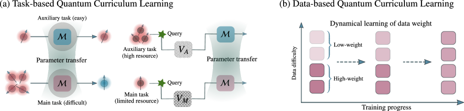
Figure 1: Overview of two principal methodologies in quantum curriculum learning: (a) task-based and (b) data-based approaches. In the task-based approach, a model ${\mathcal{M}}$, designated for a main task that may be challenging or constrained by data accessibility, benefits from pre-training on an auxiliary task. This auxiliary task is either relatively simpler (left panel of (a)) or has a richer dataset (right panel of (a)). In the data-based approach, we implement a dynamic learning schedule to modulate data weights, thereby emphasizing the significance of quantum data in optimizing the loss function to reduce the generalization error.

The typical learning process in QML involves extensive exploration within the domain landscape of a loss function. This function measures the discrepancy between the quantum model’s predictions and the actual values, aiming to locate its minimum using classical computers. However, the optimization often encounters pitfalls such as getting trapped in local minima [15, 16] or barren plateau regions [17]. These scenarios require substantial quantum computational resources to navigate the loss landscape successfully. Additionally, improving task accuracies necessitates evaluating numerous model configurations, especially against extensive datasets. Given the limitation of current quantum resources, this poses a considerable challenge. Therefore, in designing QML models, we must focus not only on their architectural aspects but also on efficient learning strategies.

The perspective of quantum resources refocuses our attention on the concept of learning. In ML, learning refers to the process through which a computer system enhances its performance on a specific task over time by acquiring and integrating knowledge or patterns from data. We can improve current QML algorithms by making this process more efficient. For example, curriculum learning [18] is inspired by the human learning process, based on the intuitive observation that we often begin with simpler concepts before progressing to more complex ones. This insight leads to the development of a strategy for sampling or task scheduling—a curriculum—that introduces simpler samples or tasks to the model before moving on to more challenging ones. Although curriculum learning has been extensively applied and studied in classical ML [19, 20, 21], its exploration in the QML field, especially regarding quantum data, is still in the early stages. The most relevant research has focused on investigating model transfer learning within hybrid classical-quantum neural networks [22]. Typically, this involves starting with a pre-trained classical network that is then modified and enhanced by adding a variational quantum circuit at its final layer. Despite the potential benefits, there is still a lack of concrete evidence that effectively using a curriculum learning framework to schedule tasks and samples improves QML techniques.

In this Letter, we explore the potential of curriculum learning within the context of QML using quantum data. We demonstrate the feasibility of implementing curriculum learning in a quantum framework called quantum curriculum learning (Q-CurL). We consider two common scenarios in training QML models. First, a main task, which may be challenging or limited by data availability, can be facilitated through the preparatory parameter adjustment of an auxiliary task. This auxiliary task is comparatively easier or more data-rich. However, it is necessary to establish the criteria that make an auxiliary task beneficial for a main task. Second, quantum data may carry different weights of importance in the optimization process. Focusing on the partial loss function of difficult data could lead to poorer generalization. We propose two principal approaches for these scenarios: task-based Q-CurL [Fig.1(a)], which determines the curriculum order based on the data density ratio between tasks, and data-based Q-CurL [Fig.1(b)], which employs a dynamic learning schedule that adjusts data weights, thereby prioritizing the importance of quantum data in the optimization. Empirical evidence demonstrates the utility of Q-CurL in enhancing training convergence and generalization when learning unitary dynamics. Furthermore, we show that data-based Q-CurL contributes to increased robustness in learning. Specifically, in scenarios with noisy labels, it can prevent complete memorization of the training data, thereby avoiding overfitting and enhancing generalization performance.

Task-based Q-CurL.— We formulate a framework for task-based Q-CurL. The target of learning is to find a function (or hypothesis, prediction model) $h:{\mathcal{X}}\to{\mathcal{Y}}$ within a hypothesis set ${\mathcal{H}}$ that approximates the true function $f$ mapping ${\bm{x}}\in{\mathcal{X}}$ to ${\bm{y}}=f({\bm{x}})\in{\mathcal{Y}}$ such that $h({\bm{x}})\approx f({\bm{x}})$. To evaluate the correctness of the hypothesis $h$ given the data $({\bm{x}},{\bm{y}})$, the loss function $\ell:{\mathcal{Y}}\times{\mathcal{Y}}\to\mathbb{R}$ is used to measure the approximation error $\ell(h({\bm{x}}),{\bm{y}})$ between the prediction $h({\bm{x}})$ and the target ${\bm{y}}$. We aim to find a hypothesis $h\in{\mathcal{H}}$ that minimizes the expected risk over the distribution $P({\mathcal{X}},{\mathcal{Y}})$:

$$R(h):={\mathbb{E}}_{({\bm{x}},{\bm{y}})\sim P({\mathcal{X}},{\mathcal{Y}})}\left[\ell(h({\bm{x}}),{\bm{y}})\right].$$ (1)

In practice, since the data generation distribution $P({\mathcal{X}},{\mathcal{Y}})$ is unknown, we use the observed dataset ${\mathcal{D}}={({\bm{x}}_{i},{\bm{y}}_{i})}_{i=1}^{N}\subset{\mathcal{X}}\times{\mathcal{Y}}$ to minimize the empirical risk, defined as the average loss over the training data:

$$\hat{R}(h)=\frac{1}{N}\sum_{i=1}^{N}\ell(h({\bm{x}}_{i}),{\bm{y}}_{i}).$$ (2)

Given a main task ${\mathcal{T}}_{M}$, the goal of task-based Q-CurL is to design a curriculum for solving auxiliary tasks to enhance performance compared to solving the main task alone. We consider ${\mathcal{T}}_{1},\ldots,{\mathcal{T}}_{M-1}$ as the set of auxiliary tasks. The training dataset for task ${\mathcal{T}}_{m}$ is ${\mathcal{D}}_{m}\subset{\mathcal{X}}^{(m)}\times{\mathcal{Y}}^{(m)}$ ($m=1,\ldots,M$), containing $N_{m}$ data pairs. We focus on supervised learning tasks with input quantum data ${\bm{x}}^{(m)}_{i}$ in the input space ${\mathcal{X}}^{(m)}$ and corresponding target quantum data ${\bm{y}}^{(m)}_{i}$ in the output space ${\mathcal{Y}}^{(m)}$ for $i=1,\ldots,N_{m}$. The training data $\left({\bm{x}}^{(m)}_{i},{\bm{y}}^{(m)}_{i}\right)$ for task ${\mathcal{T}}_{m}$ are drawn from the probability distribution $P^{(m)}({\mathcal{X}}^{(m)},{\mathcal{Y}}^{(m)})$ with the density $p^{(m)}({\mathcal{X}}^{(m)},{\mathcal{Y}}^{(m)})$. We assume that all tasks share the same data spaces ${\mathcal{X}}^{(m)}\equiv{\mathcal{X}}$ and ${\mathcal{Y}}^{(m)}\equiv{\mathcal{Y}}$, as well as the same hypothesis $h$ and loss function $\ell$ for all $m$.

Depending on the problem, we can decide the curriculum weight $c_{M,m}$, where a larger $c_{M,m}$ indicates a greater benefit of solving ${\mathcal{T}}_{m}$ for improving the performance on ${\mathcal{T}}_{M}$. We evaluate the contribution of solving task ${\mathcal{T}}_{i}$ to the main task ${\mathcal{T}}_{M}$ by transforming the expected risk of training ${\mathcal{T}}_{M}$ as follows:

$$R_{T_{M}}(h) ={\mathbb{E}}_{({\bm{x}},{\bm{y}})\sim P^{(M)}}\left[\ell(h({\bm{x}}),{\bm{y}})\right]$$

$$={\mathbb{E}}_{({\bm{x}},{\bm{y}})\sim P^{(m)}}\left[\dfrac{p^{(M)}({\bm{x}},{\bm{y}})}{p^{(m)}({\bm{x}},{\bm{y}})}\ell(h({\bm{x}}),{\bm{y}})\right].$$ (3)

The curriculum weight $c_{M,m}$ can be determined using the density ratio $r({\bm{x}},{\bm{y}})=\dfrac{p^{(M)}({\bm{x}},{\bm{y}})}{p^{(m)}({\bm{x}},{\bm{y}})}$ without requiring the density estimation of $p^{(M)}({\bm{x}},{\bm{y}})$ and $p^{(m)}({\bm{x}},{\bm{y}})$. The key idea is to model $r({\bm{x}},{\bm{y}})$ using a linear model $\hat{r}({\bm{x}},{\bm{y}}):={\bm{\alpha}}^{\top}{\bm{\phi}}({\bm{x}},{\bm{y}})=\sum_{i=1}^{N_{M}}\alpha_{i}\phi_{i}({\bm{x}},{\bm{y}}),$ where the vector of basis functions is ${\bm{\phi}}({\bm{x}},{\bm{y}})=(\phi_{1}({\bm{x}},{\bm{y}}),\ldots,\phi_{N_{M}}({\bm{x}},{\bm{y}}))$, and the parameter vector ${\bm{\alpha}}=(\alpha_{1},\ldots,\alpha_{N_{M}})^{\top}$ is learned from data [23].

The key factor that differentiates this framework from classical curriculum learning is the consideration of quantum data for ${\bm{x}}$ and ${\bm{y}}$, which are assumed to be in the form of density matrices representing quantum states. Therefore, the basis function $\phi_{l}({\bm{x}},{\bm{y}})$ is naturally defined as the product of global fidelity quantum kernels used to compare two pairs of input and output quantum states as $\phi_{l}({\bm{x}},{\bm{y}})=\operatorname{\textup{Tr}}[{\bm{x}}{\bm{x}}^{(M)}_{l}]\operatorname{\textup{Tr}}[{\bm{y}}{\bm{y}}^{(M)}_{l}].$ In this way, $R_{T_{M}}(h)$ can be approximated as:

$$R_{T_{M}}(h)\approx\dfrac{1}{N_{m}}\sum_{i=1}^{N_{m}}\hat{r}_{\bm{\alpha}}({\bm{x}}^{(m)}_{i},{\bm{y}}^{(m)}_{i})\ell(h({\bm{x}}^{(m)}_{i}),{\bm{y}}^{(m)}_{i}).$$ (4)

The parameter vector ${\bm{\alpha}}$ is estimated via the problem of minimizing $\dfrac{1}{2}{\bm{\alpha}}^{\top}{\bm{H}}{\bm{\alpha}}-{\bm{h}}^{\top}{\bm{\alpha}}+\dfrac{\lambda}{2}{\bm{\alpha}}^{\top}{\bm{\alpha}},$ where we consider the regularization coefficient $\lambda$ for $L_{2}$-norm of ${\bm{\alpha}}$. Here, ${\bm{H}}$ is the $N_{M}\times N_{M}$ matrix with elements $H_{ll^{\prime}}=\dfrac{1}{N_{m}}\sum_{i=1}^{N_{m}}\phi_{l}({\bm{x}}_{i}^{(m)},{\bm{y}}_{i}^{(m)})\phi_{l^{\prime}}({\bm{x}}_{i}^{(m)},{\bm{y}}_{i}^{(m)})$, and ${\bm{h}}$ is the $N_{M}$-dimensional vector with elements $h_{l}=\frac{1}{N_{M}}\sum_{i=1}^{N_{M}}\phi_{l}({\bm{x}}_{i}^{(M)},{\bm{y}}_{i}^{(M)})$.

We consider each $\hat{r}({\bm{x}}^{(m)}_{i},{\bm{y}}^{(m)}_{i})$ as the contribution of the data $({\bm{x}}^{(m)}_{i},{\bm{y}}^{(m)}_{i})$ from the auxiliary task ${\mathcal{T}}_{m}$ to the main task ${\mathcal{T}}_{M}$. We define the curriculum weight $c_{M,m}$ as (see [23] for more details):

$$c_{M,m}=\dfrac{1}{N_{m}}\sum_{i=1}^{N_{m}}\hat{r}_{\bm{\alpha}}({\bm{x}}^{(m)}_{i},{\bm{y}}^{(m)}_{i}).$$ (5)

We consider the unitary learning task to demonstrate the curriculum criteria based on $c_{M,m}$. We aim to optimize the parameters ${\bm{\theta}}$ of a $Q$-qubit parameterized quantum circuit $U({\bm{\theta}})$, such that, for the optimized parameters ${\bm{\theta}}_{\textrm{opt}}$, $U({\bm{\theta}}_{\textrm{opt}})$ can approximate an unknown $Q$-qubit unitary $V$ ($U,V\in\mathcal{U}(\mathbb{C}^{2^{Q}})$).

Our goal is to minimize the Hilbert-Schmidt (HS) distance between $U({\bm{\theta}})$ and $V$, defined as $C_{\textrm{HST}}({\bm{\theta}}):=1-\dfrac{1}{d^{2}}|\operatorname{\textup{Tr}}[V^{\dagger}U({\bm{\theta}})]|^{2},$ where $d=2^{Q}$ is the dimension of the Hilbert space. In the QML-based approach, we can access a training data set consisting of input-output pairs of pure $Q$-qubit states ${\mathcal{D}}_{{\mathcal{Q}}}(N)=\{(\ket{\psi}_{j},V\ket{\psi}_{j})\}_{j=1}^{N}$ drawn from the distribution ${\mathcal{Q}}$. If we take ${\mathcal{Q}}$ as the Haar distribution, we can instead train using the empirical loss:

$$C_{{\mathcal{D}}_{{\mathcal{Q}}}(N)}({\bm{\theta}}):=1-\dfrac{1}{N}\sum_{j=1}^{N}|\braket{\psi_{j}}{V^{\dagger}U({\bm{\theta}})}{\psi_{j}}|^{2}.$$ (6)

The parameterized ansatz unitary $U({\bm{\theta}})$ can be modeled as $U({\bm{\theta}})=\prod_{l=1}^{L}U^{(l)}({\bm{\theta}}_{l})$, consisting of $L$ repeating layers of unitaries. Each layer $U^{(l)}({\bm{\theta}}_{l})=\prod_{k=1}^{K}\exp{(-i\theta_{lk}H_{k})}$ is composed of $K$ unitaries, where $H_{k}$ are Hermitian operators, ${\bm{\theta}}_{l}$ is a $K$-dimensional vector, and ${\bm{\theta}}=\{{\bm{\theta}}_{1},\ldots,{\bm{\theta}}_{L}\}$ is the $LK$-dimensional parameter vector.

We present a benchmark of Q-CurL for learning the approximation of the unitary dynamics of the spin-1/2 XY model with the Hamiltonian $H_{XY}=\sum_{j=1}^{Q}\left(\sigma_{j}^{x}\sigma_{j+1}^{x}+\sigma_{j}^{y}\sigma_{j+1}^{y}+h_{j}\sigma_{j}^{z}\right)$, where $h_{j}\in{\mathbb{R}}$ and $\sigma_{j}^{x},\sigma_{j}^{y},\sigma_{j}^{z}$ are the Pauli operators acting on qubit $j$. This model is important in the study of quantum many-body physics, as it provides insights into quantum phase transitions and the behavior of correlated quantum systems.

To create the main task ${\mathcal{T}}_{M}$ and auxiliary tasks, we represent the time evolution of $H_{XY}$ via the ansatz $V_{XY}$, which is similar to the Trotterized version of $\exp(-i\tau H_{XY})$ [12]. The target unitary for the main task, $V^{(M)}_{XY}=\prod_{l=1}^{L_{M}}V^{(l)}(\bm{\beta}_{l})\prod_{l=1}^{L_{F}}V^{(l)}_{\textrm{fixed}}$, consists of $L_{M}=20$ repeating layers, where each layer $V^{(l)}(\bm{\beta}_{l})$ includes parameterized z-rotations RZ (with assigned parameter $\bm{\beta}_{l}$) and non-parameterized nearest-neighbor $\sqrt{i\textup{SWAP}}=\exp(\frac{i\pi}{8}(\sigma_{j}^{x}\sigma_{j+1}^{x}+\sigma_{j}^{y}\sigma_{j+1}^{y}))$ gates. Additionally, we include the fixed-depth unitary $\prod_{l=1}^{L_{F}}V^{(l)}_{\textrm{fixed}}$ with $L_{F}=20$ layers at the end of the circuit $V^{(l)}$ to increase expressivity. Similarity, keeping the same ${\bm{\beta}}_{l}$, we create the target unitary for the auxiliary tasks ${\mathcal{T}}_{m}$ as $V^{(m)}_{XY}=\prod_{l=1}^{L_{m}}V^{(l)}({\bm{\beta}}_{l})\prod_{l=1}^{L_{F}}V^{(l)}_{\textrm{fixed}}$, with $L_{m}=1,2,\ldots,19$.

Figure 2(a) depicts the average HS distance over 100 trials of ${\bm{\beta}}_{l}$ and $V^{(l)}_{\textrm{fixed}}$ between the target unitary of each auxiliary task ${\mathcal{T}}_{m}$ (with $L_{m}$ layers) and the main task ${\mathcal{T}}_{M}$. We also plot the curriculum weight $c_{M,m}$ in Fig. 2(a) calculated in Eq. (5). Here, we consider the unitary $V_{XY}$ learning with $Q=4$ qubits via the hardware efficient ansatz $U_{\textrm{HEA}}({\bm{\theta}})$  [24, 23] and use $N=20$ Haar random states for input data ${\bm{x}}_{i}^{(m)}$ in each task ${\mathcal{T}}_{m}$. As depicted in Fig. 2(a), $c_{M,m}$ can capture the similarity between two tasks, as higher weights imply smaller HS distances.

Next, we propose a Q-CurL game to further examine the effect of Q-CurL. In this game, Alice has an ML model ${\mathcal{M}}({\bm{\theta}})$ to solve the main task ${\mathcal{T}}_{M}$, but she needs to solve all the auxiliary tasks ${\mathcal{T}}_{1},\ldots,{\mathcal{T}}_{M-1}$ first. We assume the data forgetting in task transfer, meaning that after solving task $A$, only the trained parameters ${\bm{\theta}}_{A}$ are transferred as the initial parameters for task $B$. We propose the following greedy algorithm to decide the curriculum order ${\mathcal{T}}_{i_{1}}\to{\mathcal{T}}_{i_{2}}\to\ldots\to{\mathcal{T}}_{i_{M}=M}$ before training. Starting ${\mathcal{T}}_{i_{M}}$, we find the auxiliary task ${\mathcal{T}}_{i_{M-1}}$ ($i_{M-1}\in\{1,2,\ldots,M-1\}$) with the highest curriculum weights $c_{i_{M},i_{M-1}}$. Similarity, to solve ${\mathcal{T}}_{i_{M-1}}$, we find the corresponding auxiliary task ${\mathcal{T}}_{i_{M-2}}$ in the remaining tasks with the highest $c_{i_{M-1},i_{M-2}}$, and so on. Here, curriculum weights $c_{i_{k},i_{k-1}}$ are calculated similarly to Eq. (5).

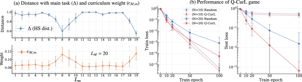
Figure 2: (a) The curriculum weight (lower panel) and the Hilbert-Schmidt distance (upper panel) between the target unitary of the main task ${\mathcal{T}}_{M}$ and the target unitary of the auxiliary task ${\mathcal{T}}_{m}$. (b) The training loss and test loss for different training epochs and different numbers $N$ of training data in the Q-CurL game, considering both random and Q-CurL orders. The average and standard deviations are calculated over 100 trials.

Figure 2(b) depicts the training and test loss of the main task ${\mathcal{T}}_{M}$ (see Eq. (6)) for different training epochs and numbers of training data over 100 trials of parameters’ initialization. In each trial, $N$ Haar random states are used for training, and 20 Haar random states are used for testing. With a sufficient amount of training data ($N=20$), introducing Q-CurL can significantly improve the trainability (lower training loss) and generalization (lower test loss) when compared with random order in Q-CurL game. Even with a limited amount of training data ($N=10$), when overfitting occurs, Q-CurL still performs better than the random order.

Data-based Q-CurL.— We present a form of data-based Q-CurL that dynamically predicts the easiness of each sample at each training epoch, such that easy samples are emphasized with large weights during the early stages of training and conversely. Apart from improving generalization, the benefit of data-based Q-CurL lies in its resistance to noise, which is especially needed in QML. Existing QML models can accurately fit partially corrupted labels to quantum states in the training data but fail on the test data [25]. We show that data-based Q-CurL can enhance the robustness based on the dynamic weighting of the difficulty fitting quantum data to corrupted labels.

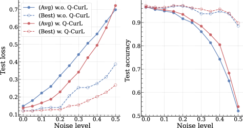
Figure 3: The test loss and accuracy of the trained QCNN (with and without using the data-based Q-CurL) in the quantum phase recognition task with 8 qubits under varying noise levels in corrupted labels. Here, the average and the best performance over 50 trials are plotted.

Inspired by the confidence-aware techniques in classical ML [19, 20, 21], the idea is to modify the empirical risk as

$$\hat{R}(h,{\bm{w}})=\dfrac{1}{N}\sum_{i=1}^{N}\left((\ell_{i}-\eta)e^{w_{i}}+\gamma w^{2}_{i}\right).$$ (7)

Here, ${\bm{w}}=(w_{1},\ldots,w_{N})$, $\ell_{i}=\ell(h({\bm{x}}_{i}),{\bm{y}}_{i})$, and $w^{2}_{i}$ is the regularization term controlled by the hyper-parameter $\gamma>0$. The threshold $\eta$ distinguishes easy and hard samples with $e^{w_{i}}$ emphasizing the loss $l_{i}\ll\eta$ (easy sample) and neglecting the loss $l_{i}\gg\eta$ (hard samples, such as data with corrupted labels). The minimization problem is reduced to $\textup{min}_{{\bm{\theta}}}\textup{min}_{{\bm{w}}}\hat{R}(h,{\bm{w}})$, where ${\bm{\theta}}$ is the parameter of the hypothesis $h$. Here, $\textup{min}_{{\bm{w}}}\hat{R}(h,{\bm{w}})$ is decomposed at each loss $\ell_{i}$ and solved without quantum resources as $w_{i}=\textup{argmin}_{w}(l_{i}-\eta)e^{w}+\gamma w^{2}$. To control the difficulty of the samples, in each training epoch, we set $\eta$ as the average value of all $\ell_{i}$ obtained from the previous epoch. Therefore, $\eta$ changes dynamically during the early stages of training but remains almost constant during the convergence periods.

We apply the data-based Q-CurL to the quantum phase recognition task investigated in Ref. [10] to demonstrate that it can improve the generalization of the learning model. Here, we consider a one-dimensional cluster Ising model with open boundary conditions, whose Hamiltonian with $Q$ qubits is given by $H=-\sum_{j=1}^{Q-2}\sigma^{z}_{j}\sigma^{x}_{j+1}\sigma^{z}_{j+2}-h_{1}\sum_{j=1}^{Q}\sigma^{x}_{j}-h_{2}\sum_{j=1}^{Q-1}\sigma^{x}_{j}\sigma^{x}_{j+1}.$ Depending on the coupling constants $(h_{1},h_{2})$, the ground state wave function of this Hamiltonian can exhibit multiple states of matter, such as the symmetry-protected topological phase, the paramagnetic state, and the anti-ferromagnetic state. We employ the quantum convolutional neural network (QCNN) model [10] with binary cross-entropy loss for training. Without Q-CurL, we use the conventional loss $\hat{R}(h)=(1/N)\sum_{i=1}^{N}\ell_{i}$ for the training and test phase. In data-based Q-CurL, we train the QCNN with the loss $\hat{R}(h,{\bm{w}})$ while using $\hat{R}(h)$ to evaluate the generalization on the test data set. We use 40 and 400 ground state wave functions for the training and test phase, respectively (see [23] for details of settings).

To evaluate the effectiveness of the data-based Q-CurL in considering the difficulty of the data in training, we consider the scenario of fitting corrupted labels. Given a probability $p$ ($0\leq p\leq 1$) representing the noise level, the true label $y_{i}\in\{0,1\}$ of training state $\ket{\psi_{i}}$ is transformed to the label $1-y_{i}$ with probability $p$, while it remains the true label with probability $1-p$. Figure 3 illustrates the performance of trained QCNN on test data across different noise levels. There is no significant difference at low noise levels, but as the noise level increases, the conventional training fails to generalize effectively. In this case, introducing data-based Q-CurL in training (red lines) reduces the test loss and enhances testing accuracy compared to the conventional method (blue lines).

Discussion.— The proposed Q-CurL framework can enhance training convergence and generalization in QML with quantum data. Future research should investigate whether Q-CurL can be designed to improve trainability in QML, particularly by avoiding the barren plateau problem. For instance, curriculum design is not limited to tasks and data but can also involve the progressive design of the loss function. Even when the loss function of the target task, designed for infeasibility in classical simulation to achieve quantum advantage [26, 27], is prone to the barren plateau problem, a well-designed sequence of classically simulable loss functions can be beneficial. Optimizing these functions in a well-structured curriculum before optimizing the main function may significantly improve the trainability and performance of the target task.