The Symplectic Schur Process

Abstract

We define a measure on tuples of partitions, called the symplectic Schur process, that should be regarded as the right analogue of the Schur process of Okounkov-Reshetikhin for the Cartan type C. The weights of our measure include factors that are universal symplectic characters, as well as a novel family of “Down-Up Schur functions” that we define and for which we prove new identities of Cauchy-Littlewood-type. Our main structural result is that the point process corresponding to the symplectic Schur process is determinantal and we find an explicit correlation kernel. We also present dynamics that preserve the family of symplectic Schur processes and explore an alternative sampling scheme, based on the Berele insertion algorithm, in a special case. Finally, we study the asymptotics of the Berele insertion process and find explicit formulas for the limit shape and fluctuations near the bulk and the edge. One of the limit regimes leads to a new kernel that resembles the symmetric Pearcey kernel.

To the memory of Anatoly Moiseevich Vershik, with admiration.

1 Introduction

1.1 Background

In their seminal paper [OR-2003], Okounkov and Reshetikhin introduced the Schur process, a probability measure on the set of tuples of integer partitions

$$\varnothing\subset\lambda^{(1)}\supset\mu^{(1)}\subset\cdots\subset\lambda^{(k-1)}\supset\mu^{(k-1)}\subset\lambda^{(k)}\supset\varnothing,$$

of the form

$$\mathbb{P}^{\text{SP}}\!\left(\vec{\lambda},\vec{\mu}\,\big{|}\,\vec{\mathbf{x}},\vec{\mathbf{y}}\right)\propto s_{\lambda^{(1)}}(\mathbf{x}^{1})\,s_{\lambda^{(1)}/\mu^{(1)}}(\mathbf{y}^{1})\,s_{\lambda^{(2)}/\mu^{(1)}}(\mathbf{x}^{2})\,\cdots\\ \cdots\,s_{\lambda^{(k-1)}/\mu^{(k-1)}}(\mathbf{y}^{k-1})\,s_{\lambda^{(k)}/\mu^{(k-1)}}(\mathbf{x}^{k})\,s_{\lambda^{(k)}}(\mathbf{y}^{k}),$$ (1.1)

where $s_{\lambda}$ (resp. $s_{\lambda/\mu}$) are the Schur functions (resp. skew Schur functions) and $\mathbf{x}^{1},\dots,\mathbf{x}^{k}$, $\mathbf{y}^{1},\dots,\mathbf{y}^{k}$ are sets of variables. Since its introduction, this measure has been the object of constant attention due to its ubiquitous nature and applications in the asymptotic analysis of random growth processes [BF-2014], line ensembles [CH-2014], random tilings [Gor-2021], asymptotic representation theory [Bor-2011], Gromov-Witten invariants [OP-2006], topological string theory [ORV-2006], among others. The Schur process combines the desirable properties of being amenable to very precise combinatorial and asymptotic analysis and of being a good mathematical model to describe a large variety of physical phenomena involving randomly interacting particles. In fact, the existence itself of the Schur process as an example of a completely solvable model of randomly interacting bodies has been one of the catalysts of the success of Integrable Probability; e.g. see the survey [BG-2016].

The Schur polynomials, which are the fundamental building block of the Schur process, have notable representation theoretic interpretations. For example, they are (i) the characters of the irreducible representations for the symmetric group (under the characteristic isometry) and (ii) the characters of the polynomial irreducible representations for the general linear groups or unitary groups. Another connection with representation theory comes by looking at the marginals of the Schur process, which are the Schur measures, introduced earlier by Okounkov [Ok-2001b], based on the Cauchy identity:

$$\sum_{\lambda}s_{\lambda}(x_{1},\dots,x_{n})s_{\lambda}(y_{1},\dots,y_{m})=\prod_{i=1}^{n}\prod_{j=1}^{m}\frac{1}{1-x_{i}y_{j}}.$$ (1.2)

The identity (1.2) itself is a manifestation of the Howe duality for the action of the pair of Lie groups $(GL(n),GL(m))$ on $\mathrm{Sym}(\mathbb{C}^{n}\otimes\mathbb{C}^{m})$. Additionally, it is known that the Schur measures generalize the $z$-measures that arise as the solution to the problem of noncommutative harmonic analysis for the infinite symmetric group $S(\infty)$ and, in fact, this was the original motivation for their definition, see e.g. [BO-2017, Ok-2001a]. As a result of the previous observations, the Schur measure and Schur process should be regarded as objects associated to the Cartan type $A$, since they are related to the symmetric and general linear groups. Naturally, there exist canonical analogs of some of the above algebraic structures for “other symmetry types”, and some of the corresponding probability measures have already been considered in the literature, e.g. [NOS-2024] studies probability measures associated to skew-Howe dualities, [CG-2020] considers measures arising from the branching rule of symplectic Schur polynomials with $q$-specializations, etc.

We will work here with the symplectic Schur polynomials $\text{sp}_{\lambda}(x_{1}^{\pm},\dots,x_{n}^{\pm})$, which are characters of the irreducible representations of the symplectic Lie group $Sp(2n)$ [King-1975]. Alternatively, they can be defined by the summation identity [Lit-1950, Weyl-1946]

$$\sum_{\lambda:\,\ell(\lambda)\leq n}\text{sp}_{\lambda}(x_{1}^{\pm},\dots,x_{n}^{\pm})s_{\lambda}(y_{1},\dots,y_{n})=\frac{\prod_{1\leq i<j\leq n}(1-y_{i}y_{j})}{\prod_{i,j=1}^{n}(1-y_{j}x_{i})(1-y_{j}/x_{i})},$$ (1.3)

usually referred to as Cauchy-Littlewood identity, which is a consequence of the duality between irreducible finite-dimensional representations of the compact symplectic group $Sp(2n)$ and irreducible infinite-dimensional unitary highest weight representations of the non-compact Lie group $SO^{*}(2n)$, a real form of the complex orthogonal group [Howe-1989, KV-1978]. The symplectic Schur polynomials $\text{sp}_{\lambda}(x_{1}^{\pm},\dots,x_{n}^{\pm})$ are Laurent polynomials in the variables $x_{1},\dots,x_{n}$ and, on top of their representation theoretic interpretation, they also possess interesting combinatorial intepretations. For instance, they are generating functions of a class of semi-standard tableaux called symplectic tableaux [King-1975] (see Section 7 below) or of Kashiwara-Nakashima tableaux [KN-1994].

Since all terms of the left hand side summation are nonnegative (provided we let $x_{i},y_{i}>0$), it is tempting to use (1.3) to define a probability measure on integer partitions as a symplectic variant of the Schur measure. This was done in [Bet-2018], where it was found that such a measure defines a determinantal point process with an explicit correlaton kernel. In the same paper, Betea carried out the asymptotic analysis for the case when one considers that the specializations in the identity (1.3) are Plancherel, and showed that the result is a signed measure with the physically interesting kernel $\text{Airy}_{2\to 1}$ arising in certain limit regime.

In this paper we define the symplectic Schur process as a natural analog of (1.1), having marginal distributions given by the symplectic Schur measure from [Bet-2018]. This construction is not canonical and is far from straightforward because of two main factors:

(i) The symplectic Schur polynomials have a non-trivial branching structure and the skew polynomials $\text{sp}_{\lambda/\mu}$ depend on the number of zeroes that $\lambda$ and $\mu$ have appended at the end. We avoid this complication by considering symmetric functions; it turns out that the $\text{sp}_{\lambda/\mu}$ turn into the skew Schur functions $s_{\lambda/\mu}$ when infinitely many variables are considered, see equation (1.4). We also need to define new symmetric functions $T_{\lambda,\mu}$ that are skew-dual to $\text{sp}_{\lambda/\mu}$ and will be called the down-up Schur functions.

(ii) Summations identities such as (1.3) for skew variants of sp are not well-established in the literature with the exception of a particular variant recently found in [JLW-2024]. In fact, the understanding of that paper from the point of view of symmetric functions was the origin of the present article.

1.2 Main results

1.2.1 Universal symplectic characters

Following [KT-1987], define the universal symplectic characters through the following determinant of Jacobi-Trudi type:

$$\text{SP}_{\lambda}(x)=\frac{1}{2}\cdot\det_{1\leq i,j\leq\ell(\lambda)}\left[h_{\lambda_{i}-i+j}(x)+h_{\lambda_{i}-i-j+2}(x)\right].$$

Above, the $h_{k}$’s are the complete homogeneous symmetric functions. When $x$ is the finite collection of variables $(x_{1},x_{1}^{-1},\dots,x_{n},x_{n}^{-1})$ and $n\geq\ell(\lambda)$, this object reduces to the symplectic Schur polynomial

$$\text{SP}_{\lambda}(x_{1},x_{1}^{-1},\dots,x_{n},x_{n}^{-1})=\text{sp}_{\lambda}(x_{1}^{\pm},\dots,x_{n}^{\pm}),\quad\text{for }\ell(\lambda)\leq n,$$

and thus carries the information about the characters of irreducible representations of $Sp(2n)$.

For the universal symplectic characters, we prove in 3.8 the branching rule

$$\text{SP}_{\lambda}(x,y)=\sum_{\mu}\text{SP}_{\mu}(x)s_{\lambda/\mu}(y),$$ (1.4)

which, to the best of our knowledge, is new. In light of the combinatorial interpretation of the symplectic Schur polynomials, the branching rule (1.4) looks counter-intuitive. In fact, the definition of $\text{sp}_{\lambda}(x_{1}^{\pm},\dots,x_{n}^{\pm})$ as the generating function of symplectic tableaux of shape $\lambda$ gives rise to an alternative branching formula, which for partitions $\lambda$, such that $\ell(\lambda)\leq n$, reads

$$\text{sp}_{\lambda}(x_{1}^{\pm},\dots,x_{n-k}^{\pm},y_{1}^{\pm},\dots,y_{k}^{\pm})=\sum_{\mu=(\mu_{1},\dots,\mu_{n-k})}\text{sp}_{\mu}(x_{1}^{\pm},\dots,x_{n-k}^{\pm})\,\text{sp}_{\lambda/\mu}(y_{1}^{\pm},\dots,y_{k}^{\pm}),$$ (1.5)

where the branching factors $\text{sp}_{\lambda/\mu}(y_{1}^{\pm},\dots,y_{k}^{\pm})$ are generating functions of certain symplectic skew-tableaux. Rather recently, the branching structure (1.5) was studied in [JLW-2024, AFHSA-2023], where explicit determinantal formulas of Jacobi-Trudi type for $\text{sp}_{\lambda/\mu}$ were found. The important caveat to differentiate between the two (apparently contradictory) expressions (1.4) and (1.5) is that, while the summation in (1.4) ranges over all partitions, that of (1.5) ranges over partitions $\mu$ of length bounded by $n-k$. Another difference is that the specializations in (1.4) are more general than the specific variable specializations in (1.5); this is the first indication that working with generic specializations will indeed simplify the symmetric function identities needed for our purposes. In principle, it should in fact be possible to derive (1.5) from (1.4), although we will not attempt this.

1.2.2 Down-up Schur functions and skew Cauchy-Littlewood identities

We define a family of symmetric functions $T_{\lambda,\mu}$, parametrized by two partitions $\lambda,\mu$, which we will call the down-up Schur functions, as

$$T_{\lambda,\mu}(y)=\sum_{\nu}d_{\mu,\nu}^{\lambda}s_{\nu}(y),$$ (1.6)

where $d_{\mu,\nu}^{\lambda}$ are the Newell-Littlewood (NL) coefficients [Lit-1958, New-1951]. These coefficients are “symplectic analogs” of the Littlewood-Richardson coefficients, as they compute the multiplicity of an irreducible representation in the decomposition of tensor products of irreducible representations of the symplectic group: this can be expressed in terms of symmetric polynomials by the expansion

$$\text{sp}_{\mu}(x_{1}^{\pm},\dots x_{n}^{\pm})\,\text{sp}_{\nu}(x_{1}^{\pm},\dots x_{n}^{\pm})=\sum_{\lambda:\,\ell(\lambda)\leq n}d^{\lambda}_{\mu,\nu}\,\text{sp}_{\lambda}(x_{1}^{\pm},\dots x_{n}^{\pm}),$$

valid for $\ell(\mu)+\ell(\nu)\leq n$, see [KT-1987, GOY-2021]. To the best of our knowledge, the functions $T_{\lambda,\mu}$ have not been defined in literature until now, although the NL coefficients are well-known. Notable properties of the NL coefficients allow to express the symmetric function $T_{\lambda,\mu}$ as (see 4.2)

$$T_{\lambda,\mu}(y)=\sum_{\kappa}s_{\lambda/\kappa}(y)s_{\mu/\kappa}(y),$$ (1.7)

which motivates the name we adopted. The expression (1.7) can be used, along with summation formulas for skew Schur polynomials, to derive the following branching rule (see 4.4)

$$\sum_{\lambda}T_{\rho,\lambda}(y)T_{\lambda,\mu}(z)=\frac{T_{\rho,\mu}(y,z)}{\prod_{i,j}(1-y_{i}z_{j})}.$$

The main motivation to introduce the down-up Schur functions is that they are skew-duals with respect to the universal symplectic characters, in the sense that they satisfy the following variant of the Cauchy-Littlewood identity

$$\sum_{\nu}\text{SP}_{\nu}(x)T_{\lambda,\nu}(y)=\frac{\prod_{i<j}(1-y_{i}y_{j})}{\prod_{i,j}(1-x_{i}y_{j})}\,\text{SP}_{\lambda}(x).$$

Moreover, we prove the following skew down-up Cauchy identity (see 4.5)

$$\sum_{\rho}{s_{\rho/\mu}(y)T_{\rho,\lambda}(z)}=\frac{1}{\prod_{i,j}(1-y_{i}z_{j})}\sum_{\eta}{s_{\lambda/\eta}(y)T_{\mu,\eta}(z)},$$

which is instrumental for our probabilitstic applications.

Recently, skew dual variants of symplectic Schur polynomials were identified by Jing-Li-Wang, who constructed them in [JLW-2024] using the formalism of vertex operators. This construction expresses $T_{\lambda,\nu}(y_{1},\dots,y_{n})$, there called $S^{*}_{\lambda/\nu}(y_{1},\dots,y_{n})$, in terms of a Weyl-type determinant with the result being a priori a Laurent polynomial with no precise combinatorial description. We believe that our symmetric function definition (1.6), or equivalently (1.7), provides more insights into the combinatorial and algebraic nature of the symmetric functions $T_{\lambda,\nu}$.

1.2.3 The symplectic Schur process

Having discussed the necessary notions from symmetric functions in the previous subsections, we can introduce the main object of this paper. We define the symplectic Schur process as the measure on (pairs of) sequences of partitions $\vec{\lambda}=(\lambda^{(1)},\dots,\lambda^{(k)})$, $\vec{\mu}=(\mu^{(1)},\dots,\mu^{(k-1)})$, defined by

$$\mathbb{P}^{\text{SSP}}\!\left(\vec{\lambda},\vec{\mu}\,\big{|}\,\vec{\mathcal{A}},\vec{\mathcal{B}}\right):=\frac{1}{Z(\vec{\mathcal{A}},\vec{\mathcal{B}})}\cdot s_{\lambda^{(1)}}(\mathcal{B}^{1})\cdot\prod_{j=1}^{k-1}{\left[s_{\lambda^{(j)}/\mu^{(j)}}(\mathcal{A}^{j})\,T_{\mu^{(j)},\lambda^{(j+1)}}(\mathcal{B}^{j+1})\right]}\cdot\text{SP}_{\lambda^{(k)}}(\mathcal{A}^{k}),$$ (1.8)

where $\mathcal{A}^{1},\dots\mathcal{A}^{k},\mathcal{B}^{1},\dots,\mathcal{B}^{k}$ are specializations of the algebra of symmetric functions (see 5.1). Moreover, $Z(\vec{\mathcal{A}},\vec{\mathcal{B}})$ is the normalization constant that makes the total mass of the measure equal to $1$. A closed formula for $Z(\vec{\mathcal{A}},\vec{\mathcal{B}})$ can be computed through the use of identities of the Cauchy-Littlewood-type; see 5.8. The reader should compare our definintion with the equation (1.1) that defines the Schur process. Note that the support of the symplectic Schur process consists of tuples $(\vec{\lambda},\vec{\mu})$ such that $\mu^{(j)}\subseteq\lambda^{(j)}$, for all $1\leq j\leq k-1$, but unlike the Schur process, the containments $\mu^{(j)}\subseteq\lambda^{(j+1)}$ are not necessarily true; see Figure 1 for a representation of the support.

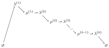
Figure 1: Representation of the support of the symplectic Schur process.

As a (possibly signed) measure, we prove that the symplectic Schur process is a determinantal point process. To state this result precisely, consider for each pair $(\vec{\lambda},\vec{\mu})$ the point configuration $\mathcal{L}(\vec{\lambda},\vec{\mu})$ on the space $\{1,\frac{3}{2},2,\dots,k-\frac{1}{2},k\}\times\mathbb{Z}$, given by

$$\mathcal{L}(\vec{\lambda},\vec{\mu}):=\left\{\left(1,\,\lambda^{(1)}_{i}-i\right)\right\}_{i\geq 1}\cup\left\{\left(\frac{3}{2},\,\mu^{(1)}_{i}-i\right)\right\}_{i\geq 1}\cup\left\{\left(2,\,\lambda^{(2)}_{i}-i\right)\right\}_{i\geq 1}\cup\ \cdots\\ \cdots\ \cup\left\{\left(k-1,\,\lambda^{(k-1)}_{i}-i\right)\right\}_{i\geq 1}\cup\left\{\left(k-\frac{1}{2},\,\mu^{(k-1)}_{i}-i\right)\right\}_{i\geq 1}\cup\left\{\left(k,\,\lambda^{(k)}_{i}-i\right)\right\}_{i\geq 1}.$$

Theorem 1.1 (See 5.18 in the text).

For any $S\geq 1$ distinct points $(i_{1},u_{1}),\dots,(i_{S},u_{S})$ of $\{1,\frac{3}{2},2,\dots,k-1,k-\frac{1}{2},k\}\times\mathbb{Z}$, we have the following identity

$$\sum_{\{(i_{1},u_{1}),\dots,(i_{S},u_{S})\}\subset\mathcal{L}(\vec{\lambda},\vec{\mu})}{\mathbb{P}^{\text{SSP}}\!\left(\vec{\lambda},\vec{\mu}\,\big{|}\,\vec{\mathcal{A}},\vec{\mathcal{B}}\right)}=\det_{1\leq s,t\leq S}\left[K^{\text{SSP}}(i_{s},u_{s};i_{t},u_{t})\right].$$

The explicit expression of the kernel $K^{\text{SSP}}$ is given in Equation (5.16) as a double contour integral.

Figure 2: A depiction of the point process $\mathcal{L}(\vec{\lambda})$ constructed through Berele insertion.

Remark 1.2.

In analogy with the Schur process, the marginals of the symplectic Schur process are given by the symplectic Schur measure. Moreover, a determinantal correlation kernel for the symplectic Schur measure was found by Betea in [Bet-2018] and corresponds exactly to $K^{\textrm{Betea}}(u,v)=K^{\text{SSP}}(i,u;i,v)$, for $i$ fixed.

For general specializations $\mathcal{A}^{i},\mathcal{B}^{j}$, the symplectic Schur process is a signed measure. It is an important question to classify all specializations for which $\mathbb{P}^{\text{SSP}}$ is a probability measure, i.e. for which the product in the right hand side of (1.8) is nonnegative for every choice of sequences of partitions $\vec{\lambda},\vec{\mu}$. In Section 5.5, we find large families of examples of specializations for which this is the case. We note that this contribution is more difficult than in the case of Schur processes. This boils down to the fact that the classical problem of classification of Schur-positive specializations, i.e. specializations $\mathcal{A}$ such that

$$s_{\lambda/\mu}(\mathcal{A})\geq 0,\qquad\text{for all }\lambda,\mu\in\mathbb{Y},$$

has been solved in 1952 by [Whi-1952, ASW-1952, Edr-1952]. On the other hand, for the universal symplectic character $\text{SP}_{\lambda}$, the existence of positive specializations is not established and, in fact, it is not even clear they exist at all. For instance, in the case when $\mathcal{A}=(x_{1},x_{1}^{-1},\dots,x_{n},x_{n}^{-1})$ with $x_{1},\dots,x_{n}>0$, we have

$$\text{SP}_{\lambda}(x_{1},x_{1}^{-1},\dots,x_{n},x_{n}^{-1})\geq 0,\quad\text{whenever }\ell(\lambda)\leq n,$$

however, if $\ell(\lambda)>n$, we might have $\text{SP}_{\lambda}(x_{1},x_{1}^{-1},\dots,x_{n},x_{n}^{-1})<0$, and the explicit value can even be calculated from the results of [KT-1987]. For instance, if $n=1$ and $\lambda=(1,1,1)$, we have $\text{SP}_{(1,1,1)}(x_{1},x_{1}^{-1})=-2(x_{1}+x_{1}^{-1})$.

1.2.4 Symplectic Schur process through Berele sampling

In Section 6, we present dynamics that preserve the symplectic Schur processes (1.8). One of the dynamics is a growth process that can yield a perfect sampling algorithm for certain specializations. However, we chose to analyze in this article the asymptotics of the following interesting example, that can be alternatively sampled by a process that adds or removes boxes from the partitions at each step. Consider the symplectic Schur process with the following choice of specializations

$\mathcal{A}^{1}=\dots=\mathcal{A}^{k-1}=\varnothing,$  $\mathcal{A}^{k}=(x_{1},x_{1}^{-1},\dots,x_{n},x_{n}^{-1}),$  $\mathcal{B}^{1}=(y_{1}),$ …, $\mathcal{B}^{k}=(y_{k}),$

where $k\leq n$ and $x_{1},\dots,x_{n},y_{1},\dots,y_{k}$ are positive real numbers satisfying $0<x_{i}y_{j},x_{i}^{-1}y_{j}<1$, for all $1\leq i\leq n$, $1\leq j\leq k$. In this case, the symplectic Schur process is a probability measure on $k$-tuples of partitions $\vec{\lambda}=(\lambda^{(1)},\dots,\lambda^{(k)})$ that admits an explicit sampling procedure through the Berele insertion algorithm [Ber-1986], a symplectic version of the Robinson-Schensted-Knuth algorithm; see Section 7.

To construct a random sequence $\vec{\lambda}=(\lambda^{(1)},\dots,\lambda^{(k)})$, one first needs to prepare $k$ random words $w_{1},\dots,w_{k}$ in the alphabet $\mathsf{A}_{n}=\{1,\overline{1},\dots,n,\overline{n}\}$ by setting

$$w_{j}=\underbrace{1\,\cdots\,1}_{m_{1,j}}\underbrace{\overline{1}\,\cdots\,\overline{1}}_{\overline{m}_{1,j}}\,\cdots\,\underbrace{n\,\cdots\,n}_{m_{n,j}}\underbrace{\overline{n}\,\cdots\,\overline{n}}_{\overline{m}_{n,j}},$$

where $m_{i,j},\overline{m}_{i,j}$, counting the number of occurrences of $i,\overline{i}$ in $w_{j}$, are sampled independently with the geometric laws $\mathrm{Geo}(x_{i}y_{j}),\mathrm{Geo}(x_{i}^{-1}y_{j})$, respectively. Then the Berele insertion scheme offers a procedure to insert the words $w_{j}$’s sequentially into an initially empty symplectic Young tableau and obtain the sequence

$$\varnothing\xrightarrow[]{w_{1}}P_{1}\xrightarrow[]{w_{2}}P_{2}\xrightarrow[]{w_{3}}\,\cdots\,\xrightarrow[]{w_{k}}P_{k},$$

whose shapes

$$\lambda^{(1)},\dots,\lambda^{(k)},$$

namely $\lambda^{(j)}=\mathrm{shape}(P_{j})$, follow the law of a symplectic Schur process. This result is contained in 7.5. In Figure 2, we report a sample of the point process $\mathcal{L}(\vec{\lambda}):=\{(j,\,\lambda^{(j)}_{i}-i)\mid i\geq 1,\,j=1,\dots,k\}$, constructed through our Berele insertion process with parameters

$$x_{1}=\cdots=x_{n}=1,\qquad y_{1}=\cdots=y_{k}=1/2.$$ (1.9)

As an application of 1.1, for the special case of the choice of parameters (1.9), we also perform the asymptotic analysis, computing the limit shape for large $k,n$ and identifying the limiting random processes in the bulk and at the edge. These results are elaborated on in Section 8. Like in the case of the Schur process, the limiting processes turn out to be the Airy process at the edge (8.2), a certain extended Sine process in the bulk (8.1) and the GUE corners process on microscopic regions where the limit shape is tangent to frozen regions (8.7).

In Section 8.6, we also consider the asymptotic analysis of the correlation kernel in the regime where $k>n$, in which case the Berele insertion process is no longer described by the symplectic Schur process and where the measure $\mathbb{P}^{\text{SSP}}$ fails in general to be a probability measure. Heuristically, this limit should describe what happens when the tangent point between the liquid region of the limit shape and the horizontal line $[0,+\infty)\times\{-n\}$. It turns out that the asymptotic limit of the kernel $K^{\text{SSP}}$ produces a new kernel, which is a variant of the Pearcey kernel and bears resemblance to the Symmetric Pearcey kernel from [BK-2010]. It is worth mentioning here that the Pearcey kernel and a symmetric variation of it have recently shown up in limits of probability measures arising from the skew $(GL(n),GL(k))$-duality with piecewise-constant and alternating specializations, respectively, [BNNSS-2024+]; it would be interesting to compare these kernels to ours.

1.3 Outlook and future research directions

Since its introduction, numerous generalizations of the Schur process have been proposed. Some of the notable ones are: (a) the periodic Schur process [Bor-2007], a model of cylindric partitions which can be regarded as a Schur process of Cartan type $\hat{A}$ [Tin-2007]; (b) the Macdonald process [BC-2014], which employs Macdonald symmetric functions in place of Schur functions; (c) the Spin Hall-Littlewood processes [BP-2019, BMP-2021, AB-2024] where Schur functions are replaced by symmetric functions originating from partition functions of integrable vertex models.

The list presented above is all but complete. We note that these generalizations also have applications that are unreachable by the Schur process, e.g. to the analysis of $\beta$-Jacobi corners process [BG-2015] and directed polymers [BC-2014]. In general, the presence of branching rules and Cauchy-type identities allows to construct solvable Schur-type processes; other recent examples are [OCSZ-2014, MP-2022, Kos-2021, CGK-2022, GP-2024]. Just like the Schur process, we envision the symplectic variant defined here to be amenable to various generalizations and further applications. A natural one is to lift universal symplectic characters to Macdonald-Koornwinder functions [Rai-2005]. Some initial steps in this direction were taken by [Nte-2016] for $q$-Whittaker polynomials. On the other hand, [WZJ-2016] studied integrable vertex models to prove identities for BC-type Hall-Littlewood polynomials. More recently, stochastic vertex models of symplectic type were defined in [Zho-2022], but their connection to random partitions is unclear.

Another interesting direction includes testing alternative sampling schemes for the symplectic Schur process. Contrary to the case of combinatorics in type $A$, which is largely encompassed by the celebrated RSK correspondence, combinatorics in type $C$ is richer and less straightforward. For instance, the Berele insertion recalled below in Section 7 is not the canonical extension of the RSK correspondence, and other combinatorial correspondences can be put in place to prove the Cauchy-Littlewood identity (see [HK-2022]); they have other desirable properties, such as compatibility with crystal symmetries [Lee-2023]. It would be interesting to investigate sampling schemes based on these other combinatorial correspondences, which would possibly prove fruitful to understand if extensions in affine setting, in the style of [Bor-2007] or connections with solitonic systems [IMS-2023] are possible.

Finally, we mention that the dynamics preserving the symplectic Schur process from Section 6 can lead to various surface growth models; for the construction of similar dynamics that preserve the Schur and Macdonald processes, see [BP-2016, BF-2014] and the survey [BP-2014]. It would be interesting to explore various general schemes for random growth of sequences of partitions and stepped surfaces. Related Markov processes that preserve the BC-type $z$-measures (see [Cue-2018a] and [BO-2005, Sec. 8]) from asymptotic representation theory were constructed in [Cue-2018b].

Acknowledgments

This research was partially funded by the European Union’s Horizon 2020 research and innovation programme under the Marie Skłodowska-Curie grant agreement No. 101030938. C.C. is grateful to Alexei Borodin, Grigori Olshanski and Anton Nazarov for helpful conversations, and to the the University of Warwick for hosting him during the beginning stages of this project.

2 Background on symmetric polynomials and Schur functions

We will assume that the reader is familiar with the language of symmetric functions, e.g. from [Mac-1995, Ch. I]. In this section, we simply recall some definitions and set our notations.

Partitions will be denoted by lowercase Greek letters $\lambda,\mu,\rho$, etc., and they will be identified with their corresponding Young diagrams. The set of all partitions is denoted by $\mathbb{Y}$. For any $\lambda\in\mathbb{Y}$, the size of $\lambda$ is denoted by $|\lambda|$ and set $\mathbb{Y}_{n}:=\{\lambda\in\mathbb{Y}:|\lambda|=n\}$, so that the set of all partitions is $\mathbb{Y}=\bigsqcup_{n\geq 0}{\mathbb{Y}_{n}}$ and includes the empty partition $\varnothing\in\mathbb{Y}_{0}$. Finally, $\ell(\lambda)$ will denote the length of $\lambda$.

2.1 Schur polynomials and their symplectic analogues

Definition 2.1.

Let $n\in\mathbb{Z}_{\geq 0}$ and let $\lambda$ be any partition with $\ell(\lambda)\leq n$.

• For variables $y_{1},\dots,y_{n}$, let $y:=(y_{1},\dots,y_{n})$ and define

  $$s_{\lambda}(y):=\frac{\det_{1\leq i,j\leq n}\left(y_{i}^{\lambda_{j}+n-j}\right)}{\prod_{1\leq i<j\leq n}(y_{i}-y_{j})}.$$

  We call $s_{\lambda}(y)$ a Schur polynomial.

• For variables $x_{1},\dots,x_{n}$, let $x^{\pm}:=(x_{1}^{\pm},\dots,x_{n}^{\pm})=(x_{1},x_{1}^{-1},\dots,x_{n},x_{n}^{-1})$ and define

  $$\text{sp}_{\lambda}(x^{\pm}):=\frac{\det_{1\leq i,j\leq n}\left(x_{i}^{\lambda_{j}+n-j+1}-x_{i}^{-(\lambda_{j}+n-j+1)}\right)}{\prod_{1\leq i<j\leq n}(x_{i}-x_{j})(1-x_{i}^{-1}x_{j}^{-1})\prod_{i=1}^{n}(x_{i}-x_{i}^{-1})}.$$

  We call $\text{sp}_{\lambda}(x^{\pm})$ a symplectic Schur polynomial.

Clearly, $s_{\lambda}(y)$ is a symmetric polynomial in the variables $y_{1},\dots,y_{n}$, homogeneous of degree $|\lambda|$. The Schur polynomials are character values of the irreducible polynomial representations of $GL(n,\mathbb{C})$ evaluated at the maximal torus $\mathbb{T}^{n}:=\{\text{diag}(y_{1},\dots,y_{n}):y_{i}\in\mathbb{C}^{\times}\}$, see e.g. [Weyl-1946].

By contrast, $\text{sp}_{\lambda}(x^{\pm})$ are symmetric Laurent polynomials, i.e. polynomials in $x_{1}^{\pm},\dots,x_{n}^{\pm}$, symmetric with respect to the natural action of the hyperoctahedral group $S_{n}\ltimes(\mathbb{Z}/2\mathbb{Z})^{n}$. The symplectic Schur polynomial $\text{sp}_{\lambda}(x^{\pm})$ can also be expressed as a symmetric polynomial in the variables $x_{1}+x_{1}^{-1},\dots,x_{n}+x_{n}^{-1}$, of degree $|\lambda|$, but inhomogeneous. They are also character values of the irreducible representations of $Sp(2n)$ evaluated at a maximal torus, see e.g. [King-1975].

The following identity will be useful; for proofs, see e.g. [Koi-1989, Sun-1990].

Proposition 2.2 (Cauchy-Littlewood identity for symplectic Schur polynomials).

Let $n\geq k$ be two nonnegative integers, and let $x^{\pm}=(x_{1}^{\pm},\dots,x_{n}^{\pm}),\,y=(y_{1},\dots,y_{k})$. Then

$$\sum_{\mu\,:\,\ell(\mu)\leq k}{\text{sp}_{\mu}(x^{\pm})s_{\mu}(y)}=\frac{\prod_{1\leq i<j\leq k}(1-y_{i}y_{j})}{\prod_{i=1}^{n}\prod_{j=1}^{k}{(1-x_{i}y_{j})(1-x_{i}^{-1}y_{j})}}.$$ (2.1)

The identity (2.1) can be interpreted either as an equality of power series in $\mathbb{C}[[x_{1}+x_{1}^{-1},\dots,x_{n}+x_{n}^{-1},y_{1},\dots,y_{n}]]$, or as a numerical equality when $|y_{j}|<\min\{|x_{i}|,|x_{i}|^{-1}\}$, for all $1\leq i\leq n$, $1\leq j\leq k$ (so that the left hand side is absolutely convergent).

2.2 The algebra of symmetric functions

We denote the graded real algebra of symmetric functions by $\Lambda=\bigoplus_{n\geq 0}{\Lambda_{n}}$, where $\Lambda_{n}$ consists of the homogeneous symmetric functions of degree $n$, and $\Lambda_{0}=\mathbb{R}$. The power sums $p_{1},p_{2},\dots$ are algebraically independent generators of $\Lambda$ with $\deg(p_{n})=n$, for all $n\geq 1$, so that $\Lambda=\mathbb{R}[p_{1},p_{2},\dots]$.

Symmetric functions can be regarded as functions on an infinite set of variables $y_{1},y_{2},\dots$ that are invariant with respect to any finitary permutation of variables, e.g. setting $p_{k}=y_{1}^{k}+y_{2}^{k}+\cdots$. Indeed, let $\mathbb{C}[y_{1},\dots,y_{n}]^{S_{n}}$ be the space of symmetric polynomials in the $n$ variables $y_{1},\dots,y_{n}$ and let $\pi^{n+1}_{n}:\mathbb{C}[y_{1},\dots,y_{n+1}]^{S_{n+1}}\to\mathbb{C}[y_{1},\dots,y_{n}]^{S_{n}}$ be the map $y_{n+1}\mapsto 0$. Then $\Lambda$ is identified as the projective limit of the chain $\left(\mathbb{C}[y_{1},\dots,y_{n}]^{S_{n}},\pi^{n+1}_{n}\right)$; in this case we also write $\Lambda$ as $\Lambda_{y}$.

The complete homogeneous symmetric functions $h_{1},h_{2},\dots$ are defined by the generating series

$$1+\sum_{k=1}^{\infty}{h_{k}z^{k}}=\exp\left(\sum_{n=1}^{\infty}{\frac{p_{n}z^{n}}{n}}\right)=\frac{1}{\prod_{i\geq 1}(1-y_{i}z)},$$

and furnish a set of algebraically independent generators of $\Lambda=\Lambda_{y}$. As it is customary, we also define $h_{0}:=1$ and $h_{m}:=0$, for all $m<0$.

2.3 Schur symmetric functions

The Schur polynomials obey the stability relations $s_{\lambda}(y_{1},\dots,y_{n},0)=s_{\lambda}(y_{1},\dots,y_{n})$, so there exists a unique symmetric function that specializes to Schur polynomials when all but finitely many variables vanish. In other words, if $\pi^{\infty}_{n}:\Lambda\to\mathbb{C}[y_{1},\dots,y_{n}]^{S_{n}}$ are the natural projections, the following definition makes sense.

Definition 2.3.

For any $\lambda\in\mathbb{Y}$, there exists a unique $s_{\lambda}\in\Lambda$, homogeneous of degree $|\lambda|$, such that

$$\pi^{\infty}_{n}(s_{\lambda})=s_{\lambda}(y_{1},\dots,y_{n}),\text{ for all }n\geq 1.$$

We call $s_{\lambda}$ a Schur symmetric function or just a Schur function.

Note that $\pi^{\infty}_{n}(s_{\lambda})=0$, whenever $n<\ell(\lambda)$.

Let us recall some facts about Schur functions from our main reference on symmetric functions [Mac-1995, Ch. I]. The set $\{s_{\lambda}\}_{\lambda\in\mathbb{Y}}$ is a homogeneous basis of $\Lambda$, and each Schur function can be expressed in terms of the $h_{\ell}$’s by means of the following Jacobi-Trudi formula

$$s_{\lambda}=\det_{1\leq i,j\leq\ell(\lambda)}\left[h_{\lambda_{i}+j-i}\right].$$ (2.2)

The Littlewood-Richardson coefficients $c^{\lambda}_{\mu,\nu}$ are defined as the structure constants of $\Lambda$ with respect to the basis of Schur functions, i.e. for all $\mu,\nu\in\mathbb{Y}$:

$$s_{\mu}\cdot s_{\nu}=\sum_{\lambda}{c^{\lambda}_{\mu,\nu}\,s_{\lambda}}.$$ (2.3)

It is known that $c^{\lambda}_{\mu,\nu}=0$, unless $|\lambda|=|\mu|+|\nu|$ and $\mu,\nu\subseteq\lambda$. The Littlewood-Richardson coefficients can also be used to define the skew Schur functions $s_{\lambda/\mu}$:

$$s_{\lambda/\mu}:=\sum_{\nu}{c^{\lambda}_{\mu,\nu}\,s_{\nu}},$$ (2.4)

for any partitions $\mu,\lambda$, although $s_{\lambda/\mu}$ vanishes unless $\mu\subseteq\lambda$. The skew Schur functions satisfy the branching rule

$$s_{\lambda/\mu}(x,y)=\sum_{\nu}s_{\lambda/\nu}(x)s_{\nu/\mu}(y),$$ (2.5)

and the skew Cauchy identity

$$\sum_{\lambda}s_{\lambda/\rho}(x)s_{\lambda/\eta}(y)=H(x;y)\sum_{\kappa}s_{\rho/\kappa}(y)s_{\eta/\kappa}(x),$$ (2.6)

where

$$H(x;y):=\exp\left\{\sum_{k\geq 1}\frac{p_{k}(x)p_{k}(y)}{k}\right\}.$$ (2.7)

Equalities (2.5), (2.6) should be interpreted as identities in $\Lambda_{x}\otimes\Lambda_{y}$. In the case when $x,y$ are lists of finitely many variables and $\rho=\eta=\varnothing$, then (2.6) reduces to the classical Cauchy identity (1.2).

3 Universal symplectic characters

In this section, we recall the symplectic analogues of the Schur functions, which are denoted by $\text{SP}_{\lambda}\in\Lambda$ and are called the universal symplectic characters. Our main references are [KT-1987, Koi-1989].

3.1 Definition and basic properties

Definition 3.1.

For any $\lambda\in\mathbb{Y}$, the universal symplectic character $\text{SP}_{\lambda}\in\Lambda$ is defined by:

$$\text{SP}_{\lambda}:=\det\begin{bmatrix}h_{\lambda_{1}}&h_{\lambda_{1}+1}+h_{\lambda_{1}-1}&\cdots&h_{\lambda_{1}+\ell-1}+h_{\lambda_{1}-\ell+1}\\ h_{\lambda_{2}-1}&h_{\lambda_{2}}+h_{\lambda_{2}-2}&\cdots&h_{\lambda_{2}+\ell-2}+h_{\lambda_{1}-\ell}\\ \vdots&\vdots&&\vdots\\ h_{\lambda_{\ell}-\ell+1}&h_{\lambda_{\ell}-\ell+2}+h_{\lambda_{\ell}-\ell}&\cdots&h_{\lambda_{\ell}}+h_{\lambda_{\ell}-2\ell+2}\end{bmatrix},$$

where $\ell:=\ell(\lambda)$. If $\lambda=\varnothing$, then $\text{SP}_{\varnothing}:=1$, by convention.

The previous definition is an analogue of the Jacobi-Trudi formula (2.2) for Schur functions. Some examples of universal symplectic characters are: $\text{SP}_{(n)}=h_{n}$, for all $n\geq 1$, and $\text{SP}_{(1,1)}=h_{1}^{2}-h_{2}-1$.

It is known [Lit-1950] that the universal symplectic characters admit the following expansion in terms of skew Schur functions

$$\text{SP}_{\lambda}=\sum_{\alpha}{(-1)^{|\alpha|/2}s_{\lambda/\alpha}},$$ (3.1)

where $\alpha$ ranges over partitions with Frobenius coordinates of the form $(a_{1},a_{2},\cdots\,|\,a_{1}+1,a_{2}+1,\cdots)$. We recall that a partition $\lambda$ is said to have Frobenius coordinates $(a_{1}.a_{2},\cdots\,|\,b_{1},b_{2},\cdots)$ if $a_{i}=\lambda_{i}-i$ is the number of boxes at row $i$ strictly to the right of the main diagonal, while $b_{i}=\lambda_{i}^{\prime}-i$ is the number of boxes at column $i$ strictly to the left of the main diagonal.

The set $\{\text{SP}_{\lambda}\}_{\lambda\in\mathbb{Y}}$ is an inhomogeneous basis of $\Lambda$. One should regard $\text{SP}_{\lambda}$ as the symplectic analogue of the Schur function, as they are related to the symplectic Schur polynomials in the following fashion. Consider the composition

$$\Pi^{\infty}_{n}:\Lambda_{x}\xrightarrow{\pi^{\infty}_{2n}}\mathbb{C}[z_{1},\dots,z_{2n}]^{S_{2n}}\xrightarrow{\tau_{n}}\mathbb{C}[z_{1},z_{1}^{-1},\dots,z_{n},z_{n}^{-1}]^{S_{n}\ltimes(\mathbb{Z}/2\mathbb{Z})^{n}}$$ (3.2)

of the natural projection $\pi^{\infty}_{2n}:\Lambda\to\mathbb{C}[z_{1},\dots,z_{2n}]^{S_{2n}}$ and the map $\tau_{n}$ that sends $z_{2n+1-i}\mapsto z_{i}^{-1}$, for all $i=1,2,\dots,n$. Then

$$\Pi^{\infty}_{n}(\text{SP}_{\lambda})=\text{sp}_{\lambda}(z_{1}^{\pm},\dots,z_{n}^{\pm}),\text{ whenever }\ell(\lambda)\leq n.$$ (3.3)

In other words, the equations (3.3) say that if we set all but $(2n)$ variables to zero, set $n$ of them to $z_{1},\dots,z_{n}$ and set the last $n$ to $z_{1}^{-1},\dots,z_{n}^{-1}$, then $\text{SP}_{\lambda}$ turns into the symplectic Schur polynomial $\text{sp}_{\lambda}(z_{1}^{\pm},\dots,z_{n}^{\pm})$, as long as $n\geq\ell(\lambda)$. Given this observation, it is possible to define $\text{SP}_{\lambda}$ as the unique element of $\Lambda$ such that the equations (3.3) are satisfied for all $n$ and all $\lambda$ such that $\ell(\lambda)\leq n$.

Remark 3.2.

An important difference with the case of Schur functions is that it happens sometimes that $\Pi^{\infty}_{n}(\text{SP}_{\lambda})\neq 0$ whenever $\ell(\lambda)>n$. In fact, when $\ell(\lambda)>n$, then $\Pi^{\infty}_{n}(\text{SP}_{\lambda})=0$ or $\pm\text{sp}_{\mu}(z_{1}^{\pm},\dots,z_{n}^{\pm})$, for some $\mu\in\mathbb{Y}$ with $\ell(\mu)\leq n$ and sign determined by $\lambda$; for a description of the precise value of $\Pi^{\infty}_{n}(\text{SP}_{\lambda})$, see [KT-1987].

From 2.2 for symmetric polynomials, we deduce the following for symmetric functions.

Proposition 3.3 (Cauchy-Littlewood identity for universal symplectic characters).

Let $x=(x_{1},x_{2},\dots),\,y=(y_{1},y_{2},\dots)$ be two sequences of variables. Then

$$\sum_{\mu}{\text{SP}_{\mu}(x)s_{\mu}(y)}=G(y)H(x;y),$$ (3.4)

where $H(x;y)$ was defined in (2.7) and

$$G(y):=\exp\left\{-\sum_{k\geq 1}\frac{p_{k}(y)^{2}-p_{2k}(y)}{2k}\right\}.$$ (3.5)

The identity (3.4) is interpreted as an equality in $\Lambda_{x}\otimes\Lambda_{y}$.

3.2 Newell-Littlewood coefficients

The algebra structure constants with respect to the basis $\{\text{SP}_{\lambda}\}_{\lambda\in\mathbb{Y}}$ are denoted by $d^{\lambda}_{\mu,\nu}$ and called the Newell-Littlewood coefficients. Precisely, they are defined by the equations

$$\text{SP}_{\mu}\cdot\text{SP}_{\nu}=\sum_{\lambda}{d^{\lambda}_{\mu,\nu}\,\text{SP}_{\lambda}}$$ (3.6)

for all $\mu,\nu\in\mathbb{Y}$. By comparing this equation with (2.3), the Newell-Littlewood coefficients should be regarded as “symplectic analogues” of the Littlewood-Richardson coefficients.

Remark 3.4.

The Newell-Littlewood coefficients $d^{\lambda}_{\mu,\nu}$ can also be regarded as the “orthogonal analogues” of the Littlewood-Richardson coefficients, because they satisfy a version of equation (3.6), but with universal orthogonal characters instead of the symplectic ones, as shown in [KT-1987]. Consequently, we believe that most results in this article have “orthogonal versions”, but we stick to the symplectic case to avoid lengthening the paper.

Theorem 3.5 (Thm. 3.1 from [Koi-1989]).

For any $\lambda,\mu,\nu\in\mathbb{Y}$, we have

$$d^{\lambda}_{\mu,\nu}=\sum_{\alpha,\beta,\gamma}{c^{\lambda}_{\alpha,\beta}\,c^{\mu}_{\gamma,\beta}\,c^{\nu}_{\alpha,\gamma}},$$ (3.7)

where all indices in the sum range over the set of all partitions.

Observe that only finitely many terms in the sum of 3.5 are actually nonzero because $c^{\lambda}_{\alpha,\beta}\neq 0$ implies that $\alpha,\beta\subseteq\lambda$, and similarly, $\gamma\subseteq\mu$.

Lemma 3.6.

1. $d^{\lambda}_{\mu,\nu}$ is symmetric with respect to any permutation of the partitions $\lambda,\mu,\nu$.

2. $d^{\lambda}_{\mu,\varnothing}=\delta_{\lambda,\mu}$, for any $\lambda,\mu\in\mathbb{Y}$.

3. $d^{\lambda}_{\mu,\nu}\neq 0$ implies that $|\ell(\lambda)-\ell(\mu)|\leq\ell(\nu)\leq\ell(\lambda)+\ell(\mu)$, i.e. the lengths $\ell(\lambda),\ell(\mu),\ell(\nu)$ form the sides of a possibly degenerate triangle.

Proof.

For (a) and (c), see [GOY-2021, Lem. 2.2]. For (b), we use 3.5. Note that, as $c^{\rho}_{\rho_{1},\rho_{2}}\neq 0$ implies $\rho_{1},\rho_{2}\subseteq\rho$, then the only summands in (3.7) for $d^{\lambda}_{\mu,\varnothing}$ that do not vanish correspond to $\alpha=\gamma=\varnothing$. Therefore $d^{\lambda}_{\mu,\varnothing}=c^{\lambda}_{\varnothing,\beta}c^{\mu}_{\varnothing,\beta}c^{\varnothing}_{\varnothing,\varnothing}=c^{\lambda}_{\varnothing,\beta}c^{\mu}_{\varnothing,\beta}$. And since $c^{\rho_{1}}_{\varnothing,\rho_{2}}=\delta_{\rho_{1},\rho_{2}}$, then we obtain $d^{\lambda}_{\mu,\varnothing}=\sum_{\beta}{c^{\lambda}_{\varnothing,\beta}c^{\mu}_{\varnothing,\beta}}=\sum_{\beta}{\delta_{\lambda,\beta}\delta_{\mu,\beta}}=\delta_{\lambda,\mu}$. ∎

Remark 3.7.

Unlike for the Littlewood-Richardson coefficients, $d^{\lambda}_{\mu,\nu}\neq 0$ implies neither $|\lambda|=|\mu|+|\nu|$ nor $\mu,\nu\subseteq\lambda$, for example:

$$d^{(2,1)}_{(3),(1,1)}=d^{(4)}_{(3),(3)}=1.$$

3.3 Branching rule

Theorem 3.8 (Branching rule for universal symplectic characters).

Let $\lambda$ be any partition, and let $y=(y_{1},y_{2},\dots),\,z=(z_{1},z_{2},\dots)$ be two sequences of variables. Then

$$\text{SP}_{\lambda}(y,z)=\sum_{\mu}{s_{\lambda/\mu}(y)\text{SP}_{\mu}(z)}.$$ (3.8)

The equation above should be interpreted as an identity in $\Lambda_{y}\otimes\Lambda_{z}$.

Remark 3.9.

In the formula above, $\text{SP}_{\lambda}(y,z)$ is a symmetric function in the infinite set of variables $y_{1},y_{2},\dots,z_{1},z_{2},\dots$. In other words, this means that $\text{SP}_{\lambda}(y,z)$ is the image of $\text{SP}_{\lambda}\in\Lambda$ under the comultiplication map $\Delta:\Lambda\to\Lambda\otimes\Lambda\cong\Lambda_{y}\otimes\Lambda_{z}$ defined as the algebra homomorphism with $\Delta(p_{n})=p_{n}\otimes 1+1\otimes p_{n}$, for all $n\geq 1$, see e.g. [Mac-1995, Ch. I, Sec. 5, Example 25].

Proof.

Let $u=(u_{1},u_{2},\dots)$ be yet another set of variables. We claim that the following identity holds

$$\sum_{\lambda}{\text{SP}_{\lambda}(y,z)s_{\lambda}(u)}=\sum_{\lambda}{\left(\sum_{\mu}{s_{\lambda/\mu}(y)\text{SP}_{\mu}(z)}\right)s_{\lambda}(u)},$$ (3.9)

where all sums are over the set of all partitions. By the Cauchy-Littlewood identity, the left hand side of (3.9) is equal to $G(u)H(y,z;u)$. On the other hand, by the skew Cauchy identity (2.6), and the Cauchy-Littlewood identity, the right hand side of (3.9) is equal to

$$\sum_{\mu}{\left(\sum_{\lambda}{s_{\lambda/\mu}(y)s_{\lambda}(u)}\right)\text{SP}_{\mu}(z)} =H(y;u)\sum_{\mu}s_{\mu}(u)\text{SP}_{\mu}(z)$$

$$=G(u)H(y,z;u).$$

Then (3.9) is proved; the desired identity then follows by equating the coefficients of $s_{\lambda}(u)$ on both sides. ∎

4 The down-up Schur functions

In this section, we propose and develop the properties of a “symplectic analogue” of the skew Schur functions $s_{\lambda/\mu}$ that we call the down-up Schur functions $T_{\lambda,\mu}\in\Lambda$. They depend on two partitions $\lambda,\mu$, and unlike the skew Schur functions, one of the partitions does not need to contain the other. Certain related Laurent polynomials were defined recently in [JLW-2024] (there denoted as $S^{*}_{\lambda/\mu}$) by the formalism of vertex operators.

4.1 The down-up Schur functions

Definition 4.1.

Given any $\lambda,\mu\in\mathbb{Y}$, define the symmetric function $T_{\lambda,\mu}\in\Lambda$ by:

$$T_{\lambda,\mu}:=\sum_{\nu\in\mathbb{Y}}{d^{\lambda}_{\mu,\nu}\,s_{\nu}}.$$ (4.1)

We will call $T_{\lambda,\mu}\in\Lambda$ the down-up Schur functions. The projection $\pi^{\infty}_{k}(T_{\lambda,\mu})$, $k\in\mathbb{Z}_{\geq 1}$, will be a symmetric $k$-variate polynomial denoted by $T_{\lambda,\mu}(y_{1},\dots,y_{k})$.

The name “down-up Schur function” is explained by the following proposition.

Proposition 4.2 (Down-up formula).

For any $\lambda,\mu\in\mathbb{Y}$, we have

$$T_{\lambda,\mu}=\sum_{\alpha}{s_{\lambda/\alpha}s_{\mu/\alpha}}.$$ (4.2)

Proof.

Using the definition of functions $T_{\lambda,\mu}$, 3.5 and properties (2.3), (2.4) of the LR coefficients, we have the chain of equalities

$$\begin{split}T_{\lambda,\mu}=\sum_{\nu}d^{\lambda}_{\mu,\nu}s_{\nu}=\sum_{\alpha,\beta,\gamma,\nu}c_{\alpha,\beta}^{\lambda}c_{\alpha,\gamma}^{\mu}c_{\beta,\gamma}^{\nu}s_{\nu}=\sum_{\alpha,\beta,\gamma}c_{\alpha,\beta}^{\lambda}c_{\alpha,\gamma}^{\mu}s_{\beta}s_{\gamma}=\sum_{\alpha}s_{\lambda/\alpha}s_{\mu/\alpha},\end{split}$$

which completes the proof. ∎

Some immediate properties of the down-up Schur functions are given next.

Proposition 4.3.

1. $T_{\lambda,\mu}=T_{\mu,\lambda}$, for all $\lambda,\mu\in\mathbb{Y}$.

2. $T_{\lambda,\varnothing}=s_{\lambda}$, for all $\lambda\in\mathbb{Y}$.

3. $T_{\lambda,\mu}(y_{1},\dots,y_{k})=0$, if $k<|\ell(\lambda)-\ell(\mu)|$.

Proof.

Parts (a) and (b) immediately follow from parts (a) and (b) from 3.6. Finally note that if $\nu\in\mathbb{Y}$ is such that $\ell(\nu)<|\ell(\lambda)-\ell(\mu)|$, then part (c) from 3.6 implies that $d^{\lambda}_{\mu,\nu}=0$. On the other hand if $\ell(\nu)\geq|\ell(\lambda)-\ell(\mu)|$ and $|\ell(\lambda)-\ell(\mu)|>k$, then $\ell(\nu)>k$ implies $s_{\nu}(y_{1},\dots,y_{k})=0$. Combining these two statements, part (c) follows. ∎

The down-up Schur functions satisfy the following variant of the branching rule.

Proposition 4.4 (Branching rule for down-up Schur functions).

Let $\rho,\mu\in\mathbb{Y}$ and let $y=(y_{1},y_{2},\dots)$ , $z=(z_{1},z_{2},\dots)$ be two sequences of variables. Then

$$\sum_{\lambda}{T_{\rho,\lambda}(y)T_{\lambda,\mu}(z)}=H(y;z)\,T_{\rho,\mu}(y,z),$$ (4.3)

where $H(y;z)$ was defined in (2.7).

Proof.

Using the down-up formula (4.2) and the summation rules (2.5), (2.6), we have

$$\begin{split}\sum_{\lambda}{T_{\rho,\lambda}(y)T_{\lambda,\mu}(z)}&=\sum_{\lambda,\kappa,\theta}s_{\rho/\kappa}(y)s_{\lambda/\kappa}(y)s_{\lambda/\theta}(z)s_{\mu/\theta}(z)\\ &=H(y;z)\sum_{\eta,\kappa,\theta}s_{\rho/\kappa}(y)s_{\kappa/\eta}(z)s_{\theta/\eta}(y)s_{\mu/\theta}(z)\\ &=H(y;z)\sum_{\eta}s_{\rho/\eta}(y,z)s_{\mu/\eta}(y,z),\end{split}$$

which reduces to the right hand side of (4.3). ∎

4.2 Cauchy and Littlewood identities

Theorem 4.5 (Skew down-up Cauchy identity).

Let $\lambda,\mu\in\mathbb{Y}$ and let $y,z$ be two sequences of variables. Then

$$\sum_{\rho}{s_{\rho/\mu}(y)T_{\rho,\lambda}(z)}=H(y;z)\sum_{\eta}{s_{\lambda/\eta}(y)T_{\mu,\eta}(z)},$$ (4.4)

where $H(y;z)$ was defined in (2.7).

Proof.

Using the down-up formula, the skew Cauchy identity, the branching rule of skew Schur functions and the symmetry of the skew Schur functions, we have

$$\begin{split}\sum_{\rho}{s_{\rho/\mu}(y)T_{\rho,\lambda}(z)}&=\sum_{\rho,\kappa}s_{\rho/\mu}(y)s_{\rho/\kappa}(z)s_{\lambda/\kappa}(z)\\ &=H(y;z)\sum_{\alpha,\kappa}s_{\mu/\alpha}(z)s_{\lambda/\kappa}(z)s_{\kappa/\alpha}(y)\\ &=H(y;z)\sum_{\alpha}s_{\mu/\alpha}(z)s_{\lambda/\alpha}(y,z)\\ &=H(y;z)\sum_{\alpha,\eta}s_{\mu/\alpha}(z)s_{\eta/\alpha}(z)s_{\lambda/\eta}(y),\end{split}$$

which reduces to the right hand side of (4.4). ∎

Corollary 4.6.

Let $\lambda\in\mathbb{Y}$ and let $y,z$ be two sequences of variables. Then

$$\sum_{\rho}{s_{\rho}(y)T_{\rho,\lambda}(z)}=H(y;z)s_{\lambda}(y,z),$$ (4.5)

Proof.

This is a consequence of (4.4) in the case $\mu=\varnothing$, of item (b) from 4.3 and the branching rule (2.5) for skew Schur functions. We point out that this corollary alternatively follows as the special case $\mu=\varnothing$ of 4.4. ∎

Next we have a summation identity that generalizes the Cauchy-Littlewood identity (3.3) and includes both universal symplectic characters and down-up Schur functions.

Theorem 4.7.

Let $\lambda\in\mathbb{Y}$ and let $x,y$ be two sequences of variables. Then

$$\sum_{\mu}{\text{SP}_{\mu}(x)T_{\lambda,\mu}(y)}=G(y)H(x;y)\,\text{SP}_{\lambda}(x),$$ (4.6)

where $H(x;y)$ and $G(y)$ were defined in (2.7) and (3.5), respectively.

Proof.

By the Cauchy-Littlewood identity (3.3) and the definition (3.6) of the Newell-Littlewood coefficients, we can transform the right hand side of (4.6) through the following chain of equalities

$$\left(\sum_{\nu}{\text{SP}_{\nu}(x)s_{\nu}(y)}\right)\cdot\text{SP}_{\lambda}(x) =\sum_{\nu}{\text{SP}_{\nu}(x)\text{SP}_{\lambda}(x)}s_{\nu}(y)$$

$$=\sum_{\nu}\sum_{\mu}{d^{\mu}_{\nu,\lambda}\,\text{SP}_{\mu}(x)}s_{\nu}(y)$$

$$=\sum_{\mu}\left(\sum_{\nu}{d^{\mu}_{\nu,\lambda}s_{\nu}(y)}\right)\cdot\text{SP}_{\mu}(x),$$

where in the last line we recognize the defining equation (4.1) of the $T_{\lambda,\mu}$ functions, thus finishing the proof. ∎

Projecting the identity of 4.7 to the space of finite variables $x_{1},\dots,x_{n}$, $y_{1},\dots,y_{k}$, we obtain the following.

Corollary 4.8.

Let $x^{\pm}=(x_{1}^{\pm},\dots,x_{n}^{\pm})$, $y=(y_{1},\dots,y_{k})$ be such that $|x_{i}y_{j}|,|x_{i}^{-1}y_{j}|<1$, for all $i,j$, and let $\lambda\in\mathbb{Y}$ be such that $\ell(\lambda)+k\leq n$. Then we have

$$\sum_{\mu\,:\,\ell(\mu)\leq\ell(\lambda)+k}{\text{sp}_{\mu}(x^{\pm})\,T_{\lambda,\mu}(y)}=\frac{\prod_{1\leq i<j\leq k}(1-y_{i}y_{j})}{\prod_{i=1}^{n}\prod_{j=1}^{k}(1-x_{i}y_{j})(1-x_{i}^{-1}y_{j})}\,\text{sp}_{\lambda}(x^{\pm}).$$ (4.7)

Proof.

The desired identity follows by applying both the canonical projection $\pi^{\infty}_{k}$ to the $y$-variables and the projection $\Pi^{\infty}_{n}$ (see (3.2)) to the $x$-variables in Equation (4.6). For the right hand side, we need to observe that $H(x;y)$ turns into $\prod_{i,j}(1-x_{i}y_{j})^{-1}(1-x_{i}^{-1}y_{j})^{-1}$, whereas $G(y)$ turns into $\prod_{i<j}(1-y_{i}y_{j})$ and $\text{SP}_{\lambda}$ turns into $\text{sp}_{\lambda}(x^{\pm})$ by Equation (3.3), because $\ell(\lambda)\leq n$. For the left hand side, we also need item (c) from 4.3, which allows us to restrict the sum from the set of all partitions $\mu$ to those satisfying $\ell(\mu)\leq\ell(\lambda)+k$. By the condition $\ell(\lambda)+k\leq n$, it then follows that $\ell(\mu)\leq n$, and so $\text{SP}_{\mu}$ turns into $\text{sp}_{\mu}(x^{\pm})$, thus completing the proof. ∎

Remark 4.9.

Identity (4.7) (as well as some other finite-variable versions of our identities) has appeared in a slightly more general form in [JLW-2024, Equation (5.24)]. There, the authors expressed the symmetric polynomials $T_{\lambda,\mu}(y_{1},\dots,y_{k})$ (using the notation $S_{\lambda/\mu}^{*}(y_{1},\dots,y_{k})$) as the Weyl-type determinant

$$\det_{1\leq i,j\leq\ell(\mu)+k}\left[\mathbf{1}_{1\leq i\leq k}\,\cdot y_{i}^{\lambda_{j}-j+k}+\mathbf{1}_{k+1\leq i\leq k+\ell(\mu)}\,\cdot h_{i-k-\lambda_{j}+j-i}(y_{1}^{\pm},\dots,y_{k}^{\pm})\right]\prod_{1\leq i<j\leq k}(y_{i}-y_{j})^{-1}.$$ (4.8)

4.1, or equivalently Equation (4.2), offer different and more general characterizations of these skew-dual variants of the symplectic Schur polynomials. We remark that it is not evident that formula (4.8) defines a symmetric polynomial and much less that it has the stability property that leads to a symmetric function.

We also report the following dual variant of the generalized Cauchy-Littlewood identity from 4.7.

Proposition 4.10.

Let $\lambda\in\mathbb{Y}$ and let $x,y$ be two sequences of variables. Then

$$\sum_{\mu}{\text{SP}_{\mu}(x)T_{\lambda^{\prime},\mu^{\prime}}(y)}=\overline{G}(y)E(x;y)\,\text{SP}_{\lambda}(x),$$ (4.9)

where

$$\overline{G}(y):=\exp\left\{-\sum_{k\geq 1}\frac{p_{k}(y)^{2}+p_{2k}(y)}{2k}\right\},\qquad E(x;y):=\exp\left\{\sum_{k\geq 1}(-1)^{k-1}\frac{p_{k}(x)p_{k}(y)}{k}\right\}.$$

Proof.

Consider the Hall involution $\omega:\Lambda_{y}\to\Lambda_{y}$ defined by the relation $\omega(p_{k})=(-1)^{k-1}p_{k}$, for all $k\in\mathbb{Z}_{\geq 1}$. It is known (see [Mac-1995, Ch. I.5, Example 30(c)]) that the involution acts on skew Schur functions as $\omega(s_{\lambda/\kappa}(y))=s_{\lambda^{\prime}/\kappa^{\prime}}(y)$. This implies, by the down-up formula (4.2), that

$$\omega(T_{\lambda,\mu})=T_{\lambda^{\prime},\mu^{\prime}}.$$

Then, applying the involution $\omega$ to the left hand side of identity (4.6), we find

$$\omega\left(\sum_{\mu}{\text{SP}_{\mu}(x)\,T_{\lambda,\mu}(y)}\right)=\sum_{\mu}{\text{SP}_{\mu}(x)\,T_{\lambda^{\prime},\mu^{\prime}}(y)}.$$

Focusing on the right hand side of (4.6), we find

$$\begin{split}\omega\left(G(y)\right)=\overline{G}(y),\qquad\omega\left(H(x;y)\right)=E(x;y).\end{split}$$

Combining the above relations shows that the action of $\omega$ transforms the right hand side of (4.6) into that of (4.9), completing the proof. ∎

5 The symplectic Schur process

5.1 Specializations of the algebra of symmetric functions

Definition 5.1 (Specializations of $\Lambda$).

1. Any unital algebra homomorphism $\mathcal{A}:\Lambda\to\mathbb{R}$ is said to be a specialization of $\Lambda$. For any symmetric function $f\in\Lambda$, we denote $\mathcal{A}(f)$ by $f(\mathcal{A})$.

2. Since $\Lambda=\mathbb{R}[p_{1},p_{2},\dots]$, a specialization $\mathcal{A}:\Lambda\to\mathbb{R}$ is determined by the values $p_{k}(\mathcal{A})$, $k\geq 1$. If $\mathcal{A}_{1},\mathcal{A}_{2}:\Lambda\to\mathbb{R}$ are any two specializations, then the union specialization $\mathcal{A}_{1}\cup\mathcal{A}_{2}:\Lambda\to\mathbb{R}$ is defined by $p_{k}(\mathcal{A}_{1}\cup\mathcal{A}_{2}):=p_{k}(\mathcal{A}_{1})+p_{k}(\mathcal{A}_{2})$, for all $k\geq 1$. Similarly, for any number of specializations $\mathcal{A}_{1},\dots,\mathcal{A}_{n}$, one can define the union $\mathcal{A}_{1}\cup\dots\cup\mathcal{A}_{n}$.

3. A specialization $\mathcal{A}:\Lambda\to\mathbb{R}$ is said to be Schur-positive if $s_{\lambda}(\mathcal{A})\geq 0$, for all $\lambda\in\mathbb{Y}$.

Since the skew Schur functions are $s_{\lambda/\mu}:=\sum_{\nu}{c^{\lambda}_{\mu,\nu}s_{\nu}}$ and the Littlewood-Richardson coefficients are nonnegative, then $s_{\lambda/\mu}(\mathcal{A})\geq 0$, for all Schur-positive specializations $\mathcal{A}:\Lambda\to\mathbb{R}$. Similarly, since the down-up Schur functions are $T_{\lambda,\mu}:=\sum_{\nu}{d^{\lambda}_{\mu,\nu}\,s_{\nu}}$ and, by 3.5, the Newell-Littlewood coefficients are nonnegative, then $T_{\lambda,\mu}(\mathcal{A})\geq 0$, for all Schur-positive specializations $\mathcal{A}:\Lambda\to\mathbb{R}$ and all $\lambda,\mu\in\mathbb{Y}$.

Example 5.2 (Empty specialization).

The empty specialization, to be denoted by $\varnothing:\Lambda\to\mathbb{R}$, is defined by $p_{k}(\varnothing)=0$, for all $k\geq 1$. Evaluating skew Schur functions with the empty specialization yields $s_{\lambda/\mu}(\varnothing)=\mathbf{1}_{\lambda=\mu}$, while for the universal symplectic characters the result is far less trivial; for instance, from the expansion (3.1), we deduce that $\text{SP}_{\varnothing}(\varnothing)=1$ and $\text{SP}_{(1,1)}(\varnothing)=-1$.

Example 5.3 (Variable specializations of $\Lambda$).

For any $n\in\mathbb{Z}_{\geq 0}$, let $y_{1},\dots,y_{n}\in\mathbb{R}$ be arbitrary. Denote $\mathcal{Y}:=(y_{1},\dots,y_{n})$ and by the same cursive letter denote the specialization $\mathcal{Y}:\Lambda\to\mathbb{R}$ given by

$$p_{k}(\mathcal{Y}):=y_{1}^{k}+\cdots+y_{n}^{k},\text{ for all $k\geq 1$}.$$

Then $\mathcal{Y}$ will be called the variable specialization associated to $(y_{1},\dots,y_{n})$.

Recall that, for any $\lambda\in\mathbb{Y}$, $s_{\lambda}(\mathcal{Y})=s_{\lambda}(y_{1},\dots,y_{n})$ is a polynomial in $y_{1},\dots,y_{n}$ with nonnegative coefficients, because of the combinatorial formula in terms of semistandard Young tableaux [Mac-1995, Ch. I, (5.12)]. As a result, if $\mathcal{Y}=(y_{1},\dots,y_{n})\in(\mathbb{R}_{\geq 0})^{n}$, then the corresponding variable specialization is Schur-positive.

Example 5.4 (Laurent variable specializations of $\Lambda$).

For any $n\in\mathbb{Z}_{\geq 0}$, let $x_{1},\dots,x_{n}\in\mathbb{R}^{*}$ be any nonzero real numbers. Denote $\mathcal{X}^{\pm}:=(x_{1}^{\pm},\dots,x_{n}^{\pm})$ and by the same letter denote the specialization $\mathcal{X}^{\pm}:\Lambda\to\mathbb{R}$ given by

$$p_{k}(\mathcal{X}^{\pm}):=x_{1}^{k}+x_{1}^{-k}+\cdots+x_{n}^{k}+x_{n}^{-k},\text{ for all $k\geq 1$}.$$

Then $\mathcal{X}^{\pm}$ will be called the Laurent variable specialization associated to $(x_{1}^{\pm},\dots,x_{n}^{\pm})$.

We have seen in Section 3.1 that for all $\lambda\in\mathbb{Y}$ such that $\ell(\lambda)\leq n$, then $\text{SP}_{\lambda}(\mathcal{X}^{\pm})=\text{sp}_{\lambda}(x_{1}^{\pm},\dots,x_{n}^{\pm})$ is a Laurent polynomial in $x_{1},\dots,x_{n}$ with nonnegative coefficients, because of the combinatorial formula in terms of Young tableaux [King-1975]. However, following 3.2, if $\ell(\lambda)>n$, then sometimes $\text{SP}_{\lambda}(x^{\pm})<0$, even if $x_{1},\dots,x_{n}>0$.

5.2 The partition function

Assume that $k\in\mathbb{Z}_{\geq 1}$ and that we have $(2k)$ specializations $\mathcal{A}^{1},\dots,\mathcal{A}^{k},\mathcal{B}^{1},\dots,\mathcal{B}^{k}:\Lambda\to\mathbb{R}$. It will be convenient to set

$$\vec{\mathcal{A}}:=(\mathcal{A}^{1},\dots,\mathcal{A}^{k}),\quad\vec{\mathcal{B}}:=(\mathcal{B}^{1},\dots,\mathcal{B}^{k}).$$

It will be convenient to use the notation for union specializations:

$$\mathcal{A}^{[i,j]}:=\bigcup_{i\leq\ell\leq j}{\mathcal{A}^{\ell}},\qquad\mathcal{B}^{[i,j]}:=\bigcup_{i\leq\ell\leq j}{\mathcal{B}^{\ell}}.$$ (5.1)

Definition 5.5.

Let $\lambda^{(1)},\dots,\lambda^{(k)},\mu^{(1)},\dots,\mu^{(k-1)}$ be any $(2k-1)$ partitions and set

$$\vec{\lambda}:=(\lambda^{(1)},\dots,\lambda^{(k)}),\quad\vec{\mu}:=(\mu^{(1)},\dots,\mu^{(k-1)}).$$

Then to the $(2k-1)$-tuple $(\vec{\lambda},\vec{\mu})$, associate the weight $\mathcal{W}(\vec{\lambda},\vec{\mu}\mid\vec{\mathcal{A}},\vec{\mathcal{B}})$ given by the product:

$$\mathcal{W}\!\left(\vec{\lambda},\vec{\mu}\,\big{|}\,\vec{\mathcal{A}},\vec{\mathcal{B}}\right):=s_{\lambda^{(1)}}(\mathcal{B}^{1})\cdot\prod_{j=1}^{k-1}{\left[s_{\lambda^{(j)}/\mu^{(j)}}(\mathcal{A}^{j})\,T_{\mu^{(j)},\lambda^{(j+1)}}(\mathcal{B}^{j+1})\right]}\cdot\text{SP}_{\lambda^{(k)}}(\mathcal{A}^{k}).$$ (5.2)

The sum

$$\mathcal{Z}(\vec{\mathcal{A}},\vec{\mathcal{B}}):=\sum_{\vec{\lambda},\vec{\mu}}{\mathcal{W}\!\left(\vec{\lambda},\vec{\mu}\,\big{|}\,\vec{\mathcal{A}},\vec{\mathcal{B}}\right)}$$

over all tuples $(\vec{\lambda},\vec{\mu})=(\lambda^{(1)},\dots,\lambda^{(k)},\mu^{(1)},\dots,\mu^{(k-1)})\in\mathbb{Y}^{2k-1}$ will be called the partition function.

Remark 5.6.

It is possible that the partition function $\mathcal{Z}(\vec{\mathcal{A}},\vec{\mathcal{B}})$ diverges, but we can avoid this unpleasant scenario by regarding the weight $\mathcal{W}(\vec{\lambda},\vec{\mu}\mid\vec{\mathcal{A}},\vec{\mathcal{B}})$ not as a real number, but as an element of the tensor product $\Lambda_{\mathcal{A}^{1}}\otimes\cdots\otimes\Lambda_{\mathcal{A}^{k}}\otimes\Lambda_{\mathcal{B}^{1}}\otimes\cdots\otimes\Lambda_{\mathcal{B}^{k}}$, where each $\Lambda_{\mathcal{A}^{i}},\Lambda_{\mathcal{B}^{j}}$ is a copy of $\Lambda$. By using this interpretation, 5.8 below, which gives an explicit product formula for the partition function, is always true in a suitable completion of the tensor product of $\Lambda$’s.

Remark 5.7.

Note that the weight $\mathcal{W}(\vec{\lambda},\vec{\mu}\mid\vec{\mathcal{A}},\vec{\mathcal{B}})$ vanishes, unless $\mu^{(j)}\subseteq\lambda^{(j)}$, for all $j=1,2,\dots,k-1$. As a result, the partition function can be calculated by adding only over $(2k-1)$-tuples of partitions $(\vec{\lambda},\vec{\mu})$ with this additional restriction.

Theorem 5.8.

For any $k\in\mathbb{Z}_{\geq 1}$ and $k$-tuples of specializations $\vec{\mathcal{A}}=(\mathcal{A}^{1},\dots,\mathcal{A}^{k})$, $\vec{\mathcal{B}}=(\mathcal{B}^{1},\dots,\mathcal{B}^{k})$, the partition function (according to 5.5) is equal to

$$\mathcal{Z}(\vec{\mathcal{A}},\vec{\mathcal{B}}):=\sum_{\vec{\lambda},\vec{\mu}}{\mathcal{W}\!\left(\vec{\lambda},\vec{\mu}\,\big{|}\,\vec{\mathcal{A}},\vec{\mathcal{B}}\right)}=\prod_{1\leq p\leq q\leq k}{H(\mathcal{A}^{q};\mathcal{B}^{p})}\cdot\prod_{r=1}^{k}{G(\mathcal{A}^{r})},$$ (5.3)

where the functions $H,G$ were defined in (2.7), (3.5).

Proof.

Using the skew down-up Cauchy identity (4.4) and the branching rule for skew Schur functions (2.5) we find

$$\sum_{\lambda^{(1)},\lambda^{(2)},\mu^{(1)}}\mathcal{W}\left(\vec{\lambda},\vec{\mu}\,\big{|}\,\vec{\mathcal{A}},\vec{\mathcal{B}}\right)=\frac{H(\mathcal{B}^{1};\mathcal{B}^{2})}{H(\mathcal{A}^{1};\mathcal{B}^{2})}\cdot\sum_{\rho^{(1)}}\mathcal{W}\left(\vec{\lambda}^{\prime},\vec{\mu}^{\prime}\,\big{|}\,\vec{\mathcal{A}}^{\prime},\vec{\mathcal{B}}^{\prime}\right),$$

where, recalling notation (5.1),

$$\vec{\mathcal{A}}^{\prime}:=(\mathcal{A}^{[1,2]},\mathcal{A}^{3},\dots,\mathcal{A}^{k}),\quad\vec{\mathcal{B}}^{\prime}:=(\mathcal{B}^{[1,2]},\mathcal{B}^{3},\dots,\mathcal{B}^{k}),$$

$$\vec{\lambda}^{\prime}:=(\rho^{(1)},\lambda^{(3)},\dots,\lambda^{(k)}),\quad\vec{\mu}^{\prime}:=(\mu^{(2)},\dots,\mu^{(k-1)}).$$

By repeating the same steps $(k-1)$ times in total, we end up with:

$$\begin{split}\sum_{\vec{\lambda},\vec{\mu}}{\mathcal{W}\!\left(\vec{\lambda},\vec{\mu}\,\big{|}\,\vec{\mathcal{A}},\vec{\mathcal{B}}\right)}=&\frac{H(\mathcal{B}^{1};\mathcal{B}^{2})}{H(\mathcal{A}^{1};\mathcal{B}^{2})}\frac{H(\mathcal{B}^{[1,2]};\mathcal{B}^{3})}{H(\mathcal{A}^{[1,2]};\mathcal{B}^{3})}\cdots\frac{H(\mathcal{B}^{[1,k-1]};\mathcal{B}^{k})}{H(\mathcal{A}^{[1,k-1]};\mathcal{B}^{k})}\\ &\qquad\qquad\qquad\times\sum_{\rho^{(k-1)}}{s_{\rho^{(k-1)}}(\mathcal{B}^{[1,k]})\text{SP}_{\rho^{(k-1)}}(\mathcal{A}^{[1,k]})}.\end{split}$$ (5.4)

We point out that in the last $(k-1)$-th step, we used the branching rule for universal symplectic characters (3.8) rather then the branching rule (2.5) for skew Schur functions. Then by the Cauchy-Littlewood identity for universal symplectic characters (4.7), we conclude from (5.4) that

$$\sum_{\vec{\lambda},\vec{\mu}}{\mathcal{W}\!\left(\vec{\lambda},\vec{\mu}\,\big{|}\,\vec{\mathcal{A}},\vec{\mathcal{B}}\right)}=\frac{H(\mathcal{B}^{1};\mathcal{B}^{2})}{H(\mathcal{A}^{1};\mathcal{B}^{2})}\frac{H(\mathcal{B}^{[1,2]};\mathcal{B}^{3})}{H(\mathcal{A}^{[1,2]};\mathcal{B}^{3})}\cdots\frac{H(\mathcal{B}^{[1,k-1]};\mathcal{B}^{k})}{H(\mathcal{A}^{[1,k-1]};\mathcal{B}^{k})}\cdot H(\mathcal{A}^{[1,k]};\mathcal{B}^{[1,k]})\,G(\mathcal{B}^{[1,k]}).$$ (5.5)

We can next simplify the $H$’s in (5.5) as follows:

$$\begin{gathered}H(\mathcal{B}^{[1,j]};\mathcal{B}^{j+1})=\prod_{i=1}^{j}{H(\mathcal{B}^{i};\mathcal{B}^{j+1})},\qquad H(\mathcal{A}^{[1,j]};\mathcal{B}^{j+1})=\prod_{i=1}^{j}{H(\mathcal{A}^{i};\mathcal{B}^{j+1})},\\ H(\mathcal{A}^{[1,k]};\mathcal{B}^{[1,k]})=\prod_{1\leq p,q\leq k}{H(\mathcal{A}^{q};\mathcal{B}^{p})}.\end{gathered}$$ (5.6)

Moreover, from the definition of the generating function $G$ in (3.5), we deduce

$$G(\mathcal{B}^{[1,k]})=\frac{1}{\prod_{1\leq i<j\leq k}{H(\mathcal{B}^{i};\mathcal{B}^{j})}}\cdot\prod_{r=1}^{k}{G(\mathcal{B}^{r})}.$$ (5.7)

Plugging (5.6) and (5.7) into (5.5) concludes the proof of the theorem. ∎

5.3 General definition of the symplectic Schur process

Definition 5.9 (Symplectic Schur process).

Let $\vec{\mathcal{A}}=(\mathcal{A}^{1},\dots,\mathcal{A}^{k})$, $\vec{\mathcal{B}}=(\mathcal{B}^{1},\dots,\mathcal{B}^{k})$ be a pair of $k$-tuples of specializations and for any $(2k-1)$-tuple of partitions $(\vec{\lambda},\vec{\mu})=(\lambda^{(1)},\dots,\lambda^{(k)},\mu^{(1)},\dots,\mu^{(k-1)})$ define the symplectic Schur process $\mathbb{P}^{\text{SSP}}\!\left(\vec{\lambda},\vec{\mu}\,\big{|}\,\vec{\mathcal{A}},\vec{\mathcal{B}}\right)$ as

$$\mathbb{P}^{\text{SSP}}\!\left(\vec{\lambda},\vec{\mu}\,\big{|}\,\vec{\mathcal{A}},\vec{\mathcal{B}}\right):=\frac{\mathcal{W}\left(\vec{\lambda},\vec{\mu}\,\big{|}\,\vec{\mathcal{A}},\vec{\mathcal{B}}\right)}{\mathcal{Z}(\vec{\mathcal{A}},\vec{\mathcal{B}})},$$ (5.8)

where the weight $\mathcal{W}$ and the partition function $\mathcal{Z}$ are given in (5.2) and (5.3) respectively.

As mentioned in 5.6, the weight $\mathcal{W}$ can be regarded as an element of the tensor product

$$\Lambda_{\vec{\mathcal{A}}}\otimes\Lambda_{\vec{\mathcal{B}}}:=\Lambda_{\mathcal{A}^{1}}\otimes\cdots\otimes\Lambda_{\mathcal{A}^{k}}\otimes\Lambda_{\mathcal{B}^{1}}\otimes\cdots\otimes\Lambda_{\mathcal{B}^{k}},$$

while the partition function $\mathcal{Z}$ is a formal power series in $\Lambda_{\vec{\mathcal{A}}}\otimes\Lambda_{\vec{\mathcal{B}}}$ by virtue of 5.8. As a result, in general we can view $\mathbb{P}^{\text{SSP}}\!\left(\,\cdot\,\big{|}\,\vec{\mathcal{A}},\vec{\mathcal{B}}\right)$ as a measure with values being formal power series in the graded tensor product $\Lambda_{\vec{\mathcal{A}}}\otimes\Lambda_{\vec{\mathcal{B}}}$ — this interpretation always makes sense without any convergence or positivity requirement.

Following 5.7, the support of the weight $\mathcal{W}\left(\vec{\lambda},\vec{\mu}\,\big{|}\,\vec{\mathcal{A}},\vec{\mathcal{B}}\right)$ and hence of the symplectic Schur process are the sequences $(\vec{\lambda},\vec{\mu})$ such that $\mu^{(j)}\subseteq\lambda^{(j)}$, for all $j=1,\dots,k-1$; see the diagram in Figure 1. From 5.8, the measure $\mathbb{P}^{\text{SSP}}(\,\cdot\mid\vec{\mathcal{A}},\vec{\mathcal{B}})$ has total mass equal to $1$. So if $\mathcal{A}^{1},\dots,\mathcal{A}^{k},\mathcal{B}^{1},\dots,\mathcal{B}^{k}$ are such that $\mathbb{P}^{\text{SSP}}(\vec{\lambda},\vec{\mu}\mid\vec{\mathcal{A}},\vec{\mathcal{B}})\geq 0$, for all $\vec{\lambda},\vec{\mu}$, then $\mathbb{P}^{\text{SSP}}(\,\cdot\mid\vec{\mathcal{A}},\vec{\mathcal{B}})$ is a probability measure; we will examine a class of such choices of specializations in Section 5.5.

Remark 5.10.

If $\mathcal{A}^{1},\dots,\mathcal{A}^{k-1},\mathcal{B}^{1},\dots,\mathcal{B}^{k}$ are Schur-positive specializations, then

$$s_{\lambda^{(1)}}(\mathcal{B}^{1})\cdot\prod_{j=1}^{k-1}{\left[s_{\lambda^{(j)}/\mu^{(j)}}(\mathcal{A}^{j})\,T_{\mu^{(j)},\lambda^{(j+1)}}(\mathcal{B}^{j+1})\right]}\geq 0,$$

for all $\vec{\lambda},\vec{\mu}$. However, the classification of specializations $\mathcal{A}^{k}$ such that $\text{SP}_{\lambda}(\mathcal{A}^{k})\geq 0$, for all $\lambda\in\mathbb{Y}$, is unknown. For instance, as shown in 5.4, finite Laurent variable specialization with positive variables $(x_{1}^{\pm},\dots,x_{n}^{\pm})$ do not yield $\text{SP}_{\lambda}(x_{1}^{\pm},\dots,x_{n}^{\pm})>0$, for all $\lambda\in\mathbb{Y}$. This shows that the classification problem for SP-positive specializations of $\Lambda$ (compared with the classification problem for Schur-positive specializations) appears to be more difficult.

Remark 5.11.

The symplectic Schur process resembles the Schur process of Okounkov-Reshetikhin [OR-2003], defined in (1.1), but neither one of them is more general than the other. In fact, while down-up Schur functions $T_{\lambda,\mu}$ appearing in the weight $\mathcal{W}(\vec{\lambda},\vec{\mu}|\vec{\mathcal{A}},\vec{\mathcal{B}})$ can be expressed as traces of skew Schur functions, as in (4.2), but the same is not true for the universal symplectic character $\text{SP}_{\lambda^{(k)}}$, as shown by (3.1).

When $k=1$, the symplectic Schur process turns into a measure on $\mathbb{Y}$ that coincides with the symplectic Schur measure, studied by Betea [Bet-2018]. It is worth to establish a notation for this simplest case.

Definition 5.12 (Symplectic Schur measure).

Let $\mathcal{A}^{1},\mathcal{B}^{1}$ be two specializations of $\Lambda$. The symplectic Schur measure is the measure on $\mathbb{Y}$, denoted by $\mathbb{M}^{\SS}(\,\cdot\mid\mathcal{A}^{1},\mathcal{B}^{1})$, given by the formula:

$$\mathbb{M}^{\SS}\!\left(\lambda\,\big{|}\,\mathcal{A}^{1},\mathcal{B}^{1}\right):=\frac{s_{\lambda}(\mathcal{B}^{1})\text{SP}_{\lambda}(\mathcal{A}^{1})}{H(\mathcal{A}^{1};\mathcal{B}^{1})G(\mathcal{B}^{1})},\quad\lambda\in\mathbb{Y}.$$

5.4 Marginals of the symplectic Schur Process

Let $\mathcal{A}^{1},\dots,\mathcal{A}^{k},\mathcal{B}^{1},\dots,\mathcal{B}^{k}$ be specializations and set $\vec{\mathcal{A}}=(\mathcal{A}^{1},\dots,\mathcal{A}^{k})$, $\vec{\mathcal{B}}=(\mathcal{B}^{1},\dots,\mathcal{B}^{k})$.

Proposition 5.13 (Marginals of symplectic Schur processes are symplectic Schur processes).

Assume that $k\geq 2$. Also let $(\vec{\lambda},\vec{\mu})=(\lambda^{(1)},\dots,\lambda^{(k)},\mu^{(1)},\dots,\mu^{(k-1)})$ be a random $(2k-1)$-tuple distributed according to the symplectic Schur process $\mathbb{P}^{\text{SSP}}(\,\cdot\mid\vec{\mathcal{A}},\vec{\mathcal{B}})$ from Equation (5.8). Then

1. the $(2k-3)$-tuple

   $$(\vec{\lambda}\setminus\{\lambda^{(k)}\},\,\vec{\mu}\setminus\{\mu^{(k-1)}\}):=(\lambda^{(1)},\dots,\lambda^{(k-1)},\mu^{(1)},\dots,\mu^{(k-2)})$$

   is distributed according to $\mathbb{P}^{\text{SSP}}(\,\cdot\mid\mathcal{A}^{\prime},\mathcal{B}^{\prime})$, where

   $$\mathcal{A}^{\prime}:=(\mathcal{A}^{1},\dots,\mathcal{A}^{k-1}\cup\mathcal{A}^{k}),\qquad\mathcal{B}^{\prime}:=(\mathcal{B}^{1},\dots,\mathcal{B}^{k-2},\mathcal{B}^{k-1}).$$

2. the $(2k-3)$-tuple

   $$(\vec{\lambda}\setminus\{\lambda^{(1)}\},\,\vec{\mu}\setminus\{\mu^{(1)}\}):=(\lambda^{(2)},\dots,\lambda^{(k)},\mu^{(2)},\dots,\mu^{(k-1)})$$

   is distributed according to $\mathbb{P}^{\text{SSP}}(\,\cdot\mid\mathcal{A}^{\prime\prime},\mathcal{B}^{\prime\prime})$, where

   $$\mathcal{A}^{\prime\prime}:=(\mathcal{A}^{2},\dots,\mathcal{A}^{k}),\qquad\mathcal{B}^{\prime\prime}:=(\mathcal{B}^{1}\cup\mathcal{B}^{2},\mathcal{B}^{3},\dots,\mathcal{B}^{k}).$$

Proof.

Combining 4.7 and the branching rule of universal symplectic characters of 3.8, we have

$$\sum_{\mu^{(k-1)},\lambda^{(k)}}{s_{\lambda^{(k-1)}/\mu^{(k-1)}}(\mathcal{A}^{k-1})\,T_{\mu^{(k-1)},\lambda^{(k)}}(\mathcal{B}^{k})\,\text{SP}_{\lambda^{(k)}}(\mathcal{A}^{k})}\\ =H(\mathcal{A}^{k};\mathcal{B}^{k})G(\mathcal{B}^{k})\,\text{SP}_{\lambda^{(k-1)}}(\mathcal{A}^{k-1}\cup\mathcal{A}^{k}),$$

which proves (i) upon inspecting the 5.9 of $\mathbb{P}^{\text{SSP}}(\,\cdot\mid\mathcal{A},\mathcal{B})$. Similarly, using identities (2.6) and (4.5), we have

$$\sum_{\mu^{(1)},\lambda^{(1)}}{s_{\lambda^{(1)}}(\mathcal{B}^{1})s_{\lambda^{(1)}/\mu^{(1)}}(\mathcal{A}^{1})T_{\mu^{(1)},\lambda^{(2)}}(\mathcal{B}^{2})}=H(\mathcal{A}^{1};\mathcal{B}^{1})H(\mathcal{B}^{1};\mathcal{B}^{2})\,s_{\lambda^{(2)}}(\mathcal{B}^{1}\cup\mathcal{B}^{2}),$$

which implies (ii). ∎

One-dimensional marginals of any symplectic Schur process are the symplectic Schur measures of 5.12, as we show next.

Corollary 5.14.

Consider the symplectic Schur process, adopting the notation of 5.9. Then the distribution of $\lambda^{(j)}$ is the symplectic Schur measure $\mathbb{M}^{\SS}(\,\cdot\mid\mathcal{A}^{[j,k]},\mathcal{B}^{[1,j]})$ from 5.12, for all $j=1,\dots,k$. Similarly, the distribution of $\mu^{(j)}$ is the symplectic Schur measure $\mathbb{M}^{\SS}(\,\cdot\mid\mathcal{A}^{[j+1,k]},\mathcal{B}^{[1,j]})$, for all $j=1,\dots,k-1$. In formulas, we have for all $\eta\in\mathbb{Y}$ that

$$\mathbb{P}^{\text{SSP}}(\lambda^{(j)}=\eta\mid\vec{\mathcal{A}},\vec{\mathcal{B}}) =\mathbb{M}^{\SS}(\,\eta\cdot\mid\mathcal{A}^{[j,k]},\mathcal{B}^{[1,j]}),$$

$$\mathbb{P}^{\text{SSP}}(\mu^{(j)}=\eta\mid\vec{\mathcal{A}},\vec{\mathcal{B}}) =\mathbb{M}^{\SS}(\,\eta\mid\mathcal{A}^{[j+1,k]},\mathcal{B}^{[1,j]}).$$

Proof.

The law of the marginal $\lambda^{(j)}$ of the symplectic Schur process can be computed by applying 5.13 $(k-1)$ times to trace out the pairs $(\lambda^{(1)},\mu^{(1)}),\dots,(\lambda^{(j-1)},\mu^{(j-1)})$, $(\mu^{(j)},\lambda^{(j+1)}),\dots,(\mu^{(k-1)},\lambda^{(k)})$, yielding the claim.
As for $\mu^{(j)}$, apply 5.13 $(k-2)$ times to trace out the pairs $(\lambda^{(1)},\mu^{(1)})$, $\dots$, $(\lambda^{(j-1)},\mu^{(j-1)})$, $(\mu^{(j+1)},\lambda^{(j+2)}),\dots,(\mu^{(k-1)},\lambda^{(k)})$: the end result is that the triple $(\lambda^{(j)},\mu^{(j)},\lambda^{(j+1)})$ is distributed as the symplectic Schur process $\mathbb{P}^{\text{SSP}}(\,\cdot\mid\mathcal{A}^{\prime},\mathcal{B}^{\prime})$, where $\mathcal{A}^{\prime}:=(\mathcal{A}^{j},\mathcal{A}^{[j+1,k]})$ and $\mathcal{B}^{\prime}:=(\mathcal{B}^{[1,j]},\mathcal{B}^{j+1})$. Finally, to find the law of the marginal $\mu^{(j)}$, we use the identity

$$\begin{split}&\sum_{\lambda^{(j)},\lambda^{(j+1)}}s_{\lambda^{(j)}}(\mathcal{B}^{[1,j]})s_{\lambda^{(j)}/\mu^{(j)}}(\mathcal{A}^{j})T_{\mu^{(j)},\lambda^{(j+1)}}(\mathcal{B}^{j+1})\text{SP}_{\lambda^{(j+1)}}(\mathcal{A}^{[j+1,k]})\\ &\qquad=H(\mathcal{A}^{j};\mathcal{B}^{[1,j]})\,H(\mathcal{A}^{[j+1,k]};\mathcal{B}^{j+1})\,G(\mathcal{B}^{j+1})\cdot s_{\mu^{(j)}}(\mathcal{B}^{[1,j]})\,\text{SP}_{\mu^{(j)}}(\mathcal{A}^{[j+1,k]}),\end{split}$$

which follows by the skew Cauchy identity (2.6) and 4.7. This completes the proof. ∎

5.5 Symplectic Schur process with Laurent variable specializations.

In this subsection, we describe a class of Laurent variable specializations for which the symplectic Schur process from 5.5 is an honest probability measure (and not just a signed measure).

Let $k\in\mathbb{Z}_{\geq 1}$ and let $A_{1},B_{1},\dots,A_{k},B_{k}\in\mathbb{Z}_{\geq 0}$. Let $\mathcal{X}^{1,\pm},\dots,\mathcal{X}^{k,\pm}$, $\mathcal{Y}^{1},\dots,\mathcal{Y}^{k}$ be the following $(2k)$ sequences with finitely many real variables:

$$\mathcal{X}^{j,\pm}:=(x^{j}_{1},(x^{j}_{1})^{-1},\dots,x^{j}_{A_{j}},(x^{j}_{A_{j}})^{-1}),\quad\mathcal{Y}^{j}:=(y^{j}_{1},\dots,y^{j}_{B_{j}}),\text{ for }j=1,\dots,k.$$ (5.9)

We assume that all the variables $x^{j}_{i}$ are nonzero. If some of the quantities $A_{j}$ or $B_{j}$ is zero, our convention is that the corresponding specialization is empty. It is convenient to denote

$$\vec{\mathcal{X}}^{\pm}:=(\mathcal{X}^{1,\pm},\dots,\mathcal{X}^{k,\pm}),\qquad\vec{\mathcal{Y}}:=(\mathcal{Y}^{1},\dots,\mathcal{Y}^{k}).$$ (5.10)

Definition 5.15 (Symplectic Schur process with variable specializations).

Let $k\in\mathbb{Z}_{\geq 1}$ and let $\vec{\mathcal{X}}=(\mathcal{X}^{1,\pm},\dots,\mathcal{X}^{k,\pm}),\,\vec{\mathcal{Y}}=(\mathcal{Y}^{1},\dots,\mathcal{Y}^{k})$ be finite sequences as in (5.9), such that

$$A_{k}\geq B_{1}+\cdots+B_{k}$$ (5.11)

and

$$x^{q}_{i},y^{p}_{j}>0,\quad y^{p}_{j}<\min\left(x^{q}_{i},(x^{q}_{i})^{-1}\right),\quad y^{p}_{i}y^{p}_{j}<1,$$

for all $p,q,i,j$. The symplectic Schur process with variable specializations is the measure on $(2k-1)$-tuples of partitions $(\vec{\lambda},\vec{\mu})=(\lambda^{(1)},\dots,\lambda^{(k)},\mu^{(1)},\dots,\mu^{(k-1)})$, given by

$$\mathbb{P}^{\text{SSP}}\!\left(\vec{\lambda},\vec{\mu}\,\big{|}\,\vec{\mathcal{X}}^{\pm},\vec{\mathcal{Y}}\right):=\frac{\mathcal{W}\left(\vec{\lambda},\vec{\mu}\,\big{|}\,\vec{\mathcal{X}}^{\pm},\vec{\mathcal{Y}}\right)}{\mathcal{Z}(\vec{\mathcal{X}}^{\pm},\vec{\mathcal{Y}})},$$

where the weight $\mathcal{W}$ was defined in (5.2) and the partition function $\mathcal{Z}$ is given by (5.3). The particular case where we set $A_{1}=\cdots=A_{k-1}=0$ will be called oscillating symplectic Schur process.

Theorem 5.16.

The symplectic Schur process with variable specializations of 5.15 is a probability measure (not just a signed measure) on the set of $(2k-1)$-tuples of partitions $(\vec{\lambda},\vec{\mu})$. Moreover with these choices of specializations, the terms $H,G$ in the partition function evaluate to

$$H(\mathcal{X}^{q,\pm};\mathcal{Y}^{p})=\prod_{i=1}^{A_{q}}\prod_{j=1}^{B_{p}}{\frac{1}{(1-x_{i}^{q}y_{j}^{p})(1-(x_{i}^{q})^{-1}y_{j}^{p})}},\qquad G(\mathcal{Y}^{r})=\prod_{1\leq i<j\leq B_{r}}(1-y_{i}^{r}y_{j}^{r}).$$ (5.12)

Proof.

By inspecting the weight $\mathcal{W}(\vec{\lambda},\vec{\mu}\mid\vec{\mathcal{X}}^{\pm},\vec{\mathcal{Y}})$, we see that the presence of the factors $s_{\lambda^{(i-1)}/\mu^{(i-1)}}(\mathcal{X}^{i,\pm})$ and $T_{\lambda^{(i)},\mu^{(i-1)}}(\mathcal{Y}^{i})$ imply, by item (c) of 4.3, that

$$\mathcal{W}(\vec{\lambda},\vec{\mu}\mid\vec{\mathcal{X}}^{\pm},\vec{\mathcal{Y}})=0\qquad\text{if }\,\ell(\lambda^{(i-1)})>\ell(\mu^{(i-1)}),\quad\text{or if }\,\ell(\lambda^{(i)})>\ell(\mu^{(i-1)})+B_{i},$$

for all $i=1,\dots,k$. This shows that $\mathcal{W}(\vec{\lambda},\vec{\mu}\mid\vec{\mathcal{X}}^{\pm},\vec{\mathcal{Y}})$ vanishes unless $\ell(\lambda^{(i)})\leq\ell(\mu^{(i-1)})+B_{i}\leq\ell(\lambda^{(i-1)})+B_{i}$, and inductively

$$\mathcal{W}(\vec{\lambda},\vec{\mu}\mid\vec{\mathcal{X}}^{\pm},\vec{\mathcal{Y}})\neq 0\,\text{ implies that }\,\ell(\lambda^{(i)})\leq B_{1}+\dots+B_{i},\text{ for all }i=1,\dots,k.$$ (5.13)

We can then assume that $\ell(\lambda^{(k)})\leq B_{1}+\dots+B_{k}\leq A_{k}$, using condition (5.11). Under this assumption, the universal symplectic character reduces to the symplectic Schur polynomial

$$\text{SP}_{\lambda^{(k)}}(\mathcal{X}^{k,\pm})=\text{sp}_{\lambda^{(k)}}\big{(}x^{k}_{1},(x^{k}_{1})^{-1},\dots,x^{k}_{A_{k}},(x^{k}_{A_{k}})^{-1}\big{)},$$

which is positive when $x^{k}_{1},\dots,x^{k}_{A_{k}}>0$, as discussed in 5.4. Since all specializations $\mathcal{X}^{1,\pm},$$\dots,$$\mathcal{X}^{k-1,\pm},$ $\mathcal{Y}^{1},$ $\dots,$$\mathcal{Y}^{k}$ are Schur-positive, by 5.3 and 5.4, we have $\mathcal{W}(\vec{\lambda},\vec{\mu}\mid\vec{\mathcal{X}}^{\pm},\vec{\mathcal{Y}})\geq 0$, for all $(\vec{\lambda},\vec{\mu})$. Finally, by 5.8, the partition function is absolutely convergent and the evaluation of functions $H,G$ from (2.7), (3.5) at the given variable specialization yields expressions (5.12). This completes the proof. ∎

Remark 5.17.

The condition $A_{k}\geq B_{1}+\cdots+B_{k}$ in 5.15 is subtle. It ensures that $\ell(\lambda^{(k)})$ is at most the number of variables in the specialization $\mathcal{X}^{k,\pm}$, thus implying that $\text{SP}_{\lambda^{(k)}}(\mathcal{X}^{k,\pm})=\text{sp}_{\lambda^{(k)}}(\mathcal{X}^{k,\pm})>0$, whenever $\mathbb{P}^{\text{SSP}}(\vec{\lambda},\vec{\mu}\mid\vec{\mathcal{X}}^{\pm},\vec{\mathcal{Y}})\neq 0$. On the other hand, if $A_{k}<B_{1}+\cdots+B_{k}$, then the weights $\mathcal{W}(\vec{\lambda},\vec{\mu}\mid\vec{\mathcal{X}}^{\pm},\vec{\mathcal{Y}})$ might be negative for certain $(\vec{\lambda},\vec{\mu})$.

5.6 Correlation functions

In this subsection, partitions will be regarded as infinite monotone decreasing sequences of nonnegative integers with only finitely many being nonzero, e.g. a partition of $10$ is $(5,3,1,1,0,0,\cdots)$ and the empty partition is $(0,0,0,\cdots)$.

We will consider the most general symplectic Schur process on $(2k-1)$-tuples of partitions $(\vec{\lambda},\vec{\mu})=(\lambda^{(1)},\dots,\lambda^{(k)},\mu^{(1)},\dots,\mu^{(k-1)})$, taking values on $\Lambda_{\mathcal{A}^{1}}\otimes\cdots\otimes\Lambda_{\mathcal{A}^{k}}\otimes\Lambda_{\mathcal{B}^{1}}\otimes\cdots\otimes\Lambda_{\mathcal{B}^{k}}=\Lambda^{\otimes(2k)}$, given by

$$\mathbb{P}^{\text{SSP}}\!\left(\vec{\lambda},\vec{\mu}\,\big{|}\,\vec{\mathcal{A}},\vec{\mathcal{B}}\right):=\frac{1}{\mathcal{Z}(\vec{\mathcal{A}},\vec{\mathcal{B}})}\cdot s_{\lambda^{(1)}}(\mathcal{B}^{1})\cdot\prod_{j=1}^{k-1}{\left[s_{\lambda^{(j)}/\mu^{(j)}}(\mathcal{A}^{j})\,T_{\mu^{(j)},\lambda^{(j+1)}}(\mathcal{B}^{j+1})\right]}\cdot\text{SP}_{\lambda^{(k)}}(\mathcal{A}^{k}),$$

where $\mathcal{Z}(\vec{\mathcal{A}},\vec{\mathcal{B}})=\prod_{1\leq p\leq q\leq k}{H(\mathcal{A}^{q};\mathcal{B}^{p})}\cdot\prod_{r=1}^{k}{G(\mathcal{B}^{r})}$.

Let us consider the alphabet $\{1,1^{\prime},\dots,(k-1),(k-1)^{\prime},k\}$ and for any $(2k-1)$-tuple of partitions $(\vec{\lambda},\vec{\mu})$ as above, assign the following point configuration (subset) of $\{1,1^{\prime},\dots,(k-1),(k-1)^{\prime},k\}\times\mathbb{Z}$:

$$\mathcal{L}(\vec{\lambda},\vec{\mu}):=\left\{\left(1,\lambda^{(1)}_{i}-i\right)\right\}_{i\geq 1}\cup\left\{\left(1^{\prime},\mu^{(1)}_{i}-i\right)\right\}_{i\geq 1}\cup\ \cdots\\ \cdots\ \cup\left\{\left((k-1)^{\prime},\mu^{(k-1)}_{i}-i\right)\right\}_{i\geq 1}\cup\left\{\left(k,\lambda^{(k)}_{i}-i\right)\right\}_{i\geq 1}.$$ (5.14)

Theorem 5.18 (The symplectic Schur process is determinantal).

For any collection of $S\geq 1$ distinct points $(i_{1},u_{1}),\dots,(i_{S},u_{S})$ of $\{1,1^{\prime},\dots,(k-1),(k-1)^{\prime},k\}\times\mathbb{Z}$, we have the following identity

$$\sum_{\{(i_{1},u_{1}),\dots,(i_{S},u_{S})\}\subset\mathcal{L}(\vec{\lambda},\vec{\mu})}{\mathbb{P}^{\text{SSP}}\!\left(\vec{\lambda},\vec{\mu}\,\big{|}\,\vec{\mathcal{A}},\vec{\mathcal{B}}\right)}=\det_{1\leq s,t\leq S}\left[K^{\text{SSP}}(i_{s},u_{s};i_{t},u_{t})\right],$$ (5.15)

where

$$K^{\text{SSP}}(i,u;j,v)=\\ \frac{1}{(2\pi\mathrm{i})^{2}}\oint\oint\frac{H(\mathcal{A}^{[j,k]};z)H(\mathcal{B}^{[1,i]};w)H(\mathcal{B}^{[1,i]};w^{-1})}{H(\mathcal{B}^{[1,j]};z)H(\mathcal{B}^{[1,j]};z^{-1})H(\mathcal{A}^{[i,k]};w)}\frac{(1-w^{2})}{(1-zw)(1-z^{-1}w)}\frac{\mathrm{d}z\mathrm{d}w}{z^{v+2}w^{-u}},$$ (5.16)

whenever $i,j\in\{1,\dots,k\}$. The $z$- and $w$-contours are simple closed counterclockwise circles centered at the origin. If $i\leq j$, the radii satisfy $|w|<\min\{|z|,|z|^{-1}\}$, so that we can expand $\frac{1}{(1-zw)(1-z^{-1}w)}=\sum_{m,n\geq 0}{z^{m-n}w^{m+n}}$; if $i>j$, then $|z|<|w|<|z|^{-1}$, so that $\frac{1}{(1-zw)(1-z^{-1}w)}=-\sum_{m,n\geq 0}{z^{m+n+1}w^{m-n-1}}$. Functions $H$ in the integrand are defined in (2.7).

The formula for $K^{\text{SSP}}(i,u;j^{\prime},v)$, where $i\in\{1,\dots,k\}$ and $j^{\prime}\in\{1^{\prime},\dots,(k-1)^{\prime}\}$, is similar except that one should replace $\mathcal{A}^{[i,k]}\mapsto\mathcal{A}^{[i+1,k]}$ in the integrand; the contours are the same. For $K^{\text{SSP}}(i^{\prime},u;j,v)$, replace $\mathcal{A}^{[j,k]}\mapsto\mathcal{A}^{[j+1,k]}$; the contours satisfy $|w|<\min\{|z|,|z|^{-1}\}$ if $i<j$, and $|z|<|w|<|z|^{-1}$ if $i\geq j$. Finally, for $K^{\text{SSP}}(i^{\prime},u;j^{\prime},v)$, replace both $\mathcal{A}^{[i,k]}\mapsto\mathcal{A}^{[i+1,k]}$ and $\mathcal{A}^{[j,k]}\mapsto\mathcal{A}^{[j+1,k]}$; the contours are the same.

Remark 5.19.

The equations (5.15) and (5.16) should be interpreted as equalities between formal power series with values in $\Lambda_{\mathcal{A}^{1}}\otimes\cdots\otimes\Lambda_{\mathcal{A}^{k}}\otimes\Lambda_{\mathcal{B}^{1}}\otimes\cdots\otimes\Lambda_{\mathcal{B}^{k}}$. For the right hand side of (5.16), expand the integrand around $z=0,w=0$, e.g. by using that

$$H(\mathcal{A}^{[j,k]};z)=\exp\left\{\sum_{n=0}^{\infty}\sum_{\ell=j}^{k}\frac{p_{n}(\mathcal{A}^{\ell})}{n}z^{n}\right\},$$

and similarly for the other five $H$ terms; then pick up the residue at $z=w=0$ to obtain $K^{\text{SSP}}(i,u;j,v)$.

Remark 5.20.

The identities (5.15) and (5.16) turn into numerical equalities for appropriate choices of specializations $\mathcal{A}^{1},\dots,\mathcal{B}^{k}$ and contours $z,w$. For example, one possible set of admissible conditions, inspired by [Bet-2020, Thm. 1], is the following. Let $r_{\mathcal{A}},r_{\mathcal{B}}>0$ be such that $\min(1,1/r_{\mathcal{A}})>r_{\mathcal{B}}>0$. Moreover, assume that

$$\frac{p_{n}(\mathcal{A}^{\ell})}{n}=O(r_{\mathcal{A}}^{n}),\quad\frac{p_{n}(\mathcal{B}^{\ell})}{n}=O(r_{\mathcal{B}}^{n}),\text{ as }n\to\infty,$$

for all $\ell=1,\dots,k$. Then if $i\leq j$, take contours in (5.16) satisfying

$$\min\{1/|w|,\,1/r_{\mathcal{A}},\,1/r_{\mathcal{B}}\}>|z|>|w|>r_{\mathcal{B}}.$$

Otherwise, if $i>j$, take contours with

$$\min\{1/|w|,\,1/r_{\mathcal{A}},\,1/r_{\mathcal{B}}\}>|w|>|z|>r_{\mathcal{B}}.$$

If, additionally, the specializations $\mathcal{A}^{1},\dots,\mathcal{B}^{k}$ are such that $\mathbb{P}^{\text{SSP}}(\,\cdot\!\mid\vec{\mathcal{A}},\vec{\mathcal{B}})$ is a valid probability measure, i.e. $\mathbb{P}^{\text{SSP}}(\vec{\lambda},\vec{\mu}\mid\vec{\mathcal{A}},\vec{\mathcal{B}})\geq 0$, for all $(\vec{\lambda},\vec{\mu})$ (see Section 5.5 for examples of such specializations), then the theorem implies that the point process on $\{1,1^{\prime},\dots,(k-1),(k-1)^{\prime},k\}\times\mathbb{Z}$ deriving from $\mathbb{P}^{\text{SSP}}(\,\cdot\mid\vec{\mathcal{A}},\vec{\mathcal{B}})$, via the map $(\vec{\lambda},\vec{\mu})\mapsto\mathcal{L}(\vec{\lambda},\vec{\mu})$ in (5.14), is a determinantal point process; see e.g. [Sos-2000] and references therein. The Schur measure [Ok-2001b], Schur process [OR-2003], as well as the symplectic and orthogonal Schur measures [Bet-2018],[Bet-2020], all lead to determinantal point processes, too.

Remark 5.21.

When $k=1$, our theorem matches the double contour integral formula for the symplectic Schur measures obtained in [Bet-2020, Thm. 1], up to the deterministic shifts $u\mapsto u-\frac{1}{2}$ and $v\mapsto v-\frac{1}{2}$.

Proof of 5.18.

This proof is an adaptation of the proof that the Schur process is determinantal, given in [BR-2005, Thm. 2.2].

Step 1: Reformulation of the problem. It will suffice to prove (5.15) when $\mathcal{A}^{k}$ is a Laurent variable specialization with a finite (but arbitrarily large) number of variables $x_{1}^{\pm},\dots,x_{p}^{\pm}$ and $\mathcal{B}^{1}$ is the variable specialization corresponding to $y_{1},\dots,y_{p}$. Also, do the following change of coordinates for the $(2k-1)$-tuples of partitions $(\vec{\lambda},\vec{\mu})$:

$$\begin{gathered}l^{(r)}_{i}:=\lambda^{(r)}_{i}-i,\quad r=1,\dots,k,\ i\geq 1;\\ m^{(r)}_{i}:=\mu^{(r)}_{i}-i,\quad r=1,\dots,(k-1),\ i\geq 1.\end{gathered}$$ (5.17)

If $p\geq\ell(\lambda^{(k)})$, then the factor $\text{SP}_{\lambda^{(k)}}(\mathcal{A}^{k})$ turns into

$$\text{sp}_{\lambda^{(k)}}(x_{1}^{\pm},\dots,x_{p}^{\pm})=\frac{\det_{1\leq i,j\leq p}\Big{(}x_{i}^{l_{j}^{(k)}+p+1}-x_{i}^{-l_{j}^{(k)}-p-1}\Big{)}}{\prod_{1\leq i<j\leq p}(x_{i}-x_{j})(1-x_{i}^{-1}x_{j}^{-1})\prod_{i=1}^{p}(x_{i}-x_{i}^{-1})}$$

and $s_{\lambda^{(1)}}(\mathcal{B}^{1})$ becomes

$$s_{\lambda^{(1)}}(y_{1},\dots,y_{p})=\frac{\det_{1\leq i,j\leq p}\Big{(}y_{i}^{l_{j}^{(1)}+p}\Big{)}}{\prod_{1\leq i<j\leq p}(y_{i}-y_{j})}=\frac{\prod_{i=1}^{p}{y_{i}^{p}}\cdot\det_{1\leq i,j\leq p}\Big{(}y_{i}^{l_{j}^{(1)}}\Big{)}}{\prod_{1\leq i<j\leq p}(y_{i}-y_{j})}.$$

Moreover, all $s_{\lambda^{(r)}/\mu^{(r)}}(\mathcal{A}^{r})$ and $T_{\mu^{(r)},\lambda^{(r+1)}}(\mathcal{B}^{r+1})$ are functions of the coordinates (5.17). Indeed, by the Jacobi-Trudi formula, $s_{\lambda^{(r)}/\mu^{(r)}}(\mathcal{A}^{r})=\det_{1\leq i,j\leq N}{V_{r}(l_{i}^{(r)},m_{j}^{(r)})}$, as long as $N\geq\max\{\ell(\lambda^{(r)}),\ell(\mu^{(r)})\}$, where

$$V_{r}(l,m):=h_{l-m}(\mathcal{A}^{r}).$$ (5.18)

By 4.3 (d), we have $T_{\mu^{(r)},\lambda^{(r+1)}}=\sum_{\nu}{s_{\mu^{(r)}/\nu}\,s_{\lambda^{(r+1)}/\nu}}$. Then by Jacobi-Trudi (for $s_{\mu^{(r)}/\nu}$ and $s_{\lambda^{(r+1)}/\nu}$) and the Cauchy-Binet formula, we deduce $T_{\mu^{(r)},\lambda^{(r+1)}}(\mathcal{B}^{r+1})=\det_{1\leq i,j\leq N}{U_{r}(m_{i}^{(r)},l_{j}^{(r+1)})}$, where $N\geq\max\{\ell(\mu^{(r)}),\ell(\lambda^{(r+1)})\}$, and $[U_{r}(x,y)]_{x,y\in\mathbb{Z}}$ is the Toeplitz matrix with symbol

$$\sum_{m\in\mathbb{Z}}{U_{r}(x+m,x)z^{m}}=H(\mathcal{B}^{r+1};z)H(\mathcal{B}^{r+1};z^{-1}).$$ (5.19)

Hence, for any $(\vec{\lambda},\vec{\mu})$ we can write (set the previous size $N$ of the matrices equal to $p$)

$$\mathbb{P}^{\text{SSP}}(\vec{\lambda},\vec{\mu}\mid\vec{\mathcal{A}},\vec{\mathcal{B}})=\frac{\mathcal{W}(\vec{\lambda},\vec{\mu}\mid\vec{\mathcal{A}},\vec{\mathcal{B}})}{\mathcal{Z}(\vec{\mathcal{A}},\vec{\mathcal{B}})},$$

where $\mathcal{Z}(\vec{\mathcal{A}},\vec{\mathcal{B}})=\prod_{1\leq i\leq j\leq k}{H(\mathcal{A}^{j},\mathcal{B}^{i})}\cdot\prod_{r=1}^{k}{G(\mathcal{B}^{r})}$ and

$$\mathcal{W}(\vec{\lambda},\vec{\mu}\mid\vec{\mathcal{A}},\vec{\mathcal{B}})=\frac{\prod_{i=1}^{p}{y_{i}^{p}}}{\prod_{1\leq i<j\leq p}(x_{i}-x_{j})(1-x_{i}^{-1}x_{j}^{-1})(y_{i}-y_{j})\prod_{i=1}^{p}(x_{i}-x_{i}^{-1})}\times\det_{1\leq i,j\leq p}\Big{(}y_{i}^{l_{j}^{(1)}}\Big{)}\\ \times\prod_{r=1}^{k-1}{\det_{1\leq i,j\leq p}{V_{r}(l_{i}^{(r)},m_{j}^{(r)})}\!\det_{1\leq i,j\leq p}{U_{r}(m_{i}^{(r)},l_{j}^{(r+1)})}}\times\det_{1\leq i,j\leq p}\Big{(}x_{i}^{l_{j}^{(k)}+p+1}-x_{i}^{-l_{j}^{(k)}-p-1}\Big{)},$$ (5.20)

for any $p\geq\max\{\max_{i}{\ell(\lambda^{(i)})},\,\max_{j}{\ell(\mu^{(j)})}\}$. The goal is then to prove, for any $S\geq 1$:

$$\sum_{\{(i_{1},u_{1}),\dots,(i_{S},u_{S})\}\subset\mathcal{L}(\vec{\lambda},\vec{\mu})}{\mathcal{W}(\vec{\lambda},\vec{\mu}\mid\vec{\mathcal{A}},\vec{\mathcal{B}})}=\mathcal{Z}(\vec{\mathcal{A}},\vec{\mathcal{B}})\cdot\det_{1\leq s,t\leq S}\left[K^{\text{SSP}}(i_{s},u_{s};i_{t},u_{s})\right].$$

Step 2: Application of Eynard-Mehta theorem. The next step is to apply the theorem of Eynard-Mehta [EM-1998], as stated in [BR-2005]. The setting is the following. Let $\Phi$ be the $p\times\mathbb{Z}$ matrix with entries

$$\Phi_{i,l}:=y_{i}^{l},\quad 1\leq i\leq p,\ l\in\mathbb{Z};$$

let $W_{1},W_{2},\dots,W_{2k}$ be $\mathbb{Z}\times\mathbb{Z}$ matrices with entries

$$(W_{2s-1})_{l,m}:=V_{s}(l,m),\qquad(W_{2s})_{m,l}:=U_{s}(m,l),\qquad\text{for all $m,l\in\mathbb{Z},\ 1\leq s\leq k$};$$ (5.21)

and let $\Psi$ be the $\mathbb{Z}\times p$ matrix with entries

$$\Psi_{l,j}:=x_{j}^{l+p+1}-x_{j}^{-l-p-1},\quad 1\leq j\leq p,\ l\in\mathbb{Z}.$$

Further, let $M$ be the product $M:=\Phi\cdot W_{1}\cdots W_{2k-2}\cdot\Psi$. Then [BR-2005, Lem. 1.3] shows that

$$\sum\mathcal{W}(\vec{\lambda},\vec{\mu}\mid\mathcal{A},\mathcal{B})=\det M\cdot\frac{\prod_{i=1}^{p}{y_{i}^{p}}}{\prod_{1\leq i<j\leq p}(x_{i}-x_{j})(1-x_{i}^{-1}x_{j}^{-1})(y_{i}-y_{j})\prod_{i=1}^{p}(x_{i}-x_{i}^{-1})}.$$

On the other hand, 5.8 provides a closed formula for the partition function $\mathcal{Z}(\mathcal{A},\mathcal{B})$. By comparing these results:

$$\frac{\prod_{i=1}^{p}{y_{i}^{p}}}{\prod_{1\leq i<j\leq p}(x_{i}-x_{j})(1-x_{i}^{-1}x_{j}^{-1})(y_{i}-y_{j})\prod_{i=1}^{p}(x_{i}-x_{i}^{-1})}\det M=\prod_{1\leq i\leq j\leq k}{H(\mathcal{A}^{j};\mathcal{B}^{i})}\cdot\prod_{r=1}^{k}{G(\mathcal{B}^{r})}\\ =\prod_{i=1}^{p}{H(\mathcal{A}^{[1,k-1]};y_{i})H(\mathcal{B}^{[2,k]};x_{i})H(\mathcal{B}^{[2,k]};x_{i}^{-1})}\\ \times\frac{\prod_{1\leq i<j\leq p}(1-y_{i}y_{j})\prod_{2\leq i\leq j\leq k-1}{H(\mathcal{A}^{j};\mathcal{B}^{i})}\prod_{r=2}^{k}{G(\mathcal{B}^{r})}}{\prod_{i,j=1}^{p}{(1-x_{i}y_{j})(1-x_{i}^{-1}y_{j})}}.$$ (5.22)

Further, [BR-2005, Thm. 1.4] shows that the process with formal weights $\mathcal{W}(\vec{\lambda},\vec{\mu}\mid\mathcal{A},\mathcal{B})$ is a determinantal point process, and therefore so is the measure $\mathbb{P}(\vec{\lambda},\vec{\mu}\mid\mathcal{A},\mathcal{B})$. That theorem also gives a precise formula for the correlation kernel. For that, we need the following notations:

$$W_{[a,b)}:=\begin{cases}W_{a}W_{a+1}\cdots W_{b-1},&\text{ if }a<b,\\ \mathbf{Id},&\text{ if }a=b,\\ 0,&\text{ if }a>b,\end{cases}\qquad\accentset{\circ}{W}_{[a,b)}:=\begin{cases}W_{a}W_{a+1}\cdots W_{b-1},&\text{ if }a<b,\\ 0,&\text{ if }a\geq b,\end{cases}$$

Then the correlation kernel will be a $(2k-1)\times(2k-1)$ block matrix with rows and columns for the blocks labeled by $1,1^{\prime},\dots,(k-1),(k-1)^{\prime},k$, and the blocks are given by:

$$K_{i,j} =W_{[2i-1,2k-1)}\Psi M^{-1}\Phi W_{[1,2j-1)}-\accentset{\circ}{W}_{[2i-1,2j-1)},$$ (5.23)

$$K_{i,j^{\prime}} =W_{[2i-1,2k-1)}\Psi M^{-1}\Phi W_{[1,2j)}-\accentset{\circ}{W}_{[2i-1,2j)},$$

$$K_{i^{\prime},j} =W_{[2i,2k-1)}\Psi M^{-1}\Phi W_{[1,2j-1)}-\accentset{\circ}{W}_{[2i,2j-1)},$$

$$K_{i^{\prime},j^{\prime}} =W_{[2i,2k-1)}\Psi M^{-1}\Phi W_{[1,2j)}-\accentset{\circ}{W}_{[2i,2j)},$$

for all $i,j\in\{1,2,\dots,k\}$ and $i^{\prime},j^{\prime}\in\{1^{\prime},\dots,(k-1)^{\prime}\}$.

Step 3: Double contour integral representation of the correlation kernel. Equation (5.22) can be used to calculate the determinant of the matrix $M$ without $a$-th row and $b$-th column, denoted $M\left(\begin{subarray}{c}1\cdots\hat{a}\cdots p\\ 1\cdots\hat{b}\cdots p\end{subarray}\right)$, except that we need to remove the variables $y_{a}$ and $x_{b}$ from that formula:

$$\begin{gathered}\frac{\prod_{i\neq a}{y_{i}^{p}}}{\prod_{1\leq i<j\leq p,\,i,j\neq b}(x_{i}-x_{j})(1-x_{i}^{-1}x_{j}^{-1})\prod_{1\leq i<j\leq p,\,i,j\neq a}(y_{i}-y_{j})\prod_{i\neq b}(x_{i}-x_{i}^{-1})}\det M\left(\begin{subarray}{c}1\cdots\hat{a}\cdots p\\ 1\cdots\hat{b}\cdots p\end{subarray}\right)\\ =\prod_{i=1}^{p}{H(\mathcal{A}^{[1,k-1]};y_{i})H(\mathcal{B}^{[2,k]};x_{i})H(\mathcal{B}^{[2,k]};x_{i}^{-1})}\frac{\prod_{1\leq i<j\leq p}(1-y_{i}y_{j})\prod_{2\leq i\leq j\leq k-1}{H(\mathcal{A}^{j},\mathcal{B}^{i})}}{\prod_{i,j=1}^{p}{(1-x_{i}y_{j})(1-x_{i}^{-1}y_{j})}}\\ \times\frac{\prod_{r=2}^{k}{G(\mathcal{B}^{r})}\,\prod_{i=1}^{p}{(1-x_{b}y_{i})(1-x_{b}^{-1}y_{i})(1-x_{i}y_{a})(1-x_{i}^{-1}y_{a})}}{H(\mathcal{A}^{[1,k-1]};y_{a})H(\mathcal{B}^{[2,k]};x_{b})H(\mathcal{B}^{[2,k]};x_{b}^{-1})(1-x_{b}y_{a})(1-x_{b}^{-1}y_{a})\prod_{j\neq a}{(1-y_{j}y_{a})}}.\end{gathered}$$

By dividing the previous equality by (5.22), we obtain the entries of the inverse matrix $M^{-1}$:

$$(M^{-1})_{ba}=(-1)^{a+b}\,\frac{\det M\left(\begin{subarray}{c}1\cdots\hat{a}\cdots p\\ 1\cdots\hat{b}\cdots p\end{subarray}\right)}{\det M}=\frac{x_{b}^{1-p}y_{a}}{(x_{b}-x_{b}^{-1})\prod_{i\neq b}(1-x_{i}x_{b}^{-1})(1-x_{i}^{-1}x_{b}^{-1})}\\ \times\frac{1}{H(\mathcal{A}^{[1,k]};y_{a})H(\mathcal{B}^{[1,k]};x_{b})H(\mathcal{B}^{[1,k]};x_{b}^{-1})(1-x_{b}y_{a})(1-x_{b}^{-1}y_{a})\prod_{j\neq a}{(1-y_{j}y_{a})(1-y_{j}y_{a}^{-1})}}.$$

The next step is to calculate the entries of $\Psi M^{-1}\Phi$; it turns out that we can now represent these entries as formal double contour integrals:

$$(\Psi M^{-1}\Phi)_{uv}=\frac{1}{H(\mathcal{A}^{[1,k]};y_{a})H(\mathcal{B}^{[1,k]};x_{b})H(\mathcal{B}^{[1,k]};x_{b}^{-1})}\\ \times\frac{1}{(1-x_{b}y_{a})(1-x_{b}^{-1}y_{a})\prod_{j\neq a}{(1-y_{j}y_{a})(1-y_{j}y_{a}^{-1})}}\\ \times\sum_{a,b=1}^{p}\left(\frac{x_{b}^{u+1}y_{a}^{v+1}}{(1-x_{b}^{-2})\prod_{i\neq b}(1-x_{i}x_{b}^{-1})(1-x_{i}^{-1}x_{b}^{-1})}+\frac{x_{b}^{-u-1}y_{a}^{v+1}}{(1-x_{b}^{2})\prod_{i\neq b}(1-x_{i}x_{b})(1-x_{i}^{-1}x_{b})}\right)\\ =\frac{1}{(2\pi\mathrm{i})^{2}}\oint\oint\frac{H(\mathcal{A}^{k};z^{-1})H(\mathcal{B}^{1};w)H(\mathcal{B}^{1};w^{-1})}{H(\mathcal{B}^{[1,k]};z)H(\mathcal{B}^{[1,k]};z^{-1})H(\mathcal{A}^{[1,k]};w)}\frac{z^{u}w^{v}(1-w^{2})}{(1-zw)(1-z^{-1}w)}\mathrm{d}z\mathrm{d}w,$$ (5.24)

where we assume that the double contour integral picks up the residues at points $(z,w)=(x_{b},y_{a})$ and $(z,w)=(x_{b}^{-1},y_{a})$, but does not pick up the residues at $(z,w)=(x_{b},y_{a}^{-1})$ and $(z,w)=(x_{b}^{-1},y_{a}^{-1})$; we also assume that the product $(1-zw)(1-z^{-1}w)$ in the denominator does not produce any residues.

All four formulas in the right sides of (5.23) involve $\Psi M^{-1}\Phi$. In the remainder, we only calculate the entries $K^{\text{SSP}}(i,u;j,v)$ of the block $K_{i,j}$, for any $i,j\in\{1,2,\dots,k\}$, as the other three block-types are similar. From (5.24), (5.21), (5.18) and (5.19), we deduce:

$$(W_{[2i-1,2k-1)}\Psi M^{-1}\Phi W_{[1,2j-1)})_{uv}\\ =\frac{1}{(2\pi\mathrm{i})^{2}}\oint\oint\frac{H(\mathcal{A}^{[i,k]};z^{-1})H(\mathcal{B}^{[1,j]};w)H(\mathcal{B}^{[1,j]};w^{-1})}{H(\mathcal{B}^{[1,i]};z)H(\mathcal{B}^{[1,i]};z^{-1})H(\mathcal{A}^{[j,k]};w)}\frac{z^{u}w^{v}(1-w^{2})}{(1-zw)(1-z^{-1}w)}\mathrm{d}z\mathrm{d}w,$$ (5.25)

where the interpretation of this integral is the same as before (in terms of picking up certain residues).

Step 4: Analytic considerations.

From (5.23), it follows that $K_{i,j}=W_{[2i-1,2k-1)}\Psi M^{-1}\Phi W_{[1,2j-1)}$, when $i\geq j$, so the entry $K^{\text{SSP}}(i,u;j,v)$ of the desired correlation kernel is exactly given by the double contour integral in (5.25). By making a simple change of variable $z\mapsto z^{-1}$, we conclude that:

$$K^{\text{SSP}}(i,u;j,v)=\\ \frac{1}{(2\pi\mathrm{i})^{2}}\oint\oint\frac{H(\mathcal{A}^{[i,k]};z)H(\mathcal{B}^{[1,j]};w)H(\mathcal{B}^{[1,j]};w^{-1})}{H(\mathcal{B}^{[1,i]};z)H(\mathcal{B}^{[1,i]};z^{-1})H(\mathcal{A}^{[j,k]};w)}\frac{(1-w^{2})}{(1-zw)(1-z^{-1}w)}\frac{\mathrm{d}z\mathrm{d}w}{z^{u+2}w^{-v}},$$ (5.26)

in the case that $i\geq j$. Note that now the poles $x_{b}$ and $x_{b}^{-1}$ should fall outside the $z$-contour.

In the case that the variables $x_{b},y_{a}$ satisfy:

$$|y_{a}|<\min\{|x_{b}|,|x_{b}|^{-1}\},\text{ for all }a,b,$$

we can choose the $z$- and $w$-contours appropriately. Indeed, find $R,r>0$ such that

$$R^{-1}>\min\left\{\min_{b}|x_{b}|,\,\min_{b}|x_{b}|^{-1}\right\}>R>r>\max_{a}|y_{a}|,$$ (5.27)

and then choose the contours $|z|=R$, $|w|=r$. Then the $w$-contour does not enclose points $z$ or $z^{-1}$ from the $z$-contour. Moreover, the $z$-contour excludes all $x_{b},x_{b}^{-1}$. Finally, (5.27) implies $1>R>r>|y_{a}|$, for all $a$, so the $w$-contour encloses all $y_{a}$, but none of $y_{a}^{-1}$. In the case when all remaining $\mathcal{A}^{1},\dots,\mathcal{A}^{k-1},\mathcal{B}^{2},\dots,\mathcal{B}^{k}$ are variable specializations such that all $H$ terms in (5.26) admit the analytic expansions (2.7), one can alternatively calculate the integral by using the Taylor expansion $\frac{1}{(1-zw)(1-z^{-1}w)}=\sum_{m,n\geq 0}{z^{m-n}w^{m+n}}$ and then picking up the residue at $z=0,w=0$. Since this is true for variable specializations, it is true in general.

On the other hand, when $i<j$, note that the residue of the $w$-integral in (5.19) at $w=z$ is

$$-\frac{1}{2\pi\mathrm{i}}\oint{H(\mathcal{A}^{[i,j)};z)H(\mathcal{B}^{(i,j]};z)H(\mathcal{B}^{(i,j]};z^{-1})\frac{\mathrm{d}z}{z^{u-v+1}}}=-(\accentset{\circ}{W}_{[2i-1,2j-1)})_{u,v}.$$

But also, when $i<j$, we have $K_{i,j}=W_{[2i-1,2k-1)}\Psi M^{-1}\Phi W_{[1,2j-1)}-\accentset{\circ}{W}_{[2i-1,2j-1)}$, therefore $K^{\text{SSP}}(i,u;j,v)$ equals the double contour integral in (5.26) with the caveat that the $w$-contour must now enclose the $z$-contour. In this case, we can choose the contours $|z|=r$, $|w|=R$, where $1>R>r>0$ satisfy (5.27). As before, when $\mathcal{A}^{1},\dots,\mathcal{A}^{k-1},\mathcal{B}^{2},\dots,\mathcal{B}^{k}$ are suitable variable specializations, we can find the value of this integral by Taylor expanding around $z=0,w=0$, using $\frac{1}{(1-zw)(1-z^{-1}w)}=-\sum_{m,n\geq 0}{z^{m+n+1}w^{m-n-1}}$, and this must be also true when $\mathcal{A}^{i},\mathcal{B}^{j}$ are general specializations.

Hence, we have proved (5.26), up to appropriate interpretation and choice of contours. The formulas in the three other cases from (5.23) are obtained in a similar fashion. ∎

6 Dynamics of the symplectic Schur process

We show that our combinatorial identities from Sections 3 and 4 can be applied to construct Markov dynamics preserving the family of symplectic Schur processes. Our construction is based on [Bor-2011], where similar dynamics were constructed for Schur processes; that paper attributes its main ideas to [DF-1990].

6.1 Dynamics on single partitions

Let $x,y,z,t$ be four Schur-positive specializations of $\Lambda$. Let us denote the union specializations by commas, e.g. the union of specializations $x\cup y\cup z$ will be denoted simply by $(x,y,z)$. For any Schur-positive specialization $\rho$, also define its support by

$$\mathbb{Y}(\rho):=\{\lambda\in\mathbb{Y}:s_{\lambda}(\rho)>0\}.$$

Definition 6.1 (Transition probabilities).

When $H(y;z)<\infty$, define

$$q_{\mu\lambda}^{\uparrow}(y;z):=\frac{s_{\lambda}(y)s_{\lambda/\mu}(z)}{s_{\mu}(y)H(y;z)},\quad\text{for }\mu,\lambda\in\mathbb{Y}(y).$$ (6.1)

Also denote by $q^{\uparrow}(y;z)$ the infinite $\mathbb{Y}(y)\times\mathbb{Y}(y)$ matrix with entries $q_{\mu\lambda}^{\uparrow}(y;z)$. Likewise, define

$$q_{\mu\lambda}^{\rcurvearrowright}(y;t):=\frac{s_{\lambda}(y)T_{\lambda,\mu}(t)}{s_{\mu}(y,t)H(y;t)},\quad\text{for }\mu\in\mathbb{Y}(y,t),\,\lambda\in\mathbb{Y}(y),$$ (6.2)

when $H(y;t)<\infty$. Also denote by $q^{\rcurvearrowright}(y;t)$ the $\mathbb{Y}(y,t)\times\mathbb{Y}(y)$ matrix with entries $q_{\mu\lambda}^{\rcurvearrowright}(y;t)$.

We point out that $q^{\uparrow}(y;z)$ was defined in [Bor-2011, Sec. 9], but $q^{\rcurvearrowright}(y;t)$ is new.

Since $y,z$ are Schur-positive, then $H(y;z)=\sum_{\lambda\in\mathbb{Y}}{s_{\lambda}(y)s_{\lambda}(z)}\geq s_{\varnothing}(y)s_{\varnothing}(z)=1$, so the denominators in (6.1), (6.2) are strictly positive. Moreover, by the skew Cauchy identity (2.6) and 4.6, we deduce:

$$\sum_{\lambda\in\mathbb{Y}(y)}{q_{\mu\lambda}^{\uparrow}(y;z)}=1,\text{ for all $\mu\in\mathbb{Y}(y)$},\qquad\qquad\sum_{\lambda\in\mathbb{Y}(y)}{q_{\mu\lambda}^{\rcurvearrowright}(y;t)}=1,\text{ for all $\mu\in\mathbb{Y}(y,t)$}.$$ (6.3)

By Equation (6.3), both $q^{\uparrow}(y;z)$ and $q^{\rcurvearrowright}(y;t)$ are stochastic matrices that lead to Markov chains $\mathbb{Y}(y)\dashrightarrow\mathbb{Y}(y)$ and $\mathbb{Y}(y,t)\dashrightarrow\mathbb{Y}(y)$, respectively. Thus, $q^{\uparrow}(y;z)$ and $q^{\rcurvearrowright}(y;t)$ map probability measures on $\mathbb{Y}(y)$ and $\mathbb{Y}(y,t)$, respectively, to probability measures on $\mathbb{Y}(y)$. The symplectic Schur measures $\mathbb{M}^{\SS}(x;y)$ and $\mathbb{M}^{\SS}(x;y,t)$ can be regarded as probability measures on $\mathbb{Y}(y)$ and $\mathbb{Y}(y,t)$ because they contain the factors $s_{\lambda}(y)$ and $s_{\lambda}(y,t)$, respectively (recall 5.12). Moreover,

$$\mathbb{M}^{\SS}(x;y)q^{\uparrow}(y;z) =\mathbb{M}^{\SS}(x,z;y),$$ (6.4)

$$\mathbb{M}^{\SS}(x;y,t)q^{\rcurvearrowright}(y;t) =\mathbb{M}^{\SS}(x;y),$$

follow from 3.8 and 4.7, respectively.

6.2 Dynamics on tuples of partitions

The following commutativity relations turn out to be essential for the construction of dynamics on tuples of partitions.

Proposition 6.2.

We have the following equalities between stochastic matrices:

$$q^{\uparrow}(y;z_{1})q^{\uparrow}(y;z_{2}) =q^{\uparrow}(y;z_{2})q^{\uparrow}(y;z_{1}), \mathbb{Y}(y)\times\mathbb{Y}(y)$$ ( matrices),

$$q^{\rcurvearrowright}(y,t;z)q^{\rcurvearrowright}(y;t) =q^{\rcurvearrowright}(y,z;t)q^{\rcurvearrowright}(y;z), \mathbb{Y}(y,t,z)\times\mathbb{Y}(y)$$ ( matrices),

$$q^{\uparrow}(y,t;z)q^{\rcurvearrowright}(y;t) =q^{\rcurvearrowright}(y;t)q^{\uparrow}(y;z), \mathbb{Y}(y,t)\times\mathbb{Y}(y)$$ ( matrices).

The first of these equalities is exactly the first item from [Bor-2011, Prop. 18]. The other two identities are new, but their proofs use the same idea as the proof of [Bor-2011, Prop. 18], so we omit them. We simply point out that the key identities used are the branching rule for down-up Schur functions (4.4) and the skew down-up Cauchy identity (4.5).

Next, we aim to write down explicit formulas for the dynamics on tuples of partitions. Given Schur-positive specializations $x,y$ and fixed partitions $\mu,\nu$, define

$$P_{x,y}(\mu,\nu\rcurvearrowright\,\uparrow\lambda) :=\textrm{const}_{1}\cdot T_{\mu,\lambda}(x)\,s_{\lambda/\nu}(y),$$ (6.5)

$$P_{x,y}(\mu,\nu\downarrow\,\uparrow\lambda) :=\textrm{const}_{2}\cdot s_{\mu/\lambda}(x)\,s_{\lambda/\nu}(y),$$ (6.6)

$$P_{x,y}(\mu,\nu\rcurvearrowright\,\rcurvearrowright\lambda) :=\textrm{const}_{3}\cdot T_{\mu,\lambda}(x)\,T_{\nu,\lambda}(y),$$ (6.7)

$$P_{x,y}(\mu,\nu\downarrow\,\rcurvearrowright\lambda) :=\textrm{const}_{4}\cdot s_{\mu/\lambda}(x)\,T_{\nu,\lambda}(y),$$ (6.8)

where the constants are positive real numbers chosen so that the right hand sides are probability measures on $\lambda$. For this, we need to assume that the set of $\lambda$’s for which the right hand sides are nonzero is nonempty. Additionally, for (6.5) and (6.7), we must assume $H(x;y)<\infty$ for the normalization constant to exist. For example, by 4.5:

$$\frac{1}{\textrm{const}_{1}}=\sum_{\lambda}{T_{\mu,\lambda}(x)\,s_{\lambda/\nu}(y)}=H(x,y)\sum_{\rho}{T_{\nu,\rho}(x)s_{\mu/\rho}(y)}.$$

Let $k\in\mathbb{Z}_{\geq 1}$ and $\mathcal{A}^{1},\dots,\mathcal{A}^{k},\mathcal{B}^{1},\dots,\mathcal{B}^{k}$ be $(2k)$ Schur-positive specializations such that, if we set $\vec{\mathcal{A}}:=(\mathcal{A}^{1},\dots,\mathcal{A}^{k})$, $\vec{\mathcal{B}}:=(\mathcal{B}^{1},\dots,\mathcal{B}^{k})$, the symplectic Schur process $\mathbb{P}^{\text{SSP}}\big{(}\,\cdot\,\big{|}\,\vec{\mathcal{A}},\vec{\mathcal{B}}\,\big{)}$ is a probability measure (and not just a signed measure); see Section 5.5 for examples. Given this setting, consider the set of tuples

$$\mathcal{X}(\vec{\mathcal{A}},\vec{\mathcal{B}}):=\Big{\{}(\vec{\lambda},\vec{\mu})\ \big{|}\ \vec{\lambda}=(\lambda^{(1)},\dots,\lambda^{(k)}),\,\vec{\mu}=(\mu^{(1)},\dots,\mu^{(k-1)}),\,\\ \textrm{such that }s_{\lambda^{(1)}}(\mathcal{B}^{1})\cdot\prod_{j=1}^{k-1}{\left[s_{\lambda^{(j)}/\mu^{(j)}}(\mathcal{A}^{j})\,T_{\mu^{(j)},\lambda^{(j+1)}}(\mathcal{B}^{j+1})\right]}\neq 0\Big{\}}.$$ (6.9)

Note that $\mathcal{X}(\vec{\mathcal{A}},\vec{\mathcal{B}})$ contains the support of $\mathbb{P}^{\text{SSP}}\big{(}\,\cdot\,\big{|}\,\vec{\mathcal{A}},\vec{\mathcal{B}}\,\big{)}$.

For convenience, let us omit the arrows on top of the tuples of partitions, so that elements of $\mathcal{X}(\vec{\mathcal{A}},\vec{\mathcal{B}})$ will be denoted $(\lambda,\mu)$ and not $(\vec{\lambda},\vec{\mu})$. Given another Schur-positive specialization $\pi$, define the $\mathcal{X}(\vec{\mathcal{A}},\vec{\mathcal{B}})\times\mathcal{X}(\vec{\mathcal{A}},\vec{\mathcal{B}})$ stochastic matrix $\mathcal{Q}_{\pi}^{\uparrow}$ with entries

$$\mathcal{Q}_{\pi}^{\uparrow}\Big{(}(\lambda,\mu),(\widetilde{\lambda},\widetilde{\mu})\Big{)}:=P_{\mathcal{B}^{1},\pi}(\varnothing,\lambda^{(1)}\rcurvearrowright\,\uparrow\widetilde{\lambda}^{(1)})\\ \times\prod_{j=1}^{k-1}\Big{(}P_{\mathcal{A}^{j},\pi}(\widetilde{\lambda}^{(j)},\mu^{(j)}\downarrow\,\uparrow\widetilde{\mu}^{(j)})\,P_{\mathcal{B}^{j+1},\pi}(\widetilde{\mu}^{(j)},\lambda^{(j+1)}\rcurvearrowright\,\uparrow\widetilde{\lambda}^{(j+1)})\Big{)}.$$

We point out that $\mathcal{Q}_{\pi}^{\uparrow}$ defines a Markov chain $\mathcal{X}(\vec{\mathcal{A}},\vec{\mathcal{B}})\dashrightarrow\mathcal{X}(\vec{\mathcal{A}},\vec{\mathcal{B}})$ that can be described as a sequential update: first use $\lambda^{(1)}$ to determine $\widetilde{\lambda}^{(1)}$, then use $\widetilde{\lambda}^{(1)}$ and $\mu^{(1)}$ to determine $\widetilde{\mu}^{(1)}$, then use $\widetilde{\mu}^{(1)}$ and $\lambda^{(2)}$ to determine $\widetilde{\lambda}^{(2)}$, and so on.

Next, let $\sigma$ be a specialization such that $\mathcal{B}^{1}=\sigma\cup\mathcal{B}^{\prime}$, for some other specialization $\mathcal{B}^{\prime}$, that will be denoted $\mathcal{B}^{\prime}=:\mathcal{B}^{1}\setminus\sigma$. Let us assume that both $\sigma$ and $\mathcal{B}^{1}\setminus\sigma$ are Schur-positive; this can be arranged, for example, by choosing $\sigma=\mathcal{B}^{1}$, since then $\mathcal{B}^{1}\setminus\sigma=\varnothing$ is the empty specialization. Define also ${}^{\#}\vec{\mathcal{B}}:=(\mathcal{B}^{1}\setminus\sigma,\mathcal{B}^{2},\dots,\mathcal{B}^{k})$ and $\mathcal{X}(\vec{\mathcal{A}},{}^{\#}\vec{\mathcal{B}})$ via Equation (6.9) with the obvious modification: $\mathcal{B}^{1}\setminus\sigma$ should replace $\mathcal{B}^{1}$. Then define the $\mathcal{X}(\vec{\mathcal{A}},\vec{\mathcal{B}})\times\mathcal{X}(\vec{\mathcal{A}},{}^{\#}\vec{\mathcal{B}})$ stochastic kernel $\mathcal{Q}_{\sigma}^{\rcurvearrowright}$ with entries

$$\mathcal{Q}_{\sigma}^{\rcurvearrowright}\Big{(}(\lambda,\mu),(\widetilde{\lambda},\widetilde{\mu})\Big{)}:=P_{\mathcal{B}^{1}\setminus\sigma,\,\sigma}(\varnothing,\lambda^{(1)}\rcurvearrowright\,\rcurvearrowright\widetilde{\lambda}^{(1)})\\ \times\prod_{j=1}^{k-1}\Big{(}P_{\mathcal{A}^{j},\sigma}(\widetilde{\lambda}^{(j)},\mu^{(j)}\downarrow\,\rcurvearrowright\widetilde{\mu}^{(j)})\,P_{\mathcal{B}^{j+1},\sigma}(\widetilde{\mu}^{(j)},\lambda^{(j+1)}\rcurvearrowright\,\rcurvearrowright\widetilde{\lambda}^{(j+1)})\Big{)}.$$

Theorem 6.3 (Dynamics preserving symplectic Schur processes).

Assume that $k\in\mathbb{Z}_{\geq 1}$ and $\mathcal{A}^{1},\dots,\mathcal{A}^{k},\mathcal{B}^{1},\dots,\mathcal{B}^{k}$ are as above; also set $\vec{\mathcal{A}}=(\mathcal{A}^{1},\dots,\mathcal{A}^{k})$, $\vec{\mathcal{B}}=(\mathcal{B}^{1},\dots,\mathcal{B}^{k})$. Let $\pi,\sigma,\mathcal{B}^{1}\setminus\sigma$ be three other specializations such that $\mathcal{B}^{1}=\sigma\cup(\mathcal{B}^{1}\setminus\sigma)$.

1. Set $\vec{\mathcal{A}}^{\#}:=(\mathcal{A}^{1},\dots,\mathcal{A}^{k-1},\mathcal{A}^{k}\cup\pi)$. If $\pi$ is Schur-positive, then

   $$\mathbb{P}^{\text{SSP}}\big{(}\,\cdot\,\big{|}\,\vec{\mathcal{A}},\vec{\mathcal{B}}\,\big{)}\,\mathcal{Q}_{\pi}^{\uparrow}=\mathbb{P}^{\text{SSP}}\big{(}\,\cdot\,\big{|}\,\vec{\mathcal{A}}^{\#},\vec{\mathcal{B}}\,\big{)}.$$

2. Set ${}^{\#}\!\vec{\mathcal{B}}:=(\mathcal{B}^{1}\setminus\sigma,\,\mathcal{B}^{2},\dots,\mathcal{B}^{k})$. If $\sigma$ and $\mathcal{B}^{1}\setminus\sigma$ are Schur-positive, then

   $$\mathbb{P}^{\text{SSP}}\big{(}\,\cdot\,\big{|}\,\vec{\mathcal{A}},\vec{\mathcal{B}}\,\big{)}\,\mathcal{Q}_{\sigma}^{\rcurvearrowright}=\mathbb{P}^{\text{SSP}}\big{(}\,\cdot\,\big{|}\,\vec{\mathcal{A}},{}^{\#}\!\vec{\mathcal{B}}\,\big{)}.$$

The previous theorem is similar to [Bor-2011, Thms. 10–11], so we do not present a proof here. However, we comment that it is based on a general formalism stated in [Bor-2011, Prop. 17] (originating from ideas in [DF-1990] and further generalized in [BF-2014]) that pastes together the transition probabilities $q^{\uparrow}_{\mu\lambda}$, $q^{\rcurvearrowright}_{\mu\lambda}$ on single partitions to construct the transition probabilities $\mathcal{Q}^{\uparrow}_{\pi}\big{(}(\lambda,\mu),(\widetilde{\lambda},\widetilde{\mu})\big{)}$, $\mathcal{Q}^{\rcurvearrowright}_{\sigma}\big{(}(\lambda,\mu),(\widetilde{\lambda},\widetilde{\mu})\big{)}$ on tuples of partitions. This general construction is possible whenever we have commutativity relations as in 6.2. In our particular case, the result follows because the probabilities from Equations (6.5)–(6.8), that are constituents of $\mathcal{Q}^{\uparrow}_{\pi}$ and $\mathcal{Q}^{\rcurvearrowright}_{\sigma}$, are certain products of the quantities $q^{\uparrow}_{\mu\lambda}$, $q^{\rcurvearrowright}_{\mu\lambda}$, while simultaneously the symplectic Schur process turns out to be distributed like a random trajectory starting from the symplectic Schur measure and fueled by the transition probabilities $q^{\uparrow}_{\mu\lambda}$ and $q^{\rcurvearrowright}_{\mu\lambda}$:

$$\mathbb{P}^{\text{SSP}}\!\Big{(}\vec{\lambda},\vec{\mu}\ \Big{|}\ \vec{\mathcal{A}},\vec{\mathcal{B}}\Big{)}=\mathbb{M}^{\SS}\Big{(}\lambda^{(k)}\,\Big{|}\,\mathcal{A}^{k},\mathcal{B}^{[1,k]}\Big{)}\prod_{j=1}^{k-1}\Big{(}q^{\rcurvearrowright}_{\lambda^{(j+1)}\mu^{(j)}}\big{(}\mathcal{B}^{[1,j]};\mathcal{B}^{j+1}\big{)}\,q^{\uparrow}_{\mu^{(j)}\lambda^{(j)}}\big{(}\mathcal{B}^{[1,j]};\mathcal{A}^{j}\big{)}\Big{)}.$$

The stochastic matrices $\mathcal{Q}_{\pi}^{\uparrow}$ can lead to growth processes and perfect sampling algorithms for some instances of the symplectic Schur process, see e.g. [Bor-2011, BG-2009].

7 Sampling the symplectic Schur process through the Berele insertion

7.1 Symplectic tableaux

For any $n\in\mathbb{Z}_{\geq 1}$, we introduce the alphabet of $2n$ ordered symbols

$$\mathsf{A}_{n}:=\{1<\overline{1}<\cdots<n<\overline{n}\}.$$

The set of finite length words in this alphabet is denoted by $\mathsf{A}_{n}^{*}$, while the set of weakly increasing words $w=a_{1}\dots a_{k}$, i.e. such that $a_{i}\leq a_{i+1}$ for all $1\leq i<k$, is denoted by $\mathsf{A}_{n}^{\uparrow}$. Given a word $w\in\mathsf{A}_{n}^{*}$ we define its length $\ell(w)$ to be the number of its letters and its weight $\mathrm{wt}(w)$ to be the vector in $\mathbb{Z}^{n}$ with entries

$$\mathrm{wt}(w)_{i}:=m_{i}(w)-m_{\overline{i}}(w),\qquad\text{for }i=1,\dots,n,$$

where $m_{j}(w)$ is the multiplicity of the letter $j$ in $w$.

A symplectic tableau [King-1975] $P$ of shape $\lambda$ is a filling of the Young diagram of $\lambda$ (which is a partition) with entries in $\mathsf{A}_{n}$ such that

1. entries of $P$ are strictly increasing column-wise and weakly increasing row-wise;

2. entries at row $r$ are all greater or equal than $r$, for all $1\leq r\leq n$.

At times the second condition above is referred to as the symplectic condition. We denote the set of symplectic tableaux with entries in $\mathsf{A}_{n}$ and shape $\lambda$ by $\mathrm{SpTab}_{n}(\lambda)$. The weight of a symplectic tableau $\mathrm{wt}(P)$ is the vector in $\mathbb{Z}^{n}$ defined by

$$\mathrm{wt}(P)_{i}:=m_{i}(P)-m_{\overline{i}}(P),\qquad\text{for }i=1,\dots,n,$$

where $m_{j}(P)$ is the multiplicity of the letter $j$ in $P$. When $\ell(\lambda)\leq n$, the symplectic Schur polynomial $\text{sp}_{\lambda}(x_{1}^{\pm},\dots,x_{n}^{\pm})$ given in 2.1 turns out to be the generating function of symplectic tableaux (see [King-1975]):

$$\text{sp}_{\lambda}(x_{1}^{\pm},\dots,x_{n}^{\pm})=\sum_{P\in\,\mathrm{SpTab}_{n}(\lambda)}x^{\mathrm{wt}(P)},$$ (7.1)

where $x^{\mathrm{wt}(P)}$ stands for the monomial $x_{1}^{\mathrm{wt}(P)_{1}}\cdots\,x_{n}^{\mathrm{wt}(P)_{n}}$.

7.2 Berele insertion

Given a symplectic tableau $P\in\mathrm{SpTab}_{n}(\lambda)$ and a letter $x\in\mathsf{A}_{n}$, there exists an operation, known as Berele insertion [Ber-1986], that produces a new symplectic tableau $P^{\prime}$ and we will denote it using the notation $P^{\prime}=(P\xleftarrow[]{\mathcal{B}}x)$. The Berele insertion is described by the following algorithm.

1. Set $x_{1}=x$ and $r=1$.

2. Find the smallest label in row $r$ of $P$ to be strictly greater than $x_{r}$. If such an element exists, call it $x_{r+1}$. If such an element does not exist, then create a new cell at the right of row $r$ of $P$ and allocate $x_{r}$ there, calling the resulting tableau $P^{\prime}$.

3. If $x_{r+1}$ is different than $\overline{r}$, then replace in row $r$ of $P$ the leftmost occurrence of $x_{r+1}$ with $x_{r}$ and repeat step (2) with $r\to r+1$.

4. If $x_{r+1}=\overline{r}$, then necessarily $x_{r}=r$ and in such case relabel the leftmost $\overline{r}$-cell in row $r$ of $P$ with the symbol $\star$.

5. If the tableau $P$ has a $\star$-cell, call its location $(i,j)$. If $(i,j)$ is a corner cell, meaning that both cells $(i+1,j)$ and $(i,j+1)$ fall outside of the shape of $P$, then erase cell $(i,j)$ and call the resulting tableau $P^{\prime}$.

6. If $(i,j)$ is not a corner cell and $P(i+1,j)\leq P(i,j+1)$, then swap the labels of $P$ at cells $(i,j)$ and $(i+1,j)$. Viceversa, if $P(i+1,j)>P(i,j+1)$, then swap the labels of $P$ at cells $(i,j)$ and $(i,j+1)$. Here, by convention we give cells outside of the shape of $P$ the label $+\infty$. Finished this step, go back to step (5).

It is clear that the previous algorithm terminates at some point either at some iteration of step (2) or at some iteration of step (5). In the latter case we say that the Berele insertion causes a cancellation, since the shape of $P^{\prime}$ will differ from that of $P$ by the removal of a corner cell. The procedure described in steps (5) and (6) of dragging out a $\star$ cell from a tableau takes the name of jeu de taquin extraction [Sch-1977], [Sag-2001, Def. 3.7.2].

Here is an example of a Berele insertion that does not cause a cancellation

while the next is an example of a Berele insertion that does cause a cancellation

We can extend the notion of Berele insertion to words. For a word $w=a_{1}\dots a_{k}\in\mathsf{A}_{n}^{*}$ and a symplectic tableau $P$ we define

$$P\xleftarrow[]{\mathcal{B}}w:=(\,\cdots\,(P\xleftarrow[]{\mathcal{B}}a_{1})\,\cdots\,)\xleftarrow[]{\mathcal{B}}a_{k}.$$

7.3 Bijective proof of Corollary 4.8

In this subsection, we present a proof of Equation (4.7) by means of the Berele insertion algorithm: the argument essentially follows the work of Sundaram [Sun-1990]. By the branching rule of the down-up Schur functions (4.4), we only need to verify the identity (4.7) in the simplest case where the alphabet $y$ consists of a single variable denoted by $y$. In this case, the desired identity is

$$\text{sp}_{\lambda}(x^{\pm})\cdot\frac{1}{\prod_{i=1}^{n}(1-x_{i}y)(1-x_{i}^{-1}y)}=\sum_{\rho\,:\,\ell(\rho)\leq\ell(\lambda)+1}\text{sp}_{\rho}(x^{\pm})T_{\rho,\lambda}(y),$$

where $\ell(\lambda)\leq n-1$ and $T_{\rho,\lambda}$ is, by 4.2,

$$T_{\rho,\lambda}(y)=\sum_{\kappa}s_{\lambda/\kappa}(y)s_{\rho/\kappa}(y)=\sum_{\kappa\,:\,\lambda/\kappa,\,\rho/\kappa\ \text{hor.~{}strips}}y^{|\lambda/\kappa|+|\rho/\kappa|}.$$

In one line, the desired identity is therefore

$$\text{sp}_{\lambda}(x^{\pm})\cdot\frac{1}{\prod_{i=1}^{n}(1-x_{i}y)(1-x_{i}^{-1}y)}=\sum_{\rho,\kappa\,:\,\lambda/\kappa,\,\rho/\kappa\ \text{hor.~{}strips}}{\text{sp}_{\rho}(x^{\pm})\,y^{|\lambda/\kappa|+|\rho/\kappa|}},$$ (7.2)

for any $\lambda$ with $\ell(\lambda)\leq n-1$. To produce a bijective proof of (7.2), we regard the left hand side as the generating function of pairs $(P,w)$, where $P$ is a symplectic tableau of shape $\lambda$ and $w\in\mathsf{A}_{n}^{\uparrow}$ is an increasing word. On the other hand, the right hand side can be regarded as the generating function of triples $(P^{\prime},\lambda/\kappa,\rho/\kappa)$, where $P^{\prime}$ is a symplectic tableau of some shape $\rho$ and $\lambda/\kappa,\rho/\kappa$ are horizontal strips, for some $\kappa$. Using the Berele insertion algorithm we obtain the following result that, together with (7.1), immediately proves the desired Equation (7.2).

Proposition 7.1.

Given any partition $\lambda$ with $\ell(\lambda)\leq n-1$, there exists a bijection

$$(P,w)\leftrightarrow(P^{\prime},\kappa,\rho)$$ (7.3)

between the following sets of tuples. On the left side of (7.3), we have a symplectic tableau $P\in\mathrm{SpTab}_{n}(\lambda)$ and a weakly increasing word $w\in\mathsf{A}_{n}^{\uparrow}$. On the right side, we have two partitions $\kappa,\rho$ such that $\lambda/\kappa,\,\rho/\kappa$ are both horizontal strips and $P^{\prime}\in\mathrm{SpTab}_{n}(\rho)$ is of shape $\mathrm{sh}(P^{\prime})=\rho$. Moreover,

$$\mathrm{wt}(P)+\mathrm{wt}(w)=\mathrm{wt}(P^{\prime}),\qquad\ell(w)=|\lambda/\kappa|+|\rho/\kappa|,$$ (7.4)

and $P^{\prime}=(P\xleftarrow[]{\mathcal{B}}w)$ is the result of applying the Berele insertion to insert $w$ to $P$.

Corollary 7.2.

If $\ell(\lambda)\leq n-1$, $P\in\mathrm{SpTab}_{n}(\lambda)$, $w\in\mathsf{A}_{n}^{\uparrow}$ and $P^{\prime}=(P\xleftarrow[]{\mathcal{B}}w)$, then the shape $\mathrm{sh}(P^{\prime})=\rho$ satisfies $\ell(\rho)\leq\ell(\lambda)+1$.

The proof of the proposition is based on the next technical statements about the Berele insertion.

Lemma 7.3.

Let $x\leq x^{\prime}\in\mathsf{A}_{n}$ and let $P$ be a symplectic tableau. Call $P^{\prime}=(P\xleftarrow[]{\mathcal{B}}x)$ and assume that the insertion $P^{\prime}\xleftarrow[]{\mathcal{B}}x^{\prime}$ causes a cancellation. Then

1. the insertion $P\xleftarrow[]{\mathcal{B}}x$ also causes a cancellation;

2. call $\gamma$ and $\gamma^{\prime}$ the jdt paths followed by the $*$-cells during the insertion of $x$ and $x^{\prime}$ respectively in $P$ and $P^{\prime}$. Then $\gamma^{\prime}$ lies weakly southwest of $\gamma$ and the endpoint of $\gamma^{\prime}$ lies strictly to the west of the endpoint of $\gamma$.

Proof.

The statement (1) is proven in [Sun-1990, Lem. 3.2], while (2) is proven in [Sun-1990, Lem. 3.3]. ∎

Lemma 7.4.

Let $x\leq x^{\prime}\in\mathsf{A}_{n}$ and let $P$ be a symplectic tableau. Call $P^{\prime}=(P\xleftarrow[]{\mathcal{B}}x)$ and assume that the insertion $P\xleftarrow[]{\mathcal{B}}x$ does not cause cancellations. Then

1. the insertion $P^{\prime}\xleftarrow[]{\mathcal{B}}x^{\prime}$ also does not cause a cancellation;

2. call $p$ and $p^{\prime}$ the cells added during the insertion of $x$ and $x^{\prime}$ respectively in $P$ and $P^{\prime}$. Then $p^{\prime}$ lies strictly east of $p$.

Proof.

The statement (1) follows from 7.3 (1). To prove the statement (2) notice that if a Berele insertion does not cause a cancellation then it is simply a Schensted insertion. For the Schensted insertion, it is a known fact (see e.g. [Sta-1999, Lem. 7.11.2]) that the consecutive insertion of letters in increasing order changes the shape of the tableau by adding cells in rows of decreasing order. ∎

Proof of 7.1.

Let $w=a_{1}\dots a_{k}$, so that $\ell(w)=k$. Define $P^{(0)}:=P$ and $P^{(i)}:=(P\xleftarrow[]{\mathcal{B}}a_{1}\dots a_{i})$, for $i=1,\dots,k$. Denoting by $\mu^{(i)}$ the shape of $P^{(i)}$ and $P^{\prime}:=P^{(k)}$ produces the map

$$(P,w)\mapsto(P^{\prime},\{\mu^{(i)}\}_{i=0,\dots,k}),$$

which is invertible since the Berele insertion of any letter can be inverted if the location of the cell added or removed is known; moreover, the algorithm implies $\mathrm{wt}(P)+\mathrm{wt}(w)=\mathrm{wt}(P^{\prime})$. By Lemmas 7.3 and 7.4, the sequence $\{\mu^{(i)}\}_{i=0,\dots,k}$ has the property that

$$\lambda=\mu^{(0)}\supset\mu^{(1)}\supset\cdots\supset\mu^{(s)}\subset\mu^{(s+1)}\subset\cdots\subset\mu^{(k)}=:\rho,$$

for some $0\leq s\leq k$. Moreover, for $i\leq s$, $\mu^{(i-1)}/\mu^{(i)}$ consists of a single cell strictly west of $\mu^{(i-2)}/\mu^{(i-1)}$, while for $j\geq s$, $\mu^{(j+1)}/\mu^{(j)}$ consists of a single cell strictly west of $\mu^{(j+2)}/\mu^{(j+1)}$. Calling $\kappa:=\mu^{(s)}$, this implies in particular that $\lambda/\kappa,\,\rho/\kappa$ are horizontal strips with $|\lambda/\kappa|+|\rho/\kappa|=k=\ell(w)$, and also that the map $(P^{\prime},\{\mu^{(i)}\}_{i=0,\dots,k})\mapsto(P^{\prime},\kappa,\rho)$ is invertible. Hence, the composition map $(P,w)\mapsto(P^{\prime},\kappa,\rho)$, stated in (7.3), is injective. The inverse map $(P^{\prime},\kappa,\rho)\mapsto(P,w)$ can be constructed by applying the inverse step of the Berele insertion to $P^{\prime}$ and the boxes of $\rho/\kappa$ from east to west and the boxes of $\lambda/\kappa$ from west to east. The fact that the resulting $w$ is weakly increasing, i.e. $w\in\mathsf{A}_{n}^{\uparrow}$, follows from [Sag-2001, Exer. 3.12.2] and [Sun-1990, Lemmas 3.4–3.5] — these are the converses to Lemmas 7.3 and 7.4. ∎

7.4 The Berele insertion process: sampling algorithm for oscillating symplectic Schur process

Let us use the Berele insertion to build up random sequences of partitions. Fix a natural number $n$ as above and for $j=1,\dots n$, construct random words $w_{j}\in\mathsf{A}_{n}^{\uparrow}$ of the form

$$w_{j}=1^{m_{1,j}}\,\overline{1}^{\,\overline{m}_{1,j}}\cdots\,n^{m_{n,j}}\,\overline{n}^{\,\overline{m}_{n,j}},$$

where $m_{i,j},\overline{m}_{i,j}$ are independent random variables sampled with the geometric laws

$$\mathbb{P}\left(m_{i,j}=k\right)=(1-x_{i}y_{j})(x_{i}y_{j})^{k},\qquad\mathbb{P}\left(\overline{m}_{i,j}=k\right)=(1-x_{i}^{-1}y_{j})(x_{i}^{-1}y_{j})^{k},\qquad k=0,1,\dots,$$

for some reals $x_{1},\dots,x_{n},y_{1},\dots,y_{n}$ satisfying $0<x_{i}y_{j},x_{i}^{-1}y_{j}<1$, for all $i,j$. Once we sample the random words $w_{1},\dots w_{n}$, we produce the sequence of random symplectic tableaux

$$P^{(0)}=\varnothing,\qquad\qquad P^{(j)}=(P^{(j-1)}\xleftarrow[]{\mathcal{B}}w_{j})$$ (7.5)

and we denote their shapes by $\mathrm{sh}(P^{(j)})=\lambda^{(j)}$. We call this random growth process on partitions the Berele insertion process. As a consequence of 7.2, $\ell(\lambda^{(j)})\leq j$, for all $j=1,\dots,n$, in particular $\lambda^{(1)}$ is always a row partition, so $P^{(1)}$ is actually deterministic.

The next proposition describes the joint law of this sequence of partitions.

Proposition 7.5.

Consider the random sequence of Young diagrams $\{\lambda^{(j)}\}_{j=1,\dots,n}$ built as described above. Then its law is given by the oscillating symplectic Schur process from 5.15 with $\mathcal{Y}^{j}=(y_{j})$, for $1\leq j\leq n$, and $\mathcal{X}^{0}=x^{\pm}:=(x_{1},x_{1}^{-1},\dots,x_{n},x_{n}^{-1})$. In other words,

$$\mathbb{P}\left(\{\lambda^{(j)}\}_{j=1,\dots,n}\right)=\prod_{i,j=1}^{n}(1-x_{i}y_{j})(1-x_{i}^{-1}y_{j})\cdot s_{\lambda^{(1)}}(y_{1})\cdot\prod_{j=2}^{n}T_{\lambda^{(j-1)},\lambda^{(j)}}(y_{j})\cdot\text{sp}_{\lambda^{(n)}}(x^{\pm}).$$ (7.6)

Proof.

Using 7.1 repeatedly in the sequence of insertions (7.5), we have the bijections

$$(P^{(j-1)},w_{j})\leftrightarrow(P^{(j)},\kappa^{(j)},\lambda^{(j)})$$

so that the full Berele insertion process is encoded by the sequence of data

$$P^{(n)},\kappa^{(n)},\lambda^{(n-1)},\kappa^{(n-1)},\dots,\lambda^{(2)},\kappa^{(2)},\lambda^{(1)},\kappa^{(1)}.$$ (7.7)

The joint probability density of the sequence of words $w_{1},\dots,w_{n}$ is, up to normalization constant,

$$\prod_{i,j=1}^{n}(x_{i}y_{j})^{m_{i,j}}(x_{i}^{-1}y_{j})^{\overline{m}_{i,j}}=\left(\prod_{j=1}^{n}y_{j}^{\mathrm{\ell}(w_{j})}\right)\cdot\left(\prod_{i,j=1}^{n}x_{i}^{\mathrm{wt}(w_{j})_{i}}\right).$$

The pushforward leads to the following joint probability density on the sequence (7.7) (set $\lambda^{(n)}=\mathrm{sh}(P^{(n)})$)

$$\left(\prod_{j=1}^{n}y_{j}^{|\lambda^{(j-1)}/\kappa^{(j)}|+|\lambda^{(j)}/\kappa^{(j)}|}\right)\cdot\left(\prod_{i=1}^{n}x_{i}^{\mathrm{wt}(P^{(n)})_{i}}\right),$$ (7.8)

thanks to the properties of the Sundaram bijection of 7.1; see Equation (7.4). Note that $\lambda^{(0)}=\varnothing$ and $\lambda^{(0)}/\kappa^{(1)}$ being a horizontal strip imply that $\kappa^{(1)}=\varnothing$, therefore (7.8) equals

$$y_{1}^{|\lambda^{(1)}|}\cdot\left(\prod_{j=2}^{n}y_{j}^{|\lambda^{(j-1)}/\kappa^{(j)}|+|\lambda^{(j)}/\kappa^{(j)}|}\right)\cdot\left(\prod_{i=1}^{n}x_{i}^{\mathrm{wt}(P^{(n)})_{i}}\right).$$ (7.9)

Summing over all partitions $\kappa^{(n)},\dots,\kappa^{(2)}$ and all symplectic tableaux $P^{(n)}$ of shape $\lambda^{(n)}$ gives the marginal of $\{\lambda^{(j)}\}_{j=1,\dots,n}$: this gives the desired (7.6) by virtue of 4.2 and identity (7.1). Note that $y_{1}^{|\lambda^{(1)}|}=s_{\lambda^{(1)}}(y_{1})$, because $\lambda^{(1)}$ is a row partition. Finally, the normalization constant in (7.6) was computed in greater generality in 5.8, 5.16. The proof is now complete. ∎

8 Asymptotics of the oscillating symplectic Schur process

In this section, we consider the limits of a particular case of the oscillating symplectic Schur process, namely the probability measure on $k$-tuples of partitions $(\lambda^{(1)},\dots,\lambda^{(k)})$ with law

$$\mathbb{P}(\{\lambda^{(i)}\}_{i=1,\dots,k})\propto s_{\lambda^{(1)}}(1/2)\cdot\prod_{i=2}^{k}T_{\lambda^{(i)},\lambda^{(i-1)}}(1/2)\cdot\text{sp}_{\lambda^{(k)}}(1^{2n}),$$ (8.1)

where $(1^{2n})=(1,1,\dots,1)$ is a collection of $2n$ variables specialized at $1$. Recall that (8.1) is a probability measure only when $k\leq n$, by 5.17. Moreover, for $k\leq n$, the measure (8.1) can be sampled through the Berele insertion, as shown in 7.5. For this sampling, construct random words

$$w_{j}=1^{m_{1,j}}\,\overline{1}^{\,\overline{m}_{1,j}}\cdots\,n^{m_{n,j}}\,\overline{n}^{\,\overline{m}_{n,j}},\qquad j=1,2,\dots,k,$$ (8.2)

where $m_{i,j},\overline{m}_{i,j}$ are mutually independent random variables with geometric laws

$$\mathbb{P}\left(m_{i,j}=\ell\right)=\mathbb{P}\left(\overline{m}_{i,j}=\ell\right)=2^{-\ell-1},\qquad\ell=0,1,\dots.$$

Once we sample the random words $w_{1},\dots w_{k}$, we inductively produce the sequence of random partitions starting from the empty symplectic tableau as follows:

$$P^{(0)}:=\varnothing,\qquad\qquad P^{(j)}:=(P^{(j-1)}\xleftarrow[]{\mathcal{B}}w_{j}),\qquad\qquad\lambda^{(j)}:=\mathrm{sh}(P^{(j)}).$$

We will be interested in the discrete point process $\mathcal{L}(\vec{\lambda})=\{(j,\lambda^{(j)}_{i}-i):1\leq i\leq n,\,1\leq j\leq k\}$ on $\{1,\dots,k\}\times\mathbb{Z}$. The results of a simulation for large values of $k\leq n$ are shown in Figure 3. Note that the Berele insertion process can be run even for steps $k>n$, but the distribution of $\{\lambda^{(i)}\}_{i=1,\dots,k}$ would no longer be distributed according to a symplectic Schur process.

In principle, the asymptotic analysis we perform below could be performed for more general variants of the process (8.1), allowing several parameter to enter the game as in (7.6), but calculations are already rather cumbersome, so we decided to stick with the simplest nontrivial situation.

[capbesideposition=right,top,capbesidewidth=5cm]figure[]

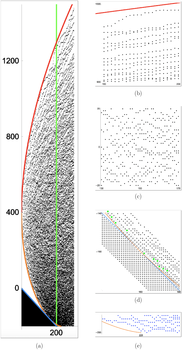
Figure 3: (a) A sample of the point process $\mathcal{L}(\vec{\lambda})=\{(j,\lambda^{(j)}_{i}-i):1\leq i\leq n,\,1\leq j\leq k\}$ obtained through the Berele insertion of $k$ random words with law (8.2) in the alphabet $\mathsf{A}_{n}$. Here we chose $n=200$, $k=300$. Red and orange curves denote respectively the upper and lower branch of the limit shape, computed in (8.10). The verical green line has abscissa $n$; the process to its left has the law of the oscillating symplectic Schur process (8.1).
(b) A close-up on the top edge of the liquid region.
(c) A close-up on the bulk of the liquid region.
(d) A close-up of the point process around the point $(4n/5,-4n/5)$. Green squares denote the first few levels of the complemented point configuration described in Section 8.5, which asymptotically converges to a GUE corners process.
(e) Blue points represent holes of the process $\mathcal{L}(\vec{\lambda})$. Portrayed is a close-up of the proximity of the point $(9n/8,-n)$, where the lower branch of the limit shape touches the horizontal line of ordinate $-n$.

8.1 Limit shape

Let us describe the macroscopic limit shape produced by the random point configuration $\mathcal{L}(\vec{\lambda})=\{(j,\lambda^{(j)}_{i}-i):1\leq i\leq n,\,1\leq j\leq k\}$, where $\vec{\lambda}=\{\lambda^{(i)}\}_{i=1,\dots,k}\subset\{1,\dots,k\}\times\mathbb{Z}$ is distributed according to the oscillating symplectic Schur process (8.1) after rescaling microscopic coordinates $(i,j)$ as $(nx,ny)$. First, we observe that $\lambda^{(i)}_{j}=0$ almost surely for all $n\geq j>i$, as a result of the Berele insertion mechanism. This implies that points $(i,-j)$ for $n\geq j>i$ belong almost surely to the configuration $\mathcal{L}(\vec{\lambda})$. Thus we refer to the set of macroscopic points $\{(x,y):x\in(0,1),\,y\in(-1,0),\,x+y\leq 0\}$ as the frozen region.

To describe the non-trivial part of the limit shape, we consider the correlation kernel obtained in 5.18. Up to a simple gauge transformation, the correlation kernel (5.16), with the choice of specializations prescribed by (8.1), describing the point configuration $\mathcal{L}(\vec{\lambda})$ equals

$$K^{\text{SSP}}(i,u;j,v)=\begin{dcases}\frac{1}{(2\pi\mathrm{i})^{2}}\oint_{\Gamma_{1-\delta}}\frac{\mathrm{d}z}{z}\oint_{\Gamma_{\frac{1}{2}+\delta}}\mathrm{d}w\,\frac{1-w^{2}}{(1-zw)(z-w)}\frac{G_{j,v}(z)}{G_{i,u}(w)},\qquad&\text{if }i\leq j,\\ \frac{1}{(2\pi\mathrm{i})^{2}}\oint_{\Gamma_{\frac{1}{2}+\delta}}\frac{\mathrm{d}z}{z}\oint_{\Gamma_{1-\delta}}\mathrm{d}w\,\frac{1-w^{2}}{(1-zw)(z-w)}\frac{G_{j,v}(z)}{G_{i,u}(w)},\qquad&\text{if }i>j.\end{dcases}$$ (8.3)

In this formula, we take any $\delta\in(0,1/4)$ and used the notations

$$\Gamma_{\rho} :=\{z\in\mathbb{C}\,:\,|z|=\rho\},$$

$$G_{j,v}(z) :=(1-z)^{-2n}[(1-z/2)(1-2z)]^{j}\,z^{-j-v}.$$

To understand limit shapes and limiting processes arising while scaling around various regions of the random field $\mathcal{L}(\vec{\lambda})$, we will perform an asymptotic analysis of the kernel $K^{\text{SSP}}$ by employing the saddle point method, as it has been done previously in the literature [OR-2003, OR-2006, OR-2007]. Under the scaling

$$j=nx,\qquad v=ny,$$

with $x\in(0,1),y\in\mathbb{R}$, and in the liquid region $x+y>0$, we observe that the function $G_{j,v}$ becomes

$$G_{j,v}(z)=\exp\left\{nh_{x,y}(z)\right\},$$

where the function $h_{x,y}$ in the exponent is

$$h_{x,y}(z)=-2\log(1-z)+x\log\left(1-\frac{z}{2}\right)+x\log\left(1-2z\right)-(x+y)\log(z).$$ (8.4)

The large $n$ behavior of $K^{\text{SSP}}$ is determined by the critical points of $h_{x,y}(z)$, i.e. by the roots of

$$h_{x,y}^{\prime}(z)=-\frac{x+y}{z}+\frac{2x}{2z-1}-\frac{x}{2-z}+\frac{2}{1-z},$$ (8.5)

or, collecting the terms,

$$h_{x,y}^{\prime}(z)=\frac{z^{3}(2x-2y-4)-z^{2}(2x-7y-10)-z(2x+7y+4)+2(x+y)}{(z-2)(z-1)z(2z-1)}.$$ (8.6)

Then $h_{x,y}^{\prime}(z)=0$ yields a cubic equation with coefficients parameterized by $x,y$. Studying the expression (8.5) we see that it always has a real zero, which we denote by $z_{0}$, in the half line $(2,+\infty)$; such zero will always be irrelevant for our asymptotic analysis. The two remaining zeros, which we denote by $z_{\pm}$, can have one of the following topologies, explained by Figure 4:

1. for $y\geq y_{+}(x)$, $z_{\pm}\in(1/2,1)$;

2. for $y_{-}(x)<y<y_{+}(x)$, $z_{\pm}$ are complex conjugate with non-zero imaginary part;

3. for $-x\leq y\leq y_{-}(x)$, $z_{\pm}\in(0,1/2)$;

4. for $y<-x$, $z_{-}<0$ and $z_{+}\in(0,1/2)$.

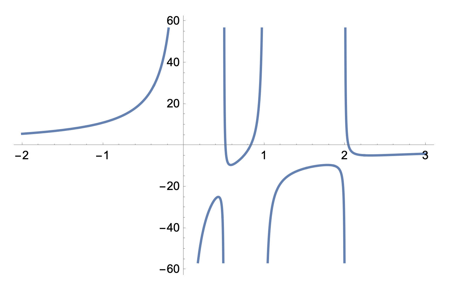
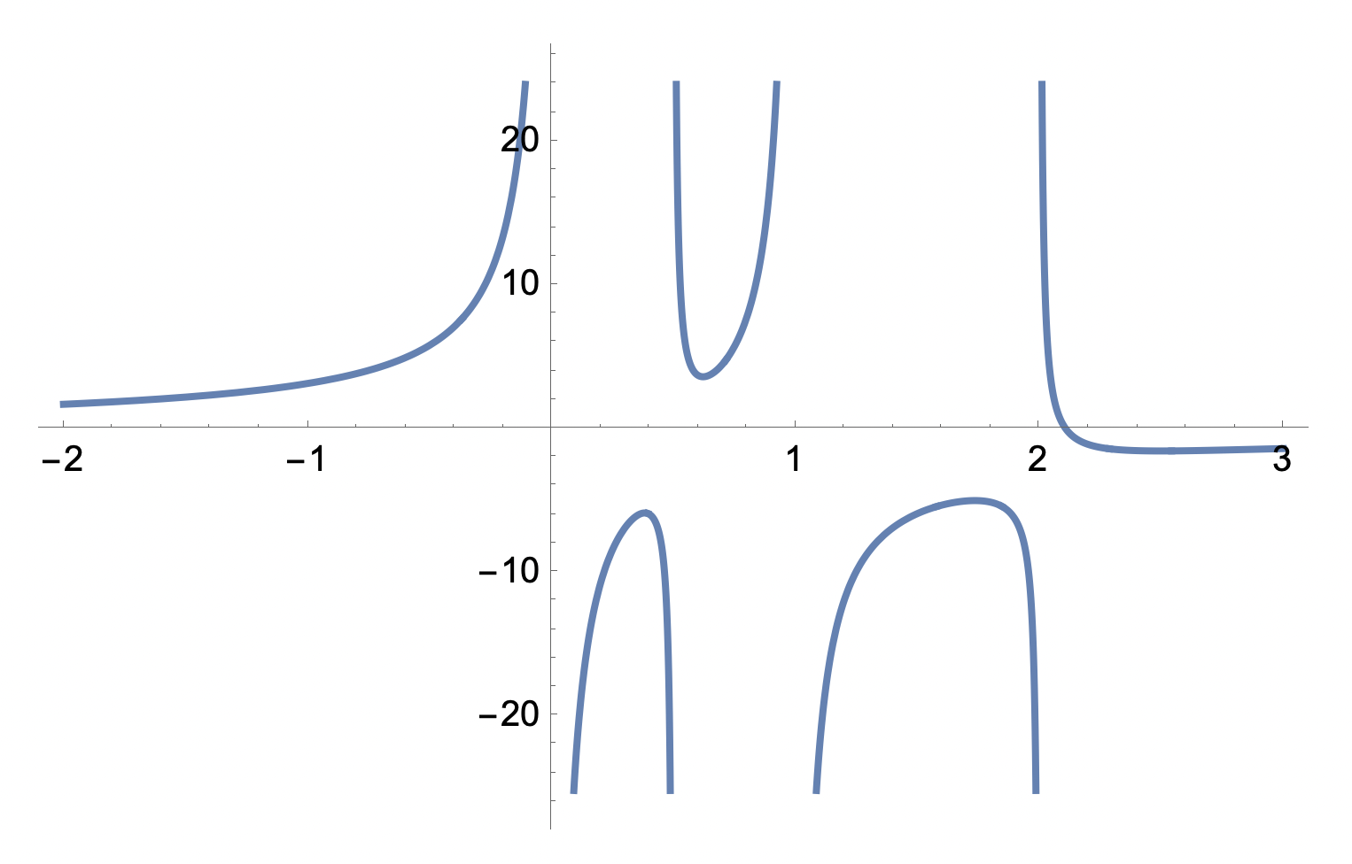
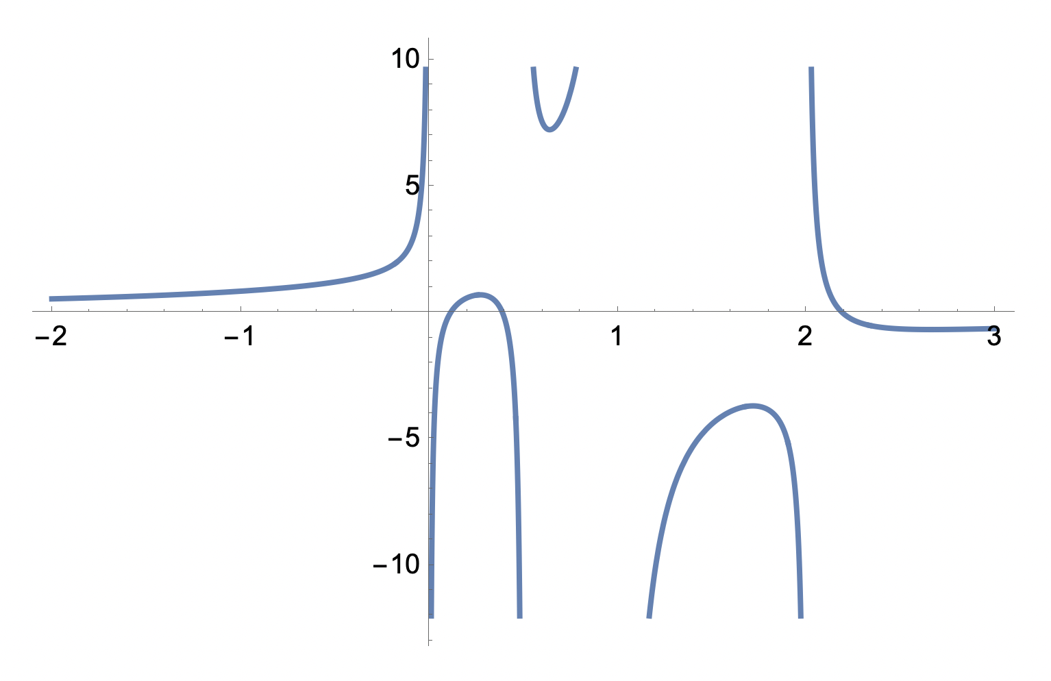
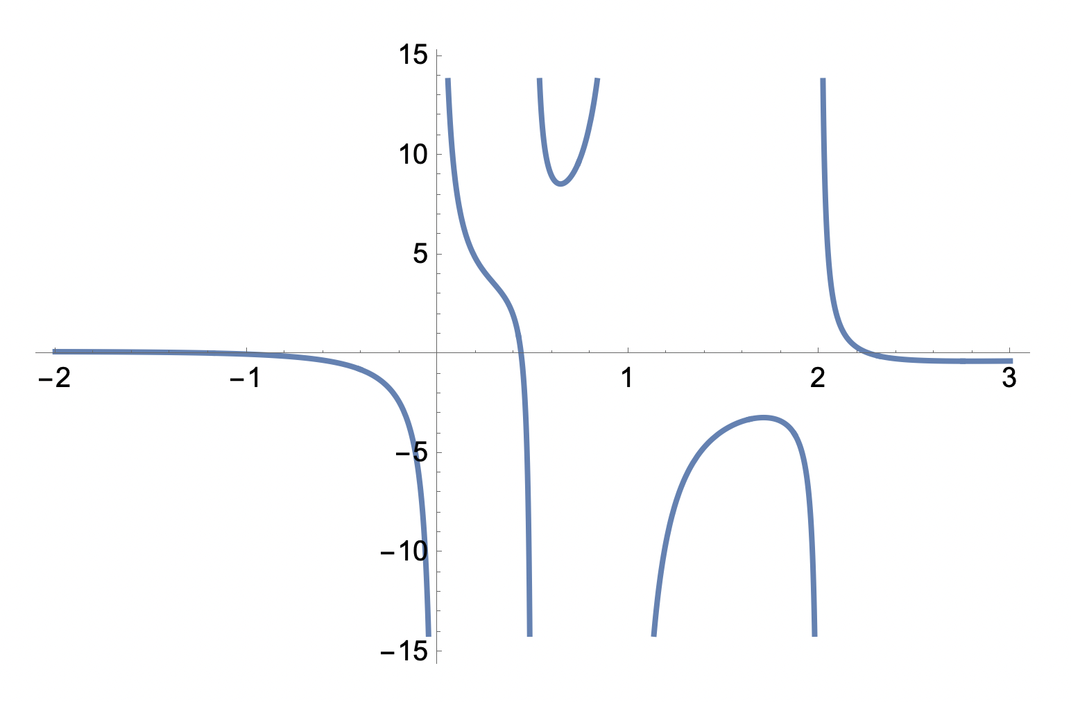
Figure 4: Plots of $h^{\prime}_{x,y}(z)$ for real $z$ and different values of $x,y$. From top-left to bottom-right these topologies correspond to the cases enumerated after Equation (8.6).

The functions $y_{\pm}(x)$ above are the unique real numbers such that there exists some $z_{0}\in\mathbb{R}$ with

$$h_{x,y(x)}^{\prime}(z_{0})=h_{x,y(x)}^{\prime\prime}(z_{0})=0.$$ (8.7)

We label $y_{+}(x)$ the larger and $y_{-}(x)$ the smaller of the two, so that $y_{+}(x)\geq y_{-}(x)$. Moreover, we label the corresponding $z_{0}$ in (8.7) by $z_{\mathrm{up}}(x)$ and $z_{\mathrm{down}}(x)$, respectively.

To find explicit expressions, let us solve directly the system the system of equations $h_{x,y}^{\prime}(z)=0$, $h_{x,y}^{\prime\prime}(z)=0$, which, after simple algebra and assuming $z\neq 0$, can be recast as the system:

$$\frac{1}{(1-z)^{2}}-\frac{x}{(z-2)^{2}}-\frac{x}{(1-2z)^{2}}=0,$$ (8.8)

$$y(x,z)=\frac{2z}{1-z}-\frac{xz}{2-z}+\frac{x}{2z-1}.$$ (8.9)

The two relevant solutions of (8.8) are given by

$$z_{\mathrm{up}}(x)=\frac{\sqrt{-18\sqrt{x^{3}(x+9)}-x(18x+11)+20\sqrt{x(x+9)}+36}}{10x-8}+\frac{9x-\sqrt{x(x+9)}-10}{10x-8},$$

$$z_{\mathrm{down}}(x)=\frac{9x+\sqrt{x(x+9)}-10}{10x-8}-\frac{\sqrt{18\sqrt{x^{3}(x+9)}-x(18x+11)-20\sqrt{x(x+9)}+36}}{10x-8},$$

so that plugging these expressions into (8.9), we obtain

$$y_{+}(x)=y(x,z_{\mathrm{up}}(x)),\qquad y_{-}(x)=y(x,z_{\mathrm{down}}(x)),$$ (8.10)

and their plots produce the red and orange curves portrayed in Figure 3. The lower branch of the limit shape $y_{-}$ is tangent to the line $y=-x$, which delimits the frozen region of fully packed particles. The tangency point is

$$x=4/5,\qquad y_{-}(4/5)=-4/5.$$

8.2 Limit process in the bulk: an extended Sine process

Fix $x\in(0,1)$ and $y\in(y_{-}(x),y_{+}(x))$. Let $z_{\pm}=z_{\pm}(x,y)$ be the complex conjugate roots of $h_{x,y}^{\prime}(z)=0$. Set $\gamma_{+}(z_{+})$ as a circle arc connecting $z_{-}$ to $z_{+}$ counterclockwise, crossing the segment $(1/2,2)$ and $\gamma_{-}(z_{+})$ as a circle arc connecting $z_{-}$ to $z_{+}$ clockwise, crossing $(-\infty,1/2)$. For the following result, define the kernel $\mathcal{K}_{\mathrm{bulk}}^{(z_{+})}:\mathbb{Z}^{2}\times\mathbb{Z}^{2}\to\mathbb{R}$ by

$$\mathcal{K}_{\mathrm{bulk}}^{(z_{+})}(\tau,\alpha;\tau^{\prime},\alpha^{\prime})=\begin{dcases}\frac{1}{2\pi\mathrm{i}}\int_{\gamma_{+}(z_{+})}(5/2-w-1/w)^{\tau^{\prime}-\tau}\,w^{\alpha-\alpha^{\prime}-1}\mathrm{d}w,\qquad&\text{if }\tau\leq\tau^{\prime},\\ \frac{1}{2\pi\mathrm{i}}\int_{\gamma_{-}(z_{+})}(5/2-w-1/w)^{\tau^{\prime}-\tau}\,w^{\alpha-\alpha^{\prime}-1}\mathrm{d}w,\qquad&\text{if }\tau>\tau^{\prime}.\end{dcases}$$

Proposition 8.1.

Consider the scaling

$$i(\tau)=\lfloor nx\rfloor+\tau,\qquad u(\alpha)=\lfloor ny\rfloor+\alpha.$$

Then, for any $k\in\mathbb{Z}_{\geq 1}$ and any pair of $k$-tuples $\tau_{1},\dots,\tau_{k},\alpha_{1},\dots,\alpha_{k}\in\mathbb{Z}$, denoting $i_{\ell}=i(\tau_{\ell})$, $u_{\ell}=u(\alpha_{\ell})$, we have

$$\lim_{n\to\infty}\,\det_{1\leq\ell,\ell^{\prime}\leq k}\left[K^{\text{SSP}}(i_{\ell},u_{\ell};i_{\ell^{\prime}},u_{\ell^{\prime}})\right]=\det_{1\leq\ell,\ell^{\prime}\leq k}\left[\mathcal{K}_{\mathrm{bulk}}^{(z_{+})}(\tau_{\ell},\alpha_{\ell};\tau_{\ell^{\prime}},\alpha_{\ell^{\prime}})\right].$$

The proof is analogous to [OR-2003] and therefore we do not provide details here.

8.3 Density in the bulk

The diagonal terms of our extended sine kernel $\mathcal{K}_{\mathrm{bulk}}^{(z_{+})}$ determine the density $\rho(x,y)$ of points in the process (8.1):

$$\rho(x,y)=\mathcal{K}_{\mathrm{bulk}}^{(z_{+})}(0,0;0,0)=\frac{\arg\left(z_{+}(x,y)\right)}{\pi}.$$ (8.11)

Using Cardano’s formula, we find $z_{+}(x,y)$ explicitly as the solution to the cubic equation (8.6) with $\Im(z_{+}(x,y))>0$; it is

$$z_{+}(x,y)=\frac{1}{6a(x,y)}\left(2b(x,y)-c(x,y)-\frac{\Delta_{0}(x,y)}{c(x,y)}+\mathrm{i}\sqrt{3}\left|c(x,y)-\frac{\Delta_{0}(x,y)}{c(x,y)}\right|\right),$$

where

$$a(x,y)=4-2x+2y,\qquad b(x,y)=10-2x+7y,$$

$$c(x,y)=\sqrt[3]{\frac{\Delta_{1}(x,y)+\sqrt{\Delta_{1}(x,y)^{2}-4\Delta_{0}(x,y)^{3}}}{2}},$$

and

$$\Delta_{0}(x,y)=16x^{2}+2xy-40x+7y^{2}+32y+52,$$

$$\Delta_{1}(x,y)=128x^{3}+24x^{2}y-264x^{2}+78xy^{2}-132xy-48x+20y^{3}+276y^{2}+816y+560.$$

Within the limit shape, $c(x,y)$ is a real number, assuming $\sqrt[3]{},\sqrt[2]{}$ to be the principal branches of the cube and square root. In fact, the limit shape, in the region $y\geq-1$, is characterized by the implicit equation

$$\Delta_{1}(x,y)^{2}-4\Delta_{0}(x,y)^{3}=0.$$

8.4 Edge asymptotics: Airy process

We can also comment on the nature of the scaled process around the limit shape. Following [OR-2007, Eqn. (60)], recall that the extended Airy kernel $K_{\mathrm{Airy}}:\mathbb{R}^{2}\times\mathbb{R}^{2}\to\mathbb{R}$ is:

$$\begin{split}K_{\mathrm{Airy}}(\tau,\alpha;\tau^{\prime},\alpha^{\prime}):=&-\mathbf{1}_{\tau>\tau^{\prime}}\,\frac{e^{-\frac{(\alpha-\alpha^{\prime})^{2}}{2(\tau-\tau^{\prime})}}}{\sqrt{2\pi(\tau-\tau^{\prime})}}\\ &\qquad+\int_{e^{-\mathrm{i}\pi/3}\infty}^{e^{\mathrm{i}\pi/3}\infty}\frac{\mathrm{d}\xi}{2\pi\mathrm{i}}\int_{e^{-\mathrm{i}2\pi/3}\infty}^{e^{\mathrm{i}2\pi/3}\infty}\frac{\mathrm{d}\eta}{2\pi\mathrm{i}}\,\frac{1}{\xi-\eta}\,e^{\frac{\xi^{3}-\eta^{3}}{3}-\frac{\xi^{2}\tau^{\prime}-\eta^{2}\tau}{2}-\xi\alpha^{\prime}+\eta\alpha}.\end{split}$$

Alternatively, this kernel can be written in terms of Airy functions, hence the name; see [FNH-1999, Mac-1994, PS-2002, Joh-2003].

Proposition 8.2.

Fix $x\in(0,1)$ and let $(y,z_{*})$ be either $(y_{-}(x),z_{\mathrm{down}}(x))$ or $(y_{+}(x),z_{\mathrm{up}}(x))$. Define parameters

$$d_{1}:=\left(\frac{h_{x,y}^{\prime\prime\prime}(z_{*})}{2}\right)^{\!\!\frac{1}{3}}z_{*},\qquad c_{1}:=\frac{(2z_{*}-1)^{2}(z_{*}-2)^{2}}{2z_{*}\left(5z_{*}^{2}-8z_{*}+5\right)}\,d_{1}^{2},\qquad c_{2}:=\frac{2(z_{*}^{2}-1)}{(z_{*}-2)(2z_{*}-1)}\,c_{1},$$

and consider the scaling

$$i(\tau)=\left\lfloor xn+c_{1}\tau n^{\frac{2}{3}}\right\rfloor,\qquad u(\tau,\alpha)=\left\lfloor yn+c_{2}\tau n^{\frac{2}{3}}+d_{1}\alpha n^{\frac{1}{3}}\right\rfloor.$$

Then, for any $k\in\mathbb{Z}_{\geq 1}$ and any pair of $k$-tuples $\tau_{1},\dots,\tau_{k},\alpha_{1},\dots,\alpha_{k}\in\mathbb{R}$, denoting $i_{\ell}=i(\tau_{\ell})$, $u_{\ell}=u(\tau_{\ell},\alpha_{\ell})$, we have:

• if $y=y_{+}(x)$ and $x\in(0,1)$ or $y=y_{-}(x)$ and $x\in(0,\frac{4}{5})$, then

  $$\lim_{n\to\infty}\,\det_{1\leq\ell,\ell^{\prime}\leq k}\left[n^{\frac{1}{3}}|d_{1}|\,K^{\text{SSP}}(i_{\ell},u_{\ell};i_{\ell^{\prime}},u_{\ell^{\prime}})\right]=\det_{1\leq\ell,\ell^{\prime}\leq k}\left[K_{\mathrm{Airy}}(\tau_{\ell},\alpha_{\ell};\tau_{\ell^{\prime}},\alpha_{\ell^{\prime}})\right];$$ (8.12)

• if $y=y_{-}(x)$ and $x\in(\frac{4}{5},1)$, then

  $$\lim_{n\to\infty}\,\det_{1\leq\ell,\ell^{\prime}\leq k}\left[n^{\frac{1}{3}}|d_{1}|\!\left(\delta_{i_{\ell},i_{\ell^{\prime}}}\delta_{u_{\ell},u_{\ell^{\prime}}}-K^{\text{SSP}}(i_{\ell},u_{\ell};i_{\ell^{\prime}},u_{\ell^{\prime}})\right)\right]=\det_{1\leq\ell,\ell^{\prime}\leq k}\left[K_{\mathrm{Airy}}(\tau_{\ell},\alpha_{\ell};\tau_{\ell^{\prime}},\alpha_{\ell^{\prime}})\right].$$ (8.13)

The proof is analogous to [OR-2003], therefore we do not provide details here.

Remark 8.3.

If $x\in(0,1)$ and $(y,z_{*})=(y_{+}(x),z_{\textrm{up}}(x))$, then $z_{*}\in(\frac{1}{2},1)$, $h_{x,y}^{\prime\prime\prime}(z_{*})>0$, implying that $d_{1},c_{1},c_{2}>0$. If $x\in(0,\frac{4}{5})$ and $(y,z_{*})=(y_{-}(x),z_{\textrm{down}}(x))$, then $z_{*}\in(0,\frac{1}{2})$, $h_{x,y}^{\prime\prime\prime}(z_{*})<0$, implying $c_{1}>0>d_{1},c_{2}$. Finally, if $x\in(\frac{4}{5},1)$ and $(y,z_{*})=(y_{-}(x),z_{\textrm{down}}(x))$, then $z_{*}\in(-\frac{1}{2},0)$, $h_{x,y}^{\prime\prime\prime}(z_{*})>0$, implying $c_{2}>0>d_{1},c_{1}$.

Remark 8.4.

The left hand side of (8.12) differs from that of (8.13) since in the latter, the extended Airy process arises from considering the “holes” of the point process rather than the points themselves.

Remark 8.5.

The kernel $K^{\text{SSP}}$ in (8.3) differs from that of the ordinary Schur process [Ok-2001b] by the presence of the cross factor $(1-w^{2})/(1-wz)(z-w)$, which replaces $1/(z-w)$. From the standpoint of saddle point asymptotic analysis, such factor transforms, after scaling integration variables $z=z_{*}+\varepsilon\xi$ and $w=z_{*}+\varepsilon\eta$ around a saddle point $z_{*}$, as

$$\frac{(1-w^{2})}{(1-wz)(z-w)}=\frac{1}{\varepsilon}\cdot\frac{1}{\xi-\eta}+O(1),\,\text{ as }\epsilon\to 0^{+},$$

whenever $z_{*}\neq\pm 1$. Therefore, for saddle points $z_{*}\neq\pm 1$, the asymptotic behaviour of $K^{\text{SSP}}$, and hence of the symplectic Schur process, is equivalent to the ordinary Schur process.

Remark 8.6.

The argument of 8.5 holds whenever the dominant saddle point $z_{*}$ of the function $h_{x,y}(z)$ is different than $\pm 1$. From (8.5), we see that $h_{x,y}^{\prime}(z)$ always has a singularity at $z=1$ (and so $z=1$ is never a saddle point), while

$$h_{x,y}^{\prime}(-1)=1+y.$$

Therefore $h_{x,y}$ has a singularity at $z=-1$ for $y=-1$ and evaluating higher order derivatives we see

$$h_{x,-1}^{\prime\prime}(-1)=-\frac{1}{2}+\frac{4}{9}x,\qquad h_{x,-1}^{\prime\prime\prime}(-1)=-\frac{3}{2}+\frac{4}{3}x.\qquad h_{x,-1}^{\prime\prime\prime\prime}(-1)=-\frac{21}{4}+\frac{128}{27}x,$$ (8.14)

which implies that second order singularities at $z=-1$ can only take place setting $x=9/8,y=-1$, which falls outside of the probabilistic region ($0<x\leq 1$) for the symplectic Schur process. Interestingly, at $(x,y)=(9/8,-1)$, the point $z=-1$ is a singularity of fourth order, as can be seen from (8.14). The asymptotic limit of the kernel $K^{\text{SSP}}$ is not the extended Airy kernel in this case, but instead a Pearcey-like kernel that will be reported in Section 8.6.

8.5 Tangency points asymptotics: GUE corners process

We analyze the point process in the neighborhood of the tangency points of the limit shape with the frozen regions. Following [OR-2006, Eqn. (14)], see also [Joh-2005, JN-2006], define the kernel $\mathcal{K}_{\mathrm{GUEcor}}:\left(\mathbb{Z}_{>0}\times\mathbb{R}\right)\times\left(\mathbb{Z}_{>0}\times\mathbb{R}\right)\to\mathbb{R}$ by

$$\begin{split}\mathcal{K}_{\mathrm{GUEcor}}(i,\alpha;j,\alpha^{\prime})=&-\mathbf{1}_{i>j}\mathbf{1}_{\alpha>\alpha^{\prime}}\,\frac{(\alpha-\alpha^{\prime})^{i-j-1}}{(i-j-1)!}\\ &\qquad+\int_{\mathrm{i}\mathbb{R}+1}\frac{\mathrm{d}\xi}{2\pi\mathrm{i}}\oint_{\Gamma_{\frac{1}{2}}}\frac{\mathrm{d}\eta}{2\pi\mathrm{i}}\,\frac{1}{\xi-\eta}\frac{\xi^{j}}{\eta^{i}}\,e^{\frac{\xi^{2}-\eta^{2}}{2}-\alpha^{\prime}\xi+\alpha\eta}.\end{split}$$

The point process having correlation kernel $\mathcal{K}_{\mathrm{GUEcor}}$ is the GUE corners process, which describes the eigenvalues of corners of an infinite Gaussian Hermitian random matrix, as in [OV-1996]. Equivalently, this means that the projection of the kernel $\mathcal{K}_{\mathrm{GUEcor}}$ to $\{1,\dots,N\}\times\mathbb{R}$ describes the eigenvalues of principal minors of an $N\times N$ GUE random matrix.

Proposition 8.7 (GUE corners process at the tangency point $(0,2)$).

Consider the scaling

$$u(\alpha)=2n+\lfloor 2\alpha\sqrt{n}\rfloor.$$

For any $k\in\mathbb{Z}_{\geq 1}$ and any pair of $k$-tuples $i_{1},\dots,i_{k}\in\mathbb{Z}_{>0}$, and pairwise distinct $\alpha_{1},\dots,\alpha_{k}\in\mathbb{R}$, let us denote $u_{\ell}=u(\alpha_{\ell})$, then:

$$\lim_{n\to\infty}\,\det_{1\leq\ell,\ell^{\prime}\leq k}\left[2\sqrt{n}\,K^{\text{SSP}}(i_{\ell},u_{\ell};i_{\ell^{\prime}},u_{\ell^{\prime}})\right]=\det_{1\leq\ell,\ell^{\prime}\leq k}\left[\mathcal{K}_{\mathrm{GUEcor}}(i_{\ell},\alpha_{\ell};i_{\ell^{\prime}},\alpha_{\ell^{\prime}})\right].$$

The GUE corners process can also be observed at the tangency point $(x,y)=(4/5,-4/5)$ after a certain complementation of the point configuration, which we briefly explain next. The point process $\mathcal{L}(\vec{\lambda})$, around the microscopic location $(4n/5,-4n/5)$, tends to occupy diagonal segments of the form $(i,j),\dots,(i+k,j-k)$ with length $k=O(\sqrt{n})$. The complemented process that should be considered for asymptotics, depicted in Figure 3(d), consists of points $(i+1,j-1)$ if $(i,j)$ is occupied, but $(i+1,j-1)$ is not (this happens when $(i,j)$ is the down-right endpoint of a filled diagonal segment) and points $(i,j+1)$ if $(i,j)$ is occupied, but $(i-1,j+1)$ is not (here $(i,j)$ is the up-left endpoint of a filled diagonal segment). This complementation procedure consists, in the language of lozenge tilings (which are in correspondence with interlacing partitions), in considering different types of lozenges in the neighborhood of the tangency point; see e.g. [Gor-2021]. Finally, we point out that the point configuration $\mathcal{L}(\vec{\lambda})$ originating from the symplectic Schur process does not consist of interlacing partitions, nevertheless asymptotically, around the tangency point, this identification can be made.

8.6 Bottom edge asymptotics at $x=9/8$.

In the previous subsections, we provided arguments to show that, for any $x\in(0,1)$, the symplectic Schur process converges asymptotically to a multilivel extension of the Sine process in the bulk and of the Airy process at the edge. We also gave explicit formulas for the limit shape. In this subsection, we do the asymptotic analysis in a neighborhood of the macroscopic point $(x,y)=(9/8,-1)$. This would correspond formally to the region where the bottom branch of the limit shape touches the horizontal line $y=-1$; see Figure 3 (e). We say formally because, as we have explained before, the symplectic Schur process does not describe the limit shape for $x>1$.

To state our result, we introduce the kernel $\mathcal{K}:(\mathbb{R}\times\mathbb{R}_{>0})\times(\mathbb{R}\times\mathbb{R}_{>0})\to\mathbb{R}$ given by

$$\begin{split}\mathcal{K}(\tau,\alpha;\tau^{\prime},\alpha^{\prime}):=&\,\mathbf{1}_{\tau<\tau^{\prime}}\,\frac{e^{-\frac{(\alpha^{\prime}-\alpha)^{2}}{2(\tau^{\prime}-\tau)}}}{\sqrt{2\pi(\tau^{\prime}-\tau)}}\\ &\qquad+\int_{e^{-3\mathrm{i}\pi/4}\infty}^{e^{3\mathrm{i}\pi/4}\infty}\frac{\mathrm{d}\xi}{2\pi\mathrm{i}}\int_{-\mathrm{i}\infty}^{+\mathrm{i}\infty}\frac{\mathrm{d}\eta}{2\pi\mathrm{i}}\,\frac{2\eta}{\eta^{2}-\xi^{2}}\,e^{\frac{\xi^{4}-\eta^{4}}{24}+\frac{\tau^{\prime}\xi^{2}-\tau\eta^{2}}{2}-\alpha^{\prime}\xi+\alpha\eta},\end{split}$$ (8.15)

where the $\xi$-contour lies in the complex half-plane $\Re(\xi)\leq 0$.

Proposition 8.8.

Consider the scaling

$$i(\tau)=\left\lfloor\frac{9n}{8}+\sqrt{\frac{27n}{64}}\,\tau\right\rfloor,\qquad u(\alpha)=-n+\left\lfloor\left(\frac{n}{12}\right)^{\!\frac{1}{4}}\alpha\right\rfloor.$$ (8.16)

Then, for any $k\in\mathbb{Z}_{\geq 1}$ and any pair of $k$-tuples $\tau_{1},\dots,\tau_{k}\in\mathbb{R}$, $\alpha_{1},\dots,\alpha_{k}\in\mathbb{R}_{+}$, denoting $i_{\ell}=i(\tau_{\ell})$, $u_{\ell}=u(\alpha_{\ell})$, we have:

$$\lim_{n\to\infty}\,\det_{1\leq\ell,\ell^{\prime}\leq k}\left[\left(\frac{n}{12}\right)^{\!\frac{1}{4}}\left(\delta_{i_{\ell},i_{\ell^{\prime}}}\delta_{u_{\ell},u_{\ell^{\prime}}}-K^{\text{SSP}}(i_{\ell},u_{\ell};i_{\ell^{\prime}},u_{\ell^{\prime}})\right)\right]=\det_{1\leq\ell,\ell^{\prime}\leq k}\left[\mathcal{K}(\tau_{\ell},\alpha_{\ell};\tau_{\ell^{\prime}},\alpha_{\ell^{\prime}})\right].$$ (8.17)

Since the limit (8.17) appears to be new, we report its proof, although the proof just amounts to an application of the saddle point method as in the previous subsections.

Proof.

Under the scaling (8.16), we write the kernel (8.3), after shifting contours and evaluating the $z$-pole at $z=w$, as

$$K^{\text{SSP}}(i(\tau),u(\alpha);\,i(\tau^{\prime}),u(\alpha^{\prime}))=\ \delta_{\tau,\tau^{\prime}}\,\delta_{\alpha,\alpha^{\prime}}+\mathbf{1}_{\tau<\tau^{\prime}}\,\frac{1}{2\pi\mathrm{i}}\oint_{\Gamma_{1-\delta}}\frac{\mathrm{d}w}{w}\,\frac{G_{i(\tau^{\prime}),u(\alpha^{\prime})}(w)}{G_{i(\tau),u(\alpha)}(w)}\\ +\frac{1}{(2\pi\mathrm{i})^{2}}\oint_{\Gamma_{\frac{1}{2}+\delta}}\frac{\mathrm{d}z}{z}\oint_{\Gamma_{1-\delta}}\mathrm{d}w\,\frac{1-w^{2}}{(1-wz)(z-w)}\frac{G_{i(\tau^{\prime}),u(\alpha^{\prime})}(z)}{G_{i(\tau),u(\alpha)}(w)}.$$ (8.18)

Computations from 8.6 show that the function $h_{x,y}$ from (8.4) has a critical point of fourth order at $x=9/8,y=-1,z=-1$:

$$h_{\frac{9}{8},-1}^{\prime}(-1)=h_{\frac{9}{8},-1}^{\prime\prime}(-1)=h_{\frac{9}{8},-1}^{\prime\prime\prime}(-1)=0,\qquad h_{\frac{9}{8},-1}^{\prime\prime\prime\prime}(-1)=\frac{1}{12}.$$

Considering the scaling (8.16) and

$$z=-1+\left(\frac{n}{12}\right)^{\!-\frac{1}{4}}\xi,\qquad w=-1+\left(\frac{n}{12}\right)^{\!-\frac{1}{4}}\eta,$$

we have

$$G_{i(\tau^{\prime}),u(\alpha^{\prime})}(z)=\exp\left\{nh_{\frac{1}{n}i(\tau^{\prime}),\frac{1}{n}u(\alpha^{\prime})}(z)\right\}\approx c_{n}(\tau^{\prime},\alpha^{\prime})\exp\left\{\frac{\xi^{4}}{24}+\frac{\tau^{\prime}\xi^{2}}{2}+\alpha^{\prime}\xi\right\},$$

where the term $c_{n}(\tau^{\prime},\alpha^{\prime})$ above does not depend on $\xi$. A similar estimate holds for $G_{i(\tau),u(\alpha)}(w)$, except that $\xi,\tau^{\prime},\alpha^{\prime}$ must be replaced by $\eta,\tau,\alpha$, respectively. It follows that

$$\frac{G_{i(\tau^{\prime}),u(\alpha^{\prime})}(w)}{G_{i(\tau),u(\alpha)}(w)} \approx\frac{c_{n}(\tau^{\prime},\alpha^{\prime})}{c_{n}(\tau,\alpha)}\,e^{\frac{(\tau^{\prime}-\tau)\eta^{2}}{2}+(\alpha^{\prime}-\alpha)\eta},$$

$$\frac{G_{i(\tau^{\prime}),u(\alpha^{\prime})}(z)}{G_{i(\tau),u(\alpha)}(w)} \approx\frac{c_{n}(\tau^{\prime},\alpha^{\prime})}{c_{n}(\tau,\alpha)}\,e^{\frac{\xi^{4}-\eta^{4}}{24}+\frac{\tau^{\prime}\xi^{2}-\tau\eta^{2}}{2}+\alpha^{\prime}\xi-\alpha\eta}.$$

Moreover,

$$\frac{\mathrm{d}z}{z}\approx-\left(\frac{n}{12}\right)^{\!-\frac{1}{4}}\mathrm{d}\xi,\qquad\mathrm{d}w\approx\left(\frac{n}{12}\right)^{\!-\frac{1}{4}}\mathrm{d}\eta,\qquad\frac{1-w^{2}}{(1-wz)(z-w)}\approx\left(\frac{n}{12}\right)^{\!\frac{1}{4}}\frac{2\eta}{\xi^{2}-\eta^{2}}.$$

To obtain the final answer, first deform the $z$-contour to be of steepest descent and the $w$-contour to be of steepest ascent (as shown in Figure 5), then plug all estimates above into the formula (8.18) for the kernel $K^{\text{SSP}}$, next remove the gauge factor $c_{n}(\tau^{\prime},\alpha^{\prime})/c_{n}(\tau,\alpha)$, as it disappears when one considers determinants as in (8.17), then compute the Gaussian integral resulting from the first line in (8.18), and finally make a change of variables $\xi\mapsto-\xi$, $\eta\mapsto-\eta$ in the integral resulting from the second line in (8.18).

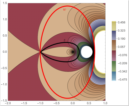
Figure 5: The contourplot of $\zeta\to\Re\left\{h_{\frac{9}{8},-1}(\zeta)\right\}-h_{\frac{9}{8},-1}(-1)$. Overlayed black and red curves are $z$ and $w$ integration curves deformed to be respectively of steepest descent and steepest ascent for $\Re\left\{h_{\frac{9}{8},-1}(\zeta)\right\}$.

∎

Remark 8.9.

The kernel $\mathcal{K}$ in (8.15) resembles the Pearcey kernel from [OR-2007, Eqn. (72)], see also [BH-1998a, BH-1998b, TW-2006], which has the form

$$\begin{split}\mathcal{K}(\tau,\alpha;\tau^{\prime},\alpha^{\prime}):=\,&\mathbf{1}_{\tau<\tau^{\prime}}\,\frac{e^{-\frac{(\alpha^{\prime}-\alpha)^{2}}{2(\tau^{\prime}-\tau)}}}{\sqrt{2\pi(\tau^{\prime}-\tau)}}\\ &\qquad+\left(\int_{e^{\mathrm{i}\pi/4}\infty}^{e^{-\mathrm{i}\pi/4}\infty}+\int_{e^{-\mathrm{i}3\pi/4}\infty}^{e^{\mathrm{i}3\pi/4}\infty}\right)\frac{\mathrm{d}\xi}{2\pi\mathrm{i}}\int_{-\mathrm{i}\infty}^{+\mathrm{i}\infty}\frac{\mathrm{d}\eta}{2\pi\mathrm{i}}\,\frac{1}{\xi-\eta}\,e^{\frac{\xi^{4}-\eta^{4}}{24}+\frac{\tau^{\prime}\xi^{2}-\tau\eta^{2}}{2}-\alpha^{\prime}\xi+\alpha\eta}.\end{split}$$

The differences are the integration contours for the $\xi$ variable and the cross terms, the one of our kernel being $\frac{2\eta}{\eta^{2}-\xi^{2}}$. One can draw a parallel with the case of the Airy kernel, where the presence of a similar cross term transforms the $\mathrm{Airy}_{2}$ kernel into the $\mathrm{Airy}_{2\to 1}$ kernel.

Remark 8.10.

In [BK-2010], a variant of the Pearcey kernel, dubbed the symmetric Pearcey kernel, was introduced to describe point processes produced by non-intersecting random walks conditioned to not cross a wall [KMFW-2011, Kuan-2013]. Despite the similarity with the process performed by the last row of the partitions $\lambda^{(j)}$ from our Berele insertion process, the kernels from [BK-2010] and (8.15) appear to be different. We hope to offer clarifications concerning relations between these processes and correlation kernels in future works.

An interesting observation is that the limit shape in the (not probabilistic) case of $x=9/8$, possesses a cubic singularity near the point $y=-1$ and this can be confirmed by using (8.11). First, write

$$h_{\frac{9}{8},-1+\varepsilon}^{\prime}(z)=\frac{(z+1)^{3}}{4(z-2)(z-1)z(2z-1)}-\frac{\varepsilon}{z}.$$

Then, for $\varepsilon>0$ small, we can express the root $z_{+}$ of $h^{\prime}_{\frac{9}{8},-1+\varepsilon}(z)$ as

$$z_{+}=-1+(3^{2/3}+3^{7/6}\mathrm{i})\varepsilon^{1/3}+o(\varepsilon^{1/3}),$$

which implies that

$$\frac{\arg(z_{+})}{\pi}=1-\frac{3^{7/6}}{\pi}\varepsilon^{1/3}+o(\varepsilon^{1/3}).$$

Cubic cusps of equilibrium measures, or limit shapes, are known to be related to the Pearcey process [BH-1998a, BH-1998b]. This observation offers a further invitation to a more rigorous study of the process $\mathcal{L}(\vec{\lambda})$ around the macroscopic region $(x,y)=(9/8,-1)$, which we hope to cover in future works.

Cesar Cuenca:

Department of Mathematics, The Ohio State University, Columbus, OH, USA.

Email address: cesar.a.cuenk@gmail.com

Matteo Mucciconi:

Department of Statistics, University of Warwick, Coventry, UK.

Email address: matteomucciconi@gmail.com

References

- [AB-2024] Amol Aggarwal and Alexei Borodin. Colored Line Ensembles for Stochastic Vertex Models. Preprint; arXiv:2402.06868 (2024).
- [ASW-1952] Michael Aissen, Isaac Jacob Schoenberg and Anne M. Whitney. On the generating functions of totally positive sequences I. Journal d’Analyse Mathématique 2, no. 1 (1952), pp. 93–103.
- [AFHSA-2023] Seamus P. Albion, Ilse Fischer, Hans Hongesberg and Florian Schreier-Aigner. Skew Symplectic and Orthogonal Characters Through Lattice Paths. Preprint; arXiv:2305.11730 (2023).
- [Ber-1986] Allan Berele. A Schensted-type correspondence for the symplectic group. Journal of Combinatorial Theory, Series A 43, no. 2 (1986), pp. 320–328.
- [Bet-2018] Dan Betea. Correlations for symplectic and orthogonal Schur measures. Preprint; arXiv:1804.08495 (2018).
- [Bet-2020] Dan Betea. Determinantal point processes from symplectic and orthogonal characters and applications. Séminaire Lotharingien de Combinatoire B 84 (2020).
- [BNNSS-2024+] Dan Betea, Anton Nazarov, Pavel Nikitin, Daniil Sarafnnikov and Travis Scrimshaw. Limit shapes from skew -duality and free fermions. In preparation.
- [Bor-2007] Alexei Borodin. Periodic Schur process and cylindric partitions. Duke Mathematical Journal 140, no. 3 (2007) pp. 391–468.
- [Bor-2011] Alexei Borodin. Schur dynamics of the Schur processes. Advances in Mathematics 228, no. 4 (2011), pp. 2268–2291.
- [BC-2014] Alexei Borodin and Ivan Corwin. Macdonald processes. Probability Theory and Related Fields, Volume 158 (2014), pp. 225–400.
- [BF-2014] Alexei Borodin and Patrik Ferrari. Anisotropic growth of random surfaces in 2+1 dimensions. Communications in Mathematical Physics 325, no. 2 (2014), pp. 603–684.
- [BG-2009] Alexei Borodin and Vadim Gorin. Shuffling algorithm for boxed plane partitions. Advances in Mathematics 220, no. 6 (2009), pp. 1739–1770.
- [BG-2015] Alexei Borodin and Vadim Gorin. General -Jacobi Corners Process and the Gaussian Free Field. Communications on Pure and Applied Mathematics 68, no. 10 (2015), pp. 1774–1844.
- [BG-2016] Alexei Borodin and Vadim Gorin. Lectures on integrable probability. Probability and Statistical Physics in St. Petersburg 91 (2016), pp. 155–214.
- [BK-2010] Alexei Borodin and Jeffrey Kuan. Random surface growth with a wall and Plancherel measures for . Communications in Pure and Applied Mathematics 63 (2010), pp. 831–894.
- [BO-2005] Alexei Borodin and Grigori Olshanski. Random partitions and the gamma kernel. Advances in Mathematics 194, no. 1 (2005), pp. 141–202.
- [BO-2017] Alexei Borodin and Grigori Olshanski. Representations of the infinite symmetric group. Vol. 160. Cambridge University Press, 2017.
- [BP-2014] Alexei Borodin and Leonid Petrov. Integrable probability: From representation theory to Macdonald processes. Probability Surveys 11 (2014), pp. 1–58.
- [BP-2016] Alexei Borodin and Leonid Petrov. Nearest neighbor Markov dynamics on Macdonald processes. Advances in Mathematics 300 (2016), pp. 71–155.
- [BR-2005] Alexei Borodin and Eric M. Rains. Eynard-Mehta theorem, Schur process, and their Pfaffian analogs. Journal of Statistical Physics 121 (2005), pp. 291–317.
- [BH-1998a] Edouard Brezin and Shinobu Hikami. Universal singularity at the closure of a gap in a random matrix theory. Physical Review E: Statistical, Nonlinear, and Soft Matter Physics 57, no. 4 (1998), pp. 4140–4149.
- [BH-1998b] Edouard Brezin and Shinobu Hikami. Level spacing of random matrices in an external source. Physical Review E: Statistical, Nonlinear, and Soft Matter Physics 58, no. 6 (1998), pp. 7176–7185.
- [BP-2019] Alexey Bufetov and Leonid Petrov. Yang-Baxter field for Spin Hall-Littlewood Symmetric Functions. Forum of Mathematics, Sigma; 7:e39 (2019).
- [BMP-2021] Alexey Bufetov, Matteo Mucciconi and Leonid Petrov. Yang-Baxter random fields and stochastic vertex models. Advances in Mathematics, Volume 388 (2021), 107865.
- [CGK-2022] Sylvie Corteel, Andrew Gitlin and David Keating. Colored vertex models and k-tilings of the Aztec diamond. Preprint; arXiv:2202.06020 (2022).
- [CH-2014] Ivan Corwin and Alan Hammond. Brownian Gibbs property for Airy line ensembles. Inventiones Mathematicae 195 (2014), pp. 441–508.
- [Cue-2018a] Cesar Cuenca. BC Type Z-measures and Determinantal Point Processes. Advances in Mathematics 334 (2018), pp. 1–80.
- [Cue-2018b] Cesar Cuenca. Markov processes on the duals to infinite-dimensional Lie groups, Annales de l’Institut Henri Poincaré: Probabilités et Statistiques, vol. 54, no. 3 (2018), pp. 1359–1407.
- [CG-2020] Cesar Cuenca and Vadim Gorin. -Deformed character theory for infinite-dimensional symplectic and orthogonal groups. Selecta Mathematica 26 (2020), pp. 1–55.
- [DF-1990] Percy Diaconis and James A. Fill. Strong stationary times via a new form of duality. Annals of Probability 18, no. 4 (1990), pp. 1483–1522.
- [Edr-1952] Albert Edrei. On the generating functions of totally positive sequences II. Journal d’Analyse Mathématique 2, no. 1 (1952), pp. 104–109.
- [EM-1998] Bertrand Eynard and Madan Lal Mehta. Matrices coupled in a chain: I. Eigenvalue correlations. Journal of Physics A: Mathematical and General 31, no. 19 (1998), pp. 4449–4456.
- [FNH-1999] Peter J. Forrester, Taro Nagao and Graeme Honner. Correlations for the orthogonal-unitary and symplectic-unitary transitions at the hard and soft edges. Nuclear Physics B 553, no. 3 (1999), pp. 601–643.
- [GOY-2021] Shiliang Gao, Gidon Orelowitz and Alexander Yong. Newell-Littlewood numbers. Transactions of the American Mathematical Society 374, no. 9 (2021), pp. 6331–6366.
- [GP-2024] Svetlana Gavrilova and Leonid Petrov. Tilted biorthogonal ensembles. Grothendieck random partitions, and determinantal tests. Selecta Mathematica 30, no. 56 (2024).
- [Gor-2021] Vadim Gorin. Lectures on Random Lozenge Tilings. Cambridge University Press; 2021.
- [HK-2022] Taehyeok Heo and Jae-Hoon Kwon. Combinatorial Howe duality of symplectic type. Journal of Algebra, vol. 600 (2022), pp. 1–44.
- [Howe-1989] Roger Howe. Remarks on classical invariant theory. Transactions of the American Mathematical Society 313, no. 2 (1989), pp. 539–570.
- [IMS-2023] Takashi Imamura, Matteo Mucciconi and Tomohiro Sasamoto. Skew RSK dynamics: Greene invariants, affine crystals and applications to -Whittaker polynomials. Forum of Mathematics, Pi; 11:e27 (2023).
- [JLW-2024] Naihuan Jing, Zhijun Li and Danxia Wang. Skew Symplectic and Orthogonal Schur Functions. SIGMA 20 (2024), 041.
- [Joh-2003] Kurt Johansson. Discrete Polynuclear Growth and Determinantal Processes. Communications in Mathematical Physics 242 (2003), pp. 277–329.
- [Joh-2005] Kurt Johansson. The Arctic Circle Boundary and the Airy Process. The Annals of Probability, vol. 33, no. 1 (2005), pp. 1–30.
- [JN-2006] Kurt Johansson and Eric Nordenstam. Eigenvalues of GUE Minors. Electronic Journal of Probability 11 (2006), pp. 1342–1371.
- [KN-1994] Masaki Kashiwara and Tokishi Nakashima. Crystal graphs for representations of the q-analogue of classical Lie algebras, Journal of Algebra 165 (1994), pp. 295–345.
- [KV-1978] Masaki Kashiwara and Michele Vergne. On the Segal-Shale-Weil representations and harmonic polynomials. Inventiones Mathematicae 44, no. 1 (1978), pp. 1–47.
- [King-1975] Ron C. King. Weight multiplicities for the classical groups. In Lecture Notes in Physics, vol. 50, pp. 490–499. Springer-Verlag, New York, 1975.
- [Koi-1989] Kazuhiko Koike. On the decomposition of tensor products of the representations of the classical groups: by means of the universal characters. Advances in Mathematics 74, no. 1 (1989), pp. 57–86.
- [KT-1987] Kazuhiko Koike and Itaru Terada. Young-diagrammatic methods for the representation theory of the classical groups of type Bn, Cn, Dn. Journal of Algebra 107, no. 2 (1987), pp. 466–511.
- [Kos-2021] Shinji Koshida. Free field theory and observables of periodic Macdonald processes. Journal of Combinatorial Theory, Series A, Vol. 182 (2021), 105473.
- [Kuan-2013] Jeffrey Kuan. Asymptotics of a Discrete-Time Particle System Near a Reflecting Boundary. Journal of Statistical Physics 150 (2013), pp. 398–411.
- [KMFW-2011] Arno B.J. Kuijlaars, Andrei Martínez-Finkelshtein and Franck Wielonsky. Non-intersecting squared Bessel paths: critical time and double scaling limit. Communication in Mathematical Physics 308 (2011), pp. 227–279.
- [Lee-2023] Seung Jin Lee. Crystal structure on King tableaux and semistandard oscillating tableaux. Transformation Groups (2023), pp. 1–31.
- [Lit-1950] Dudley E. Littlewood. The Theory of Group Characters, 2nd edition, Oxford University Press, Oxford, 1950.
- [Lit-1958] Dudley E. Littlewood. Products and plethysms of characters with orthogonal, symplectic and symmetric groups. Canadian Journal of Mathematics 10 (1958), pp. 17–32.
- [Mac-1994] A. Murilo Santos Macêdo. Universal Parametric Correlations at the Soft Edge of the Spectrum of Random Matrix Ensembles. Europhysics Letters 26, no. 9 (1994): 641.
- [Mac-1995] Ian G. Macdonald. Symmetric functions and Hall polynomials, 2nd edition. Oxford Mathematical Monographs, Oxford University Press, Oxford, 1995.
- [MP-2022] Matteo Mucciconi and Leonid Petrov. Spin -Whittaker Polynomials and Deformed Quantum Toda. Communications in Mathematical Physics. Volume 389 (2022), pp. 1331–1416
- [NOS-2024] Anton Nazarov, Olga Postnova and Travis Scrimshaw. Skew Howe duality and limit shapes of Young diagrams. Journal of the London Mathematical Society 109, no. 1 (2024), e12813.
- [New-1951] Martin J. Newell. Modification Rules for the Orthogonal and Symplectic Groups. Proceedings of the Royal Irish Academy. Section A: Mathematical and Physical Sciences, Vol. 54 (1951), pp. 153–163.
- [Nte-2016] Ioanna Nteka. Positive temperature dynamics on Gelfand-Tsetlin patterns restricted by wall. PhD thesis, University of Warwick (2016).
- [OCSZ-2014] Neil O’Connell, Timo Seppalainen and Nikos Zygouras. Geometric RSK correspondence, Whittaker functions and symmetrized random polymers. Inventiones Mathematicae 197, no. 2 (2014), pp. 361–416.
- [Ok-2001a] Andrei Okounkov. SL(2) and -measures. Random Matrix Models and Their Applications, pp. 407–420. Cambridge University Press, 2001.
- [Ok-2001b] Andrei Okounkov. Infinite wedge and random partitions. Selecta Mathematica 7, no. 1 (2001), pp. 57–81.
- [OP-2006] Andrei Okounkov and Rahul Pandharipande. Gromov-Witten Theory, Hurwitz Theory, and Completed Cycles. Annals of Mathematics 163, no. 2 (2006), pp. 517–560.
- [OR-2003] Andrei Okounkov and Nikolai Reshetikhin. Correlation function of Schur process with application to local geometry of a random 3-dimensional Young diagram. Journal of the American Mathematical Society 16, no. 3 (2003), pp. 581–603.
- [OR-2006] Andrei Okounkov and Nikolai Reshetikhin. The birth of a random matrix. Moscow Mathematical Journal 6, no. 3 (2006), pp. 553–566.
- [OR-2007] Andrei Okounkov and Nicolai Reshetikhin. Random Skew Plane Partitions and the Pearcey Process. Communications in Mathematical Physics 269, no. 3 (2007) pp. 571–609.
- [ORV-2006] Andrei Okounkov, Nicolai Reshetikhin and Camrun Vafa. Quantum Calabi-Yau and Classical Crystals. In: Etingof, P., Retakh, V., Singer, I.M. (eds) The Unity of Mathematics. Progress in Mathematics, vol. 244. Birkhäuser Boston (2006).
- [OV-1996] Grigori Olshanski and Anatoly Vershik. Ergodic unitarily invariant measures on the space of infinite Hermitian matrices. American Mathematical Society Translation Series 2, no. 175 (1996), pp. 137–176.
- [PS-2002] Michael Prähofer and Herbert Spohn. Scale Invariance of the PNG Droplet and the Airy Process. Journal of Statistical Physics 108 (2002), pp. 1071–1106.
- [Rai-2005] Eric M. Rains. BCn-symmetric polynomials. Transformation Groups 10 (2005), pp. 63–132.
- [Sag-2001] Bruce E. Sagan. The Symmetric Group. Graduate Texts in Mathematics, vol. 203. Springer, New York, NY, 2001.
- [Sch-1977] Marcel-Paul Schützenberger. La correspondance de Robinson. Combinatoire et Représentation du Groupe Symétrique (1977) pp. 59–113.
- [Sos-2000] Alexander Soshnikov. Determinantal random point fields. Russian Mathematical Surveys 55, no. 5 (2000), pp. 923–975.
- [Sta-1999] Richard P. Stanley. Enumerative Combinatorics, Vol. 2. Cambridge University Press, Cambridge, 1999.
- [Sun-1990] Sheila Sundaram. The Cauchy identity for Sp(2n). Journal of Combinatorial Theory, Series A 53, no. 2 (1990), pp. 209–238.
- [Tin-2007] Peter Tingley. Three Combinatorial Models for Crystals, with Applications to Cylindric Plane Partitions. International Mathematics Research Notices, vol. 2007, no. 9, rnm143.
- [TW-2006] Craig Tracy and Harold Widom. The Pearcey Process. Communications in Mathematical Physics 263 (2006), pp. 381–400.
- [Weyl-1946] Hermann Weyl. The Classical Groups, their Invariants and Representations, 2nd ed., Princeton Univ. Press, Princeton, 1946.
- [WZJ-2016] Michael Wheeler and Paul Zinn-Justin. Refined Cauchy/Littlewood identities and six-vertex model partition functions: III. Deformed bosons. Advances in Mathematics, Vol. 299 (2016), pp. 543–600.
- [Whi-1952] Anne M. Whitney. A reduction theorem for totally positive matrices. Journal d’Analyse Mathématique 2, no. 1 (1952), pp. 88–92.
- [Zho-2022] Chenyang Zhong. Stochastic symplectic ice. Letters in Mathematical Physics 112, no. 55 (2022).