Face Reconstruction Transfer Attack as Out-of-Distribution Generalization

Abstract

Understanding the vulnerability of face recognition systems to malicious attacks is of critical importance. Previous works have focused on reconstructing face images that can penetrate a targeted verification system. Even in the white-box scenario, however, naively reconstructed images misrepresent the identity information, hence the attacks are easily neutralized once the face system is updated or changed. In this paper, we aim to reconstruct face images which are capable of transferring face attacks on unseen encoders. We term this problem as Face Reconstruction Transfer Attack (FRTA) and show that it can be formulated as an out-of-distribution (OOD) generalization problem. Inspired by its OOD nature, we propose to solve FRTA by Averaged Latent Search and Unsupervised Validation with pseudo target (ALSUV). To strengthen the reconstruction attack on OOD unseen encoders, ALSUV reconstructs the face by searching the latent of amortized generator StyleGAN2 through multiple latent optimization, latent optimization trajectory averaging, and unsupervised validation with a pseudo target. We demonstrate the efficacy and generalization of our method on widely used face datasets, accompanying it with extensive ablation studies and visually, qualitatively, and quantitatively analyses. The source code will be released.

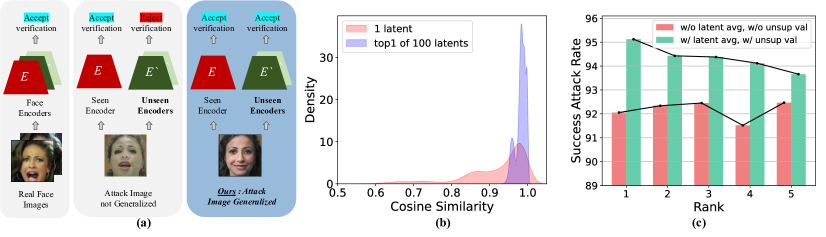
Figure 1: (a) Poorly generalized attack images often get rejected on unseen encoders (middle) while generalized images can bypass other unseen systems (right) like real face images (left).(b) Cosine similarity when only one latent is optimized (red) and the top 1 of when multiple latents are optimized (blue). Red histogram suffers with underfitting. (c) SAR of top 1 to 5 candidates tested on unseen encoders of target encoder (coral bar) and our method (turquoise bar). Our method shows consistent correlation between rank and performance as well as better results.

1 Introduction

With the increasing deployment of face recognition systems in security-critical environments, threat actors are developing sophisticated attack strategies over various attack points, where one of the major threats is face reconstruction attacks [18, 6, 7, 23, 24, 8]. The primary goal of face reconstruction attacks is to create fake biometric images that resemble genuine ones from the stored biometric templates which are then used to bypass the system. Previous works have mostly focused solely on attacking the target (seen) encoder, i.e., using these fake biometric images to bypass the same system. However, transfer attack scenarios, where these fake biometric images are used to bypass other unseen systems (Fig. 1a middle) are not discussed enough. They are potentially more perilous than common attacks as they can break into a wide range of face recognition systems.

Formally, we define Face Reconstruction Transfer Attacks (FRTA) as successfully reconstructing a face image that can substitute a real face image on unseen encoders, as illustrated in Fig 1a. To state our problem in a rigorous and tractable framework, we formulate this task to reconstruct a face image which matches the original image in identity by a finite number of unseen face encoders given only a single encoder and a feature embedded through this encoder (section 3). However, existing works do not consider transfer attacks in their designs thoroughly.

To solve FRTA effectively, we first devise a novel out-of-distribution (OOD) oriented FRTA framework that reformulates the attack as a problem of generalization of loss function over OOD of network parameters. Our FRTA task falls to the standard OOD generalization category in that the loss function needs to be optimized by one variable and generalized with respect to the other instantiated from unseen distributions. We postulate a white-box scenario where a single encoder and a template feature embedded through this encoder are given and face reconstruction is achieved by optimizing the data input in a way to minimize feature reconstruction loss. Instead of directly updating the input image, we adopt a generative model and update its latent which outputs an image(Fig. 2 step 1).

However, reconstructing the face with naive latent optimization is likely to suffer from underfitting with poor latent optimizations (Fig. 1b red histogram). To address this challenge, we introduce an Averaged Latent Search with Unsupervised Validation through pseudo target (ALSUV) framework, which is motivated by the OOD generalization concept. In this OOD-oriented approach, we 1) optimize multiple latents concurrently by 2) employing latent averaging and 3) searching for the most optimal generalized sample through unsupervised validation using a validation encoder. Multiple latent optimization prevents poor optimization by selecting the well-optimized sample close to the target(Fig. 1b blue histogram). However, this potentially causes overfitting to the seen encoder (Fig. 1c coral bars). Therefore, we average latents throughout optimization trajectories which provides a flatter loss surface (Fig. 4) and leads to OOD generalization [21, 3, 22]. Additionally, we adopt an unsupervised validation search with pseudo target, which incorporates a surrogate validation encoder to search for the best generalizing sample in validation encoder space. Overall, latent averaging and unsupervised validation alleviate overfitting to seen encoder as shown in Fig. 1c (turquoise bar) where rank and performance are notably correlated.

Contributions

The contributions of our work are summarized as:

• We address FRTA as a threat that can potentially bypass a wide range of unseen face recognition systems. We rigorously formulate the reconstruction problem as an OOD generalization problem and enhance the attack performance with a multiple latents optimization strategy. To address overfitting, we introduce the OOD-oriented ALSUV, which includes latent averaging and unsupervised validation using pseudo targets from a validation encoder.

• Our method achieves state-of-the-art in face reconstruction transfer attack tested on a subset of LFW, CFP-FP, and AgeDB datasets with 6 different types of face encoders in terms of conventionally used success attack rate and top-1 identification rate where we are the first to attempt.

• We comprehensively examine our method through ablation study, hyperparameter analysis, and evaluate the image quality. Also, we conduct additional experiments to analyze the effect of optimizing multiple latents, latent averaging, and unsupervised validation.

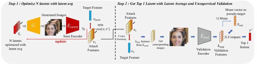
Figure 2: Overview of our method. Latents of a pre-trained generative model $G$ is optimized to ensure high similarity between the feature embedding of reconstructed samples and real feature embeddings.

2 Related Works

2.1 Face Reconstruction from Features

NBNet [18] first pioneered face reconstruction from the template by neighborly deconvolution, but the results are substandard for both quality and performance. [6] projects features into the latent space of a pre-trained StyleGAN2 [14] to generate fine-grained resembling images. The results are qualitatively decent, but often contain different identities as shown in Fig. 6. DiBiGAN [8] presents a generative framework based on bijective metric learning and pairs features with face images one-to-one. These methods offer fast sample generation after training but require extensive face datasets and time for training a new network. [23] samples varying random Gaussian blobs iteratively and combining the blobs as the shape of a face. It requires only a few queries and no prior knowledge such as dataset, but shows results with low quality. [24] reconstructs faces using similarity scores based on eigenface with soft symmetry constraints, generative regularization, and multi-start policy to avoid local minimas. However, the reconstructed images show severe noise as shown in Fig. 6. These works consume less time to generate few samples than training a new network but takes longer for large scale generations.

Methods introduced above show promising results when tested with seen encoders, but performance drastically falls with unseen encoders. Recently, a couple of works [7, 19, 27] considered FRTA scenarios in their work. [7] suggests a genetic algorithm-based approach along with an attack pipeline to impersonate the target user. Reconstructed images are high quality, but evolutionary algorithms rely on random mutation and selection processes which might get trapped in local optima or fail to generalize well due to the limited exploration-exploitation trade-off inherent in their design. [19] suggests query efficient zeroth-order gradient estimation with top $k$ initialization search followed by ensembling. This approach typically iteratively adjusts latent representations to minimize reconstruction errors but may suffer from overfitting to specific characteristics of the seen encoder. [27] trains a network which maps features to the $\mathcal{W^{+}}$ latent space of StyleGAN3 to learn the $\mathcal{W^{+}}$ distribution space based on a WGAN framework, however, the GAN frameworks are prone to mode collapse.

2.2 Out-of-Distribution Generalization

Generalization is one of the most important tasks in deep learning models especially when it comes to unseen OOD circumstances. Searching for flat minima is one of the main stems of research to achieve generalization where [21] establishes a strong connection between the flatness of the loss surface and generalization in deep neural networks. Weight averaging[9, 13, 3, 22, 21] ensembles the trajectories of non-linear function parameters during training to seek well generalized flat minima point. [9] gathers information from separately trained models, [13] stochastically averages a single model with cyclic learning rate, [3] aggregates from a dense trajectory, and [22] collects from several different training policies. Our task focuses on generalizing reconstructed face over unseen encoders, hence, we adopt the core principles from these works and adequately modify them for our work.

Pseudo label has been used for generalization tasks where label information is scarce such as domain adaptation[25, 28, 36]. They can be made by mixing both samples and labels[35], ensembling labels from augmented samples [1, 12], or confidence prediction with sliding window voting followed by confidence-based prediction[28]. The key components for pseudo labels are sufficiently high confidence [12, 28] and adequate regularization to prevent over-confidence[36, 37]. Our method requires selecting the best generalizing input(latent) in an unsupervised manner. Hence, we migrate the idea of previous works and discover how to find the proper pseudo target for our task.

3 Face Reconstruction Transfer Attack as OOD Generalization

We first clearly define the problem of FRTA, and we show that face reconstruction transfer attack is in fact an OOD generalization problem.

3.1 Problem Formalization

The FRTA can be formalized as an algorithm $\mathcal{A}$ that must return a solution vector $\mathcal{A}(\theta_{seen})=x^{*}$ to the following optimization objective:

$$\max_{x}\min_{\theta\in\Theta}sim(E_{\theta}(x),v_{\theta}),$$ (1)

where $v_{\theta}$ indicates a true target $v_{\theta}=E_{\theta}(x_{real})$ corresponding to an encoder $E_{\theta}$. The nature of FRTA poses a constraint that the attacker can access to the seen encoder $E_{\theta_{seen}}$ only. The encoder parameter space $\Theta$ includes both seen and unseen encoder networks exposed to attacks. Hence, the objective requires that the attack must be transferrable.

One approach to the attack is by using a face image generator $G$. By substituting $x=G(z)$ in the above equation, one maximizes the objective in terms of $z$ instead of $x$ as:

$$\max_{z}\min_{\theta\in\Theta}sim(E_{\theta}(G(z)),v_{\theta}).$$ (2)

3.2 FRTA As OOD Generalization

Given that both $E_{\theta}$ and $G$ are multi-layer perceptron instances, we show that the FRTA can be formulated as an OOD generalization problem. To this end, we first formalize the OOD generalization as follows:

Definition. OOD generalization on the domain $\mathcal{D}$ in the parameter space $\Theta$ is to solve for an algorithm $\mathcal{A}$ that, given a seen dataset, returns a solution parameter $\mathcal{A}(D_{seen})=\theta^{*}$ that minimizes

$$\min_{\theta}\max_{D\in\mathcal{D}}L(\theta;D),$$ (3)

where $L$ is a loss function defined as

$$L(\theta;D)=\frac{1}{\left|D\right|}\sum_{(x,y)\in D}l(f_{\theta}(x),y).$$ (4)

Here, $f_{\theta}$ is an MLP parametrized by $\theta$, and $l$ is a sample-wise loss function on a label-data pair. ∎

Theorem. Define $f_{z}$ by $f_{z}(\theta)=E_{\theta}(G(z))$, and let $D^{*}_{seen}=\{(\theta_{seen},v_{\theta_{seen}})\}$, $\mathcal{D}^{*}=\{\{(\theta,v_{\theta})\}:\theta\in\Theta\}$, and

$$l(f_{z}(\theta),v_{\theta})=-sim(f_{z}(\theta),v_{\theta}).$$ (5)

Then, $f_{z}$ is an MLP, and the FRTA algorithm $\mathcal{A}$ on $\Theta$ is an OOD generalization algorithm $\mathcal{A}^{*}$ on the domain $\mathcal{D}^{*}$ in the parameter space $\mathcal{Z}$.

The theorem is proved (in Supp. 0.A) by observing the duality between data and parameter; in MLP, data can be viewed as parameter, and vice versa.

3.3 Averaged Latent Search with Unsupervised Validation with Pseudo Target(ALSUV)

Inspired by the above interpretation, we tackle FRTA by means of OOD generalization techniques by defining the similarity as a loss function. Thereupon, we propose ALSUV with pseudo target, which is an integrated approach of OOD generalization on the latent.

The latent search mechanism of ALSUV are decomposed as follows: (1) multiple latent optimization, (2) latent averaging throughout optimization trajectories, and (3) unsupervised validation with the pseudo target.

3.3.1 Multiple Latent Optimization

In order to avoid the underminimization problem shown in Fig. 1b and to generate candidates for our following unsupervised validation method, we initialize multiple $n$ latent vectors and optimize them in a parallel manner:

$$\underset{\{z_{i}\}_{i=1}^{n}}{\min}\,\sum_{i=1}^{n}L(z_{i};E_{seen})=-\sum_{i=1}^{n}sim(E_{seen}(G(z_{i})),v_{seen})$$ (6)

where $E_{seen}=E_{\theta_{seen}}$ $v_{seen}=v_{\theta_{seen}}$. The given loss function is minimized by a gradient-based update using the standard optimizer such as Adam[15] or SGD. Fig. 3 validates that updating with multiple latents significantly improves the minimization of the loss. Moreover, we find that this simple multiple latent optimization can more effectively escape from poor local minima than iterating with complicated learning rate scheduler (Tab. 6).

3.3.2 Latent Averaging

Avoiding the poor underminimization issue alone is not sufficient for effective generalization of the attack under FRTA since the acquired solution may overfit to seen encoders as shown in Fig. 1c. To effectively improve the attack rate on the unseen encoders, we borrow the idea from OOD generalization[21, 3, 22] and apply averaging the solution latent vectors over the optimization trajectory:

$$\overline{z}_{i}=\frac{1}{T_{0}}\sum_{t=T-T_{0}}^{T}z^{(t)}_{i}$$ (7)

where $z^{(t)}_{i}$ are the latent vectors acquired at step $t$ of the optimization of Eq. (6), $T$ is the total number of optimization steps, and $T_{0}$ is the size of steps to average the latent vectors.

Due to the equivalence between FRTA and OOD generalization (Thm. LABEL:thm:taood), latent averaging can improve the generalization of the similarity maximization under unseen encoder networks and corresponding unseen targets. Fig. 3 evidences our hypothesis, indicating that averaging the latents improves the attack rate on the unseen encoders. Moreover, Fig. 4 shows that latent averaging improves the transfer attack by smoothening the loss surface of our objective, validating the equivalence between OOD generalization and FRTA.

3.3.3 Unsupervised Validation with Pseudo Target

Despite its effectiveness, multiple latent optimizations with averaging can still suffer overfitting issues as no explicit information of unseen encoders is exposed to the optimization. Therefore, we acquire more explicit information of unseen encoders by utilizing a surrogate validation encoder $E_{val}=E_{\theta_{val}}$. Particularly, we propose to validate our reconstruction criterion Eq. (1) over the surrogate validation encoder. One remaining issue however is the absence of validation target vector $v_{val}$. To resolve it, we construct the pseudo target:

$$\widehat{v}_{val}=\frac{1}{k_{top}}\sum_{i=1}^{k_{top}}E_{\theta_{val}}(G(\overline{z}_{(i)})),$$ (8)

by averaging the reconstructed features from the top $k$ latent vectors of the attack objective in Eq. (6). Namely, $\overline{z}_{(i)}$ are ordered with respect to the similarity to the seen feature $L(\overline{z}_{(1)})\leq\dots\leq L(\overline{z}_{(n)})$. The pseudo target may not be fully precise approximation of validation target $v_{val}$ from the real ground truth image. However, we show that it improves the attack under FRTA by mitigating the overfitting issue of the latent optimization (Fig. 3c). Moreover, we find that the average of multiple top $k$ reconstructed features better serves as an alternative of $v_{val}$ than the single top $1$ feature as the latter may have been overfitted to the seen target.

3.3.4 Full Objective

Overall, the ALSUV algorithm searches the solution latent $z^{*}$ by unsupervised validation

$$z^{*}=\arg\min_{\overline{z}_{i}}d(E_{val}(G(\overline{z}_{i})),\widehat{v}_{val}),$$ (9)

subject to $\overline{z}_{i}\in S$ within the search space $S$ of multiple latent-averaged vectors defined in Eqs. (6) and (7) based on a pseudo target $\widehat{v}_{val}$ defined in Eq. (8). The reconstruction target feature of ALSUV avoids under-minimization of latent optimization, thereby effectively attacking the seen encoder. On the other hand, it achieves robust FRTA based on latent averaging and validation against pseudo target with the surrogate validation encoder. The full algorithm is given in Supp. 0.B.

4 Experiments

The experiments section includes: 1) performance evaluation against existing methods; 2) comprehensive component ablation and hyperparameter variation to show effectiveness; 3) analysis of components by varying setups, comparing parallel latent optimization to serial optimization, visualizing loss surface effects with and without latent averaging, using different validation encoders for unsupervised validation, and assessing image quality visually and quantitatively.

4.1 Configuration

We use StyleGAN2[14] trained with FFHQ-256 for the generative model, denoted as $G(\cdot)$, and latents are optimized in the $\mathcal{W^{+}}$ space. Both $G(\cdot)$ and target encoders $E_{seen}(\cdot)$ are frozen while optimizing latents. We adopt Adam[15] optimizer with 100 steps where the learning rate starts from 0.1 and is divided by 10 at iteration 50. Our method involves three hyperparameters: $n=100$, the number of latents; $t=70$, length of trajectory for latent averaging; and $k_{top}=10$, the number of samples used for unsupervised validation. We use pytorch[20] for all experiments on a single Nvidia RTX 2080ti GPU.

Table 1: Success Attack Rate (SAR) of previous works and our proposed method. Red colored cells indicate results of seen encoder setup. We highlight our method with grey and best results are highlighted with bold.

Dataset		LFW							CFP-FP							AgeDB-30
Test Encoder		FaceNet	MobFace	ResNet50	ResNet100	Swin-S	VGGNet	Unseen AVG	FaceNet	MobFace	ResNet50	ResNet100	Swin-S	VGGNet	Unseen AVG	FaceNet	MobFace	ResNet50	ResNet100	Swin-S	VGGNet	Unseen AVG
Target Encoder	Real Face	99.87	99.83	99.83	99.93	99.93	99.8	-	93.85	76.15	95.38	95.38	90	93.08	-	92.63	93.53	92.34	97.17	96.23	91.7	-
FaceNet	NBNet	82.91	0.57	70.58	34.85	0.74	74.15	36.51	80.77	25.38	73.85	36.15	18.46	73.08	47.69	69.91	2.57	63.69	19.57	2.7	60.99	32.49
	LatentMap	60.28	5.33	53.76	4.52	8.4	59.47	31.74	49.23	21.54	36.15	13.08	44.62	41.54	35.96	49.53	8.05	35.37	1.61	3.51	39.97	21.73
	Genetic	87.72	8.5	63.52	7.46	16.1	76.04	34.32	80.77	26.92	58.46	25.38	39.23	54.62	40.92	66.82	9.04	46.31	7.05	7.98	49.76	24.03
	GaussBlob	0.4	0.2	0.03	0	0	2.8	0.61	9.23	6.92	10	1.54	6.15	9.23	6.77	6.15	3.7	11.59	0.39	1.32	14.29	6.26
	EigenFace	91.46	17.82	56.67	24.6	21.77	69.59	38.09	13.08	26.92	58.46	19.23	33.85	60	39.69	16.96	9.49	53.14	8.79	3.96	55.71	26.22
	FaceTI	3.4	2.06	4.15	0.3	0.57	8.46	3.11	84.62	26.92	58.46	19.23	33.85	60	39.69	73.87	9.49	53.14	8.79	3.96	55.71	26.22
	QEZOGE	99.6	25.95	93.29	59.72	67.85	96.39	68.64	91.54	39.23	83.85	58.46	67.69	77.69	65.38	88.12	19.99	72.42	31.09	24.59	79.08	45.43
	Ours	99.83	65.15	97.51	86.79	83.32	99.22	86.4	94.62	46.15	86.15	73.08	73.85	86.15	73.08	89.67	30.8	79.18	48.89	38.46	83.39	56.14
MobFaceNet	NBNet	4.52	30.17	2.56	2.36	3.44	7.41	4.06	12.31	49.23	18.46	9.23	16.15	10	13.23	13.32	21.15	12.58	4.06	2.32	16.7	9.8
	LatentMap	4.18	7.12	7.96	0.88	2.29	8.61	4.78	13.85	14.62	17.69	1.54	12.31	15.38	12.15	11.91	6.63	12.42	0.74	1.64	14.23	8.19
	Genetic	13.87	49.54	15.05	4.42	8.17	18.8	12.06	23.08	45.38	26.92	13.85	28.46	28.46	24.15	19.31	33.02	19.76	3.57	5.31	20.86	13.76
	GaussBlob	2.97	75.57	3.37	4.62	6.61	7.29	4.97	11.54	61.54	13.85	3.85	10.77	13.85	10.77	11.43	45.25	8.24	6.28	4.63	13.81	8.88
	EigenFace	62.44	99.39	63.45	56.87	75.26	65.54	64.71	51.54	70.77	59.23	47.69	64.62	54.62	55.54	59.51	88.86	51.66	35.66	40.88	56.32	48.81
	FaceTI	15.67	21.91	18.2	4.55	9.81	24.5	14.55	19.23	23.08	23.85	6.92	13.85	21.54	17.08	29.51	14	24.46	3.35	4.6	28.52	18.09
	QEZOGE	61.51	97.98	67.81	54.36	65.28	69.87	63.77	39.23	70.77	44.62	32.31	49.23	43.08	41.69	50.98	79.76	52.04	30.35	34.15	56	44.7
	Ours	96.76	99.83	97.3	96.83	99.16	98.05	97.62	80	79.23	81.54	84.62	83.85	83.85	82.77	85.1	93.72	84.68	87.93	87.58	86.22	86.3
ResNet50	NBNet	61.09	1.79	84.68	34.12	0.3	78.1	35.08	64.62	23.85	77.69	46.92	14.62	66.92	43.39	68.62	4.31	76.67	31.12	1.71	72.55	35.66
	LatentMap	24.97	5.7	29.67	2.36	9.11	33.68	15.16	33.08	16.15	28.46	7.69	19.23	30.77	21.38	30.25	4.57	29.61	1.71	2.22	30.96	13.94
	Genetic	61.09	12.55	83.46	8.2	13.7	72.53	33.61	49.23	19.23	60.77	20.77	40	49.23	35.69	46.64	10.04	60.32	7.76	8.34	50.02	24.56
	GaussBlob	0.03	0.1	0.2	0	0	0.4	0.11	3.08	22.31	6.15	1.54	2.31	6.15	7.08	2.67	1.32	4.18	0.29	0.29	4.92	1.9
	EigenFace	78.87	35.3	95.75	47.69	48.8	84.48	59.03	70	38.46	81.54	51.54	45.38	78.46	56.77	69.04	19.83	81.14	25.1	26.62	73.32	42.78
	FaceTI	12.87	8.93	18.77	1.58	4.31	21.27	9.79	20.77	13.08	23.08	6.15	16.15	21.54	15.54	32.99	11.3	28.23	2.45	3.54	31.61	16.38
	QEZOGE	86.01	42.97	98.31	68.32	64.34	90.06	70.34	73.85	39.23	86.92	53.85	63.08	73.85	60.77	71.26	20.05	85.48	35.66	27.39	77.02	46.28
	Ours	99.12	85.24	99.8	97.44	97.61	99.63	95.81	89.23	65.38	95.38	82.31	84.62	86.92	81.69	88.86	56.2	91.6	76.6	71.32	89.28	76.45
ResNet100	NBNet	20.18	4.08	28.35	48.36	8.98	30.1	18.34	33.08	27.69	41.54	51.54	28.46	46.15	35.38	37.66	8.43	48.41	62.92	16.83	47.67	31.8
	LatentMap	6.68	3.27	7.69	3.04	3.61	11.81	6.61	20	15.38	16.92	12.31	21.54	23.08	19.38	6.57	3.22	8.24	1.09	0.68	9.56	5.654
	Genetic	23.42	9.55	25.31	47.76	15.22	29.97	20.69	41.54	28.46	35.38	48.46	41.54	33.08	36	23.79	9.69	21.98	38.56	10.75	24.2	18.08
	GaussBlob	31.7	51.86	60.7	85.52	71.3	48.72	52.86	35.38	21.54	43.85	61.54	45.38	40.77	37.38	50	35.83	52.29	73.63	50.76	54.32	48.64
	EigenFace	85.69	69.96	87.61	95.41	91.33	87.24	84.37	65.38	45.38	63.85	85.38	78.46	63.08	63.23	79.11	52.4	81.88	93.24	81.2	80.08	74.93
	FaceTI	15.57	38.22	21.47	39.33	29.29	28.95	26.7	28.46	36.92	42.31	45.38	50.77	40.77	39.85	20.12	29.87	26.39	37.88	23.46	31.19	26.21
	QEZOGE	55.88	48.57	69.94	98.89	73.78	71.39	63.91	53.08	40.77	53.85	86.15	64.62	55.38	53.54	47.51	25.59	50.53	91.37	45.38	54.84	44.77
	Ours	99.36	96.16	99.56	99.93	99.93	99.56	98.91	91.54	67.69	95.38	95.38	90	90	86.92	92.11	85.07	91.73	97.01	94.85	91.76	91.1
Swin-S	NBNet	12.76	7.19	15.79	16.67	9.65	16.4	13.76	23.85	26.15	35.38	29.23	30.77	28.46	28.61	41.65	11.01	44	36.34	25.01	43.16	35.23
	LatentMap	3.61	1.08	3.88	0.4	1.28	6.14	3.02	16.15	16.15	15.38	3.08	19.23	16.92	13.54	8.27	2.32	8.72	0.9	1.19	9.85	6.01
	Genetic	35.61	21.03	39.39	12.66	51.3	45.9	30.92	45.38	33.08	37.69	29.23	65.38	35.38	36.15	30.87	12.78	28.26	11.39	26.52	29.42	22.54
	GaussBlob	0.2	3.51	0.37	1.21	5.4	0.34	1.13	10	27.69	11.54	5.38	20	6.92	12.31	5.28	7.82	8.72	4.22	6.12	9.72	7.15
	EigenFace	17.48	50.46	33.24	30.88	56.94	65.49	56.45	35.38	34.62	36.15	20.77	50	43.85	44.31	37.59	30.13	36.21	20.6	23.82	39.27	32.76
	FaceTI	51.9	65.15	59.82	39.87	61.61	37.9	33.99	43.08	46.15	44.62	43.85	58.46	33.08	32	40.88	29.39	42.26	16.99	39.97	38.91	33.69
	QEZOGE	78.7	66.94	84.33	80.59	97.44	86.52	79.42	67.69	50	69.23	65.38	81.54	72.31	64.92	59.54	32.76	57.45	55.17	83.13	61.15	53.21
	Ours	98.08	99.02	99.02	99.87	99.93	99.36	99.07	87.69	73.08	89.23	93.08	90.77	88.46	86.31	89.35	87.19	89.15	95.72	96.3	90.15	90.31
VGGNet	NBNet	45.57	1.38	63.5	16.51	2.39	73.78	25.87	56.15	22.31	65.38	37.69	24.62	69.23	41.23	63.05	3.89	67.46	21.63	4.25	70.49	32.06
	LatentMap	21.13	3.78	32.3	2.5	2.77	38.34	12.5	28.46	13.08	26.15	7.69	20	28.46	19.08	22.01	4.8	23.88	0.74	1.51	29.77	10.59
	Genetic	60.01	9.21	66.05	9.58	13.36	85.29	31.64	50	21.54	52.31	21.54	33.08	61.54	35.69	45.38	7.53	40.49	3.7	4.67	55.75	20.35
	GaussBlob	0.4	0.07	0.3	0	0	3	0.15	0.67	21.54	6.92	0.77	2.31	8.46	6.44	6.03	0.92	4.53	0.2	0	11.74	2.34
	EigenFace	93.82	25.99	93.93	44.52	57.21	99.12	63.09	84.62	37.69	86.15	62.31	60	89.23	66.15	72.67	14.55	72.55	18.44	15.45	81.2	38.73
	FaceTI	2.36	2.46	2.46	0.3	1.28	7.41	1.77	7.69	6.15	9.23	0.77	7.69	13.85	6.31	25.04	6.76	17.25	1.09	3.06	23.98	10.64
	QEZOGE	90.26	47.32	91.64	64.54	60.57	98.69	70.87	77.69	43.85	79.23	60	65.38	88.46	65.23	73.9	19.76	75.12	28.71	25.43	85.9	44.58
	Ours	99.29	77.45	99.49	94.57	93.9	99.8	92.94	89.23	63.85	90.77	87.69	85.38	91.54	83.38	83.97	37.4	83.55	55.62	47.38	89.25	61.58

Table 2: Rank 1 identification rate of previous works and our proposed method. Red colored cells indicate results of seen encoder setup. We highlight our method with grey and best results are highlighted with bold.

Datsaet		LFW							CFP-FP							AgeDB-30
Test Encoder		FaceNet	MobFace	ResNet50	ResNet100	Swin-S	VGGNet	Unseen AVG	FaceNet	MobFace	ResNet50	ResNet100	Swin-S	VGGNet	Unseen AVG	FaceNet	MobFace	ResNet50	ResNet100	Swin-S	VGGNet	Unseen AVG
Target Encoder	Real Face	99	99.5	99.5	99.5	99.5	99.5	-	95.5	88.5	93.5	100	99	94	-	92	96	92.5	98	98	87.5	-
FaceNet	NBNet	86.07	1	57.71	39.3	3.48	53.23	30.94	62	1.0	46.5	38.5	5	50	28.3	92.5	0	56	21.5	3.5	60	28.2
	LatentMap	32.5	2	20	12.5	11.5	19.5	13.1	17.5	1.5	14	10	8	13	9.3	15.5	1.5	7	2	2	7.5	4
	Genetic	82.5	7.5	39	18.5	23	39	25.4	18	3	15.5	11.5	10.5	18	11.7	43	1.5	14.5	6.5	4	17.5	8.8
	GaussBlob	0.5	0.5	0	0	0	0	0.1	1	0.5	1	1	0	0.5	0.6	0.5	0	0	0	0	0	0
	EigenFace	91.54	13.93	48.26	30.35	17.91	51.24	32.34	72	2	39.5	17.5	8	34	20.2	69.5	3	23	6.5	7.5	30.5	14.1
	FaceTI	1	0	0	1	0.5	2.49	0.8	0.5	0.5	1.5	0	0	0.5	0.5	0.5	0	0.5	0.5	0.5	0.5	0.4
	QEZOGE	100	25.37	90.55	77.61	69.15	94.03	71.34	91	16	66	65	52	73.5	54.5	96	9.5	59.5	33	26	70	39.6
	Ours	100	55.5	100	94.53	91	100	88.21	95.5	21	79.5	81	63.5	85	66	98	21.5	80.5	56	45.5	87.5	58.2
MobFace	NBNet	1.49	47.76	1	12.44	8.45	4.98	5.67	0.5	4.5	2.5	5	2	2.5	2.5	2	41.5	2	13	7.5	3.5	5.6
	LatentMap	3.48	4.48	2.49	1.99	1.49	1.49	2.19	3	1	1.5	1	3	2.5	2.2	0	3.5	1	0.5	1	2	0.9
	Genetic	2.99	68.66	7.46	6.97	9.95	6.47	6.77	6.5	5	3	3.5	5	5.5	4.7	2.5	53	5	3.5	2.5	7	4.1
	GaussBlob	0	89.05	2.99	25.87	21.89	3.98	10.95	3	10	1.5	6	2.5	2	3	1.5	81.5	1.5	16	15.5	1.5	7.2
	EigenFace	46.27	100	55.22	74.13	90.05	52.74	63.68	30.5	76	37.5	46	56.5	33.5	40.8	33	99.5	38	54	77.5	43	49.1
	FaceTI	10.45	17.41	8.96	9.45	12.44	8.96	10.05	7.5	8	5.5	8.5	7	6	6.9	4	7.5	4	3.5	4	2.5	3.6
	QEZOGE	38.81	100	47.76	59.7	65.67	45.77	51.54	22	60.5	27.5	46.5	40.5	25.5	32.4	24	99.5	28.5	43	50	29.5	35
	Ours	94.5	100	99	99.5	100	98.5	98.3	75.5	87	78.5	92.5	94	78	83.7	92.5	99.5	97	97	98.5	94	95.8
ResNet50	NBNet	60.5	0.5	88.5	53.5	3	60.5	35.6	48	0.5	61	43	3.5	50	29	65	0.5	95	40.5	5.5	76	37.5
	LatentMap	9	2.5	12.5	2.36	9.5	14.5	7.57	9	2	11.5	11.5	7	10.5	8	5	2	13.5	3	3	8	4.2
	Genetic	29	5.5	80.5	18	16.5	47	23.2	16	3	23.5	14.5	11	12	11.3	15.5	4	65.5	5	7.5	23.5	11.1
	GaussBlob	0	0	0	0	0	0	0	0.5	0	0	0	0.5	0.5	0.3	0	0.5	0	0.5	1	0.5	0.5
	EigenFace	69.15	29.35	99	65.67	67.16	81.59	62.58	50	7	74.5	49.5	32	60.5	39.8	55	24	99	43	45	79	49.2
	FaceTI	5.47	3.48	6.97	3.48	4.98	6.47	4.78	4	2.5	5.5	5.5	6	4.5	4.5	3.5	1.5	6	3	1	5	2.8
	QEZOGE	79.6	31.84	100	75.12	67.16	88.06	68.36	63.5	19.5	83	64	53.5	64.5	53	66.5	12.5	100	47	31	82.5	47.9
	Ours	100	90	100	100	99	100	97.8	91.5	52	94	95.5	86.5	89	82.9	98	74	100	89.5	85	99.5	89.2
ResNet100	NBNet	21	7	31	91	26.5	20	21.1	11	0.5	19.5	57.5	11	19	12.2	18.5	2.5	24	91	33	18	19.2
	LatentMap	3.48	1.49	2.49	6.47	4.98	2.99	3.09	6	2.5	5.5	11.5	7.5	7	5.7	1.5	0	0.5	1.5	0	0	0.4
	Genetic	14.43	6.97	12.94	75.12	25.37	14.93	14.93	7.5	4	6	24	8.5	6.5	6.5	4	0.5	3	70.5	8.5	4	4
	GaussBlob	34.5	52	51.5	90	75.5	46	51.9	17.5	8.5	29.5	70.5	38.5	23.5	23.5	20.19	39.42	32.69	89.42	71.15	25	37.69
	EigenFace	76.12	79.6	85.07	99.5	96.52	78.11	83.08	54.5	23.5	65.5	95.5	85	56.5	57	57	67	66.5	98.5	96	61.5	69.6
	FaceTI	16.42	35.32	19.9	70.65	39.3	16.92	25.57	16	24.5	18	55	32	19	21.9	7.5	12	7.5	63	22.5	7	11.3
	QEZOGE	50.75	34.83	48.26	100	71.14	51.74	51.34	44	17	49.5	97	61	47	43.7	16.5	10.5	27	99	52.5	19	25.1
	Ours	99.5	99.5	99.5	100	100	98.51	99.4	89	70.5	92	100	98	90.5	88	86	86	91.5	100	99	88.5	90.2
Swin-S	NBNet	14.5	8	20	47	39.5	15.5	21	12.5	1	14.5	29	13	10.5	13.5	20.5	6	24	57.5	58.5	16	24.8
	LatentMap	2	0.5	3.5	1.5	1.5	3.5	2.2	3.5	1.5	2.5	6	5	3.5	3.4	0	0	0	0	2.5	0	0
	Genetic	15.5	9	17	27.5	67	19	17.6	9	3	7.5	9.5	18	8	7.4	6.5	4.5	4.5	13.5	52.49	4	6.6
	GaussBlob	0	3.98	0	7.46	22.89	0	2.29	0	1.5	1	4	6.5	0.5	1.4	1	5.5	1	10.5	16.5	1.5	3.9
	EigenFace	9.95	59.2	17.41	46.27	75.62	16.92	29.95	7.5	12.5	13.5	22.5	40.5	13	13.8	8	45	13.5	34.5	69.5	13.5	22.9
	FaceTI	35.82	55.22	36.32	50.25	63.18	34.83	42.49	28	30.5	32	44	46	27.5	32.4	13	20	8.5	21	31	11.5	14.8
	QEZOGE	57.71	57.21	67.16	87.56	100	64.68	66.86	44	29.5	49	78.5	90	52	50.6	23	20	28	68	95.5	18.5	31.5
	Ours	98.5	100	100	100	100	99.5	99.6	80	77.5	83	99.5	99	83	84.6	80.5	94.5	89.5	99.5	100	86.5	90.1
VGGNet	NBNet	48.76	1.99	59.7	38.81	9.95	70.15	31.84	45.5	1	49	36.5	8.5	48.5	28.1	61.5	0.5	71.5	35.5	7	88.5	35.2
	LatentMap	7	1.5	9	5	4	11	5.3	7.5	0.5	9	3.5	4.5	10	5	3.5	0.5	5.5	0.5	0.5	3.5	2.1
	Genetic	37.5	6	43	21.5	16	71.5	24.8	16.5	1	16.5	10	9.5	21.5	10.7	17	1.5	19	4	4	42	9.1
	GaussBlob	0	0	0	0	0	1.99	0	0.5	0	1	0	0	1.5	0.3	0.51	0	1.02	0	0	1.53	0.306
	EigenFace	92.54	36.32	92.54	73.13	73.13	99.5	73.53	74.5	11	73.5	64	48.5	88.5	54.3	74	15.5	80.5	29	27	93.5	45.2
	FaceTI	1.49	2.49	2.99	1.99	1.49	3.98	2.09	3	2	4.5	2	2	4.5	2.7	1.5	0.5	1.5	0.5	1	1.5	1
	QEZOGE	91.54	39.3	93.53	76.12	75.12	99	75.12	72.5	16.5	72	70	55	84.5	57.2	72	13	76	35.5	26	96	44.5
	Ours	99.5	82	100	99	99	100	95.9	90	34	88.5	93	84.5	93.5	78	92.5	43	93.5	68	64.5	98.5	72.3

4.2 Datasets and Networks

We use the LFW, CFP-FP, and AgeDB-30 datasets, three widely used verification datasets with distinct characteristics. For LFW and AgeDB-30, we compare reconstructed samples with every other positive sample except the one used for reconstruction, resulting in 3,166 and 3,307 pairs of comparisons, respectively. CFP-FP consists of frontal and profile images; we reconstruct only the frontal images and follow the challenging frontal-profile verification protocol, resulting in 130 pairs in total (not all sampled identities were used in the given protocol). For identification, we set up generated samples as probes and every image as the gallery, resulting in 13,233, 2,000, and 5,298 samples in the gallery, respectively, consisting of 5,749, 500, and 388 identities for LFW, CFP-FP, and AgeDB-30, respectively. For CFP-FP, we use generated frontal images for probes and profile images for the gallery, which is very challenging. We randomly sample 200 non-overlapping identities each from 3 datasets. We use encoders based on various backbones which are equipped with different classification heads and distinct datasets. Specific configurations are shown in Supp. 0.D Tab. 8. For the validation encoder, we use Swin-T as the default.

4.3 Evaluation Metrics and Details

[18] introduces Type I and Type II SAR where Type I compares the generated face with the ground truth target, while Type II compares with different images from the same identity. SAR measures the ratio of generated samples passing the positive verification test where thresholds are specific to type of datasets and face encoders. Since Type I is relatively easy, we only report Type II performance which is more challenging. We also evaluate identification rate, where we retrieve the top 1 sample from gallery composed of real samples and probes consisting of generated samples. We include target samples in the gallery which is still challenging. In ablation, we also report the SAR@FAR which is the success attack rate at thresholds of FAR($=1e-4,1e-3,1-e2$).

4.4 Comparison with Previous Works

We compare our method with state-of-the-art feature-based face reconstruction methods including NBNet [18], LatentMap [6], Genetic [7], GaussBlob [23], Eigenface [24], FaceTI [27], and QEZOGE [19]. For FaceTI [27], we used StyleGAN2 and our face encoders for reproduction. As shown in Tab. 1 and Tab. 2, overall previous methods are effective on seen encoders, but the performance drastically drops on unseen encoders. EigenFace [24], FaceTI [27], and QEZOGE [19] show better performance compared with other works, however, tend to show lower performance compared with our method and the results highly fluctuates depending on the type of seen encoder. In contrast, our method outperforms for both seen and unseen cases. Our SAR and identification rate results are close to real face images on seen encoders while outperforming previous works with a large margin on unseen encoders for every dataset while depending less on the type of seen encoder. Additionally, results tested on unseen encoders shown in Tab. 1 and Tab. 2 present that our method achieves OOD generalization on unseen encoders successfully.

Table 3: Ablation study controlling the components of our suggested method. Performance is averaged over the test results on unseen encoders with SAR@FAR$(=1e-4,1e-3,1e-2)$ and SAR$(score\geq threshold)$ for each of the datasets respectively. Best results are highlighted in bold.

Dataset			LFW				CFP-FP				AgeDB-30
Metric			SAR@FAR			SAR	SAR@FAR			SAR	SAR@FAR			SAR
# Latents	unsup. val.	latent avg.	1e-4	1e-3	1-e2		1e-4	1e-3	1-e2		1e-4	1e-3	1-e2
Real Face			97.03	99.82	99.95	99.93	60.26	75.13	87.05	90.64	69.95	76.88	87.42	95.66
1	✘	✘	27.92	42.86	58.5	48.66	16.63	31.24	49.04	57.94	14.28	21.39	40.9	52.52
20	✘	✘	66.64	87.78	95.28	91.61	31.86	51.91	72.74	79.97	26.94	37.06	59.82	72.9
	✘	✔	70.06	89.91	96.18	93.18	33.48	53.33	73.45	81.26	28.21	38.6	61.91	74.62
	✔	✘	68.42	89.89	96.39	93.24	32.91	53.15	73.25	80.95	27.74	38.47	61.56	74.66
	✔	✔	69.71	91.48	96.97	94.48	33.64	54.74	74.64	82.01	29.16	39.95	63.2	76.07
50	✘	✘	67.48	88.17	95.36	91.92	32.29	52.49	72.27	80.16	27.46	37.49	60.21	73.06
	✘	✔	70.88	90.41	96.15	93.53	33.9	53.67	74.46	82.04	28.54	38.93	61.71	74.47
	✔	✘	70.63	91.11	96.95	94.28	34.22	54.22	74.79	81.62	28.72	39.08	62.03	75.08
	✔	✔	71.69	91.64	97.12	94.8	35.02	55.07	75.03	82.46	29.77	40.52	63.65	76.4
100	✘	✘	68.83	88.83	95.52	92.06	33.02	53.06	72.74	80.81	28.48	38.49	61.04	73.9
	✘	✔	70.87	90.5	96.13	93.46	34.6	55.26	74.6	81.99	29.14	39.54	62.33	74.92
	✔	✘	72.22	91.45	96.83	94.24	35.28	55.69	75.15	82.69	29.87	40.49	63.31	75.9
	✔	✔	73.04	92.13	97.36	95.13	36.85	57.25	76.29	82.96	30.86	41.64	64.38	76.98

4.5 Analysis

4.5.1 Ablation of Components

We analyze the effect of each component of our method on the overall performance. In Tab. 3, we present results for $n=1,20,50,100$ with and without latent averaging and unsupervised validation. We use $k_{top}=10$ and $t=70$ for default when applied. In addition to SAR, we report SAR@FAR(=1e-4, 1e-3, 1-e2) scores which are similar to the concept of TAR@FAR widely used in T/F evaluations which facilitates a more thorough analysis of our work. Results in Tab. 3 reveal that using more initial samples and applying ALSUV yields the best performance. Compared to optimizing a single latent without ALSUV, our method increases SAR by 46.14% for LFW, 12.23% for CFP-FP, and 22.62% for AgeDB-30 on average.

4.5.2 Analysis of Hyperparameters

In this section, we investigate the effects of each hyperparameter related to our method. Our method has 3 parameters: number of latents $n$, size of latent average $t$, and number of top $k$ samples for unsupervised validation $k_{top}$. We evaluate results by controlling these hyperparameters tested on unseen encoders on LFW dataset.

First of all, we consider $1\leq n\leq 100$ with (blue) and without (red) ALSUV. As shown in Fig. 3a, the $n$ plays a crucial role as SAR increases from 48.66% to 92.06% (red line). SAR increases remarkably, especially within the range of $1\leq n\leq 10$, and starts plateauing from $20\leq n$. In addition, we can observe the evident influence of latent averaging and unsupervised validation from the gap between the two lines. Finally, improvement starts plateauing from $n\geq 20$ as shown in Fig. 3a and Tab. 3. Therefore, we suggest $n=20$ as a cost-efficient trade-off point between high performance and computation.

Secondly, we compare the effect of the size of latent average $t$ for $t\in$ {1, 10, 20, 30, 40, 50, 60, 70, 80, 90, 100} where we fix $n=100$ and test with and without unsupervised validation. As shown in Fig. 3b, the overall performance is highest in the interval $70\leq t\leq 90$. Compared with $t=1$ which is without latent averaging, latent averaging improves the performance from 92.06% to 93.46% without unsupervised validation, and 94.24% to 95.13% with unsupervised validation. Interestingly, we found that any size of latent averaging benefits when unsupervised validation is not applied(red line).

Finally, we investigate the effect of the number of top $k$ samples $k_{top}$ for unsupervised validation. With $n=100$, we vary $k_{top}\in$ {1, 10, 20, 30, 40, 50, 60, 70, 80, 90, 100} with latent average $t=70$(blue line) and without latent average(red dashed line). Even without latent averaging, unsupervised validation increases performance from 92.06% to 94.24%. Applying latent averaging increases even more to 95.13%. As shown in Fig. 3c, the best range of $k_{top}$ is $10\leq k_{top}\leq 30$ where the optimal value is $k_{top}=30$ and practical value is $k_{top}=10$. Overall, we suggest $k_{top}$ as 10% to 30% of the number of latents $n$.

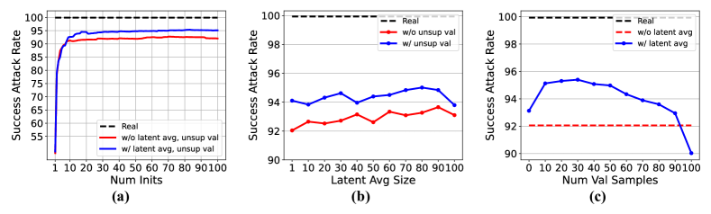
Figure 3: Results of variating hyperparameters (a) number of latents $n$, (b) size of latent averaging $t$, and (c) number of samples $k_{top}$ for unsupervised validation with LFW dataset.

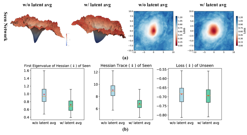
Figure 4: Loss surface landscape and contour line as heat map(a) of a single sample seen encoder with and without latent averaging applied. (b) Quantitative statistics are shown as box plot showing the first eigenvalue of hessian(left), trace of hessian(middle) for seen encoder and loss for unseen encoders measured with LFW samples.

Table 4: Averaged SAR of unseen encoders on LFW dataset. We compare multiple (denoted as 100$\times$100) with single (denoted as 1$\times$10k) latent optimization with periodic learning rate scheduler and the corresponding loss.

Target Encoder	Method	SAR@FAR			SAR
	($n\times iter$)	1e-4	1e-3	1e-2
	$1\times 10k$	9.44	22.15	30.08	26.22
FaceNet	$100\times 100$	61.79	79.75	91.2	86.3
	$1\times 10k$	59.01	82.72	89.76	85.92
MobFaceNet	$100\times 100$	69.1	94.5	99.01	97.62
	$1\times 10k$	22.8	29.7	34.87	32.29
ResNet50	$100\times 100$	75.76	92.69	97.51	95.81
	$1\times 10k$	55.56	72.68	78.99	76.13
ResNet100	$100\times 100$	80.35	97	99.31	98.91
	$1\times 10k$	49.31	66.36	71.32	69.48
Swin-S	$100\times 100$	76.07	97.32	99.43	99.07
	$1\times 10k$	54.86	68.34	75.52	71.62
VGGNet	$100\times 100$	75.15	89.14	96.37	92.94
Avg Cos Sim	$1\times 10k$	0.8842
at seen encoder	$100\times 100$	0.9813

Table 5: Comparing result with DiBiGAN[8] on each datasets. Experiments were done under the same white-box setting. We used 20 parallel latents to compare with [8].

Target Encoder	Method	Dataset
		LFW	CFP-FP	AgeDB-30
ResNet100	Real Face	99.96	97.1	98.4
	DiBiGAN	99.18	92.67	94.18
	Ours	99.85	96.59	98.33

Table 6: Quantitative face quality evaluation using 2 different types of FIQAs where higher values are better. Best results are highlighted with bold and second are underlined.

Metric	Real	NBNet	LatentMap	Genetic	GaussBlob	EigenFace	FaceTI	QEZOGE	Ours
SER-FIQ($\uparrow$)	0.774	0.612	0.661	0.664	0.005	0.519	0.748	0.701	0.746
CR-FIQA($\uparrow$)	2.191	1.756	2.139	2.181	0.747	1.723	2.198	2.262	2.107

4.5.3 Number of Latents and Optimization Steps

We compare optimizing 100 latents optimized 100 steps each (denoted as 100 $\times$ 100, without latent average and unsupervised validation) and a single latent optimized 10,000 steps with cyclical learning rate[13]. We train on LFW dataset where results are shown in Tab. 6. Our method outperforms with 95.13% in average SAR while serial optimization shows 60.28% resulting in a 34.85% performance gap. Despite the total steps of optimizations being identical, results highlight the importance of using multiple latents which prevents falling into poor local minima than interacting with complex learning rate scheduler as the difference of average cosine similarity shown in the last row of Tab. 6 is significant.

4.5.4 Latent Averaging and Loss Surface

In this section, we thoroughly analyze the effect of latent averaging. First of all, we visualize the loss surface of a sample in the seen encoder by adding perturbation in two random axes and using the method suggested in [16]. Additionally, we quantitatively compare the flatness of the optima point by measuring the first eigenvalue and trace of the Hessian matrix for every sample in LFW and the generalization by loss value on unseen encoders. Fig. 4a shows the shape of the loss surface where the z-axis is the loss value $1-sim(\cdot)$ where 1 is added to set the minimum loss value to 0. Applying latent average significantly improves the flatness visually as shown. In addition, the statistics of the first eigenvalue and trace of the Hessian matrix of latents with latent averaging have much lower values which indicate the curvature at the minima point is flatter while the loss value for unseen encoders is lower.

4.5.5 Unsupervised Validation with Pseudo Target

Unsupervised validation utilizes the feature space of a surrogate validation encoder to search for a better generalizing sample instead of only using the seen encoder. Hence, we compare the distance between the validation encoder’s top 1 and seen encoder’s top 1 against the ground truth feature in validation space (Fig. 5a) and examine whether this is relevant to generalizing to unseen encoder space (Fig. 5b). We also measure the distance between pseudo targets against ground truth in validation space to verify its efficacy as a target. We use LFW dataset and examine all 6 encoders as seen and unseen between each other as Tab. 1 with Swin-T as validation encoder and acquire the statistics of cosine distance.

As shown in Fig. 5a the pseudo target is closest to the ground truth feature from real images with average cosine distance $0.473$ followed by our unsupervised validation’s top 1 with $0.386$ and seen encoder’s top1 with $0.309$ in the validation space. According to this result, the pseudo target which is the closest to ground truth might be the best option, but unfortunately, the corresponding latent is inaccessible which is why we use the sample closest to the pseudo target. This aspect is connected to the unseen encoder space in Fig. 5b where our method shows average cosine distance $0.29$ higher than seen encoder’s top 1 $0.241$.

Furthermore, we examine results by changing the type of validation encoder. We use each encoder used in our work as a validation encoder and examine the performance improvement only for unseen cases where seen, unseen, and validation encoders do not overlap. Results shown in Fig. 5c presents that using any type of validation encoder improves performance and the improvement shows positive correlation with the general performance of validation encoder. More results are shown in Supp. 0.C Tab. 7.

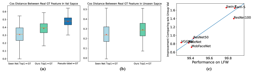
Figure 5: Statistics of cosine distance between seen encoder’s top 1, unsupervised validation’s top 1, and pseudo target against real image’s feature in validation feature space (a) and unseen encoder space (b) (pseudo target excluded since it only presents in validation space). (c) shows the correlation graph between the validation encoder’s performance and performance improvement.

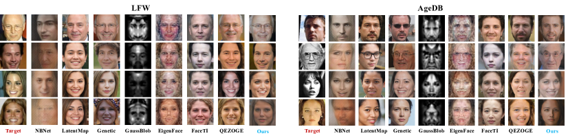
Figure 6: Sample images from baseline methods and ours on LFW and AgeDB.

4.5.6 Image Quality

We conduct qualitative and quantitative analyses of generated images. For quality evaluation, we compare a few samples from LFW and AgeDB in Fig. 6 and CFP-FP in Supp. 0.C Fig. 7. For quantitative evaluation, we adopt face-specific quality metrics SER-FIQ [30] and CR-FIQA [2]. NBNet, GaussBlob, and EigenFace show poor image quality visually with artifacts and quantitatively low image quality metrics. Meanwhile, despite the decent quality, LatentMap, Genetic, and FaceTI present wrong identities compared with the target images. On the other hand, QEZOGE and our method show decent image quality visually, quantitatively, and content-wise as shown in Tab. 6.

5 Conclusion

In this paper, we have presented a framework for face reconstruction transfer attacks. We devised our method inspired by out-of-distribution generalization to generalize our generated sample to unseen face encoders and propose ALSUV. ALSUV is instantiated by combining multiple latent optimization, latent averaging, and unsupervised validation with the pseudo target. We demonstrate that our approach surpasses previous methods in FRTA by showing high SAR and identification rate across various unseen face encoders. Our thorough analysis shows the effectiveness of our method inspired by OOD generalization. Furthermore, we hope our work alerts the security risk posed by FRTA, and emphasizes the awareness to mitigate potential threats.

Appendix 0.A Proof to Theorem

Theorem. Define $f_{z}$ by $f_{z}(\theta)=E_{\theta}(G(z))$, and let $D^{*}_{seen}=\{(\theta_{seen},v_{\theta_{seen}})\}$, $\mathcal{D}^{*}=\{\{(\theta,v_{\theta})\}:\theta\in\Theta\}$, and

$$l(f_{z}(\theta),v_{\theta})=-sim(f_{z}(\theta),v_{\theta}).$$ (10)

Then, $f_{z}$ is an MLP, and the FRTA algorithm $\mathcal{A}$ on $\Theta$ is an OOD generalization algorithm $\mathcal{A}^{*}$ on the domain $\mathcal{D}^{*}$ in the parameter space $\mathcal{Z}$.

Proof

(MLP) Since MLP is a composition of MLPs, it suffices to prove that a layer of $f_{z}$ is MLP. To this end, we show that the MLP $\sigma(\mathbf{W}\mathbf{x}+\mathbf{b})$ with input $\mathbf{x}$ and parameters $(\mathbf{W},\mathbf{b})$ is an MLP with input $(\mathbf{W},\mathbf{b})$ and parameters $\mathbf{x}$. Let $\mathbf{w}_{i}$ and $b_{i}$ denote the $i$-th row of $\mathbf{W}$ and $\mathbf{b}$, respectively, for $i=1,\dots,r$ where $r$ is the row dimension of $\mathbf{W}$. Observe,

$$\sigma(\mathbf{W}\mathbf{x}+\mathbf{b})=\sigma\left(diag(\mathbf{x})\mathbf{w}_{i}+b_{i}\mathbf{1}\right)$$ (11)

where $diag(\mathbf{x})$ is the diagonal matrix whose diagonal elements are $x_{i}$, and $\mathbf{1}$ is a vector whose all entries are $1$. Both

$$f_{1}((\mathbf{W},\mathbf{b});\mathbf{x})=diag(\mathbf{x})\mathbf{w}_{i}$$ (12)

and

$$f_{2}((\mathbf{W},\mathbf{b});\mathbf{x})=b_{i}\mathbf{1}$$ (13)

are MLPs with input $(\mathbf{W},\mathbf{b})$ and parameters $\mathbf{x}$, hence their sum and activattion are also MLPs with the same aspect, completing the proof.

(Equivalence) We show the equivalence between FRTA and OOD generalization. To see this, first define

$$L(z;D^{*}):=\frac{1}{|D^{*}|}\sum_{(\theta,v_{\theta})\in D^{*}}l(f_{z}(\theta),v_{\theta})$$ (14)

Then, observe that

$$\mathcal{A}^{*}(D^{*}_{seen}) :=\min_{z}\max_{D^{*}\in\mathcal{D}^{*}}L(z;D^{*})$$

$$=\min_{z}\max_{D^{*}\in\mathcal{D}^{*}}l(f_{z}(\theta),v_{\theta})$$

$$=\min_{z}\max_{D^{*}\in\mathcal{D}^{*}}-sim(f_{z}(\theta),v_{\theta})$$

$$=\max_{z}\min_{\theta\in\Theta}sim(f_{z}(\theta),v_{\theta})$$

$$=:\mathcal{A}(\theta_{seen})$$

where the second and fourth equations hold due to $D^{*}=\{(\theta,v_{\theta})\}$, completing the proof.

Appendix 0.B Supplementary to Method

0.B.1 Algorithm of the full method

The full algorithm of our method is given in Algorithm. 1. In this algorithm, $[z_{i}]_{i=1}^{n}$ is the vector concatenation of the vectors $z_{i}$, which is to parallelize the update of $z_{i}$’s.

Algorithm 1 The algorithm of our method

1:$\{z_{i}\}_{i=1}^{n},E_{\theta_{seen}},G,v_{seen},T,T_{0},E_{\theta_{val}},k_{top}$

2:$z^{*}$

3:# Optimizing Multiple Latents

4:Initialize $z_{i}^{(0)}=z_{i}$ for $i=1,\dots,n$

5:for $t=1,\dots,T$ do

6:     $[z_{i}^{(t)}]_{i=1}^{n}\leftarrow[z_{i}^{(t-1)}]_{i=1}^{n}+\lambda\nabla_{[z_{i}]_{i=1}^{n}}\sum_{i=1}^{n}\operatorname{sim}(E_{\theta_{seen}}(G(z_{i})),v_{seen})\mid_{[z_{i}]_{i=1}^{n}=[z_{i}^{(t-1)}]_{i=1}^{n}}$ $\triangleright$ by Adam optimizer

7:end for

8:# Latent Averaging

9:$\overline{z}_{i}\leftarrow\frac{1}{T_{0}}\sum_{t=T-T_{0}}^{T}z_{i}^{(t)}$

10:# Unsupervised Validation with Pseudo Target

11:Order the index $i$ of $\overline{z}_{i}$ such that $\operatorname{sim}(E_{\theta_{seen}}(G(\overline{z}_{i+1})),v_{seen})\leq\operatorname{sim}(E_{\theta_{seen}}(G(\overline{z}_{i})),v_{seen})$

12:$m=\frac{1}{k_{top}}\sum_{i=1}^{k_{top}}E_{\theta_{val}}(G(\overline{z}_{i}))$ $\triangleright$ pseudo target to the validation encoder embedding of real image

13:$z^{*}=\underset{z\in\{\overline{z}_{i}\}_{i=1}^{k_{top}}}{\arg\max}\operatorname{sim}(E_{\theta_{val}}(G(z)),m)$

Appendix 0.C Supplementary Results

Fig. 7 shows the result of reconstructed images from CFP-FP dataset of each baselines, our method and ground truth images.

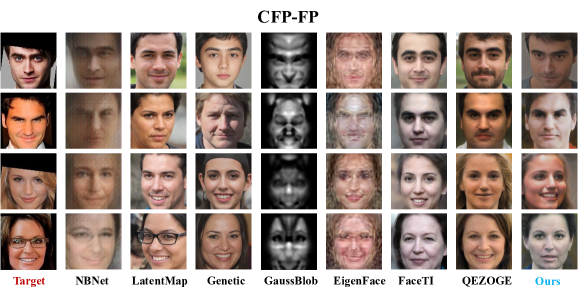
Figure 7: Sample images of previous methods and ours from CFP-FP dataset.

Tab. 7 ablates pseudo target of unsupervised validation by using different types of target for searching the top 1 reconstructed sample. We compare SAR of 3 different cases: using the seen feature vector as target in the seen encoder space, using validation encoder and the pseudo target in the validation encoder space, and using the unseen encoder and the feature vector from real image in the unseen encoder space where the last works as a reference to upper bound performance.

Table 7: SAR comparison by using different targets when choosing top 1 sample. We compare using seen feature vector in seen encoder space(equivalent to not using unsupervised validation) denoted as Seen Feature, our pseudo target in validation encoder space denoted as Pseudo Target, and feature vector of real image in unseen encoder space which works as reference to upper bound which is denoted as Upper Bound. Unsupervised validation results are highlighted with gray and best performances (except upper bound) are highlighted with bold.

Dataset		LFW
Target Encoder	Method	FaceNet	MobFace	ResNet50	ResNet100	Swin-S	VGGNet	Unseen AVG
	Seen Feature	99.87	55.81	97.44	81.53	79.84	99.39	82.8
	Pseudo Target	99.83	65.15	97.51	86.79	83.32	99.22	86.4
FaceNet	Upper bound	99.87	91.51	99.19	97.34	95.25	99.66	96.59
	Seen Feature	95.72	99.87	96.6	96.73	99.09	97.88	97.2
	Pseudo Target	96.76	99.83	97.3	96.83	99.16	98.05	97.62
MobFace	Upper bound	98.75	99.87	99.26	99.53	99.6	99.19	99.27
	Seen Feature	98.99	77.15	99.76	96.49	95.38	99.73	93.55
	Pseudo Target	99.12	85.24	99.8	97.44	97.61	99.63	95.81
ResNet50	Upper bound	99.49	95.96	99.76	99.63	99.36	99.63	98.81
	Seen Feature	99.39	93.93	99.6	99.93	99.87	99.53	98.46
	Pseudo Target	99.36	96.16	99.56	99.93	99.93	99.56	98.91
ResNet100	Upper bound	99.53	99.36	99.8	99.93	99.93	99.7	99.66
	Seen Feature	98.42	98.18	99.12	99.73	99.93	99.33	98.96
	Pseudo Target	98.08	99.02	99.02	99.87	99.93	99.36	99.07
Swin-S	Upper bound	99.36	99.56	99.56	99.93	99.93	99.66	99.61
	Seen Feature	99.26	66.33	99.49	93.46	89.15	99.76	89.54
	Pseudo Target	99.29	77.45	99.49	94.57	93.9	99.8	92.94
VGGNet	Upper bound	99.6	97.17	99.73	99.09	98.85	99.8	98.89

Appendix 0.D Supplementary Setup

Tab. 8 shows the configuration of each face encoders used in all experiments.

Table 8: Training configuration of the face encoders used in our experiments. For FaceNet, we use the pre-trained model from facenet-pytorch library. For MobileFaceNet and Swin-S, we use pre-trained models from [32]. For ResNet100, we use the model from the official ArcFace github. ResNet50 and VGG19 models were trained by ourselves. Finally, we use Swin-T for validation encoder.

Backbone	Classification Head	Dataset
FaceNet[26]	Triplet Loss	CASIA-WebFace[34]
MobileFaceNet[4]	Additive Margin Softmax[33]	MS-CELEB-1M[10]
ResNet50[11]	CosFace[31]	MS-CELEB-1M
ResNet100	ArcFace[5]	MS-CELEB-1M-v3
SwinTransformer-S[17]	Additive Margin Softmax	MS-CELEB-1M
VGGNet[29]	CosFace	MS-CELEB-1M

References

- [1] Berthelot, D., Carlini, N., Goodfellow, I., Papernot, N., Oliver, A., Raffel, C.A.: Mixmatch: A holistic approach to semi-supervised learning. Advances in neural information processing systems 32 (2019)
- [2] Boutros, F., Fang, M., Klemt, M., Fu, B., Damer, N.: Cr-fiqa: face image quality assessment by learning sample relative classifiability. In: Proceedings of the IEEE/CVF Conference on Computer Vision and Pattern Recognition. pp. 5836–5845 (2023)
- [3] Cha, J., Chun, S., Lee, K., Cho, H.C., Park, S., Lee, Y., Park, S.: Swad: Domain generalization by seeking flat minima. Advances in Neural Information Processing Systems 34, 22405–22418 (2021)
- [4] Chen, S., Liu, Y., Gao, X., Han, Z.: Mobilefacenets: Efficient cnns for accurate real-time face verification on mobile devices. In: Biometric Recognition: 13th Chinese Conference, CCBR 2018, Urumqi, China, August 11-12, 2018, Proceedings 13. pp. 428–438. Springer (2018)
- [5] Deng, J., Guo, J., Xue, N., Zafeiriou, S.: Arcface: Additive angular margin loss for deep face recognition. In: Proceedings of the IEEE/CVF conference on computer vision and pattern recognition. pp. 4690–4699 (2019)
- [6] Dong, X., Jin, Z., Guo, Z., Teoh, A.B.J.: Towards generating high definition face images from deep templates. In: 2021 International Conference of the Biometrics Special Interest Group (BIOSIG). pp. 1–11. IEEE (2021)
- [7] Dong, X., Miao, Z., Ma, L., Shen, J., Jin, Z., Guo, Z., Teoh, A.B.J.: Reconstruct face from features based on genetic algorithm using gan generator as a distribution constraint. Computers & Security 125, 103026 (2023)
- [8] Duong, C.N., Truong, T.D., Luu, K., Quach, K.G., Bui, H., Roy, K.: Vec2face: Unveil human faces from their blackbox features in face recognition. In: Proceedings of the IEEE/CVF Conference on Computer Vision and Pattern Recognition. pp. 6132–6141 (2020)
- [9] Garipov, T., Izmailov, P., Podoprikhin, D., Vetrov, D.P., Wilson, A.G.: Loss surfaces, mode connectivity, and fast ensembling of dnns. Advances in neural information processing systems 31 (2018)
- [10] Guo, Y., Zhang, L., Hu, Y., He, X., Gao, J.: Ms-celeb-1m: A dataset and benchmark for large-scale face recognition. In: ECCV (2016)
- [11] He, K., Zhang, X., Ren, S., Sun, J.: Deep residual learning for image recognition. In: Proceedings of the IEEE conference on computer vision and pattern recognition. pp. 770–778 (2016)
- [12] Hu, Z., Yang, Z., Hu, X., Nevatia, R.: Simple: Similar pseudo label exploitation for semi-supervised classification. In: Proceedings of the IEEE/CVF Conference on Computer Vision and Pattern Recognition. pp. 15099–15108 (2021)
- [13] Izmailov, P., Podoprikhin, D., Garipov, T., Vetrov, D., Wilson, A.G.: Averaging weights leads to wider optima and better generalization. arXiv preprint arXiv:1803.05407 (2018)
- [14] Karras, T., Laine, S., Aila, T.: A style-based generator architecture for generative adversarial networks. In: Proceedings of the IEEE/CVF conference on computer vision and pattern recognition. pp. 4401–4410 (2019)
- [15] Kingma, D.P., Ba, J.: Adam: A method for stochastic optimization. arXiv preprint arXiv:1412.6980 (2014)
- [16] Li, H., Xu, Z., Taylor, G., Studer, C., Goldstein, T.: Visualizing the loss landscape of neural nets. Advances in neural information processing systems 31 (2018)
- [17] Liu, Z., Lin, Y., Cao, Y., Hu, H., Wei, Y., Zhang, Z., Lin, S., Guo, B.: Swin transformer: Hierarchical vision transformer using shifted windows. In: Proceedings of the IEEE/CVF international conference on computer vision. pp. 10012–10022 (2021)
- [18] Mai, G., Cao, K., Yuen, P.C., Jain, A.K.: On the reconstruction of face images from deep face templates. IEEE transactions on pattern analysis and machine intelligence 41(5), 1188–1202 (2018)
- [19] Park, H., Park, J., Dong, X., Teoh, A.B.J.: Towards query efficient and generalizable black-box face reconstruction attack. In: 2023 IEEE International Conference on Image Processing (ICIP). pp. 1060–1064. IEEE (2023)
- [20] Paszke, A., Gross, S., Massa, F., Lerer, A., Bradbury, J., Chanan, G., Killeen, T., Lin, Z., Gimelshein, N., Antiga, L., et al.: Pytorch: An imperative style, high-performance deep learning library. Advances in neural information processing systems 32 (2019)
- [21] Petzka, H., Kamp, M., Adilova, L., Sminchisescu, C., Boley, M.: Relative flatness and generalization. Advances in neural information processing systems 34, 18420–18432 (2021)
- [22] Rame, A., Kirchmeyer, M., Rahier, T., Rakotomamonjy, A., Gallinari, P., Cord, M.: Diverse weight averaging for out-of-distribution generalization. Advances in Neural Information Processing Systems 35, 10821–10836 (2022)
- [23] Razzhigaev, A., Kireev, K., Kaziakhmedov, E., Tursynbek, N., Petiushko, A.: Black-box face recovery from identity features. In: Computer Vision–ECCV 2020 Workshops: Glasgow, UK, August 23–28, 2020, Proceedings, Part V 16. pp. 462–475. Springer (2020)
- [24] Razzhigaev, A., Kireev, K., Udovichenko, I., Petiushko, A.: Darker than black-box: Face reconstruction from similarity queries. arXiv preprint arXiv:2106.14290 (2021)
- [25] Saito, K., Watanabe, K., Ushiku, Y., Harada, T.: Maximum classifier discrepancy for unsupervised domain adaptation. In: Proceedings of the IEEE conference on computer vision and pattern recognition. pp. 3723–3732 (2018)
- [26] Schroff, F., Kalenichenko, D., Philbin, J.: Facenet: A unified embedding for face recognition and clustering. In: Proceedings of the IEEE conference on computer vision and pattern recognition. pp. 815–823 (2015)
- [27] Shahreza, H.O., Marcel, S.: Face reconstruction from facial templates by learning latent space of a generator network. In: Thirty-seventh Conference on Neural Information Processing Systems (2023), https://openreview.net/forum?id=hI6EPhq70A
- [28] Shin, I., Woo, S., Pan, F., Kweon, I.S.: Two-phase pseudo label densification for self-training based domain adaptation. In: Computer Vision–ECCV 2020: 16th European Conference, Glasgow, UK, August 23–28, 2020, Proceedings, Part XIII 16. pp. 532–548. Springer (2020)
- [29] Simonyan, K., Zisserman, A.: Very deep convolutional networks for large-scale image recognition. arXiv preprint arXiv:1409.1556 (2014)
- [30] Terhorst, P., Kolf, J.N., Damer, N., Kirchbuchner, F., Kuijper, A.: Ser-fiq: Unsupervised estimation of face image quality based on stochastic embedding robustness. In: Proceedings of the IEEE/CVF conference on computer vision and pattern recognition. pp. 5651–5660 (2020)
- [31] Wang, H., Wang, Y., Zhou, Z., Ji, X., Gong, D., Zhou, J., Li, Z., Liu, W.: Cosface: Large margin cosine loss for deep face recognition. In: Proceedings of the IEEE conference on computer vision and pattern recognition. pp. 5265–5274 (2018)
- [32] Wang, J., Liu, Y., Hu, Y., Shi, H., Mei, T.: Facex-zoo: A pytorh toolbox for face recognition (2021)
- [33] Wang, X., Zhang, S., Wang, S., Fu, T., Shi, H., Mei, T.: Mis-classified vector guided softmax loss for face recognition. In: Proceedings of the AAAI Conference on Artificial Intelligence. vol. 34, pp. 12241–12248 (2020)
- [34] Yi, D., Lei, Z., Liao, S., Li, S.Z.: Learning face representation from scratch. arXiv preprint arXiv:1411.7923 (2014)
- [35] Zhang, H., Cisse, M., Dauphin, Y.N., Lopez-Paz, D.: mixup: Beyond empirical risk minimization. arXiv preprint arXiv:1710.09412 (2017)
- [36] Zou, Y., Yu, Z., Kumar, B., Wang, J.: Unsupervised domain adaptation for semantic segmentation via class-balanced self-training. In: Proceedings of the European conference on computer vision (ECCV). pp. 289–305 (2018)
- [37] Zou, Y., Yu, Z., Liu, X., Kumar, B., Wang, J.: Confidence regularized self-training. In: Proceedings of the IEEE/CVF international conference on computer vision. pp. 5982–5991 (2019)