Consistency Flow Matching:
Defining Straight Flows with Velocity Consistency

Abstract

Flow matching (FM) is a general framework for defining probability paths via Ordinary Differential Equations (ODEs) to transform between noise and data samples. Recent approaches attempt to straighten these flow trajectories to generate high-quality samples with fewer function evaluations, typically through iterative rectification methods or optimal transport solutions. In this paper, we introduce Consistency Flow Matching (Consistency-FM), a novel FM method that explicitly enforces self-consistency in the velocity field. Consistency-FM directly defines straight flows starting from different times to the same endpoint, imposing constraints on their velocity values. Additionally, we propose a multi-segment training approach for Consistency-FM to enhance expressiveness, achieving a better trade-off between sampling quality and speed. Experiments demonstrate that our Consistency-FM significantly improves training efficiency by converging 4.4x faster than consistency models and 1.7x faster than rectified flow models while achieving better generation quality. Our code is available at https://github.com/YangLing0818/consistency_flow_matching

1 Introduction

In recent years, deep generative models have provide an attractive family of paradigms that can produce high-quality samples by modeling a data distribution, achieving promising results in many generative scenarios, such as image generation [1, 2, 3, 4]. As a general and deterministic framework, Continuous Normalizing Flows (CNFs) [5] are capable of modeling arbitrary probability paths, specifically including the probability paths represented by diffusion processes [6]. To scale up the training of CNFs, many works propose efficient simulation-free approaches [7, 8, 9] by parameterizing a vector field which flows from noise samples to data samples. Lipman et al. (2022) [7] proposes Flow Matching (FM) to train CNFs based on constructing explicit conditional probability paths between the noise distribution and each data sample. Taking inspiration from denoising score matching [10], FM further shows that a per-example training objective can provide equivalent gradients without requiring explicit knowledge of the intractable target vector field, thus incorporating existing diffusion paths as special instances.

Straightness is one particularly-desired property of the trajectory induced by FM [9, 11, 12, 13], because the straight path are not only the shortest path between two end points, but also can be exactly simulated without time discretization. To learn straight line paths which transport distribution $\pi_{0}$ to $\pi_{1}$, Liu et al. (2022) [9] learn a rectified flow from data by turning an arbitrary coupling of $\pi_{0}$ and $\pi_{1}$ to a new deterministic coupling, and iteratively train new rectified flows with the data simulated from the previously obtained rectified flow. Some works resort to optimizing with an optimal transport plan by considering non-independent couplings of k-sample empirical distributions [14, 13]. For example, OT-CFM [13] attempts to approximate dynamic OT, creating simpler flows that are more stable to train and lead to faster inference.

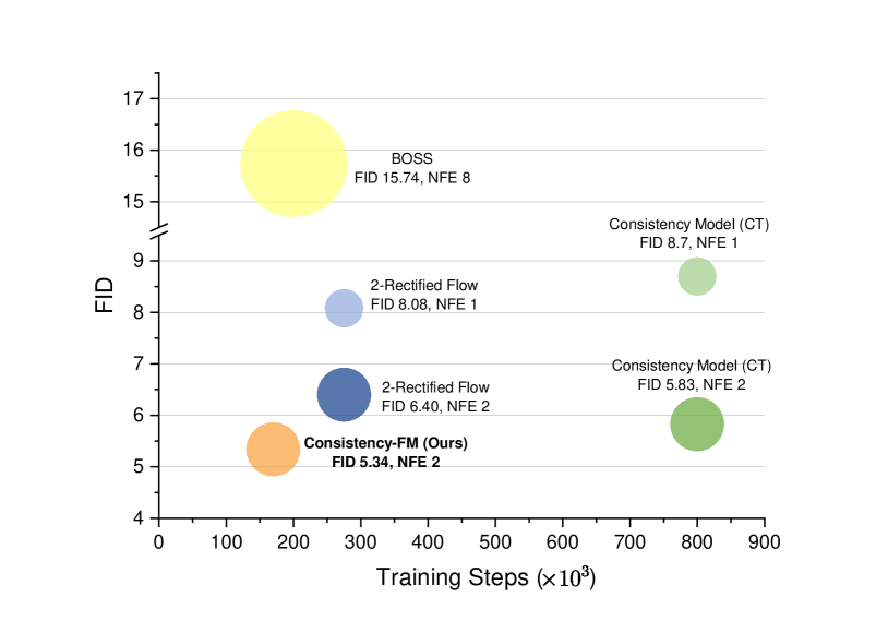
Figure 1: Comparison on CIFAR-10 dataset regarding the trade-off between generation quality and training efficiency. Our Consistency-FM demonstrates the best trade-off compared to consistency models [15] and rectified flow models [9, 16], converging 4.4 times faster than consistency models and 1.7 times faster than rectified flow models while achieving better generation quality

However, despite their impressive generation quality, they still lack an effective trade-off between sampling quality and computational cost in straightening flows. To be more specifically, iterative rectification would suffer from accumulation error, and approximating an optimal transport plan in each training batch is computationally expensive. Therefore, a question naturally arises, can one learn an effective ODE model that maximally straightens the trajectories of probability flows without increasing training complexity?

In this work, we propose a new fundamental FM method, namely Consistency Flow Matching (Consistency-FM), to straighten the flows by explicitly enforcing self-consistency property in the velocity field. More specifically, Consistency-FM directly defines straight flows that start from different times to the same endpoint, and further constrains on their velocity values. To enhance the model expressiveness and enable better transporting between complex distributions, we resort to training Consistency-FM in a multi-segment approach, which constructs a piece-wise linear trajectory. Moreover, this flexible time-to-time jump allows Consistency-FM to perform distillation on pre-trained FM models for better trade-off between sampling speed and quality.

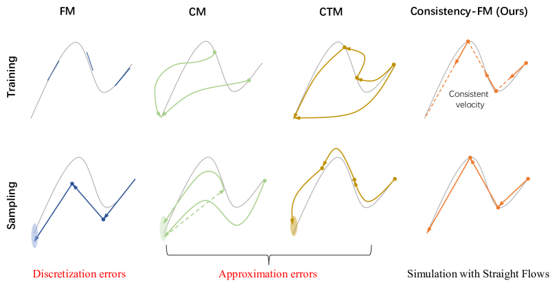
Figure 2: Training and sampling comparisons between flow matching (FM) [7], consistency model (CM) [15] and consistency trajectory model (CTM) [17] and our Consistency-FM. While previous methods can cause discretization errors or approximation errors, Consistency-FM mitigates these issues by defining straight flows in simulation.

Comparison with Consistency Models

Consistency Models (CMs) [15] learn a set of consistency functions that directly map noise to data. While CMs can generate sample with one NFE, but they fail to provide a satisfying trade-off between generation quality and computational cost [17]. Moreover, enforcing consistency property at arbitrary points is redundant and potentially slows down the training process. In contrast, our Consistency-FM enforces the consistency property over the space of velocity field instead of sample space, which can be viewed as a high-level regularization for straightening ODE trajectory. While CMs is able to learn consistency functions in a general form, Consistency-FM parameterizes the consistency functions as straight flows, which enables faster training convergence without the need for approximating the entire probability path.

Main Contributions

We summarize our contributions as follows: (i) We propose a new fundamental class of FM models that explicitly enforces the self-consistency in the space of velocity field instead of sample space. (ii) We conduct sufficient theoretical analysis for our proposed Consistency-FM, and enhance its expressiveness with multi-segment optimization. (iii) Preliminary experiments on three classical image datasets demonstrate the superior generation quality and training efficiency of our Consistency-FM (e.g., 4.4 times and 1.7 times faster than consistency model and rectified flow).

2 Related Work and Discussions

Flow Matching for Generative Modeling

Flow Matching (FM) aims to (implicitly) learn a vector field $\{v_{t}\}_{t\in[0,1]}$, which generates an ODE that admits to the desired probability path $\{p_{t}\}_{t\in[0,1]}$ [7]. The training of FM does not require any computational challenging simulation, as it directly estimate the vector field using a regression objective which can be efficiently estimated [7]. By the construction of FM, it allows general trajectory of ODE and probability path, thus many effort have been dedicated to design better trajectory with certain properties[14, 13, 18, 19, 20]. One particularly desired property is the straightness of the trajectory, as a straight trajectory can be efficiently simulated with few steps of Euler integration. Concurrent works Multisample FM [14] and Minibatch OT [13] propose to generalize the independent coupling of data distribution $p_{0}(x_{0})$ and prior distribution $p_{1}(x_{1})$ to optimal transport coupling plan $\pi(x_{0},x_{1})$. Under the optimal transport plan, the learned trajectory of ODE will tend to be straight. However, their methods require constructing the approximated optimal transport plan in each training batch, which is computationally prohibitive.

Rectified Flow [9, 11] can be viewed as a FM with specific trajectory. Rectified Flow proposes to rewire and straighten the trajectory by iterative distillation, which requires multiple round of training and may suffer from accumulation error. A recent work, Optimal FM [12] proposes to directly learn the optimal transport map from $p_{1}$ to $p_{0}$ and use it to calculate the vector field and straight trajectory. However, computing the optimal transport map in high dimension is a challenging task [21], and Optimal FM [12] only provides experiments on toy datasets. In this paper, we propose to straighten the trajectory in a more flexible and effective approach by enforcing the self-consistency property in the velocity field.

Learning Efficient Generative Models

GANs [22, 23], VAEs [24], Diffusion Models [25, 26, 1] and Normalizing Flows [27, 28] have been four classical deep generative models. Among them, GANs and VAEs are efficient one-step models. However, GANs usually suffer from the training instability and mode collapse issues, and VAEs may struggle to generate high-quality examples. Therefore, recent works begin to utilize diffusion models and continuous normalizing flows [5] for better training stability and high-fidelity generation, which are based on a sequence of expressive transformations for generative sampling.

To achieve a better trade-off between sampling quality and speed, many efforts have been made to accelerate diffusion models, either by modifying the diffusion process [26, 29, 30, 31, 4], with an efficient ODE solver [32, 33, 34], or performing distillation between pre-trained diffusion models and their more efficient versions (e.g., with less sampling steps) [35, 9, 36, 37]. However, most distillation methods require multiple training rounds and are susceptible to accumulation errors. Recent Consistency Models [15, 38] distill the entire sampling process of diffusion model into one-step generation, while maintaining good sample quality. Consistency Trajectory Models (CTMs)[17] further mitigate the issues about the accumulated errors in multi-step sampling. However, these method must learn to integrate the full ODE integral, which are difficult to learn when it jumps between modes of the target distribution. In this paper, we propose a new concept of velocity consistency with defined straight probability flows, achieving most competitive results on both one- and multi-step generation.

3 Consistency Flow Matching

3.1 Preliminaries on Flow Matching

Let $\mathcal{R}^{d}$ denote the data space with data point $x_{0}\in\mathcal{R}^{d}$, FMs aim to the learn a vector field $v_{\theta}(t,x):[0,1]\times\mathcal{R}^{d}\xrightarrow{}\mathcal{R}^{d}$, such that the solution of the following ODE can transport noise $x_{0}~{}\sim p_{0}$ to data $x_{1}~{}\sim p_{1}$:

$$\left\{\begin{aligned} &\frac{d\gamma_{x}(t)}{dt}=v_{\theta}(t,\gamma_{x}(t)),\\ &\gamma_{x}(0)=x\end{aligned}\right.$$ (1)

The solution of Eq. 1 is denoted by $\gamma_{x}(\cdot)$, which is also called a flow, describing the trajectory of the ODE from starting point $x$. Given the ground truth vector field $u(t,x)$ that generates probability path $p_{t}$ under the two marginal constraints that $p_{t=0}=p_{0}$ and $p_{t=1}=p_{1}$, FMs seek to optimize the simple regression objective

$$E_{t,p_{t}}||v_{\theta}(t,x_{t})-u(t,x_{t})||_{2}^{2}$$ (2)

However, it is computational intractable to find such $u$, since $u$ and $p_{t}$ are governed by the following continuity equation [39]:

$$\partial_{t}p_{t}(x)=-\nabla\cdot(u(t,x)p_{t}(x))$$ (3)

Instead of directly optimizing Eq. 2, Conditional Flow Matching [7] regress $v_{\theta}(t,x)$ on the conditional vector filed $u(t,x_{t}|x_{1})$ and probability path $p_{t}(x_{t}|x_{1})$ :

$$E_{t,q(x_{1})}E_{p_{t}(x_{t}|x_{1})}||v_{\theta}(t,x_{t})-u(t,x_{t}|x_{1})||_{2}^{2}$$ (4)

Two objectives Eq. 2 and Eq. 4 share the same gradient with respect to $\theta$, while Eq. 4 can be efficiently estimated as long as the conditional pair $u(t,x_{t}|x_{1}),p_{t}(x_{t}|x_{1})$ is tractable. Note that recovering the marginal vector field and probability path from the conditioned one remains a complex challenge [7].

3.2 Defining Straight Flows with Consistent Velocity

Motivation

Recent FM methods for learning straight flows typically necessitate the approximation the probability path $p_{t}$ and its marginal distributions $p_{0}$ and $p_{1}$ [9, 11, 14, 40] , which are computational intensive and introduce additional approximation error. To address these challenges, we introduce Consistency-FM, a general method to efficiently learn straight flows without the need for approximating the entire probability path.

A straightforward approach to learn straight flows is to identify a consistent ground truth vector field and then use objective in Eq. 2 for training. The definition of consistent velocity is $v(t,\gamma_{x}(t))=v(0,x)$, indicating the velocity along the solution of Eq. 1 remains constant. However, due to the intractability of original data distribution, it is also intractable to find such a vector field, or to design a conditional vector field such that the corresponding marginal velocity is consistent [7, 14].

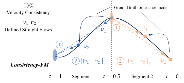
Figure 3: Ilustration of training our consistency-FM.

Instead of directly regressing on the ground truth vector field, Consistency-FM directly defines straight flows with consistent velocity that start from different times to the same endpoint. Specifically, we have the following lemma (prove in Appendix A.1):

Lemma 1.

Assuming the vector field is Lipschitz with respect to $x$ and uniform in $t$, and are differentiable in both input, then these two conditions are equivalent:

$$\textit{Condition 1.}\quad v(t,\gamma_{x}(t))=v(s,\gamma_{x}(s)),\quad\forall t,s\in[0,1]$$ (5)

$$\textit{Condition 2.}\quad\gamma_{x}(t)+(1-t)*v(t,\gamma_{x}(t))=\gamma_{x}(s)+(1-s)*v(s,\gamma_{x}(s)),\quad\forall t,s\in[0,1],$$

where $\gamma_{x}(t)$ represents the solution of Eq. 1 at time $t$. Condition 2 specifies that starting from an arbitrary time $t$ with data point $\gamma_{x}(t)$, and moving in the direction of current velocity for a duration of $1-t$, the resulting data will be consistent and independent with respect to $t$.

Velocity Consistency Loss

While Condition 1 directly constraints the vector field to be consistent, learning vector fields that only satisfy Condition 1 may lead to trivial solutions. On the other hand, Condition 2 ensures the consistency of the vector field from a trajectory viewpoint, offering a way to directly define straight flows. Motivated by this, Consistency-FM learns a consistency vector field to satisfy both conditions:

$$\mathcal{L}_{\theta}=E_{t\sim\mathcal{U}}E_{x_{t},x_{t+\Delta t}}||f_{\theta}(t,x_{t})-f_{\theta^{-}}(t+\Delta t,x_{t+\Delta t})||_{2}^{2}+\alpha||v_{\theta}(t,x_{t})-v_{\theta^{-}}(t+\Delta t,x_{t+\Delta t})||_{2}^{2},$$ (6)

$$f_{\theta}(t,x_{t})=x_{t}+(1-t)*v_{\theta}(t,x_{t}),$$

where $\mathcal{U}$ is the uniform distribution on $[0,1-\Delta t]$, $\alpha$ is a positive scalar, $\Delta t$ denotes a time interval which is a small and positive scalar. $\theta^{-}$ denotes the running average of past values of $\theta$ using exponential moving average (EMA), $x_{t}$ and $x_{t+\Delta t}$ follows a pre-defined distribution which can be efficiently sampled, for example, VP-SDE [1] or OT path [7]. Note that by setting $t=1$, Condition 2 implies that $\gamma_{x}(t)+(1-t)*v(t,\gamma_{x}(t))=\gamma_{x}(1)\sim p_{1}$, and thus training with $\mathcal{L}_{\theta}$ can not only regularize the velocity but also learn the data distribution. Furthermore, if Condition 2 is met, then the straight flows $\gamma_{x}(t)+(1-t)*v(t,\gamma_{x}(t))$ can directly predict $x_{1}$ from each time point $t$ [15].

Below we provide a theoretical justification for the objective based on asymptotic analysis (proof in Appendix A.3).

Theorem 1.

Consider no exponential moving average, i.e., $\theta^{-}=\theta$. Assume there exists ground truth velocity field $u_{t}$ that generates $p_{t}$ and satisfies the continuity Eq. 3. Furthermore we assume $v_{\theta}$ is bounded and twice continuously differentiable with bounded first and second derivatives, the ground truth velocity $u_{t}$ is bounded. Then we have:

$$E||f_{\theta}(t,x_{t})-f_{\theta}(t+\Delta t,x_{t+\Delta t})||_{2}^{2}=(\Delta t)^{2}E||v_{\theta}(t,x_{t})-u(t,x_{t})-(1-t)(\partial_{t}v_{\theta}+u\cdot\nabla_{x}v_{\theta})||_{2}^{2}+o((\Delta t)^{2})$$ (7)

Remark 1. The objective in Eq. 7,

$$E||v_{\theta}(t,x_{t})-u(t,x_{t})-(1-t)(\partial_{t}v_{\theta}+u\cdot\nabla_{x}v_{\theta})||_{2}^{2},$$

can be seen as striking a balance between exact velocity estimation and adhering to consistent velocity constraints. On the one hand, the objective aims to minimize the discrepancy between learned and ground truth velocity $v_{\theta}(t,x_{t})-u(t,x_{t})$, aligning with the goal of FM-based methods [7]. On the other hand, it also considers the consistency of the velocity. By Lemma 2 in the Appendix, $\partial_{t}v_{\theta}+u\cdot\nabla_{x}v_{\theta}$ serves as a constraint for velocity consistency, which measures the changes of the velocity after taking a infinitesimal step along the direction of ground truth velocity. Given the ground truth velocity may not be consistent, this objective provides a trade-off between the sampling quality and computational cost with straight flow.

3.3 Multi-Segment Consistency-FM

To enhance the expressiveness of Consistency-FM for transporting distributions in general probability path, we introduce Multi-Segment Consistency-FM. This approach relaxes the requirement for consistent velocity throughout the flow, allowing for more flexible adaptations to diverse distribution characteristics. Multi-Segment Consistency-FM divides the time interval into equal segments, learning a consistent vector field $v_{\theta}^{i}$ within each segment. After recombining these segments, it constructs a piece-wise linear trajectory to transport noise to data distribution. Specifically, given a segment number $K$, the time interval $[0,1]$ is divided with $[0,1]=\Sigma_{i=0}^{K-1}[i/K,(i+1)/K]$. Then the training objective is defined as

$$\mathcal{L}_{\theta}=E_{t\sim\mathcal{U}^{i}}\lambda^{i}E_{x_{t},x_{t+\Delta t}}||f_{\theta}^{i}(t,x_{t})-f_{\theta^{-}}^{i}(t+\Delta t,x_{t+\Delta t})||_{2}^{2}+\alpha||v_{\theta}^{i}(t,x_{t})-v_{\theta^{-}}^{i}(t+\Delta t,x_{t+\Delta t})||_{2}^{2},$$ (8)

$$f_{\theta}^{i}(t,x_{t})=x_{t}+((i+1)/k-t)*v_{\theta}^{i}(t,x_{t}),$$

where $i$ denotes the $i^{th}$ segment, $\mathcal{U}^{i}$ is the uniform distribution on $[i/K,(i+1)/K-\Delta t]$, $x_{t},x_{t+\Delta t}$ follow a pre-defined distribution, $\Delta t$ is a small and positive constant . $v_{\theta}^{i}(t,x_{t})$ are the flow and the consistent vector field in segment $i$, respectively. $\lambda^{i}$ is a positive weighting scalar for different segment, as vector field in the middle of $[0,1]$ is more difficult to train [41].

Below we provide a theoretical justification for multi-segment training. First, we analysis the optimal solution for objective Eq. 8 and provide a explicit formula for the estimation error in Multi-Segment Consistency-FM (proof in Appendix Section A.4):

Theorem 2.

Consider training consistency-FM on segment $i$ which is defined in time interval $[S,T]$. Assume there exists ground truth velocity field $u_{t}$ that generates $p_{t}$ and satisfies the continuity equation Eq. 3, let $v^{*}(t,x)$ denote the oracle consistent velocity such that

$$x_{T}=x_{t}+(T-t)v^{*}(t,x_{t}).$$ (9)

Then the learned $v_{\theta}^{i}(t,x_{t})$ that minimize Eq. 8 in segment $i$ at time $t\in[S,T-\Delta t]$ has the following error:

$$v_{\theta}^{i}(t,x_{t})-v^{*}(t,x_{t})= \frac{\alpha}{(T-t)^{2}+\alpha}(v^{*}(t+\Delta t,x_{t+\Delta t})-v^{*}(t,x_{t}))$$ (10)

$$+\frac{(T-t-\Delta t)(T-t)+\alpha}{(T-t)^{2}+\alpha}(v_{\theta}^{i}(t+\Delta t,x_{t+\Delta t})-v^{*}(t+\Delta t,x_{t+\Delta t}))$$

Remark 2. The mismatch between the learned velocity $v_{\theta}^{i}(t,x_{t})$ and oracle velocity $v^{*}(t,x)$ is composed of two parts. The first part is the inconsistency of the oracle $v^{*}(t+\Delta t,x_{t+\Delta t})-v^{*}(t,x_{t})$, which is due to the fact that the ground truth velocity $u(t,x_{t})$ might not be consistent. If $u(t,x_{t})$ is consistent within the time interval $[S,T]$, then the oracle velocity is the ground truth velocity $v^{*}(t,x)=u(t,x_{t})$ and $v^{*}(t,x)$ is consistent, and thus the error in the first part will vanish. The second part is the accumulated error from prior time step $t+\Delta t$, and by induction, we can deduce that this part will also vanish if the $u(t,x_{t})$ is consistent. As a result, Consistency-FM can learn the ground truth velocity with objective Eq. 4 on any time interval $[S,T]$ where the ground truth velocity is consistent.

Corollary 2.1.

Consider training consistency-FM on segment $i$ which is defined in time interval $[S,T]$. Assume there exists ground truth velocity field $u_{t}$ that generates $p_{t}$ and satisfies the continuity equation Eq. 3. If the ground truth velocity $u$ is consistent within $[S,T]$, then Consistency-FM can learn the ground truth velocity, i.e., the learned $v_{\theta}(t,x_{t})=u(t,x_{t})$ almost everywhere.

3.3.1 Distillation with Consistency-FM

Consistency-FM can also be trained with pre-trained FMs. For distillation from a pre-trained FM $u_{\phi}(t,x_{t})$, the consistency distillation loss for Consistency-FM is defined as

$$\mathcal{L}_{\theta,\phi}=E_{t\sim\mathcal{U}}E_{x_{t}}||f_{\theta}(t,x_{t})-f_{\theta^{-}}(t+\Delta t,\hat{x}_{t+\Delta t}^{\phi})||_{2}^{2}+\alpha||v_{\theta}(t,x_{t})-v_{\theta^{-}}(t+\Delta t,\hat{x}_{t+\Delta t}^{\phi})||_{2}^{2},$$ (11)

$$f_{\theta}(t,x_{t})=x_{t}+(1-t)*v_{\theta}(t,x_{t}),$$

$$\hat{x}_{t+\Delta t}^{\phi}=x_{t}+\Delta t*u_{\phi}(t,x_{t}),$$

where $\mathcal{U}[0,1-\Delta t]$ is the uniform distribution, $u_{\phi}(t,x)$ is the pre-trained FM, $x_{t}$ follows the distribution from which $u_{\phi}$ is trained, $\hat{x}_{t+\Delta t}^{\phi}$ is the one-step prediction using pre-trained model. For distillation from a pre-trained FMs, we set the segment number $K=1$, as evidences show that the flows in pre-trained FMs are relatively straight [9, 14].

3.3.2 Sampling with Consistency-FM

Consistency-FM facilitates both one-step and multi-step generation. With a well-trained Consistency FM $v_{\theta}(\cdot,\cdot)$ , we can generate sample by sampling from prior distribution $x_{0}=p_{0}$ and then evaluating the model to transport the data through $k$ segments:

$$x_{i/k}=x_{(i-1)/k}+1/k*v_{\theta}^{i}((i-1)/k,x_{(i-1)/k}),i=1,2,\dots k-1$$ (12)

Alternatively, iterative sampling can be employed with the standard Euler method within each segment [42]:

$$x_{t+\Delta t}=x_{t}+\Delta t*v_{\theta}^{i}(t,x_{t}),t\in[i/k,(i+1)/k-\Delta t]$$ (13)

This approach offers a versatile framework that facilitates a balanced trade-off between sample quality and sampling efficiency.

4 Experiments

Experimental Settings

We evaluate our Consistency-FM on unconditional image generation tasks for preliminary experiments. Specifically, we use the CIFAR-10 [43] and two high-resolution (256x256) datasets CelebA-HQ [44] and AFHQ-Cat [45]. To make a fair comparison with previous methods, we evaluate the sample procedure with NFE = {2, 6, 8}, adopt the U-Net architecture of DDPM++ [25] as Rectified Flow [9] and use Frechet inception distance (FID) score [46] to measure the quality of generated image samples. All models are initialized randomly, and more experimental settings can be found in Table 1.

Table 1: Experimental details for training Consistency-FM.

  Training Details CIFAR-10 AFHQ-Cat 256 × 256 CelebA-HQ 256 × 256   Training iterations 180k 250k 250k Batch size 512 64 64 Optimizer Adam Adam Adam Learning rate 2e-4 2e-4 2e-4 EMA decay rate 0.999999 0.999 0.999 Dropout probability 0.0 0.0 0.0 ODE solver Euler Euler Euler  

Baseline Methods

To demonstrate the effectiveness of our Consistency-FM, we follow previous work [15] and compare Consistency-FM with some representative diffusion models and flow models, such as Consistency Model [15] and Rectified Flow [9]. In the experiments on AFHQ-Cat and CelebA-HQ datasets, we also add recent Bellman Sampling [16] for flow matching models as the baseline.

4.1 Consistency-FM Beats Rectified Flow and Consistency Model

As demonstrated in Table 2, on CIFAR-10 dataset, Consistency-FM ’s NFE 2 FID (5.34) not only surpasses representative efficient generative models like Consistency Model (5.83) and Rectified Flow (378) on unconditional generation, but also is comparable to those mainstream diffusion models with NFE > 30. Notably, in Fig. 1, our Consistency-FM significantly advances training efficiency, converging 4.4 times faster than consistency model and 1.7 times faster than rectified flow while achieving superior sampling quality. These evaluation results sufficiently show that our Consistency-FM provides a more efficient way to model data distribution, proving the efficacy of our proposed learning paradigm of velocity consistency for FM models.

Table 2: Comparing Consistency-FM with previous diffusion models and flow models on CIFAR-10.

Method	NFE ($\downarrow$)	FID ($\downarrow$)	IS ($\uparrow$)
Score SDE [25]	2000	2.20	9.89
DDPM [1]	1000	3.17	9.46
LSGM [47]	147	2.10	-
PFGM [48]	110	2.35	9.68
EDM [49]	35	2.04	9.84
1-Rectified Flow [9]	1	378	1.13
Glow [50]	1	48.9	3.92
Residual Flow [51]	1	46.4	-
GLFlow [52]	1	44.6	-
DenseFlow [53]	1	34.9	-
Consistency Model [15]	2	5.83	8.85
Consistency Flow Matching	2	5.34	8.70

4.2 High-Resolution Image Generation

Table 3 shows the quantitative result of FM models and our Consistency-FM on high-resolution (256 × 256) image generation, including AFHQ-Cat and CelebA-HQ. We can observe that our Consistency-FM also outperform existing SOTA FM methods like rectified flow and rectified flow + Bellman sampling [16] by a significant margin with same NFEs. Furthermore, compared to CIFAR-10, Consistency-FM shows a greater improvement in generating high-resolution images. This phenomenon demonstrates that our Consistency-FM can potentially learn straighter flows for modeling more complex data distribution, enabling faster and better sampling.

Table 3: Comparing Consistency-FM with previous flow matching models.

  Method AFHQ-Cat $\bm{256\times 256}$ CelebA-HQ $\bm{256\times 256}$ NFE ($\downarrow$) FID ($\downarrow$) NFE ($\downarrow$) FID ($\downarrow$)   Rectified Flow [9] 8 57.0 8 109.4 Rectified Flow + Bellman Sampling [16] 8 33.9 8 49.8 Rectified Flow [9] 6 61.5 6 127.0 Rectified Flow + Bellman Sampling [16] 6 36.2 6 72.5 Consistency Flow Matching 6 22.5 6 36.4  

4.3 Qualitative Analysis

We provide three convergence processes of training our Consistency-FM in Fig. 4. We observe that Consistency-FM converges faster on CIFAR-10 than on AFHQ-Cat and CelebA-HQ because the latter two high-resolution datasets are more complex to model their data distributions. Overall, Consistency-FM consistently converges fast, proving the efficacy of defining straight flows for generative modeling. Additionally, we qualitatively compare our method with rectified flow in Fig. 5. From the generation results, we can observe that our Consistency-FM is capable of generating more realistic images than rectified flow with the same NFEs, revealing our Consistency-FM models data distribution more effectively.

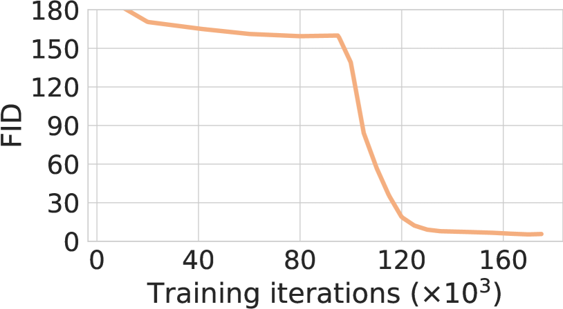
(a) CIFAR-10, NFE 2

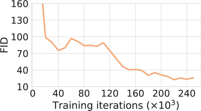
(b) AFHQ-Cat, NFE 6

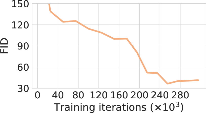
(c) CelebA-HQ, NFE 6

Figure 4: Demonstration of training convergence on three datasets.

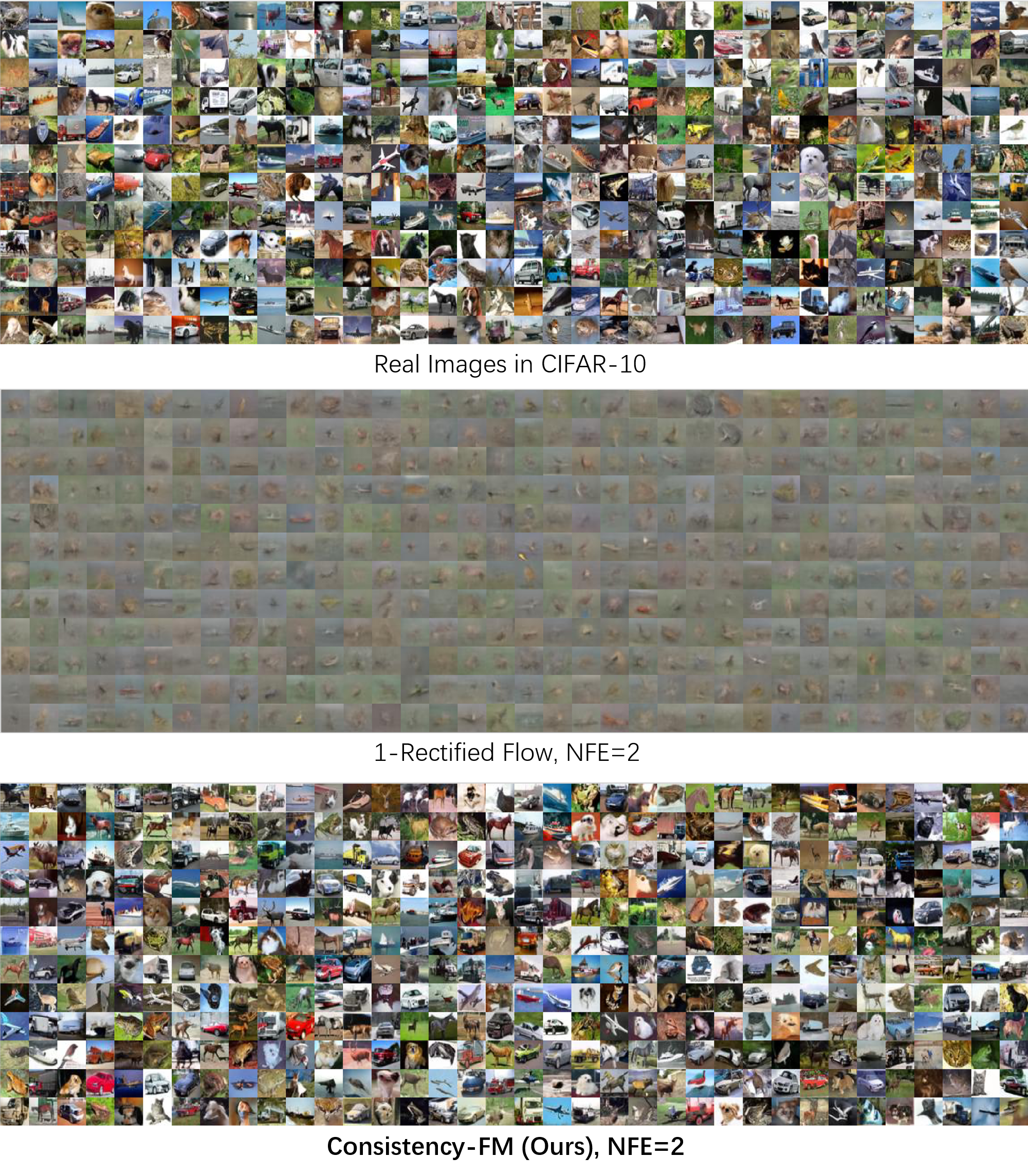
Figure 5: Sampling comparison between Rectified Flow [9] and our Consistency-FM.

5 Future Work

This work theoretically and empirically presents our new fundamental flow matching model. While we achieve some improvements in generated image quality and training efficiency. We here discuss a few directions for advancing this research:

• Text-to-image generation: While we demonstrates superior performance and efficiency on unconditional image generation, extending to large-scale datasets and more complex generation scenarios (e.g. text-to-image generation [54, 55, 3]) is necessary to further improve the capacity of our proposed velocity consistency.

• Distillation with pretrained models: In method part, we provide a loss function to distill pretrained FMs with our Consistency-FM. From a more general perspective, it is worth to explore whether our Consistency-FM is able to distill both pretrained DMs and FMs.

Appendix A Theoretical Supports and Proofs

A.1 PROOF OF LEMMA 1

Proof of Lemma 1.

If Condition 1 is meet, then ODE Eq. 1 associated with $v$ becomes

$$\frac{d\gamma_{x}(t)}{dt}=v(t,\gamma_{x}(t))=v(0,x),$$

and the solution of which is $\gamma_{x}(t)=x+t*v(0,x)$. Specifically, we have

$$\gamma_{x}(1) =x+1*v(0,x)$$

$$=\gamma_{x}(t)+(1-t)*v(0,\gamma_{x}(0))=\gamma_{x}(t)+(1-t)*v(t,\gamma_{x}(t))$$

$$=\gamma_{x}(s)+(1-s)*v(0,\gamma_{x}(0))=\gamma_{x}(s)+(1-s)*v(t,\gamma_{x}(s))$$

and thus Condition 2 is meet.

On the other hand, if Condition 2 is meet, then we have

$$\gamma_{x}(t)-\gamma_{x}(s) =(1-s)v(s,\gamma_{x}(s))-(1-t)v(t,\gamma_{x}(t))$$

$$=\int_{s}^{t}v(u,\gamma_{x}(u))du$$

Divide both hands in the above equation with $t-s$ and let $t$ approaches $s$, we have:

$$v(s,\gamma_{x}(s))=\lim_{t\to s}\frac{\int_{s}^{t}v(u,\gamma_{x}(u))du}{t-s},$$ (14)

$$=\lim_{t\to s}\frac{(1-s)v(s,\gamma_{x}(s))-(1-t)v(t,\gamma_{x}(t))}{t-s}$$

$$=\lim_{t\to s}v(t,\gamma_{x}(t))+(1-s)*\frac{v(s,\gamma_{x}(s))-v(t,\gamma_{x}(t))}{t-s}=v(s,\gamma_{x}(s))-(1-s)\frac{dv(s,\gamma_{s})}{ds}$$

Comparing the both sides in the above equation, we have $\frac{dv(s,\gamma_{s})}{ds}=0$, and thus Condition 1 is meet. ∎

A.2 PROOF OF LEMMA 2

We provide an another lemma which describes the consistency constraint as partial differential equations and supports the connection bewteen Consistency-FM with FMs.

Lemma 2.

Assume $v$ is continuously differentiable and consistent, then $v$ satisfies the following equation:

$$\partial_{t}v(t,x)+v\cdot\nabla_{x}v=0$$ (15)

Proof of Lemma 2.

By Lemma 1, if $v$ is consistent then it can be written as:

$$v(t+\Delta t,x_{t}+\Delta t*v(t,x_{t}))=v(t,x_{t})$$ (16)

Since $v$ is differentiable, we can take derivatives with respect to $t$:

$$\frac{dv}{dt}=\partial_{t}v+v\cdot\nabla_{x}v$$ (17)

Then by definition, if $v$ is consistent we have

$$\frac{dv}{dt}=\partial_{t}v+v\cdot\nabla_{x}v=0$$ (18)

∎

A.3 PROOF OF THEOREM 1

Proof of Theorem 1.

By the first mean value theorem, there exist a $t^{{}^{\prime}}\in[t,t+\Delta t]$, such that

$$x_{t+\Delta t}-x_{t}=\int_{t}^{t+\Delta t}u(s,x_{s})du=\Delta t*u(t^{{}^{\prime}},x_{t^{{}^{\prime}}})$$ (19)

Then by the definition of $f_{\theta}(t,x_{t})=x_{t}+(1-t)*v_{\theta}(t,x_{t})$, we have:

$$f_{\theta}(t,x_{t})-f_{\theta}(t+\Delta t,x_{t+\Delta t})$$ (20)

$$=x_{t}-x_{t+\Delta t}+(1-t)*v_{\theta}(t,x_{t})-(1-t-\Delta t)*v_{\theta}(t+\Delta t,x_{t+\Delta t}),$$

$$=\Delta t*v_{\theta}(t+\Delta t,x_{t+\Delta t})-\int_{t}^{t+\Delta t}u(s,x_{s})ds+(1-t)*(v_{\theta}(t,x_{t})-v_{\theta}(t+\Delta t,x_{t+\Delta t})),$$

$$=^{1}\Delta t*(v_{\theta}(t+\Delta t,x_{t+\Delta t})-u(t^{{}^{\prime}},x_{t^{{}^{\prime}}}))+(1-t)*(v_{\theta}(t,x_{t})-v_{\theta}(t+\Delta t,x_{t+\Delta t})),$$

$$=^{2}\Delta t*[((v_{\theta}(t+\Delta t,x_{t+\Delta t})-u(t^{\prime},x_{t^{\prime}}))-(1-t)(\partial_{t}v_{\theta}(t,x_{t})+u(t^{\prime},x_{t}^{\prime})\cdot\nabla_{x}v_{\theta}(t,x_{t}))]+O((\Delta t)^{2})$$

$$=^{3}\Delta t*[(v_{\theta}(t,x_{t})-u(t,x_{t}))-(1-t)(\partial_{t}v_{\theta}(t,x_{t})+u(t,x_{t})\cdot\nabla_{x}v_{\theta}(t,x_{t}))]+O((\Delta t)^{2}),$$

where in $(1)$ we used the first mean value theorem, in $(2)$ we used first-order Taylor approximation and in $(3)$ we used the boundedness of $v_{\theta}$, derivatives of $v_{\theta}$ and $u$. Then the objective can be written as:

$$E||f_{\theta}(t,x_{t})-f_{\theta}(t+\Delta t,x_{t+\Delta t})||_{2}^{2},$$

$$=E||\Delta t*(v_{\theta}(t,x_{t})-u(t,x_{t})-(1-t)(\partial_{t}v_{\theta}+u\cdot\nabla_{x}v_{\theta}))+O((\Delta t)^{2})||_{2}^{2}$$

$$=(\Delta t)^{2}*E||v_{\theta}(t,x_{t})-u(t,x_{t})-(1-t)(\partial_{t}v_{\theta}+u\cdot\nabla_{x}v_{\theta})||_{2}^{2}+o((\Delta t)^{2})$$

∎

A.4 PROOF OF THEOREM 2

Proof of Theorem 2.

As $v_{\theta}^{i}(t,x_{t})$ is the minimizer of Eq. 8 with respect to segment $i$, it must satisfies the first-order condition:

$$0 =\partial_{\theta}(E||f_{\theta}^{i}(t,x_{t})-f_{\theta^{-}}^{i}(t+\Delta t,x_{t+\Delta t})||_{2}^{2}+\alpha||v_{\theta}^{i}(t,x_{t})-v_{\theta^{-}}^{i}(t+\Delta t,x_{t+\Delta t})||_{2}^{2})$$ (21)

$$=E((T-t)(f_{\theta}^{i}(t,x_{t})-f_{\theta^{-}}^{i}(t+\Delta t,x_{t+\Delta t}))+\alpha(v_{\theta}^{i}(t,x_{t})-v_{\theta^{-}}^{i}(t+\Delta t,x_{t+\Delta t})))\cdot\partial_{\theta}v_{\theta}^{i}(t,x_{t}),$$

where $f_{\theta}^{i}(t,x_{t})=x_{t}+(T-t)v_{\theta}^{i}(t,x_{t})$ Note that in our assumption, $x_{t+\Delta t}$ is generated by an ODE and thus is a deterministic function of $(t,x_{t})$, then the non-trivial solution to 21 satisfies the following equation almost everywhere:

$$0=(T-t)(f_{\theta}^{i}(t,x_{t})-f_{\theta^{-}}^{i}(t+\Delta t,x_{t+\Delta t}))+\alpha(v_{\theta}^{i}(t,x_{t})-v_{\theta^{-}}^{i}(t+\Delta t,x_{t+\Delta t})),$$ (22)

As the gradient at $\theta$ is zero, then $\theta=\theta^{-}$, thus the learned velocity can be derived from 22:

$$v_{\theta}^{i}(t,x_{t})=\frac{(T-t)(x_{t+\Delta t}-x_{t})}{(T-t)^{2}+\alpha}+\frac{(T-t-\Delta t)(T-t)+\alpha}{(T-t)^{2}+\alpha}v_{\theta}^{i}(t+\Delta t,x_{t+\Delta t})$$ (23)

Furthermore, we have:

$$v_{\theta}^{i}(t,x_{t})$$ (24)

$$=\frac{(T-t)(x_{t+\Delta t}-x_{t})}{(T-t)^{2}+\alpha}+\frac{(T-t-\Delta t)(T-t)+\alpha}{(T-t)^{2}+\alpha}v^{*}(t+\Delta t,x_{t+\Delta t})$$

$$\quad+\frac{(T-t-\Delta t)(T-t)+\alpha}{(T-t)^{2}+\alpha}v_{\theta}^{i}(t+\Delta t,x_{t+\Delta t})-\frac{(T-t-\Delta t)(T-t)+\alpha}{(T-t)^{2}+\alpha}v^{*}(t+\Delta t,x_{t+\Delta t})$$

$$=\frac{(T-t)((T-(t+\Delta t))v^{*}(t+\Delta t,x_{t+\Delta t})+x_{t+\Delta t}-x_{t})}{(T-t)^{2}+\alpha}+\frac{\alpha v^{*}(t+\Delta t,x_{t+\Delta t})}{(T-t)^{2}+\alpha}$$

$$\quad+\frac{(T-t-\Delta t)(T-t)+\alpha}{(T-t)^{2}+\alpha}(v_{\theta}^{i}(t+\Delta t,x_{t+\Delta t})-v^{*}(t+\Delta t,x_{t+\Delta t}))$$

$$=^{1}\frac{(T-t)(x_{T}-x_{t})}{(T-t)^{2}+\alpha}+\frac{\alpha v^{*}(t+\Delta t,x_{t+\Delta t})}{(T-t)^{2}+\alpha}$$

$$\quad+\frac{(T-t-\Delta t)(T-t)+\alpha}{(T-t)^{2}+\alpha}(v_{\theta}^{i}(t+\Delta t,x_{t+\Delta t})-v^{*}(t+\Delta t,x_{t+\Delta t}))$$

$$=^{2}\frac{(T-t)^{2}v^{*}(t,x_{t})}{(T-t)^{2}+\alpha}+\frac{\alpha v^{*}(t+\Delta t,x_{t+\Delta t})}{(T-t)^{2}+\alpha}$$

$$\quad+\frac{(T-t-\Delta t)(T-t)+\alpha}{(T-t)^{2}+\alpha}(v_{\theta}^{i}(t+\Delta t,x_{t+\Delta t})-v^{*}(t+\Delta t,x_{t+\Delta t}))$$

$$=v^{*}(t,x_{t})+\frac{\alpha(v^{*}(t+\Delta t,x_{t+\Delta t})-v^{*}(t,x_{t}))}{(T-t)^{2}+\alpha}$$

$$\quad+\frac{(T-t-\Delta t)(T-t)+\alpha}{(T-t)^{2}+\alpha}(v_{\theta}^{i}(t+\Delta t,x_{t+\Delta t})-v^{*}(t+\Delta t,x_{t+\Delta t}))$$

where in (1) and (2) we have use the assumption of oracle $v^{*}$ that $x_{T}=x_{t}+(T-t)v^{*}(t,x_{t})$ ∎

A.5 PROOF OF COROLLARY 2.1

Proof for Corollary 2.1.

Note that $x_{T}=x_{T}+0*v_{\theta}^{i}(T,x_{T})$, and thus we can set arbitrary value for $v_{\theta}^{i}(T,x_{T})$ without affecting the model. Specifically, we set $v_{\theta}^{i}(T,x_{T})=v^{*}(T,x_{T})$. Then by Theorem 2, the error at $T-\Delta t$ is:

$$v_{\theta}^{i}(T-\Delta t,x_{T-\Delta t})-v^{*}(T-\Delta t,x_{T-\Delta t})$$ (25)

$$=\frac{\alpha}{(\Delta t)^{2}+\alpha}(v^{*}(T,x_{T})-v^{*}(T-\Delta t,x_{T-\Delta t}))$$

$$\quad+\frac{(\Delta t-\Delta t)(T-t)+\alpha}{(\Delta t)^{2}+\alpha}(v_{\theta}^{i}(T,x_{T})-v^{*}(T,x_{T}))$$

$$=\frac{\alpha}{(\Delta t)^{2}+\alpha}(v^{*}(T,x_{T})-v^{*}(T-\Delta t,x_{T-\Delta t}))$$

Furthermore, as $u$ is consistent within $[S,T]$, by Lemma 1 we have :

$$x_{T}=x_{t}+(T-t)*u(t,x_{t}),$$

$$\Rightarrow v^{*}(t,x_{t})=u(t,x_{t})\equiv u(T,x_{T}),$$

$$\Rightarrow v^{*}(t,x_{t})=v^{*}(t+\Delta t,x_{t+\Delta t}),\forall t\in[S,T-\Delta t].$$

And thus $v_{\theta}^{i}(T-\Delta t,x_{T-\Delta t})-v^{*}(T-\Delta t,x_{T-\Delta t})=0$.

By Theorem 2, we can deduce by induction that

$$v_{\theta}^{i}(t+\Delta t,x_{t+\Delta t})=v^{*}(t+\Delta t,x_{t+\Delta t})\quad\&\quad v^{*}(t,x_{t})=v^{*}(t+\Delta t,x_{t+\Delta t})$$

$$\Rightarrow v_{\theta}^{i}(t,x_{t})=v^{*}(t,x_{t})=u(t,x_{t}),\forall t\in[S,T-\Delta t].$$

∎

References

- [1] J. Ho, A. Jain, and P. Abbeel, “Denoising diffusion probabilistic models,” in NeurIPS, vol. 33, pp. 6840–6851, 2020.
- [2] L. Yang, Z. Zhang, Y. Song, S. Hong, R. Xu, Y. Zhao, W. Zhang, B. Cui, and M.-H. Yang, “Diffusion models: A comprehensive survey of methods and applications,” ACM Computing Surveys, vol. 56, no. 4, pp. 1–39, 2023.
- [3] L. Yang, Z. Yu, C. Meng, M. Xu, S. Ermon, and B. Cui, “Mastering text-to-image diffusion: Recaptioning, planning, and generating with multimodal llms,” in International Conference on Machine Learning, 2024.
- [4] L. Yang, Z. Zhang, Z. Yu, J. Liu, M. Xu, S. Ermon, and B. CUI, “Cross-modal contextualized diffusion models for text-guided visual generation and editing,” in International Conference on Learning Representations, 2024.
- [5] R. T. Chen, Y. Rubanova, J. Bettencourt, and D. K. Duvenaud, “Neural ordinary differential equations,” Advances in neural information processing systems, vol. 31, 2018.
- [6] Y. Song, C. Durkan, I. Murray, and S. Ermon, “Maximum likelihood training of score-based diffusion models,” Advances in neural information processing systems, vol. 34, pp. 1415–1428, 2021.
- [7] Y. Lipman, R. T. Chen, H. Ben-Hamu, M. Nickel, and M. Le, “Flow matching for generative modeling,” in The Eleventh International Conference on Learning Representations, 2022.
- [8] M. S. Albergo and E. Vanden-Eijnden, “Building normalizing flows with stochastic interpolants,” in The Eleventh International Conference on Learning Representations, 2022.
- [9] X. Liu, C. Gong, et al., “Flow straight and fast: Learning to generate and transfer data with rectified flow,” in The Eleventh International Conference on Learning Representations, 2022.
- [10] Y. Song and S. Ermon, “Generative modeling by estimating gradients of the data distribution,” Advances in neural information processing systems, vol. 32, 2019.
- [11] X. Liu, X. Zhang, J. Ma, J. Peng, and Q. Liu, “Instaflow: One step is enough for high-quality diffusion-based text-to-image generation,” arXiv preprint arXiv:2309.06380, 2023.
- [12] N. Kornilov, A. Gasnikov, and A. Korotin, “Optimal flow matching: Learning straight trajectories in just one step,” arXiv preprint arXiv:2403.13117, 2024.
- [13] A. Tong, N. Malkin, G. Huguet, Y. Zhang, J. Rector-Brooks, K. FATRAS, G. Wolf, and Y. Bengio, “Improving and generalizing flow-based generative models with minibatch optimal transport,” in ICML Workshop on New Frontiers in Learning, Control, and Dynamical Systems, 2023.
- [14] A.-A. Pooladian, H. Ben-Hamu, C. Domingo-Enrich, B. Amos, Y. Lipman, and R. T. Chen, “Multisample flow matching: Straightening flows with minibatch couplings,” 2023.
- [15] Y. Song, P. Dhariwal, M. Chen, and I. Sutskever, “Consistency models,” in International Conference on Machine Learning, pp. 32211–32252, PMLR, 2023.
- [16] B. Nguyen, B. Nguyen, and V. A. Nguyen, “Bellman optimal stepsize straightening of flow-matching models,” in The Twelfth International Conference on Learning Representations, 2024.
- [17] D. Kim, C.-H. Lai, W.-H. Liao, N. Murata, Y. Takida, T. Uesaka, Y. He, Y. Mitsufuji, and S. Ermon, “Consistency trajectory models: Learning probability flow ode trajectory of diffusion,” in The Twelfth International Conference on Learning Representations, 2023.
- [18] L. Klein, A. Krämer, and F. Noe, “Equivariant flow matching,” in Thirty-seventh Conference on Neural Information Processing Systems, 2023.
- [19] H. Stark, B. Jing, C. Wang, G. Corso, B. Berger, R. Barzilay, and T. Jaakkola, “Dirichlet flow matching with applications to dna sequence design,” arXiv preprint arXiv:2402.05841, 2024.
- [20] A. Campbell, J. Yim, R. Barzilay, T. Rainforth, and T. Jaakkola, “Generative flows on discrete state-spaces: Enabling multimodal flows with applications to protein co-design,” arXiv preprint arXiv:2402.04997, 2024.
- [21] A. Makkuva, A. Taghvaei, S. Oh, and J. Lee, “Optimal transport mapping via input convex neural networks,” in International Conference on Machine Learning, pp. 6672–6681, PMLR, 2020.
- [22] M. Arjovsky, S. Chintala, and L. Bottou, “Wasserstein generative adversarial networks,” in International conference on machine learning, pp. 214–223, PMLR, 2017.
- [23] I. Goodfellow, J. Pouget-Abadie, M. Mirza, B. Xu, D. Warde-Farley, S. Ozair, A. Courville, and Y. Bengio, “Generative adversarial nets,” Advances in neural information processing systems, vol. 27, 2014.
- [24] D. P. Kingma and M. Welling, “Auto-encoding variational bayes,” arXiv preprint arXiv:1312.6114, 2013.
- [25] Y. Song, J. Sohl-Dickstein, D. P. Kingma, A. Kumar, S. Ermon, and B. Poole, “Score-based generative modeling through stochastic differential equations,” in International Conference on Learning Representations, 2020.
- [26] J. Song, C. Meng, and S. Ermon, “Denoising diffusion implicit models,” in International Conference on Learning Representations, 2020.
- [27] D. Rezende and S. Mohamed, “Variational inference with normalizing flows,” in International conference on machine learning, pp. 1530–1538, PMLR, 2015.
- [28] L. Dinh, J. Sohl-Dickstein, and S. Bengio, “Density estimation using real nvp,” in International Conference on Learning Representations, 2016.
- [29] F. Bao, C. Li, J. Zhu, and B. Zhang, “Analytic-dpm: an analytic estimate of the optimal reverse variance in diffusion probabilistic models,” in International Conference on Learning Representations, 2021.
- [30] T. Dockhorn, A. Vahdat, and K. Kreis, “Score-based generative modeling with critically-damped langevin diffusion,” in International Conference on Learning Representations, 2021.
- [31] Z. Xiao, K. Kreis, and A. Vahdat, “Tackling the generative learning trilemma with denoising diffusion gans,” in International Conference on Learning Representations, 2021.
- [32] C. Lu, Y. Zhou, F. Bao, J. Chen, C. Li, and J. Zhu, “Dpm-solver: A fast ode solver for diffusion probabilistic model sampling in around 10 steps,” in Advances in Neural Information Processing Systems.
- [33] T. Dockhorn, A. Vahdat, and K. Kreis, “GENIE: Higher-Order Denoising Diffusion Solvers,” Advances in Neural Information Processing Systems, 2022.
- [34] H. Zheng, W. Nie, A. Vahdat, K. Azizzadenesheli, and A. Anandkumar, “Fast sampling of diffusion models via operator learning,” in International Conference on Machine Learning, pp. 42390–42402, PMLR, 2023.
- [35] T. Salimans and J. Ho, “Progressive distillation for fast sampling of diffusion models,” in International Conference on Learning Representations, 2022.
- [36] W. Luo, T. Hu, S. Zhang, J. Sun, Z. Li, and Z. Zhang, “Diff-instruct: A universal approach for transferring knowledge from pre-trained diffusion models,” Advances in Neural Information Processing Systems, vol. 36, 2024.
- [37] W. Luo, “A comprehensive survey on knowledge distillation of diffusion models,” arXiv preprint arXiv:2304.04262, 2023.
- [38] Y. Song and P. Dhariwal, “Improved techniques for training consistency models,” arXiv preprint arXiv:2310.14189, 2023.
- [39] C. Villani et al., Optimal transport: old and new, vol. 338. Springer, 2009.
- [40] S. Lee, B. Kim, and J. C. Ye, “Minimizing trajectory curvature of ode-based generative models,” in International Conference on Machine Learning, pp. 18957–18973, PMLR, 2023.
- [41] P. Esser, S. Kulal, A. Blattmann, R. Entezari, J. Müller, H. Saini, Y. Levi, D. Lorenz, A. Sauer, F. Boesel, et al., “Scaling rectified flow transformers for high-resolution image synthesis,” arXiv preprint arXiv:2403.03206, 2024.
- [42] J. C. Butcher, Numerical methods for ordinary differential equations. John Wiley & Sons, 2016.
- [43] K. Alex, “Learning multiple layers of features from tiny images,” https://www. cs. toronto. edu/kriz/learning-features-2009-TR. pdf, 2009.
- [44] T. Karras, T. Aila, S. Laine, and J. Lehtinen, “Progressive growing of gans for improved quality, stability, and variation,” arXiv preprint arXiv:1710.10196, 2017.
- [45] Y. Choi, Y. Uh, J. Yoo, and J.-W. Ha, “Stargan v2: Diverse image synthesis for multiple domains,” in Proceedings of the IEEE/CVF conference on computer vision and pattern recognition, pp. 8188–8197, 2020.
- [46] M. Heusel, H. Ramsauer, T. Unterthiner, B. Nessler, and S. Hochreiter, “Gans trained by a two time-scale update rule converge to a local nash equilibrium,” Advances in neural information processing systems, vol. 30, 2017.
- [47] A. Vahdat, K. Kreis, and J. Kautz, “Score-based generative modeling in latent space,” Advances in neural information processing systems, vol. 34, pp. 11287–11302, 2021.
- [48] Y. Xu, Z. Liu, M. Tegmark, and T. Jaakkola, “Poisson flow generative models,” Advances in Neural Information Processing Systems, vol. 35, pp. 16782–16795, 2022.
- [49] T. Karras, M. Aittala, T. Aila, and S. Laine, “Elucidating the design space of diffusion-based generative models,” Advances in Neural Information Processing Systems, vol. 35, pp. 26565–26577, 2022.
- [50] D. P. Kingma and P. Dhariwal, “Glow: Generative flow with invertible 1x1 convolutions,” Advances in neural information processing systems, vol. 31, 2018.
- [51] R. T. Chen, J. Behrmann, D. K. Duvenaud, and J.-H. Jacobsen, “Residual flows for invertible generative modeling,” Advances in Neural Information Processing Systems, vol. 32, 2019.
- [52] Z. Xiao, Q. Yan, and Y. Amit, “Generative latent flow,” arXiv preprint arXiv:1905.10485, 2019.
- [53] M. Grcić, I. Grubišić, and S. Šegvić, “Densely connected normalizing flows,” Advances in Neural Information Processing Systems, vol. 34, pp. 23968–23982, 2021.
- [54] R. Rombach, A. Blattmann, D. Lorenz, P. Esser, and B. Ommer, “High-resolution image synthesis with latent diffusion models,” in CVPR, pp. 10684–10695, 2022.
- [55] D. Podell, Z. English, K. Lacey, A. Blattmann, T. Dockhorn, J. Müller, J. Penna, and R. Rombach, “Sdxl: Improving latent diffusion models for high-resolution image synthesis,” arXiv preprint arXiv:2307.01952, 2023.