The weak form of the SDOF and MDOF equation of motion, part II: A numerical method for the SDOF problem

Abstract

A new, more efficient, numerical method for the SDOF problem is presented. Its construction is based on the weak form of the equation of motion, as obtained in [KK24], using piece-wise polynomial functions as interpolation functions. The approximation rate can be arbitrarily high, proportional to the degree of the interpolation functions, tempered only by numerical instability. Moreover, the mechanical energy of the system is conserved. Consequently, all significant drawbacks of existing algorithms, such as the limitations imposed by the Dahlqvist Barrier theorem [Dah56] and the need for introduction of numerical damping, have been overcome.

1 Application of the weak formulation to piece-wise polynomial interpolation

The algorithm presented herein, based on the weak formulation of the SDOF problem as obtained in [KK24], is constructed as follows. A partition of the interval $[0,\bar{T}]$ into $l$ intervals of length $h$ is considered, and the approximate solution $x_{ap}$ will be polynomial in each subinterval of the type

$$I_{j}=[jh,(j+1)h]$$ (1)

The space formed by such functions will be denoted by $\mathcal{P}_{h,p}=\mathcal{P}_{h,p}([0,\bar{T}])$.

The breakpoints $\{jh\}_{j=0\cdots l}$, i.e. the points where the expression of a function in $\mathcal{P}_{h,p}$ is allowed to change are equally spaced in $I$, and the corresponding time-step is $h>0$. The time-step $h$ is chosen so that

$$\frac{\bar{T}}{h}=l\in\mathbb{N}^{*}$$ (2)

where $l$ is the number of time-steps of the algorithm.

The functions $B_{i,p,h}$, defined here below, for some fixed $p\geq 3$, will form a basis for the restriction of functions in $\mathcal{P}_{h,p}$ in each subinterval formed by consecutive break-points. The weak formulation of the SDOF problem will be considered in each such interval $I_{j}$. The algorithm thus takes automatically a time-step algorithm character and, even though it does not represent the full potential of the weak formulation, can be seen to be already more powerful than those in the literature.

Consequently, there is some change in notation with respect to [KK24], since $\bar{T}$ still stands for the upper bound of the interval in which the solution is approximated, but the intervals on which the weak formulation is considered are precisely the $I_{j}$, for $j=0,\cdots,l-1$ where $l=\bar{T}/h\in\mathbb{N}^{*}$.

The authors are already working on the construction of a numerical method based on the weak formulation on the entire interval $[0,\bar{T}]$, which will also have a step-by-step nature.

2 Choice of functions

Fix $h>0$. The space

$$\mathcal{P}=\mathcal{P}(p,h)\subset H^{1}([0,h])$$ (3)

is chosen to be equal to the space of polynomial functions of a given degree $p-1\in\mathbb{N}^{*}$, $p\geq 3$. It is of dimension $p$. The space

$$\dot{\mathcal{P}}=\dot{\mathcal{P}}(p,h)=\{\dot{\varphi},\varphi\in\mathcal{P}(p,h)\}\subset H^{1}([0,h])$$ (4)

is thus equal to the space of polynomial functions of degree $p-2\in\mathbb{N}^{*}$ and of dimension $p-1$.

The basis of $\mathcal{P}$ given in the next equation is known in the literature as the Bernstein polynomials, see, e.g., [Kac38]. Call, for $i=1,\cdots,p$,

$$B_{i,p,h}(t)=B_{i}(t)=\begin{cases}\frac{\Gamma(p)}{\Gamma(i)\Gamma(p-i+1)}\left(\frac{t}{h}\right)^{i-1}\left(\frac{h-t}{h}\right)^{p-i}\text{ if }0\leq t\leq h\\ 0\hphantom{\frac{\Gamma(p)}{\Gamma(i)-}\left(\frac{t}{h}\right)^{i-1}}\text{ otherwise}\end{cases}$$ (5)

All functions $B_{i}$ are by their definition non-negative. The normalization factor

$$\frac{\Gamma(p)}{\Gamma(i)\Gamma(p-i+1)}={{p-1}\choose{i-1}}=\frac{(p-1)!}{(i-1)!(p-i)!}$$ (6)

is chosen so that

$$\sum_{i=1}^{p}B_{i}(t)=\begin{cases}1\text{ if }0\leq t\leq h\\ 0\text{ otherwise}\end{cases}$$ (7)

i.e. so that the $B_{i}$ form a partition of unity on the interval $[0,h]$ (cf. [dB78], §IX).

3 Some useful properties of Bernstein polynomials

3.1 The functions and their derivatives

The Bernstein polynomials form a basis of polynomial functions of degree $p-1$ defined on $[0,h]$. For this particular choice of basis, one can immediately verify that

$$\begin{array}[]{l@{}l}B_{i}(0)\neq 0&\iff i=1\\ B_{i}(h)\neq 0&\iff i=p\\ B_{i}^{\prime}(0)\neq 0&\iff i\in\{1,2\}\\ B_{i}^{\prime}(h)\neq 0&\iff i\in\{p-1,p\}\\ \end{array}$$ (8)

More precisely,

$$\begin{array}[]{l@{}l}B_{1}(0)=B_{p}(h)&=1\\ B_{1}^{\prime}(0)=-B_{p}^{\prime}(h)&=-\frac{p-1}{h}\\ B_{2}(0)=B_{p-1}(h)&=0\\ B_{2}^{\prime}(0)=-B_{p-1}^{\prime}(h)&=\frac{p-1}{h}\end{array}$$ (9)

The following lemma will be useful for the calculation of the derivatives of Bernstein polynomials. The derivative of a polynomial of degree $p$ is a polynomial of degree $p-1$. The following lemma shows how to express a Bernstein polynomial of degree $p-1$ in terms of Bernstein polynomials of degree $p$.

Lemma 3.1.

The following formula holds true for $i=1,\cdots,p-1$:

$$B_{i,p-1,h}(t)=\frac{p-i}{p-1}B_{i,p,h}(t)+\frac{i}{p-1}B_{i+1,p,h}(t)$$ (10)

Proof.

The proof is elementary and is based on the following observation:

$$\begin{array}[]{r@{}l}\left(\frac{t}{h}\right)^{i-1}\left(\frac{h-t}{h}\right)^{p-i}+\left(\frac{t}{h}\right)^{i}\left(\frac{h-t}{h}\right)^{p-i-1}&=\left(\frac{t}{h}\right)^{i-1}\left(\frac{h-t}{h}\right)^{p-i-1}\left(\frac{t}{h}+\frac{h-t}{h}\right)\\ &=\left(\frac{t}{h}\right)^{i-1}\left(\frac{h-t}{h}\right)^{p-i-1}\\ &={{p-2}\choose{i-1}}^{-1}B_{i,p-1,h}(t)\end{array}$$ (11)

and the rest is a direct calculation involving the normalization factors. ∎

The following lemma is elementary. The proof is by immediate calculation and use of lemma 3.1.

Lemma 3.2.

The following formula holds true for $i=1,\cdots,p$, where for convenience, for all $p\in\mathbb{N}^{*}$, $B_{0,p,h}(t)\equiv B_{p+1,p,h}(t)\equiv 0$:

$$\begin{array}[]{r@{}l}\frac{d}{dt}B_{i,p,h}(t)&=\frac{p-1}{h}(B_{i-1,p-1,h}(t)-B_{i,p-1,h}(t))\\ &=\frac{1}{h}((p-i-1)B_{i-1,p,h}(t)+(2i-p-1)B_{i,p,h}(t)-iB_{i+1,p,h}(t))\end{array}$$ (12)

The following corollary follows from direct calculation.

Corollary 3.3.

The local maximum of $B_{i,p,h}$ for $i=2,\cdots,p-1$ is attained at $t=\frac{ih}{p}$

Proof.

From the formula of the lemma it easily follows that

$$\frac{d}{dt}B_{i,p,h}(t)=\frac{(p-1)!}{i!(p-i)!}\left(\frac{t}{h}\right)^{i-1}\left(\frac{h-t}{h}\right)^{p-i-1}\frac{ih-pt}{h}$$ (13)

whose only root inside $(0,h)$ is $t=\frac{ih}{p}$ and the corollary follows. ∎

3.1.1 Integrals and $L^{2}$ products

The following lemma concerns the integral of a Bernstein polynomial. It will be useful for the calculation of $L^{2}_{c}$ scalar products.

Lemma 3.4.

The integral of a Bernstein polynomial $B_{i,p,h}$ over $[0,h]$ depends only on $p$ and $h$:

$$\int_{0}^{h}B_{i,p,h}(t)\mathrm{d}t=\frac{h}{p}$$ (14)

Proof.

The proof can proceed by integration by parts. Alternatively, lemma 3.2 implies that, for $i=1,\cdots,p$,

$$\begin{array}[]{r@{}l}\int_{0}^{h}(B_{i-1,p,h}(t)-B_{i,p,h}(t))dt&=\frac{h}{p}\int_{0}^{h}\frac{d}{dt}B_{i,p+1,h}(t)\mathrm{d}t\\ &=\frac{h}{p}(B_{i,p+1,h}(h)-B_{i,p+1,h}(0))\\ &=\frac{h}{p}(\delta_{i,p+1}-\delta_{i,1})\end{array}$$ (15)

where $\delta_{kl}$ is the Kronecker delta function, equal to $1$ if $k=l$ and $0$ otherwise. The conclusion of the lemma follows directly by using the fact that the Bernstein polynomials form a partition of unity, which implies that

$$\sum_{i=1}^{p}\int_{0}^{h}B_{i,p,h}(t)\mathrm{d}t=h$$ (16)

from which the conclusion follows easily. ∎

A formula for indefinite integrals of Bernstein polynomials can also be obtained. The proof is by integration by parts and application of lemma 3.9 for $q=1$.

Lemma 3.5.

It holds true that

$$\begin{array}[]{r@{}l}\int_{0}^{t}B_{i,p,h}(\tau)\mathrm{d}\tau&=\frac{h}{p}\sum_{j=i+1}^{p+1}B_{j,p+1,h}(t)\\ &=\frac{h}{p}\left(1-\sum_{j=1}^{i}B_{j,p+1,h}(t)\right)\end{array}$$ (17)

Proof.

Direct calculation gives

$$\begin{array}[]{r@{}l}\int_{0}^{t}B_{i,p,h}(\tau)\mathrm{d}\tau&=tB_{i,p,h}(t)-\int_{0}^{t}\tau\dot{B}_{i,p,h}(\tau)\mathrm{d}\tau\\ &=h\frac{i}{p}B_{i+1,p+1,h}(t)-\frac{p-1}{h}\int_{0}^{t}\tau(B_{i-1,p-1,h}(\tau)-B_{i,p-1,h}(\tau))\mathrm{d}\tau\\ &=h\frac{i}{p}B_{i+1,p+1,h}(t)-(i-1)\int_{0}^{t}B_{i,p,h}(\tau)\mathrm{d}\tau+i\int_{0}^{t}\tau B_{i+1,p,h}(\tau)\mathrm{d}\tau\end{array}$$ (18)

so that, all in all,

$$\int_{0}^{t}B_{i,p,h}(\tau)\mathrm{d}\tau=\frac{h}{p}B_{i+1,p+1,h}(t)+\int_{0}^{t}B_{i+1,p,h}(\tau)\mathrm{d}\tau$$ (19)

It can be seen directly, either by calculation or by the standing convention that $B_{p+1,p,h}\equiv 0$, that

$$\int_{0}^{t}B_{p,p,h}(\tau)\mathrm{d}\tau=\frac{h}{p}B_{p+1,p+1,h}(t)$$ (20)

so that, for all $1\leq i\leq p$,

$$\int_{0}^{t}B_{i,p,h}(\tau)\mathrm{d}\tau=\frac{h}{p}\sum_{j=i+1}^{p+1}B_{j,p+1,h}(t)$$ (21)

In particular, lemma 3.4 can be obtained by this formula.

The last part follows from the fact that the Bernstein polynomials form a partition of unity. ∎

The product of two Bernstein polynomials satisfies the following simple rule, the proof of which is left to the reader.

Lemma 3.6.

It holds true that, for $1\leq i\leq p$ and $1\leq j\leq q$ and $h>0$,

$$B_{i,p,h}(t)B_{j,q,h}(t)=\frac{{{p-1}\choose{i-1}}{{q-1}\choose{j-1}}}{{{p+q-2}\choose{i+j-2}}}B_{i+j-1,p+q-1,h}(t)$$ (22)

Combining lemmas 3.4 and 3.6 directly yields the following corollary. For notation, the reader is referred to eq. (22) of [KK24].

Corollary 3.7.

The $L^{2}_{0}$ scalar product of two Bernstein polynomials is given by

$$\langle B_{i,p,h}(\cdot),B_{j,q,h}(\cdot)\rangle_{0}=\int_{0}^{h}B_{i,p,h}(\cdot)B_{j,q,h}(\cdot)=\frac{{{p-1}\choose{i-1}}{{q-1}\choose{j-1}}}{(p+q-1){{p+q-2}\choose{i+j-2}}}h$$ (23)

The $L^{2}_{0}$ norm of a Bernstein polynomial is given by

$$\|B_{i,p,h}(\cdot)\|_{L^{2}_{0}}=\left(\langle B_{i,p,h}(\cdot),B_{i,p,h}(\cdot)\rangle_{0}\right)^{1/2}=\frac{{{p-1}\choose{i-1}}}{\sqrt{(2p-1){{2p-2}\choose{2i-2}}}}\sqrt{h}$$ (24)

A numerical estimation of the behavior of products is given in the following lemma.

Lemma 3.8.

For $3\leq p\leq 200$ it holds true that

$$\begin{array}[]{r@{}l}\max\limits_{1\leq i,j\leq p}\langle B_{i,p,h}(\cdot),B_{j,p,h}(\cdot)\rangle_{0}&\leq\frac{h}{p^{11/10}}\end{array}$$ (25)

In particular, since

$$t^{q}=h^{q}B_{q+1,q+1,h}(t)\text{ for }t\in[0,h]$$ (26)

one gets directly the following lemma, concerning the moments of the Bernstein polynomials. It will be useful in the estimation of $L^{2}_{c}$ scalar products, using the formula for the $L^{2}_{0}$ scalar product.

Lemma 3.9.

For $1\leq i\leq p$ and $h>0$,

$$\begin{array}[]{r@{}l}t^{q}B_{i,p,h}(t)&=h^{q}\frac{{{p-1}\choose{i-1}}}{{{p+q-1}\choose{i+q-1}}}B_{i+q,p+q,h}(t)\\ &=h^{q}\frac{{i^{(q)}}}{p^{(q)}}B_{i+q,p+q,h}(t)\end{array}$$ (27)

In the notation of the lemma,

$$\begin{array}[]{r@{}l}i^{(0)}&=1\\ i^{(q)}&=i(i+1)(i+2)\cdots(i+q-1)\end{array}$$ (28)

is the rising factorial and the following identity was used.

$$\frac{{(i-1)^{(q)}}}{(p-1)^{(q)}}=\frac{{{p-1}\choose{i-1}}}{{{p+q-1}\choose{i+q-1}}}$$ (29)

The following lemma can now be proven.

Lemma 3.10.

Let $c\geq 0$ and $h>0$. Then, the $L^{2}_{c}$ scalar product of two Bernstein polynomials is given by

$$\begin{array}[]{r@{}l}\langle B_{i,p,h}(\cdot),B_{j,q,h}(\cdot)\rangle_{c}&=\int_{0}^{h}e^{c\cdot}B_{i,p,h}(\cdot)B_{j,q,h}(\cdot)=\\ &={{p-1}\choose{i-1}}{{q-1}\choose{j-1}}\sum\limits_{n=0}^{\infty}\frac{c^{n}h^{n+1}}{n!}\frac{1}{(p+q+n-1){{p+q+n-2}\choose{i+j+n-2}}}\\ &=h\frac{{{p-1}\choose{i-1}}{{q-1}\choose{j-1}}}{(p+q-1){{p+q-2}\choose{i+j-2}}}{}_{1}F_{1}(i+j-1,p+q,ch)\end{array}$$ (30)

The $L^{2}_{c}$ norm of a Bernstein polynomial is given by

$$\begin{array}[]{r@{}l}\|B_{i,p,h}(\cdot)\|_{L^{2}_{c}}^{2}&=\left(\langle B_{i,p,h}(\cdot),B_{i,p,h}(\cdot)\rangle_{c}\right)=\\ &={{p-1}\choose{i-1}}^{2}\sum\limits_{n=0}^{\infty}\frac{c^{n}h^{n+1}}{n!}\frac{1}{(2p+n-1){{2p+n-2}\choose{2i+n-2}}}\\ &=h\frac{{{p-1}\choose{i-1}}^{2}}{(2p-1){{2p-2}\choose{2i-2}}}{}_{1}F_{1}(2i-1,2p,ch)\end{array}$$ (31)

In statement of the lemma, Kummer’s confluent hypergeometric function is used, which is defined as

$$\begin{array}[]{r@{}l}{}_{1}F_{1}(a;b;z)&=\sum_{n=0}^{\infty}\frac{a^{(n)}z^{n}}{b^{(n)}n!}\\ &=\frac{\Gamma(b)}{\Gamma(a)\Gamma(b-a)}\int_{0}^{1}e^{zu}u^{a-1}(1-u)^{b-a-1}\mathrm{d}u\end{array}$$ (32)

where the rising factorial is defined in eq. (28), and the integral representation holds in the domain $\mathrm{Re}(a)>0$ and $\mathrm{Re}(b)>0$, which is the case of interest for the lemma.

The proof of lemma uses the power-series expansion of the exponential,

$$e^{t}=\sum_{0}^{\infty}\frac{1}{n!}t^{n}$$ (33)

lemma 3.6 and its corollary. Both the lemma and its corollary are, of course, special cases of this lemma, obtained by posing $c=0$ (where the formal convention $c^{0}=1$ when $c=0$ is used).

Proof.

By definition and by lemmas 3.4, 3.6 and 3.9,

$$\begin{array}[]{r@{}l}\langle B_{i,p,h}(\cdot),B_{j,q,h}(\cdot)\rangle_{c}&=\int_{0}^{h}e^{ct}B_{i,p,h}(t)B_{j,q,h}(t)\mathrm{d}t\\ &=\int_{0}^{h}\sum\limits_{n=0}^{\infty}\frac{1}{n!}(ct)^{n}B_{i,p,h}(t)B_{j,q,h}(t)\mathrm{d}t\\ &=\sum\limits_{n=0}^{\infty}\frac{c^{n}}{n!}\int_{0}^{h}t^{n}B_{i,p,h}(t)B_{j,q,h}(t)\mathrm{d}t\\ &=\frac{{{p-1}\choose{i-1}}{{q-1}\choose{j-1}}}{{{p+q-2}\choose{i+j-2}}}\sum\limits_{n=0}^{\infty}\frac{c^{n}}{n!}\int_{0}^{h}t^{n}B_{i+j-1,p+q-1,h}(t)\mathrm{d}t\\ &=\frac{{{p-1}\choose{i-1}}{{q-1}\choose{j-1}}}{{{p+q-2}\choose{i+j-2}}}\sum\limits_{n=0}^{\infty}\frac{c^{n}h^{n}}{n!}\frac{{{p+q-2}\choose{i+j-2}}}{{{p+q+n-2}\choose{i+j+n-2}}}\int_{0}^{h}B_{i+j+n-1,p+q+n-1,h}(t)\mathrm{d}t\\ &={{p-1}\choose{i-1}}{{q-1}\choose{j-1}}\sum\limits_{n=0}^{\infty}\frac{c^{n}h^{n+1}}{n!}\frac{1}{(p+q+n-1){{p+q+n-2}\choose{i+j+n-2}}}\end{array}$$ (34)

The expression using Kummer’s confluent hypergeometric function follows from direct application of the power series definition, or the integral formula and the definition of the Bernstein polynomials. The series converges as it is bounded above by the exponential series. ∎

The proof of the previous lemma also provides a calculation for the product of an exponential with a Bernstein polynomial and its expression in the Bernstein polynomial basis. It is stated in the form of a lemma for convenience.

Lemma 3.11.

The following formula holds true

$$\begin{array}[]{r@{}l}e^{c\cdot}B_{i,p,h}(\cdot)&={{p-1}\choose{i-1}}\sum\limits_{n=0}^{\infty}\frac{c^{n}h^{n}}{n!}\frac{1}{{{p+n-1}\choose{i+n-1}}}B_{i+n,p+n,h}(t)\\ &=\sum\limits_{n=0}^{\infty}\frac{c^{n}h^{n}}{n!}\frac{i^{(n)}}{p^{(n)}}B_{i+n,p+n,h}(t)\end{array}$$ (35)

It is reminded that the rising factorial is defined in eq. (28). The following corollary also follows directly.

Corollary 3.12.

The integral of a Bernstein polynomial multiplied by an exponential is given by

$$\int_{0}^{t}e^{c\tau}B_{i,p,h}(\tau)\mathrm{d}\tau=\frac{h}{p}\sum\limits_{n=0}^{\infty}\frac{c^{n}h^{n}}{n!}\frac{i^{(n)}}{(p+1)^{(n)}}\sum_{j=i+n+1}^{p+n+1}B_{j,p+n+1,h}(t)$$ (36)

and its definite integral by

$$\begin{array}[]{r@{}l}\int_{0}^{h}\int_{0}^{t}e^{c\tau}B_{i,p,h}(\tau)\mathrm{d}\tau\mathrm{d}t&=\frac{h^{2}(p-i+1)}{p(p+1)}\sum\limits_{n=0}^{\infty}\frac{c^{n}h^{n}}{n!}\frac{i^{(n)}}{(p+2)^{(n)}}\\ &=\frac{h^{2}(p-i+1)}{p(p+1)}{}_{1}F_{1}(i,p+2,ch)\end{array}$$ (37)

3.2 Polynomial approximation of functions in Sobolev spaces

In the following, theorems $2.3$ and $2.4$ from [CQ82] will be needed. For completeness, the statements and the context of the needed results are presented here below.

In the proof, the Legendre basis for the space of polynomials of degree $p-1$ is more useful than the Bernstein polynomials, due to their property of being orthogonal with respect to the $L^{2}$-norm when restricted in the interval $(-1,1)$. The Legendre polynomials have a number of possible expressions, both implicit and explicit, one of them being

$$L_{n}(x)=\frac{1}{2^{n}n!}\frac{\mathrm{d}^{n}}{\mathrm{d}x}(x^{2}-1)^{n}$$ (38)

The polynomial $L_{n}(\cdot)$ is of degree $n$ and satisfies

$$\begin{array}[]{r@{}l}L_{n}(1)&=1\\ \int_{-1}^{1}L_{n}(\cdot)L_{m}(\cdot)&=0,\forall m\neq n\\ \|L_{n}\|_{L^{2}}^{2}&=\frac{2}{2n+1}\end{array}$$ (39)

so that

$$\phi_{n}(\cdot)=\sqrt{\frac{2n+1}{2}}L_{n}(\cdot),n\in\mathbb{N}$$ (40)

form a complete orthonormal basis for $L^{2}(-1,1)$.

For $p\geq 1$, the Legendre basis is given by

$$\{\phi_{n}\}_{n=0,\cdots p-1}$$ (41)

and is thus equivalent to the Bernstein basis, obtained by $\{B_{i,p,1}(\cdot)\}_{i=1,\cdots,p}$ after a transformation of the domain of the $B_{i,p,1}$ (which are defined on $[0,1]$), see [Far00] for a study of the basis transformations.

A function $u\in L^{2}(-1,1)$ admits the Fourier-Legendre representation

$$u(\cdot)=\sum_{0}^{\infty}u_{n}\phi_{n}(\cdot)$$ (42)

where $u_{k}=\int_{-1}^{1}u(\cdot)\phi_{n}(\cdot)$ and the orthogonal projection on the space of polynomials of degree $p-1$ is given by

$$T_{p}u(\cdot)=\sum_{0}^{p-1}u_{n}\phi_{n}(\cdot)$$ (43)

With this notation, the following statements hold. They consist in a simple rephrasing of the corresponding statements in the reference [CQ82]. To each statement a corollary is given, obtained just by transforming the interval $[-1,1]$ to the interval $[0,h]$, which is of interest in the present article. The proof of the corollaries is omitted, as it follows directly from the transformation of functions and integrals under composition with affine transformations.

Theorem 3.13 (Theorem $2.3$ of [CQ82]).

For any real $\sigma\geq 0$, there exists a constant $C$ such that for any $p\in\mathbb{N}$,

$$\|u-T_{p}u\|_{L^{2}(-1,1)}\leq C(p+1)^{-\sigma}\|u\|_{H^{\sigma}(-1,1)},\forall u\in H^{\sigma}(-1,1)$$ (44)

Corollary 3.14.

For any real $\sigma\geq 0$, there exists a constant $C$ such that for any $p\in\mathbb{N}$,

$$\|u-T_{p}u\|_{L^{2}(0,h)}\leq C(p+1)^{-\sigma}h^{\sigma}\|u\|_{H^{\sigma}(0,h)}$$ (45)

for all $u\in H^{\sigma}(0,h)$ such that $\int_{0}^{h}u(\cdot)=0$.

Theorem 3.15 (Theorem $2.4$ of [CQ82]).

For any real $0\leq\mu\leq\sigma$, there exists a constant $C$ such that for any $p\in\mathbb{N}$,

$$\|u-T_{p}u\|_{H^{\mu}(-1,1)}\leq C(p+1)^{e(\mu,\sigma)}\|u\|_{H^{\sigma}(-1,1)},\forall u\in H^{\sigma}(-1,1)$$ (46)

where

$$e(\mu,\sigma)=\begin{cases}2\mu-\sigma-1/2,\mu\geq 1\\ 3\mu/2-\sigma,0\leq\mu\leq 1\end{cases}$$ (47)

Corollary 3.16.

For any real $\sigma\geq 0$, there exists a constant $C$ such that for any $p\in\mathbb{N}$,

$$\|u-T_{p}u\|_{H^{\mu}(0,h)}\leq C(p+1)^{e(\mu,\sigma)}h^{\sigma-\mu}\|u\|_{H^{\sigma}(0,h)},\forall u\in H^{\sigma}(0,h)$$ (48)

for all $u\in H^{\sigma}(0,h)$ such that $\int_{0}^{h}u(\cdot)=0$.

Finally, the following lemma (lem. $2.4$ of [CQ82]) on the growth of Sobolev norms of polynomials and its corollary will be needed.

Lemma 3.17.

For $p\in\mathbb{N}^{*}$ and $u$ a polynomial of degree $p$, i.e. such that $T_{p}u=u$, the following holds

$$\|u\|_{H^{\mu}(-1,-1)}\leq Cp^{2(\mu-\nu)}\|u\|_{H^{\nu}(-1,-1)}$$ (49)

Corollary 3.18.

For $p\in\mathbb{N}^{*}$, $h>0$ and $u$ a polynomial of degree $p$, i.e. such that $T_{p}u=u$, the following holds

$$\|u\|_{H^{\mu}(0,h)}\leq Cp^{2(\mu-\nu)}h^{\mu-\nu}\|u\|_{H^{\nu}(0,h)}$$ (50)

4 From Legendre to Bernstein basis

In this section, the Legendre polynomials defined on the interval $[0,1]$ will be used, given by

$$\tilde{L}_{n}(x)=L_{n}(2x-1)$$ (51)

The following formula from [Far00] is a restatement of the proposition of the paper using the notation established herein.

Proposition 4.1 ([Far00], Prop. $2$).

Let

$$B_{i,p,1}(\cdot)=\sum_{m=0}^{p-1}\sqrt{2m+1}\Lambda^{-1}_{im}(p)\tilde{L}_{m}(\cdot)$$ (52)

be the expression of a Bernstein polynomial as a linear combination of Lagrange polynomials, where the $\sqrt{2m+1}$ factor imposes $L^{2}$ normalization. Then

$$\Lambda^{-1}_{im}=\Lambda^{-1}_{im}(p)=\frac{\sqrt{2m+1}}{p+m}{{p-1}\choose{i-1}}\sum_{q=0}^{m}(-1)^{m+q}\frac{{{m}\choose{q}}^{2}}{{{p+m-1}\choose{i+q-1}}}$$ (53)

where $1\leq i\leq p$ and $0\leq m\leq p-1$.

Using the expression obtained in lem. 3.11, the following corollary is immediate.

Corollary 4.2.

For a Bernstein polynomial multiplied by an exponential, it holds that

$$e^{c\cdot}B_{i,p,1}(\cdot)=\sum_{m=0}^{\infty}\sqrt{2m+1}\mathcal{M}^{-1}_{im}(p)\tilde{L}_{m}(\cdot)$$ (54)

where

$$\begin{array}[]{r@{}l}\mathcal{M}^{-1}_{im}(p)&=\sum_{n\geq\max\{m-p-1,0\}}\frac{c^{n}h^{n}}{n!}\frac{{{p-1}\choose{i-1}}}{{{p+n-1}\choose{i+n-1}}}\Lambda^{-1}_{(i+n),m}(p+n)\\ &=\sum_{n\geq\max\{m-p-1,0\}}\frac{c^{n}h^{n}}{n!}\frac{{{p-1}\choose{i-1}}}{p+m+n}\sum_{q=0}^{m}(-1)^{m+q}\frac{{{m}\choose{q}}^{2}}{{{p+n+m-1}\choose{i+n+q-1}}}\end{array}$$ (55)

Anticipating §9, a brief study on the higher-order truncation of Bernstein polynomials in the Legendre basis will be will be presented below. In [Far00], the author discusses the difficulty of simplifying formulas like the one in prop. 4.1 here above. The authors of the present work tried to obtain at least estimates for the decay of $\max_{i}|\Lambda^{-1}_{im}|$ for $m\in\{p-2,p-1\}$, which would be useful in the error estimates, but no exploitable result was obtained. What was opted for instead was a numerical study covering the range of useful degrees of approximation $p$, which does not exceed $25$ due to numerical stability issues.

The following graphs in figures 1, 2 and 3 feature the exponent $s$ satisfying

$$s=s(p,m)=\max_{i}\frac{\log|\Lambda^{-1}_{im}|-\log\|B_{i,p,1}-\frac{1}{p}\|_{0}}{\log p}$$ (56)

so that

$$|\Lambda^{-1}_{im}|\leq\|B_{i,p,1}-\frac{1}{p}\|_{0}p^{s},\forall 1\leq i\leq p$$ (57)

for $m=p-2,p-1$, where the homogeneous $L^{2}$ norm $\|B_{i,p,1}-\frac{1}{p}\|_{0}$ is obtained by lem. 3.6 using

$$\|B_{i,p,1}-\frac{1}{p}\|_{0}^{2}=\|B_{i,p,1}\|_{0}^{2}-\frac{1}{p^{2}}$$ (58)

The growth is compared with $p$ even though the degree of $B_{i,p,1}$ is $p-1$ and therefore its norm growth is governed by powers of $p-1$, purely for reasons of convenience. This quantity will be relevant in the error rate estimates. The case of a lower degree, $m=\lfloor p/2\rfloor$ is also presented for reasons of comparison, in order to show that lower degree Legendre polynomials do bear a larger part of the $L^{2}$ norm of the Bernstein polynomials, as is expected from general theory.

A linear model giving an upper bound for $s$ as a function of $m$ is also given, for illustration purposes. The linear models, fitting the actual data rather tightly, read

$$\begin{array}[]{r@{}l}s(p,p-1)&=-0.216573775474902p+0.649721326424705,\\ s(p,p-2)&=-0.190609494287812p+0.542455736079486,\\ s(p,\lfloor p/2\rfloor)&=-0.0457451923495941p+0.107862830264831\\ \end{array}$$ (59)

It is clear from the graphs, as well as from the linear upper bounds, that the lower-order coefficient bears a more significant part of the weight than the higher order coefficients, and that its dependence on $p$ is milder, as should be expected from theory.

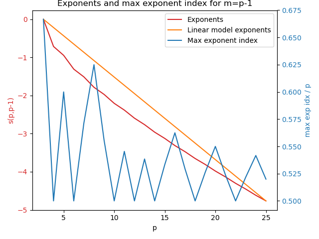
Figure 1: The exponent expressing the size of the highest order coefficient of a Bernstein polynomial written in the Legendre basis as a power of $p$.

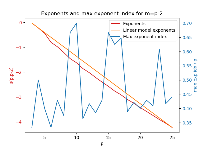
Figure 2: The exponent expressing the size of the second highest order coefficient of a Bernstein polynomial written in the Legendre basis as a power of $m=p$.

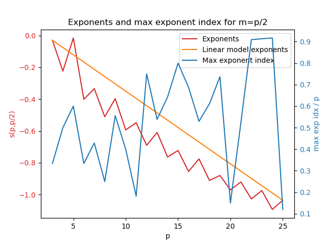
Figure 3: The exponent expressing the size of a middle order coefficient of a Bernstein polynomial written in the Legendre basis as a power of $m=p$.

5 From $[0,h]$ to $[0,\bar{T}]$, the space $\mathcal{P}_{h,p}$

All the above properties are proved for the basis defined on the interval $[0,h]$. Since the goal is to obtain an approximate solution defined on $[0,\bar{T}]$, one can translate the functions $B_{i}(\cdot)$ by $j\cdot h$ for $0\leq j\leq l-1$, in order to obtain the functions

$$B_{i}^{j}(t)=B_{i}(t-jh)=\begin{cases}\frac{\Gamma(p)}{\Gamma(i)\Gamma(p-i+1)}\left(\frac{t-jh}{h}\right)^{i-1}\left(\frac{h+jh-t}{h}\right)^{p-i}\text{ if }t\in I_{j}\\ 0\hphantom{\frac{\Gamma(p)}{\Gamma(i)-}\left(\frac{t}{h}\right)^{i-1}}\text{ otherwise}\end{cases}$$ (60)

where $B_{i}^{0}(t)\equiv B_{i}(t)$. The functions

$$\{B_{i}^{j}(\cdot),1\leq i\leq p,0\leq j\leq l-1\}$$ (61)

form a basis of the piecewise polynomial functions of degree $p$ on $\bar{I}$, with break-points $\{jh\}_{j=1}^{l-1}$. In other words, if $\mathcal{P}_{h,p}$ is the space of such functions, $f\in\mathcal{P}_{h,p}$ if, and only if, there exist $f_{i}^{j}\in\mathbb{R}$ such that

$$f(\cdot)=\sum_{i,j}f_{i}^{j}B_{i}^{j}(\cdot)$$ (62)

It should be noted that the functions in $\mathcal{P}_{h,p}$ are not well defined at break-points, but since the break-points form a set of measure $0$ this is not of concern. The ambiguity in the definition will be lifted rightaway when continuity conditions at break-points are imposed. The dimension of the space $\mathcal{P}_{h,p}$ is equal to $l\cdot p$.

Piecewise polynomial functions are in $H^{1}$ iff they are in $C^{1}$. The SDOF equation being a second order equation, the value of the first derivative is an independent variable. As a consequence, it has to be determined by the choice of functions at break-points and not by the algorithm itself. The space in which the solution should be placed is, therefore,

$$\mathcal{P}_{h,p}^{1}=\mathcal{P}_{h,p}\bigcap C^{1}(I)$$ (63)

A function $f\in\mathcal{P}_{h,p}$ is $C^{1}$ iff the function itself and its first derivative are continuous at break-points. In terms of the coefficients $f_{i}^{j}$, this is equivalent to

$$\begin{array}[]{c@{}l}f_{1}^{j+1}&=f_{p}^{j}\\ f_{2}^{j+1}&=-f_{p-1}^{j}+2f_{p}^{j}\end{array}$$ (64)

The space $\mathcal{P}_{h,p}^{1}$ is consequently of dimension $l\cdot p-2(l-1)$, since it is obtained by imposing $2$ linearly independent conditions on each break-point other than $0$ and $\bar{T}$ on functions in $\mathcal{P}_{h,p}$.

Since the acceleration is a dependent variable, no $C^{2}$ continuity conditions are imposed at break-points. The authors actually tried the version of the algorithm where such conditions were imposed, and the method failed to converge.

6 The first step of the algorithm, $j=0$

In what follows, $p\geq 3$ is an arbitrary natural number, and $l=1$ so that $h=\bar{T}$.

The approximate solution $x_{ap}$ restricted to the interval $[0,h]$ is thus assumed to have the form

$$x_{ap}(\cdot)=\sum_{1\leq i\leq p}u^{0}_{i}B^{0}_{i}(\cdot)=\sum_{1\leq i\leq p}u_{i}B_{i}(\cdot)$$ (65)

where $u_{i}\in\mathbb{R}$ are the $p$ unknown coefficients. The function $v_{0,h}$ bearing the boundary conditions is defined as

$$v_{0,h}=x_{0}B_{1}(\cdot)+x_{h}B_{p}(\cdot)$$ (66)

Since only the first and last functions bear the boundary conditions, we immediately obtain

$$\begin{cases}u_{1}=x_{0}\\ u_{p}=x_{h}\end{cases}$$ (67)

where $x_{h}$ is unknown and treated as a parameter.

Consequently, the approximate solution to the weak problem, $u_{ap}(\cdot)$ assumes the form

$$u_{ap}(\cdot)=\sum_{1<i<p}u_{i}B_{i}(\cdot)$$ (68)

so that

$$x_{ap}(\cdot)=u_{ap}(\cdot)+v_{0,h}(\cdot)$$ (69)

Direct application of the method outlined in §9 of [KK24] gives the $(p-2)\times p$ matrix $[\mathrm{B}]$ with elements

$$\mathrm{B}_{ij}=-\langle\dot{B}_{i}(\cdot),\dot{B}_{j}(\cdot)\rangle_{c}+k\langle B_{i}(\cdot),B_{j}(\cdot)\rangle_{c},2\leq i\leq p-1,1\leq j\leq p$$ (70)

and the $(p-2)$ column vector $\mathrm{F}$ with elements

$$\mathrm{F}_{i}=\langle f(\cdot),B_{i}(\cdot)\rangle_{c}-\langle u_{0}\dot{B}_{1}(\cdot)+u_{p}\dot{B}_{p}(\cdot),\dot{B}_{i}(\cdot)\rangle_{c}+k\langle u_{0}B_{1}(\cdot)+u_{p}B_{p}(\cdot),B_{i}(\cdot)\rangle_{c}$$ (71)

for $2\leq i\leq p-1$, depending on the parameter $u_{p}$.

The linear system

$$[\tilde{\mathrm{B}}].\{u_{i}\}_{i=2}^{p-1}=\{\mathrm{F}\}$$ (72)

where $\tilde{\mathrm{B}}$ is obtained by dropping the first and last columns of matrix $\mathrm{B}$, solves the problem assuming known boundary conditions and thus treating $u_{p}$ as a parameter. Then, the equation

$$\dot{u}(0)=\dot{x}_{0}\iff u_{1}=\frac{h}{p-1}\dot{x}_{0}+x_{0}$$ (73)

allows to solve for $u_{p}$ and determine the rest of the coefficients $u_{i}$.

In total, if one now treats $u_{1}$ and $u_{p}$ as unknown quantities and moves the terms in $\{\mathrm{F}\}$ containing them to the lhs of eq. (72) and considers the full vector of coefficients $\{u_{i}\}_{i=1}^{p}$, they obtain the following linear system

$$[\mathrm{B}\mathrm{B}].\{u_{i}\}_{i=1}^{p}=\{\mathrm{F}\mathrm{F}\}$$ (74)

where the matrix of known coefficients

$$[\mathrm{B}\mathrm{B}]_{p\times p}=\left[\begin{array}[]{c|c}\begin{bmatrix}1&0\\ -\frac{p-1}{h}&\frac{p-1}{h}\end{bmatrix}&[0]_{2\times(p-2)}\\ \hline\cr\{\mathrm{B}^{(1)}\}_{(p-2)\times 2}&[\mathrm{B}^{(2)}]_{(p-2)\times(p-2)}\end{array}\right]$$ (75)

with $\mathrm{B}^{(1)}$ formed by the first two columns of matrix $\mathrm{B}$, and $\mathrm{B}^{(2)}$ by the remaining $p-2$ columns of the same matrix. The rhs vector reads

$$\{\mathrm{F}\mathrm{F}\}_{(p)\times 1}=\begin{Bmatrix}x_{0}\\ \dot{x}_{0}\\ \{\langle f(\cdot),B_{i}(\cdot)\rangle_{c}\}_{i=2}^{p-1}\}\end{Bmatrix}$$ (76)

or, in a more compact form,

$$[\mathrm{B}\mathrm{B}]_{m\times p}=\left[\begin{array}[]{c|c}[C]_{2\times 2}&[0]_{2\times(p-2)}\\ \hline\cr\{\mathrm{B}^{(1)}\}_{(p-2)\times 2}&[\mathrm{B}^{(2)}]_{(p-2)\times(p-2)}\end{array}\right]$$ (77)

where

$$[C]_{2\times 2}=\begin{bmatrix}1&0\\ -\frac{p-1}{h}&\frac{p-1}{h}\end{bmatrix}$$ (78)

The linear system can be efficiently solved in the following way:

1. the first two equations are decoupled from the rest of the system and can be solved separately. They are already in (lower) triangular form.

2. the first column of the vector $\{\mathrm{B}^{(1)}\}_{(p-2)\times 1}$ multiplied by $u_{1}=x_{0}$ and its second column multiplied by $u_{2}$ are subtracted from the vector $\{\langle f(\cdot),B_{i}(\cdot)\rangle_{c}\}_{i=2}^{p-1}\}$ giving the vector $\{\tilde{\mathrm{F}}\}$

3. the rest of the coefficients, $\{u_{i}\}_{i=3}^{p}$, are obtained by

   $$\{u_{i}\}_{i=3}^{p}=[\mathrm{B}^{(2)}]^{-1}.\{\tilde{\mathrm{F}}\}$$ (79)

The first step of the algorithm is completed.

7 The remaining steps

One then can calculate the final displacement

$$x_{ap}(h)=u_{p}$$ (80)

and final velocity

$$\dot{x}_{ap}(h)=\frac{p-1}{h}(u_{p}-u_{p-1})$$ (81)

and iterate the algorithm for the desired number of timesteps in the following way.

For the second step, $j=1$, the approximate solution $x_{ap}$ restricted to the interval $[h,2h]$ and is thus assumed to have the form

$$x_{ap}(\cdot)=\sum_{1\leq i\leq p}u^{1}_{i}B^{1}_{i}(\cdot)=\sum_{1\leq i\leq p}u_{i}^{1}B_{i}(\cdot-h)$$ (82)

The initial displacement and velocity are $x_{ap}(h)$ and $\dot{x}_{ap}(h)$ as calculated here above and the algorithm of the first step applies verbatim. The next steps are carried out in the same fashion.

Remark.

A direct way to parallelize the algorithm using two processors would be the following. The first processor calculates and inverts the matrix $[\mathrm{B}]$, obtaining the matrix $[\mathrm{B}]^{-1}$ that is used throughout the algorithm. The second processor calculates the rhs vector $\{\mathrm{F}\}$, appending the vector corresponding to the timestep $j+1$ at the end of the vector constructed at the end of the $j$-th timestep, and feeds the result to the first processor, which applies the algorithm for each timestep.

There does not seem to be a way to use more processors for this problem. However, piecemeal computation by the second processor of the vector $\{\mathrm{F}\}$ for each timestep $j$, instead of construction of the entire vector of dimension $j*p$ is a direct improvement in terms of memory usage, and should become necessary when treating large-scale MDOF problems.

8 The case $p=3$

The case where $p=3$ is the only case where a direct comparison can be made between the method proposed herein with the traditional step-wise methods, as it is the case of an approximation by a quadradic polynomial. In this case, the matrix $[\mathrm{B}]_{(p-2)\times 3}$ of eq. (70) is a $1\times 3$ vector, and all calculations can be made explicit.

8.1 The undamped case

The expressions when $c>0$, even though still explicit, become cumbersome. The case $c=0$ merits, thus, a separate study for clarity of exposition.

The matrix of eq. (74) reads

$$[\mathrm{B}\mathrm{B}]_{3\times 3}=\left[\begin{array}[]{c|c}\begin{bmatrix}1&0\\ -\frac{2}{h}&\frac{2}{h}\end{bmatrix}&\begin{bmatrix}0\\ 0\end{bmatrix}\\ \hline\cr\{\frac{2}{3h}+\frac{kh}{10},-\frac{4}{3h}+\frac{2kh}{15}\}&[\frac{2}{3h}+\frac{kh}{10}]\end{array}\right]$$ (83)

or, equivalently, already in lower triangular form

$$[\mathrm{B}\mathrm{B}]_{3\times 3}=\begin{bmatrix}1&0&0\\ -\frac{2}{h}&\frac{2}{h}&0\\ \frac{2}{3h}+\frac{kh}{10}&-\frac{4}{3h}+\frac{2kh}{15}&\frac{2}{3h}+\frac{kh}{10}\end{bmatrix}$$ (84)

The rhs vector of the linear system as defined in eq. (76) reads

$$\{\mathrm{F}\mathrm{F}\}_{3\times 1}=\begin{Bmatrix}x_{0}\\ \dot{x}_{0}\\ \langle f(\cdot),B_{2.3,h}(\cdot)\rangle_{0}\end{Bmatrix}$$ (85)

Consequently, the linear system $[\mathrm{B}\mathrm{B}]\{u_{i}\}_{1}^{3}=\{\mathrm{F}\mathrm{F}\}$ admits the unique solution

$$\begin{array}[]{r@{}l}u_{1}&=x_{0}\\ u_{2}&=\frac{h}{2}\dot{x}_{0}+x_{0}\end{array}$$ (86)

which yields

$$u_{3}=\frac{30h\langle f(\cdot),B_{2,3,h}(\cdot)\rangle_{0}+(20-7kh^{2})x_{0}+2(10-kh^{2})h\dot{x}_{0}}{20+3kh^{2}}$$ (87)

This results in the final displacement at time $t=h$, $x_{h}$ being equal to $u_{3}$ as implied by eq. (80), i.e. by

$$x_{h}=\frac{30h\langle f(\cdot),B_{2,3,h}(\cdot)\rangle_{0}+(20-7kh^{2})x_{0}+2(10-kh^{2})h\dot{x}_{0}}{20+3kh^{2}}$$ (88)

The final velocity, $\dot{x}_{h}$, as implied by eq. (81), is given by

$$\dot{x}_{h}=\frac{60\langle f(\cdot),B_{2,3,h}(\cdot)\rangle_{0}-20khx_{0}+(20-7kh^{2})\dot{x}_{0}}{20+3kh^{2}}$$ (89)

Using these formulas, the following theorem can be proved.

Theorem 8.1.

For $c=0$, $k>0$, and $p=3$, the algorithm proposed in §6 boils down to the step-wise iteration of

$$\begin{cases}x_{j+1}=\frac{30h\int_{jh}^{(j+1)h}f(\cdot)B_{2,3,h}(\cdot)+(20-7kh^{2})x_{j}+2(10-kh^{2})h\dot{x}_{j}}{20+3kh^{2}}\\ \dot{x}_{j+1}=\frac{60\int_{jh}^{(j+1)h}f(\cdot)B_{2,3,h}(\cdot)-20khx_{j}+(20-7kh^{2})\dot{x}_{j}}{20+3kh^{2}}\end{cases}$$ (90)

where $x_{0}$ and $\dot{x}_{0}$ are given as initial conditions, and $f$ is the external excitation force.

The approximation rates are as follows:

1. For $f\equiv 0$,

   1. for $x_{j}=1$ and $\dot{x}_{j}=0$,

      $$\begin{array}[]{r@{}l}|x_{j+1}-x_{ex}((j+1)h)|&=O(h^{4})\\ |\dot{x}_{j+1}-\dot{x}_{ex}((j+1)h)|&=O(h^{3})\\ |\mathrm{ME}_{j+1}-\mathrm{ME}_{ex}((j+1)h)|&=O(h^{4})\end{array}$$ (91)

   2. for $x_{j}=0$ and $\dot{x}_{j}=1$,

      $$\begin{array}[]{r@{}l}|x_{j+1}-x_{ex}((j+1)h)|&=O(h^{3})\\ |\dot{x}_{j+1}-\dot{x}_{ex}((j+1)h)|&=O(h^{4})\\ |\mathrm{ME}_{j+1}-\mathrm{ME}_{ex}((j+1)h)|&=O(h^{4})\end{array}$$ (92)

2. For $x_{0}=\dot{x}_{0}=0$ and $f$ piece-wise constant in each interval $[jh,(j+1)h]$:

   $$\begin{array}[]{r@{}l}|x_{j+1}-x_{ex}((j+1)h)|&=O(h^{4})\\ |\dot{x}_{j+1}-\dot{x}_{ex}((j+1)h)|&=O(h^{3})\\ |\mathrm{ME}_{j+1}-\mathrm{ME}_{ex}((j+1)h)|&=O(h^{4})\end{array}$$ (93)

   The constant in the big-O notation is proportional to $f_{j}=f\big{|}_{[jh,(j+1)h]}$.

In the notation of the theorem, $x_{ex}$ represents the exact solution of the corresponding SDOF problem,

$$\mathrm{ME}_{j}=\frac{1}{2}kx_{j}^{2}+\frac{1}{2}\dot{x}_{j}^{2}$$ (94)

is the mechanical energy of the approximate solution, and $\mathrm{ME}_{ex}(jh)$ is the mechanical energy of the exact solution at time $t=jh$.

Proof.

The iteration is just a restatement of the calculations preceding the statement of the theorem.

Regarding the error rates, they follow from the calculation of the Taylor expansions of the iteration formulas for the corresponding cases.

More precisely, the Taylor expansion of the function

$$\frac{20-7t^{2}}{20+3t^{2}}-\cos t$$ (95)

around $t=0$ is

$$\frac{t^{4}}{30}-\frac{71t^{6}}{7200}+O(t^{8})$$ (96)

Similarly, the expansion of

$$\frac{2(10-t^{2})t}{20+3t^{2}}-\sin t$$ (97)

is

$$-\frac{t^{3}}{12}-\frac{7t^{5}}{240}+O(t^{7})$$ (98)

These Taylor expansions account for the good approximation of the displacement in a homogeneous problem, with $0$ excitation force and non-trivial initial conditions (displacement and velocity, respectively).

In the same fashion, the expansion of

$$\frac{-20t}{20+3t^{2}}+\sin t$$ (99)

reads

$$-\frac{t^{3}}{60}-\frac{17t^{5}}{200}+O(t^{7})$$ (100)

which, together with the expansion of eq. (96), accounts for the good approximation of the velocity in the same problem.

Regarding the conservation of Mechanical Energy, the Taylor expansion of

$$\left(\frac{20-7t^{2}}{20+3t^{2}}\right)^{2}+\left(\frac{20t}{20+3t^{2}}\right)^{2}-1$$ (101)

is

$$\frac{t^{4}}{40}-\frac{3t^{6}}{100}+O(t^{8})$$ (102)

while that of

$$\left(\frac{2(10-t^{2})t}{20+3t^{2}}\right)^{2}+\left(\frac{20-7t^{2}}{20+3t^{2}}\right)^{2}-1$$ (103)

is

$$-\frac{t^{4}}{10}+\frac{t^{6}}{25}+O(t^{8})$$ (104)

These approximations establish the good energy-conservation properties of the simplest case of the algorithm proposed herein.

Concerning the terms containing the external force, the following can be obtained by direct calculation. One gets, for $F(t)=\int_{0}^{t}f(t)\mathrm{d}\tau$,

$$\begin{array}[]{r@{}l}\langle f(\cdot),B_{2,3,h}(\cdot)\rangle_{0}&=\int_{0}^{h}f(t)B_{2,3,h}(t)\mathrm{d}t\\ &=-\frac{2}{h}\int_{0}^{h}F(t)\dot{B}_{2,3,h}(t)\mathrm{d}t\\ &=-\frac{2}{h}\int_{0}^{h}F(t)(B_{1,2,h}(t)-B_{2,2,h}(t))\mathrm{d}t\\ &=\frac{2}{h^{2}}\int_{0}^{h}F(t)(2t-1)\mathrm{d}t\end{array}$$ (105)

Since $2t-1$ is the Legendre polynomial of order $1$, this last expression is the projection of $F$ onto linear polynomials, where it is reminded that $F$ is defined modulo a constant. Equivalently, $\langle f(\cdot),B_{2,3,h}(\cdot)\rangle_{0}$ is the projection of $f\in H^{-1}$ onto constants. Replacing $f(\cdot)\equiv 1$ in $\langle f(\cdot),B_{2,3,h}(\cdot)\rangle_{0}$ gives

$$\langle 1,B_{2,3,h}(\cdot)\rangle_{0}=\int_{0}^{h}B_{2,3,h}(t)\mathrm{d}t=\frac{h}{3}$$ (106)

The solution of the undamped SDOF system for $k=1$, homogeneous initial conditions and $f(\cdot)\equiv 1$ reads

$$x(t)=1-\cos t$$ (107)

The Taylor development around $0$ of

$$\frac{10t^{2}}{20+3t^{2}}-(1-\cos t)$$ (108)

reads is

$$-\frac{t^{4}}{30}+\frac{71t^{6}}{7200}+O(t^{8})$$ (109)

which establishes that the method produces a $4$th order approximation under the assumption that the external excitation is constant in $[0,h]$. Concerning the velocity, the force term in eq. (89) for $f(\cdot)\equiv 1$ reads $20h$. This term gives rise to the same Taylor development as in eq. (99), resulting in a $3$rd order approximation for the velocity.

The Taylor development for the Mechanical Energy of the system reads

$$\frac{1}{60}h^{4}-\frac{37}{7200}h^{6}+O(h^{8})$$ (110)

∎

8.2 The damped case

In the case where $c\geq 0$, the matrix of eq. (74) reads

$$[\mathrm{B}\mathrm{B}]_{3\times 3}=\begin{bmatrix}1&0&0\\ -\frac{2}{h}&\frac{2}{h}&0\\ \Xi_{1}&\Xi_{2}&\Xi_{3}\end{bmatrix}$$ (111)

where

$$\begin{array}[]{r@{}l}\Xi_{1}=\Xi_{1}(h,c,k)&=\frac{2}{3h}(2{}_{1}F_{1}(1,4,ch)-{}_{1}F_{1}(2,4,ch))+\frac{kh}{10}{}_{1}F_{1}(2,6,ch)\\ \Xi_{2}=\Xi_{2}(h,c,k)&=-\frac{4}{3h}(2{}_{1}F_{1}(1,4,ch)-{}_{1}F_{1}(2,4,ch)+{}_{1}F_{1}(3,4,ch))\\ &\phantom{\frac{4}{3h}(2{}_{1}F_{1}(1,4,ch)-{}_{1}F_{1}(2,4,ch)}+\frac{2kh}{15}{}_{1}F_{1}(3,6,ch)\\ \Xi_{3}=\Xi_{3}(h,c,k)&=-\frac{2}{3h}({}_{1}F_{1}(2,4,ch)-2{}_{1}F_{1}(3,4,ch))+\frac{kh}{10}{}_{1}F_{1}(4,6,ch)\end{array}$$ (112)

Since ${}_{1}F_{1}(i,p,0)=1$ for all relevant values of $i,p$, one obtains directly the formulas for the undamped case when $c$ is set to $0$.

The rhs vector of the linear system as defined in eq. (76) reads

$$\{\mathrm{F}\mathrm{F}\}_{3\times 1}=\begin{Bmatrix}x_{0}\\ \dot{x}_{0}\\ \int_{0}^{h}e^{ct}f(t)B_{2.3,h}(t)\end{Bmatrix}$$ (113)

This yields the solution

$$\begin{array}[]{r@{}l}u_{1}&=x_{0}\\ u_{2}&=\frac{h}{2}\dot{x}_{0}+x_{0}\\ u_{3}&=\frac{\int_{0}^{h}e^{ct}f(t)B_{2.3,h}(t)-(\Xi_{1}+\Xi_{2})x_{0}-\frac{h}{2}\Xi_{2}\dot{x}_{0}}{\Xi_{3}}\end{array}$$ (114)

Explicit expressions for the quantities $\Xi_{i}$, $i=1,2,3$ can be obtained, but they are cumbersome and not actually useful.

As in the previous paragraph, the displacement and velocity at time $t=h$ can be obtained by the following expressions

$$\begin{array}[]{r@{}l}x_{h}&=\frac{\int_{0}^{h}e^{ct}f(t)B_{2.3,h}(t)-(\Xi_{1}+\Xi_{2})x_{0}-\frac{h}{2}\Xi_{2}\dot{x}_{0}}{\Xi_{3}}\\ \dot{x}_{h}&=\frac{2}{h}\frac{\int_{0}^{h}e^{ct}f(t)B_{2.3,h}(t)-(\Xi_{1}+\Xi_{2}+\Xi_{3})x_{0}-\frac{h}{2}(\Xi_{2}+\Xi_{3})\dot{x}_{0}}{\Xi_{3}}\end{array}$$ (115)

The following theorem can be now be proved.

Theorem 8.2.

For $c\geq 0$, $k>0$, and $p=3$, the algorithm proposed in §6 boils down to the step-wise iteration of

$$\begin{cases}x_{j+1}=\frac{\int_{jh}^{(j+1)h}e^{c\cdot}f(\cdot),B_{2,3}(\cdot)-(\Xi_{1}+\Xi_{2})x_{j}-\frac{h}{2}\Xi_{2}\dot{x}_{j}}{\Xi_{3}}\\ \dot{x}_{j+1}=\frac{2}{h}\frac{\int_{jh}^{(j+1)h}f(\cdot),B_{2,3}(\cdot)-(\Xi_{1}+\Xi_{2}+\Xi_{3})x_{0}-\frac{h}{2}(\Xi_{2}+\Xi_{3})\dot{x}_{0}}{\Xi_{3}}\end{cases}$$ (116)

where $x_{0}$ and $\dot{x}_{0}$ are given as initial conditions, and $f$ is the external excitation force and the $\Xi_{i}$ are defined in eq. (112).

The approximation rates are as follows:

1. For $f\equiv 0$,

   1. for $x_{j}=1$ and $\dot{x}_{j}=0$,

      $$\begin{array}[]{r@{}l}|x_{j+1}-x_{ex}((j+1)h)|&=O(ch^{3})\\ |\dot{x}_{j+1}-\dot{x}_{ex}((j+1)h)|&=O(h^{3})\\ |\mathrm{ME}_{j+1}-\mathrm{ME}_{ex}((j+1)h)|&=O(ch^{3})\\ |\mathrm{ME}^{c}_{j+1}-\mathrm{ME}^{c}_{ex}((j+1)h)|&=O(ch^{3})\end{array}$$ (117)

   2. for $x_{j}=0$ and $\dot{x}_{j}=1$,

      $$\begin{array}[]{r@{}l}|x_{j+1}-x_{ex}((j+1)h)|&=O(h^{3})\\ |\dot{x}_{j+1}-\dot{x}_{ex}((j+1)h)|&=O(ch^{3})\\ |\mathrm{ME}_{j+1}-\mathrm{ME}_{ex}((j+1)h)|&=O(ch^{3})\\ |\mathrm{ME}^{c}_{j+1}-\mathrm{ME}^{c}_{ex}((j+1)h)|&=O(ch^{3})\end{array}$$ (118)

2. For $x_{j}=\dot{x}_{j}=0$ and $f$ piece-wise exponential of the form $f=f_{j}e^{-c\cdot}$ in each interval $[jh,(j+1)h]$, with $f_{j}\in\mathbb{R}$,:

   $$\begin{array}[]{r@{}l}|x_{j+1}-x_{ex}((j+1)h)|&=O(ch^{3})\\ |\dot{x}_{j+1}-\dot{x}_{ex}((j+1)h)|&=O(ch^{3})\\ |\mathrm{ME}_{j+1}-\mathrm{ME}_{ex}((j+1)h)|&=O(h^{4})\\ |\mathrm{ME}^{c}_{j+1}-\mathrm{ME}^{c}_{ex}((j+1)h)|&=O(h^{4})\end{array}$$ (119)

   The constant in the big-O notation depends on $\max|f_{j+1}|$.

where $x_{ex}$ represents the exact solution of the corresponding SDOF problem.

In the notation of the theorem,

$$\mathrm{ME}^{c}_{j}=\frac{1}{2}e^{cjh}kx_{j}^{2}+\frac{1}{2}e^{cjh}\dot{x}_{j}^{2}$$ (120)

is the modified mechanical energy of the approximate solution, and $\mathrm{ME}^{c}_{ex}(jh)$ is the modified mechanical energy of the exact solution at time $t=jh$. The modification is by the exponential factor appearing in the definition of the relevant quantities, see e.g. eq. (70).

Proof.

The iteration is just a restatement of the calculations preceding the statement of the theorem.

Regarding the error rates, they follow from the calculation of the Taylor expansions of the iteration formulas for the corresponding cases. Throughout the proof, $k$ has been set to $1$ for definiteness. The general case follows by rescaling $t$ accordingly. The notation shortcut $\Xi_{i}=\Xi_{i}(t,c,1)$ will be used, while it is reminded that $\omega_{d}=\sqrt{1-(c/2)^{2}}$.

Firstly, consider the homogeneous case, $f\equiv 0$.

More precisely, consider the function

$$-\frac{\Xi_{1}+\Xi_{2}}{\Xi_{3}}-e^{-ct/2}(\cos(\omega_{d}t)+\frac{c}{2\omega_{d}}\sin(\omega_{d}t))$$ (121)

which is equal to the approximate minus the exact solution for $x_{0}=1$ and $\dot{x}_{0}=0$. Its Taylor expansion around $t=0$ is

$$\frac{ct^{3}}{12}+\frac{(4-7c^{2})t^{4}}{120}+O(t^{5})$$ (122)

Similarly, consider the function

$$-\frac{t}{2}\frac{\Xi_{2}}{\Xi_{3}}-e^{-ct/2}\frac{1}{\omega_{d}}\sin(\omega_{d}t)$$ (123)

which is the approximate displacement minus the exact one for $x_{0}=0$ and $\dot{x}_{0}=1$. The expansion of this function reads

$$-\frac{(1-c^{2})t^{3}}{12}+\frac{c(11-7c^{2})t^{4}}{120}+O(t^{5})$$ (124)

These Taylor expansions account for the good approximation of the displacement in a homogeneous problem, with $0$ excitation force and non-trivial initial conditions (displacement and velocity, respectively).

Similarly, consider the function

$$-\frac{2}{t}\frac{\Xi_{1}+\Xi_{2}+\Xi_{3}}{\Xi_{3}}+e^{-ct/2}\frac{1}{\omega_{d}}\sin(\omega_{d}t)$$ (125)

which is the approximate velocity minus the exact one for $x_{0}=1$ and $\dot{x}_{0}=0$. The expansion of this function reads

$$-\frac{(1+2c^{2})t^{3}}{60}-\frac{c(5-4c^{2})t^{4}}{120}+O(t^{5})$$ (126)

Finally, the function

$$-\frac{\Xi_{2}+\Xi_{3}}{\Xi_{3}}-e^{-ct/2}(\cos(\omega_{d}t)-\frac{c}{2\omega_{d}}\sin(\omega_{d}t))$$ (127)

is the approximate velocity minus the exact one for $x_{0}=0$ and $\dot{x}_{0}=1$. The expansion of this function reads

$$\frac{(1-2c^{2})t^{3}}{60}+\frac{(4-9c^{2}+4c^{4})t^{4}}{120}+O(ct^{5})$$ (128)

Regarding the conservation of Mechanical Energy for $x_{0}=1$ and $\dot{x}_{0}=0$, the Taylor expansion of the relevant function (which is too cumbersome to write down) is

$$\frac{ct^{3}}{12}+\frac{(2-c^{2})t^{4}}{40}+O(ct^{5})$$ (129)

while that of the modified Mechanical Energy reads

$$\frac{ct^{3}}{12}+\frac{(6+7c^{2})t^{4}}{120}+O(ct^{5})$$ (130)

Turning to the conservation of Mechanical Energy for $x_{0}=0$ and $\dot{x}_{0}=1$, the Taylor expansion of the relevant function (again, too cumbersome to write down) is

$$\frac{c(1-2c^{2})t^{3}}{60}-\frac{(6+c^{2}-8c^{4})t^{4}}{40}+O(ct^{5})$$ (131)

while that of the modified Mechanical Energy reads

$$\frac{c(1-2c^{2})t^{3}}{60}-\frac{(6-c^{2}-4c^{4})t^{4}}{40}+O(ct^{5})$$ (132)

These approximations establish the good energy-conservation properties of the simplest case of the algorithm proposed here-in in the homogeneous case.

Concerning the terms containing the external force, the following can be obtained by direct calculation. One gets for $F(t)=\int_{0}^{t}e^{ct}f(t)\mathrm{d}\tau$, that $F$, as in the undamped case, is projected onto linear polynomials, resulting in $f$ being of the form $Ke^{-c\cdot}$. Equivalently, $\langle f(\cdot),B_{2,3,h}(\cdot)\rangle_{c}$ is the projection of $f\in H^{-1}$ onto functions of the same form $Ke^{-ct}$. Replacing $f(\cdot)=e^{-c\cdot}$ in $\langle f(\cdot),B_{2,3,h}(\cdot)\rangle_{c}$ gives

$$\langle e^{-c\cdot},B_{2,3,h}(\cdot)\rangle_{c}=\int_{0}^{h}B_{2,3,h}(t)\mathrm{d}t=\frac{h}{3}$$ (133)

i.e. the same result as in the homogeneous case.

The solution of the undamped SDOF system for $k=1$, homogeneous initial conditions and $f(\cdot)=e^{-c\cdot}$ reads

$$x(t)=e^{-ct}-e^{-ct/2}(\cos(\omega_{d}t)-\frac{c}{2\omega_{d}}\sin(\omega_{d}t))$$ (134)

The approximate solution in this case yields

$$u_{3}=\frac{h}{3\Xi_{3}}$$ (135)

The Taylor development around $0$ of the exact minus the approximate value for the displacement reads

$$-\frac{ct^{3}}{6}-\frac{(2-9c^{2})t^{4}}{60}+O(ct^{5})$$ (136)

while for the velocity it reads

$$\frac{(1+3c^{2})t^{4}}{60}+\frac{c(9-8c^{2})t^{4}}{120}+O(t^{5})$$ (137)

Finally, the Taylor development of the difference in the Mechanical Energy reads

$$\frac{(1+3c^{2})t^{4}}{60}+\frac{c(3+14c^{2})t^{5}}{120}+O(t^{6})$$ (138)

while that of the modified Mechanical Energy reads

$$\frac{(1+3c^{2})t^{4}}{60}+\frac{c(1+8c^{2})t^{5}}{120}+O(t^{6})$$ (139)

∎

9 Error estimates

The first step in establishing the estimates for the error of approximation is to obtain relevant density results for the spaces onto which the excitation force is projected.

9.1 Some approximation properties

Firstly, the spaces relevant to approximation, cf. eq.(103) of [KK24], need to be defined in the present context:

$$\begin{array}[]{r@{}l}\mathcal{F}=\mathcal{F}(p,h)&=\mathbb{F}(\mathcal{P})\\ \mathcal{F}_{00}=\mathcal{F}_{00}(p,h)&=\mathbb{F}(\mathcal{P}_{00})\\ \mathcal{F}_{0}^{0}=\mathcal{F}^{0}_{0}(p,h)&=\mathbb{F}(\mathcal{P}^{0}_{0})\\ \mathcal{F}_{ic}&=\mathbb{F}(\mathcal{P}_{ic})\end{array}$$ (140)

where

$$\begin{array}[]{r@{}l}\mathcal{P}=\mathcal{P}(h)&=\mathrm{vec}(\{B_{i}\}_{i=1}^{p})\\ \mathcal{P}_{00}=\mathcal{P}_{00}(h)&=\mathrm{vec}(\{B_{i}\}_{i=3}^{p})\\ \mathcal{P}^{0}_{0}=\mathcal{P}^{0}_{0}(h)&=\mathrm{vec}(\{B_{i}\}_{i=2}^{p-1})\\ \dot{\mathcal{P}}^{0}_{0}=\dot{\mathcal{P}}^{0}_{0}(p,h)&=\{\dot{\varphi},\varphi\in\mathcal{P}^{0}_{0}(p,h)\}\\ &=\{\phi\in\mathcal{P}(p-1,h),\int\phi=0\}\\ \mathcal{P}_{ic}=\mathcal{P}_{ic}(h)&=\mathrm{vec}(\{B_{i}\}_{i=1}^{2})\end{array}$$ (141)

The algorithm proposed herein can be summed up as follows. Let a time-step $h$, a polynomial degree of approximation $p-1\in\mathbb{N}$, $p\geq 3$, and an interval $[0,\bar{T}]$ with $\bar{T}=lh$ with $l\in\mathbb{N}^{*}$ be given. Then, the approximate solution of §9 of [KK24] is constructed in each subinterval $[(j-1)h,jh]$, $1\leq j\leq l$ of length $h$, and the final displacement and velocity at each step $j$ will be used as initial displacement and velocity for the next step. Therefore, in order to obtain convergence one can choose between letting $h\rightarrow 0$, $p\rightarrow\infty$, or eventually both. As a consequence, two types of density results are needed.

From the Stone–Weierstrass approximation theorem (see [Rud76]), the following follows immediately.

Theorem 9.1.

As $p\rightarrow\infty$

$$\begin{array}[]{r@{}l}\mathcal{P}(p,h)&\rightarrow H^{1}([0,h])\\ \dot{\mathcal{P}}^{0}_{0}(p,h)&\rightarrow\{\varphi\in L^{2}_{0}([0,h]),\int\varphi=0\}\end{array}$$ (142)

in the sense of pointwise convergence.

Proof.

The first assertion follows directly from the Stone-Weierstrass theorem, while the second from the fact that $\dot{\mathcal{P}}^{0}_{0}(p,h)$ is the space of polynomials of degree $p-2$ with zero mean value, since they are derivatives of polynomials of degree $p-1$ satisfying homogeneous boundary conditions. ∎

Corollary 9.2.

For any fixed $f\in H^{-1}([0,h])$,

$$\|f-\pi_{\mathcal{P}^{0}_{0}}f\|_{H^{-1}}\rightarrow 0\text{ as }p\rightarrow\infty$$ (143)

9.2 The error rate due to the projection error term

The term $\|f-\pi_{\mathcal{P}^{0}_{0}}f\|_{H^{-1}}$ appears in corollary 9.6 of [KK24], and controls the convergence of the approximation. The following two propositions will allow the estimation of the approximation error. Under the weakest possible assumption that $f\in H^{-1}$, which is the case if $f$ has Dirac-$\delta$ type forces, no rate of convergence can be obtained. Under the relatively week assumption that $F$, an integral of $f$, be $H^{1}$, which covers the case where $f$ Heaviside excitation function, the following results can be proved. Naturally, additional regularity of $f$ improves the rate of convergence of the method.

Proposition 9.3.

Let $e^{c\cdot}f\in H^{s}\rightarrow\mathbb{R}$ be the derivative of $F$, a $H^{s+1}$ function such that $\int_{0}^{h}F=0$, where $s\geq-1$. Then,

$$\|e^{c\cdot}f-\pi_{\mathcal{P}^{0}_{0}}e^{c\cdot}f\|_{H^{-1}}\leq C(p-1)^{-(s+1)}h^{s+1}\|F\|_{H^{s+1}(0,h)}$$ (144)

This proposition provides an estimate for the first term in the estimate of corollary 9.6 of [KK24], the error due to projection onto a finite dimensional subsbpace. This error is bounded by

$$\|e^{c\cdot}f-\pi_{\mathcal{P}^{0}_{0}}e^{c\cdot}f\|_{H^{-1}}=O((p-1)^{-(s+1)}h^{s+1})$$ (145)

for a given excitation function $f$ as $p\rightarrow\infty$ or $h\rightarrow 0$. In the special case where $f$ is $C^{\infty}$ smooth, the rate of convergence is (theoretically) faster than any negative power of the degree of polynomial approximation. Naturally, when the degree is high enough (around $25$ in the experiments carried out be the authors), numerical instabilities appear so this is a purely theoretical result.

Proof.

It follows by application of corollary 3.14 and use of the fact that

$$\|e^{c\cdot}f-\pi_{\mathcal{P}^{0}_{0}}e^{c\cdot}f\|_{H^{-1}(0,h)}=\|F-\pi_{\dot{\mathcal{P}}^{0}_{0}}F\|_{L^{2}_{0}(0,h)}=\|F-T_{p-1}F\|_{L^{2}_{0}(0,h)}$$ (146)

in the notation of corollary 3.14, where the factor $h^{s}$ has been incorporated into the constant $C$, since $h$ is kept constant. ∎

9.3 The error rate due to the misalignment of subspaces

In the following, the error rates due to the angles appearing in the statement of corollary 9.6 of [KK24] are obtained. The case of an undamped system is examined first, since the expressions are much simpler, and the arguments more transparent. In this section, the $L^{2}$ norms of the quantities $F_{i,p,h}$ will be understood as the homogeneous $L^{2}$ norms, equal to

$$\begin{array}[]{r@{}l}\|F_{i,p,h}\|_{L^{2}}^{2}&=\int_{0}^{h}\left(F_{i,p,h}-\frac{1}{h}\int_{0}^{h}F_{i,p,h}\right)^{2}\\ &=\int_{0}^{h}F_{i,p,h}^{2}-\frac{1}{h}\left(\int_{0}^{h}F_{i,p,h}\right)^{2}\end{array}$$ (147)

which is the relevant norm, since the $F_{i,p,h}$ are defined modulo an integration constant.

Since, by time-reparametrization, $k$ can be brought to $k=1$, with $c$ and $h$ transforming according to the rule of eq. (42) of [KK24], $k$ will be suppressed for simplicity and the standing assumption will be $k=1$.

The graphs presented in the following paragraphs are obtained using the data available in this json file. Reference to exact values will be avoided for readability, but the interested reader can access the data, stored in the form of a dictionary.

9.3.1 The undamped system, preliminary calculations

Firstly, concerning the integral of the excitation function in the undamped case when the displacement function is a Bernstein polynomial, the following holds.

Lemma 9.4.

Let $c=0$ and $B_{i,p,h}$, $1\leq i\leq p$, be given. Then, for $F_{i,p,h}=\int\mathbb{F}_{0,k}(B_{i,p,h})$,

$$\begin{array}[]{r@{}l}\int_{0}^{h}F_{i,p,h}^{2}&=\|\dot{B}_{i,p,h}\|_{0}^{2}+k^{2}\|\int B_{i,p,h}\|_{0}^{2}+\frac{2h}{p}kB_{i,p,h}(h)-2k\|B_{i,p,h}\|_{0}^{2}\\ &=\|\dot{B}_{i,p,h}\|_{0}^{2}+k^{2}\|\int B_{i,p,h}\|_{0}^{2}+\frac{2h}{p}k\delta_{i,p}-2k\|B_{i,p,h}\|_{0}^{2}\\ \int F_{i,p,h}&=\delta_{i,p}-\delta_{i,1}+k\frac{h^{2}}{p}\frac{p-i+1}{p+1}\\ \pi_{(\dot{\mathcal{P}}^{0}_{0})^{\perp}}F_{i,p,h}&=k\pi_{(\dot{\mathcal{P}}^{0}_{0})^{\perp}}\int B_{i,p,h}\end{array}$$ (148)

Proof.

The first item follows directly from lemma 4.2 of [KK24] for $c=0$ and an integration by parts.

The second item follows from lemmas 3.2, 3.4 and 3.5.

The third item follows from the same lemma, using the fact that $\dot{B}_{i,p,h}$ has degree $p-2$ just like functions in $\dot{\mathcal{P}}^{0}_{0}$, and functions in $\dot{\mathcal{P}}^{0}_{0}$ are considered modulo their mean value. ∎

The previous lemma has the following corollary, whose proof follows immediately from lem. 3.5, 3.6 and prop. 4.1.

Corollary 9.5.

It holds true that

$$\begin{array}[]{r@{}l}\pi_{(\dot{\mathcal{P}}^{0}_{0})^{\perp}}F_{i,p,h}(\cdot)&=\pi_{(\dot{\mathcal{P}}^{0}_{0})^{\perp}}k\frac{h}{p}\sum\limits_{j=i+1}^{p+1}B_{j,p+1,h}(\cdot)\\ &=k\frac{h}{p}\sum\limits_{m=p-1}^{p}\sqrt{2m+1}\sum\limits_{j=i+1}^{p+1}\Lambda^{-1}_{jm}(p+1)\tilde{L}_{m}(\cdot)\\ &=k\frac{h}{p}\sum\limits_{m=p-1}^{p}\sqrt{2m+1}\tilde{F}_{imp}\tilde{L}_{m}(\cdot)\end{array}$$ (149)

Consequently,

$$\|\pi_{(\dot{\mathcal{P}}^{0}_{0})^{\perp}}F_{i,p,h}\|_{L^{2}}^{2}=k^{2}\frac{h^{2}}{p^{2}}\sum\limits_{m=p-1}^{p}(2m+1)\tilde{F}_{imp}^{2}$$ (150)

The (symmetric, positive-semi-definite) matrix of scalar products

$$\langle\pi_{\dot{\mathcal{P}}^{0}_{0}}F_{i,p,h},\pi_{\dot{\mathcal{P}}^{0}_{0}}F_{j,p,h}\rangle_{0}$$ (151)

is constructed, and its eigenvectors $\{\mathbf{e}_{j}\}_{j=1}^{p}$ calculated. This is the matrix of scalar products of forces appearing in the construction of the approximate solution.

The first two eigenvectors correspond to $0$, or very small, eigenvalues. Linear combinations of these eigenvectors construct the solutions to the homogeneous problem, with $0$ excitation function and non-trivial initial conditions. The first two co-ordinates of the null-eigenvectors are linearly independent, allowing for a solution of the problems

$$\mathbf{A}.\mathbf{\tilde{e}}_{1}=\begin{bmatrix}1\\ 0\end{bmatrix}\text{ and }\mathbf{A}.\mathbf{\tilde{e}}_{2}=\begin{bmatrix}0\\ 1\end{bmatrix}$$ (152)

where

$$\mathbf{A}=\begin{bmatrix}\mathbf{e}_{1,1}&\mathbf{e}_{2,1}\\ \mathbf{e}_{1,2}&\mathbf{e}_{2,2}\end{bmatrix}$$ (153)

Then, following the corresponding part of (74), the eigenvectors $\mathbf{\tilde{e}}_{j},j=1,2$ are expressed in terms of linear combinations of initial conditions resulting in a basis of the nullspace $\mathbf{e}_{disp}$ and $\mathbf{e}_{vel}$ corresponding to the solutions with unit initial displacement and $0$ velocity; and $0$ initial displacement and unit velocity, respectively.

Following the numerical study carried out following prop. 4.1, the equivalent study of the projection of

$$F\in\mathrm{Vec}(\{F_{i,p,h}\}_{i=1}^{i=p})$$ (154)

as in the corollary here above can now be presented.

9.3.2 The undamped system, $h=T$

The study is carried out for $h=T$ in a time-scale at which $k=1.$, i.e. for $h=T=2\pi$ where $T$ is the natural period of the system. The scaling properties with respect to $h$ will be studied afterwards.

It should be noted that in the undamped case the terms coming from the derivatives are in the kernel of the projection operator $\pi_{(\dot{\mathcal{P}}^{0}_{0})^{\perp}}$, while the integrals are not. Their projection on the orthogonal of the kernel, however, remains very small as the study will establish.

The quantity

$$s_{h}=s_{h}(p)=\max_{\max\{|x_{0}|,|\dot{x}_{0}|\}=1}\frac{\log\|\pi_{(\dot{\mathcal{P}}^{0}_{0})^{\perp}}(x_{0}\mathbf{e}_{disp}+\dot{x}_{0}\mathbf{e}_{vel})\|_{L^{2}}}{\log p}$$ (155)

can be calculated, the subscript $h$ standing for ”homogeneous”, so that

$$\|F_{er,h}\|_{L^{2}}=\|\pi_{(\dot{\mathcal{P}}^{0}_{0})^{\perp}}F_{h}\|_{L^{2}}\leq\max\{|x_{0}|,|\dot{x}_{0}|\}p^{s_{h}(p)},\forall F\in\mathrm{Vec}(\{\mathbf{e}_{1},\mathbf{e}_{2}\})$$ (156)

The full signature of the function actually reads $s_{h}(p,h,c,k=1.)$ so that $s_{h}(p)=s_{h}(p,h=T,c=0.)$ for brevity in notation. In other terms, the quantity $K\sin\theta_{h}$ of prop. 9.5 of [KK24] satisfies

$$K\sin\theta_{h}=p^{s_{h}(p)}$$ (157)

The graph in fig. 4 plots an estimate of $s_{h}(p)$. The estimate was obtained by randomly sampling $10000$ initial conditions and keeping the maximum angle over these samples. All null eigenvalues were smaller than $110-2$ (in fact much smaller, but a threshold was set in order to assure smallness).

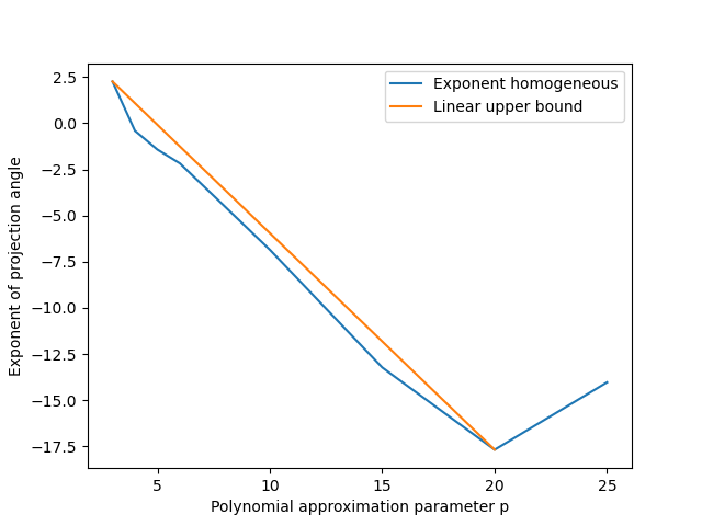
Figure 4: The base-$p$ exponent expressing the error of projection of the force corresponding the homogeneous problem. This is the quantity $s_{h}(p)$ in the established notation.

It can be seen that the point of diminishing returns is reached at around $p=20$, where $K\sin\theta_{h}\approx$110-23$$. For $p=25$ the corresponding value is $2.510-20$. The rise in the exponent is arguably due to numerical instabilities and the diminishing returns point could be pushed further by using more sophisticated numerical analysis machinery. The broken-line model $s^{bl}_{h}(p)$ is given by

$$s^{bl}_{h}(p)=\begin{cases}-1.1725005559764048p+5.771540799001279,0\leq p\leq 20,\\ 0.729932981104102p-32.27712994260885,20\leq p\leq 25,\end{cases}$$ (158)

and it is quite pessimistic in the first leg. In any case, for all relevant values of $p$, $s_{h}(p)\leq s^{bl}_{h}(p)$.

This is the worst-case scenario for the convergence of the algorithm. A range of observed rates of convergence can also be visualized by plotting the exponent of the mean value of the projection angle over the samples, as well as the best-case scenario. The exponent corresponding to the mean value of the angle is denoted by $\bar{s}_{h}(p)$, and the best-case scenario by $\underline{s}_{h}(p)$. They are plotted in fig. 5, where it can be seen that the mean value closely tracks the worst-case exponent.

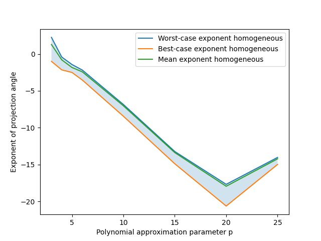
Figure 5: The range of base-$p$ exponents expressing the error of projection of the force corresponding the homogeneous problem. The quantities $s_{h}(p)$, $\bar{s}_{h}(p)$, and $\underline{s}_{h}(p)$ in the established notation are plotted, representing the exponent for the worst-case angle, the mean angle and the best-case angle.

A significant spectral gap separates the two null eigenvectors with the rest of the eigenvectors, whose linear combinations construct the solutions to the non-homogeneous problem, with non-trivial excitation function. Subtraction of the corresponding multiples of $\mathbf{\tilde{e}}_{j},j=1,2$ from $\{\mathbf{e}_{j}\}_{j=3}^{p}$ imposes $0$ initial conditions, and the eigenvectors obtained in this way are denoted by $\{\mathbf{\tilde{e}}_{j}\}_{j=3}^{p}$. It should be noted that $\{\mathbf{\tilde{e}}_{j}\}_{j=1}^{p}$ is still a basis of eignvectors, only not orthogonal. Then, the quantity

$$s_{nh}=s_{nh}(p)=\max_{\begin{subarray}{c}F\in\mathrm{Vec}\{\mathbf{\tilde{e}}_{j}\}_{j=3}^{p}\\ \|F\|_{L^{2}}\leq 1\end{subarray}}\frac{\log\|\pi_{(\dot{\mathcal{P}}^{0}_{0})^{\perp}}F\|_{L^{2}}}{\log p}$$ (159)

can be calculated, so that

$$\|\pi_{(\dot{\mathcal{P}}^{0}_{0})^{\perp}}F\|_{L^{2}}\leq\|F\|_{L^{2}}p^{s_{nh}(p)},\forall F\in\mathrm{Vec}\{\mathbf{\tilde{e}}_{j}\}_{j=3}^{p}$$ (160)

so that the angle $\theta_{nh}$ of prop. 9.5 of [KK24] satisfies

$$\sin\theta_{nh}=p^{s_{h}(p)}$$ (161)

The sine of the angle, instead of the tangent, is calculated for purely practical reasons, as dividing with the hypotenuse is numerically more stable. In the limit $\theta_{nh}\rightarrow 0$, which is the interesting case, the quantities are equal for all practical reasons. For a given approximate solution $x_{ap}$ in $\mathrm{Vec}\{B_{i,p,h}\}_{i=3}^{p}$, the quantity $p^{s_{h}(p)}$ expresses the proportion of the force $\mathbb{F}(x_{ap})$ that contributes to the error term.

The graph in fig. 6 plots an estimate of $s_{nh}(p)$. The estimate was obtained by randomly sampling $10000$ linear combinations of vectors in $\{\mathbf{e}_{j}\}_{j=3}^{p}$ and getting the maximum angle over these samples. The spectral gap condition was that the minimal non-null eigenvalue be at least $1102$ times greater than the biggest null eigenvalue. The spectral gap is actually a lot bigger than $2$ orders of magnitude, but, as before, a threshold was set in order to assure a sufficient spectral gap.

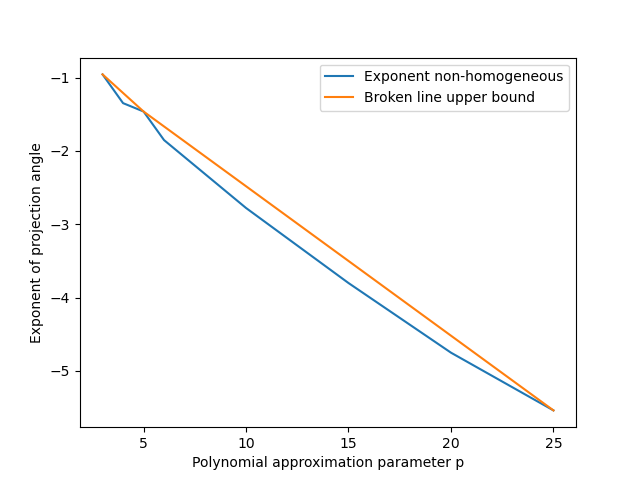
Figure 6: The base-$p$ exponent expressing the error of projection of the force corresponding the homogeneous problem. This is the quantity $s_{h}(p)$ in the established notation.

In the non-homogeneous problem, no point of diminishing returns is observed, which corroborates the hypothesis of not sufficiently strong numerical analysis machinery for treating the null eigenvalues that are (very close to) $0$. The linear model $s^{\ell}_{nh}(p)$ is given by

$$s^{bl}_{nh}(p)=\begin{cases}-0.2530595464212411p-0.19694374410552673,0\leq p\leq 5,\\ -0.20385935288152152p-0.44294471180412476,5\leq p\leq 25,\end{cases}$$ (162)

and it is also a bit pessimistic in the first leg. In any case, for all relevant values of $p$, one still has that $s_{nh}(p)\leq s^{bl}_{nh}(p)$. It can be remarked that, already for $p=3$ the exponent is negative, unlike for the homogeneous problem. However, the factor is merely of the order of $1/3$, not enough to produce an acceptable error rate.

As for the homogeneous problem, the best-case scenario angle and the exponent of the mean angle are plotted in fig. 7, showing that the worst-case scenario tends to be more pessimistic in the homogeneous than in the non-homogeneous case, with the exponent of the mean angle sitting farther than the worst case angle.

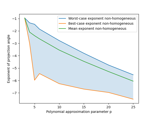
Figure 7: The range of base-$p$ exponents expressing the error of projection of the force corresponding the homogeneous problem. The quantities $s_{nh}(p)$, $\bar{s}_{nh}(p)$, and $\underline{s}_{nh}(p)$ in the established notation are plotted, representing the exponent for the worst-case angle, the mean angle and the best-case angle.

9.3.3 The undamped system, dependence on $h$

In this section, the dependence of the angles of projection on the timestep parameter $h$ will be studied. The scaling of all quantities involved is highly non-trivial, since the derivative scales like $h^{-1}$, the integral like $h$, and the products of derivatives and integrals are constant with respect to $h$.

It should be expected that for small $h$ the dominant term come from the derivative, leading to small angles since $\pi_{(\dot{\mathcal{P}}^{0}_{0})^{\perp}}\dot{B}_{i,p,h}\equiv 0$. For intermediate values of $h$, all terms should contribute roughly in par, while for larger $h$ the integral should start to dominate, leading to greater angles, since integrals are not in the kernel of the projection operator $\pi_{(\dot{\mathcal{P}}^{0}_{0})^{\perp}}$. The products of derivatives and integrals have complicated contribution to the norm of the force, since the derivative can have either sign, while the integrals are always $\geq 0$.

Following eq. (155), the quantity

$$s_{h}=s_{h}(p,h)=\max_{\max\{|x_{0}|,|\dot{x}_{0}|\}=1}\frac{\log\|\pi_{(\dot{\mathcal{P}}^{0}_{0})^{\perp}}(x_{0}\mathbf{e}_{disp}+\dot{x}_{0}\mathbf{e}_{vel})\|_{L^{2}}-s_{h}(p,T)\log p}{\log(h/T)}$$ (163)

can be calculated, so that

$$\|\pi_{(\dot{\mathcal{P}}^{0}_{0})^{\perp}}F\|_{L^{2}}\leq(\max|x_{0}|,|\dot{x}_{0}|)p^{s_{h}(p,T)}\left(\frac{h}{T}\right)^{s_{h}(p,h)},\forall F\in\mathrm{Vec}(\{\mathbf{e}_{1},\mathbf{e}_{2}\})$$ (164)

As for $h=T$, the same number of points are sampled, keeping the worst exponent The same thresholds for null eigenvalues an the spectral gap. Timesteps were sampled in the range from $0.001T$ up to $4T$, i.e. in the range of $0.1\%$ to $400\%$ of the natural period of the system with $k=1$ and $c=0$.

The function $s_{h}(p,h)$ is plotted in figs. 8 and 9 for values of $h<T$ and small, resp. large values of $p$, and in fig. 10 for values of $h>T$ and large values of $p$. The split in $h$ was necessary in order to avoid division by $0$ at $h=T$, and the split in $p$ for clarity.

Figure 8: The base-$h$ exponent expressing the error of projection of the force corresponding the homogeneous problem, for timestep smaller than the natural period and $3\leq p\leq 10$. This is the quantity $s_{h}(p,h)$ in the established notation.

Figure 9: The base-$h$ exponent expressing the error of projection of the force corresponding the homogeneous problem, for timesteps smaller than the natural period, and $10\leq p\leq 25$. This is the quantity $s_{h}(p,h)$ in the established notation.

The graph of fig. 8, featuring values of $p$ in the range $3\leq p\leq 10$, shows a very fast rate of convergence, as all exponents are consistently $>4$, which is an added factor of convergence on top of the factor $p^{s_{h}(p,T)}$, c.f. eq. (164). The graph of fig. 9, featuring $10\leq p\leq 25$, shows a more complicated behavior. While for $p=10,15$ the exponent is positive, leading to a faster convergence, smaller $h$ slows down convergence for $p=20$. The latter remains fast, nonetheless, since, say

$$K\sin\theta_{h}\leq 0.5^{-10}20^{s^{bl}_{h}(20)}\approx$110-20$.$$ (165)

The convergence for $p=25$ is rather indifferent to $h$, if only slightly accelerated by small values of $h$, with exponents in the range $(0,1)$.

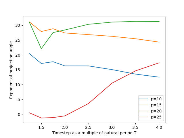
Figure 10: The base-$h$ exponent expressing the error of projection of the force corresponding the homogeneous problem, for timesteps greater than the natural period and $10\leq p\leq 25$. This is the quantity $s_{h}(p,h)$ in the established notation.

The graph of fig. 10 shows equally a non-monotonous behavior of the exponent $s_{h}(p,h)$ for $h>T$. The graph features only high values of $p$, namely $10\leq p\leq 25$, since for low values of $p$ timesteps greater than the natural period $T$ of the system will not produce a small error rate. Already for $p=15$ convergence can remain fast for large values of $h$, since for $h=2T$,

$$K\sin\theta_{h}\leq 2^{-30}15^{s^{bl}_{h}(15)}\approx$110-5$.$$ (166)

Convergence is faster for $p=20$, while the dependence on $h$ gets milder for $p=25$.

Concerning the non-homogeneous problem, following eq. (159), the quantity

$$s_{nh}=s_{nh}(p,h)=\max_{\begin{subarray}{c}F\in\mathrm{Vec}\{\mathbf{\tilde{e}}_{j}\}_{j=3}^{p}\\ \|F\|_{L^{2}}\leq 1\end{subarray}}\frac{\log\|\pi_{(\dot{\mathcal{P}}^{0}_{0})^{\perp}}F\|_{L^{2}}-s_{nh}(p,1)\log p}{\log h}$$ (167)

can be calculated, so that

$$\|\pi_{(\dot{\mathcal{P}}^{0}_{0})^{\perp}}F\|_{L^{2}}\leq\|F\|_{L^{2}}p^{s_{nh}(p,1)}h^{s_{nh}(p,h)},\forall F\in\mathrm{Vec}\{\mathbf{\tilde{e}}_{j}\}_{j=3}^{p}$$ (168)

The function $s_{nh}(p,h)$ is plotted in figs. 11, 12, and 13, with the same parameters as for the homogeneous problem.

Figure 11: The base-$h$ exponent expressing the error of projection of the force corresponding the non-homogeneous problem, for timesteps smaller than the natural period, and $3\leq p\leq 10$. This is the quantity $s_{nh}(p,h)$ in the established notation.

Figure 12: The base-$h$ exponent expressing the error of projection of the force corresponding the non-homogeneous problem, for timesteps smaller than the natural period, and $10\leq p\leq 25$. This is the quantity $s_{nh}(p,h)$ in the established notation.

As show fig. 11, for low-order polynomial approximation and $h$ smaller than $20\%$ of the natural period, the smallness of the timestep contributes to the rate of convergence with an exponent ranging between linear and quadratic, and getting better as $h\rightarrow 0$. As $h$ becomes comparable with the natural period of the system, the corresponding factor never eats too much on the factor produced by $p^{s_{nh}(p)}$, but ceases to contribute.

The same picture holds for higher order polynomial approximation, if only for slightly larger values of $h$, as can be seen in fig. 12. It is reminded that the factor $p^{s_{nh}(p)}$ is, in this case, orders of magnitute smaller, so that the effect of the negative exponent for $h/T$ close to $1^{-}$ is negligible.

Figure 13: The base-$h$ exponent expressing the error of projection of the force corresponding the non-homogeneous problem, for timesteps greater than the natural period and $10\leq p\leq 25$. This is the quantity $s_{nh}(p,h)$ in the established notation.

Moving on to timesteps greater than the natural period of the system, it can be seen in fig. 13 that for $p=10,15$ the factor $h/T$ does contribute to the convergence rate, since the exponent is negative. Convergence becomes practically indifferent to the value of the timestep for $p=20,25$ since the exponent remains negative, but is very close to $0$.

These graphs suggest that mixed approximation schemes, using different degrees of polynomial approximation for the homogeneous and non-homogeneous part, are conceivable, but are outside the scope of the present work.

9.3.4 The damped system, preliminary calculations

Concerning the integral of the excitation function in the damped case when the displacement function is a Bernstein polynomial, the following can be obtained.

Lemma 9.6.

Let $c\geq 0$ and $B_{i,p,h}$, $1\leq i\leq p$, be given. Then, for $F_{i,p,h}=\int e^{c\cdot}\mathbb{F}_{0,k}(B_{i,p,h}(\cdot))$,

$$\begin{array}[]{r@{}l}\int_{0}^{h}F_{i,p,h}^{2}&=\|\dot{B}_{i,p,h}\|_{c}^{2}+k^{2}\|\int B_{i,p,h}\|_{c}^{2}+2k\langle\dot{B}_{i,p,h},\int e^{c\cdot}B_{i,p,h}\rangle_{c}\\ \int F_{i,p,h}&=\int_{0}^{h}e^{c\cdot}\dot{B}_{i,p,h}(\cdot)+k\int_{0}^{h}e^{c\cdot}B_{i,p,h}(\cdot)\\ \pi_{(\dot{\mathcal{P}}^{0}_{0})^{\perp}}F_{i,p,h}&=\pi_{(\dot{\mathcal{P}}^{0}_{0})^{\perp}}e^{c\cdot}\dot{B}_{i,p,h}(\cdot)+k\pi_{(\dot{\mathcal{P}}^{0}_{0})^{\perp}}\int e^{c\cdot}B_{i,p,h}\end{array}$$ (169)

The lemma just states the definitions of the relevant quantities. Closed forms involving the hypergeometric function can be obtained, using lemmas 3.10 and 3.11, and cor. 3.12. They are, however, very cumbersome and not easy to manipulate.

The statement corresponding to cor. 9.5 also becomes difficult to write down. What can be said about the projection is that multiplication by the exponential leaks mass from the derivative into the orthogonal of the kernel of the projection operator $\pi_{(\dot{\mathcal{P}}^{0}_{0})^{\perp}}$, weighed by powers of $ch$.

At the linear level, $e^{ct}=1+ct+O(c^{2}t^{2})$, and this results in

$$\pi_{(\dot{\mathcal{P}}^{0}_{0})^{\perp}}ct\dot{B}_{i,p,h}(t)=c\pi_{(\dot{\mathcal{P}}^{0}_{0})^{\perp}}t\dot{B}_{i,p,h}(t)$$ (170)

being non-trivial, since $t\dot{B}_{i,p,h}(t)$ is of order $p-1$, c.f. also lem. 3.9. In the same way, the presence of the exponential factor leaks more $L^{2}$ mass of the integral $\int e^{c\cdot}B_{i,p,h}$ from the kernel of the projection operator to its orthogonal. In both cases, $L^{2}$ mass is added both in the kernel and its orthogonal, and the trade-off seems impossible to analyze accurately.

The same procedure as in the undamped case can be followed in order to obtain numerical results concerning the matrix of the products of forces.

9.3.5 The effect of damping, $h=T$

The first part of the study is performed by keeping $h=T$, constant, and studying how the curve of 4 changes as damping is switched on. As explained in the previous paragraph, the dependence of the involved quantities on $c$ are very complicated, so, once again the authors are restricted to a numerical study of the phenomenon.

To this end and regarding the homogeneous problem, the quantity of eq. (163) is calculated, taking into account the dependence of $s_{h}=s_{h}(p,c,T)$ on the damping coefficient $c$. The result is plotted in figs. 14, 15, 16, and 17. The graphs are split for $p$ and for $c$ for clarity.

Figure 14: The base-$p$ exponent expressing the error of projection of the force corresponding the homogeneous problem. The graph features low values of $p$, $3\leq p\leq 10$, and low values of $c$, $0\leq c\leq 0.1$. This is the quantity $s_{h}(p,c,T)$ in the established notation.

Figure 15: The base-$p$ exponent expressing the error of projection of the force corresponding the homogeneous problem. The graph features low values of $p$, $3\leq p\leq 10$, and high values of $c$, $0.1\leq c\leq 0.3$. This is the quantity $s_{h}(p,c,T)$ in the established notation.

Figure 16: The base-$p$ exponent expressing the error of projection of the force corresponding the homogeneous problem. The graph features high values of $p$, $10\leq p\leq 25$, and low values of $c$, $0\leq c\leq 0.1$. This is the quantity $s_{h}(p,c,T)$ in the established notation.

Figure 17: The base-$p$ exponent expressing the error of projection of the force corresponding the homogeneous problem. The graph features high values of $p$, $10\leq p\leq 25$, and high values of $c$, $0.1\leq c\leq 0.3$. This is the quantity $s_{h}(p,c,T)$ in the established notation.

The figures show that, in general, the projection angle deteriorates as $c$ grows. As in the undamped case, the part of the graph that is monotonously increasing for $p$ with $c$ held constant can probably be attributed to issues in the numerical calculation of null eigenvectors.

The dominant effect of damping is to increase the mass in the kernel of the projection operator faster than in the orthogonal of the kernel. The effect becomes weaker as $p$ increases, leading to the inverse phenomenon for $p=20$ and small values of $c$ as can be seen in graph 16.

Overall, the introduction of damping slows down the rate of convergence, since for all $p$ it holds that

$$s_{h}(p,0.3,T)\leq s_{h}(p,0,T)+2.55$$ (171)

with the losses being bigger for small $p$.

The corresponding quantity for the non-homogeneous problem, $s_{nh}=s_{nh}(p,c,T)$ is also calculated, as defined in eq. (167), with $c$ switched on. The exponent $s_{nh}=s_{nh}(p,c,T)$ is plotted in figs. 18, 19, 20, and 21, with the same split for $p$ and for $c$, for the sake of clarity.

Figure 18: The base-$p$ exponent expressing the error of projection of the force corresponding the non-homogeneous problem. The graph features low values of $p$, $3\leq p\leq 10$, and low values of $c$, $0\leq c\leq 0.1$. This is the quantity $s_{nh}(p,c,T)$ in the established notation.

Figure 19: The base-$p$ exponent expressing the error of projection of the force corresponding the non-homogeneous problem. The graph features low values of $p$, $3\leq p\leq 10$, and high values of $c$, $0.1\leq c\leq 0.3$. This is the quantity $s_{nh}(p,c,T)$ in the established notation.

Figure 20: The base-$p$ exponent expressing the error of projection of the force corresponding the non-homogeneous problem. The graph features high values of $p$, $10\leq p\leq 25$, and low values of $c$, $0\leq c\leq 0.1$. This is the quantity $s_{nh}(p,c,T)$ in the established notation.

Figure 21: The base-$p$ exponent expressing the error of projection of the force corresponding the non-homogeneous problem. The graph features high values of $p$, $10\leq p\leq 25$, and high values of $c$, $0.1\leq c\leq 0.3$. This is the quantity $s_{nh}(p,c,T)$ in the established notation.

The figures show that the effect of very small damping can be in the direction of increasing the rate of convergence, but the overall tendency is to decrease the rate. For all $p$ it holds that

$$s_{nh}(p,0.3,T)\leq s_{nh}(p,0,T)+1.12$$ (172)

which implies that the approximation of the non-homogeneous problem is less severely affected by the introduction of damping than the homogeneous one.

9.3.6 The effect of damping, dependence on $h$

Finally, the dependence on $h$ is studied, with damping switched on. Once again, the scaling rule for the projection angle seems impossible to analyze with means other than a numerical study.

Thus, the exponent $s_{h}=s_{h}(p,c,h)$ is plotted in the following figures, for a fixed value of $p$ in each one. It is the quantity of eq. (163), which now reads

$$s_{h}=s_{h}(p,c,h)=\max_{\max\{|x_{0}|,|\dot{x}_{0}|\}=1}\frac{\log\|\pi_{(\dot{\mathcal{P}}^{0}_{0})^{\perp}}(x_{0}\mathbf{e}_{disp}+\dot{x}_{0}\mathbf{e}_{vel})\|_{L^{2}}-s_{h}(p,c,T)\log p}{\log(h/T)}$$ (173)

with all relevant parameters being variable, so that

$$\|\pi_{(\dot{\mathcal{P}}^{0}_{0})^{\perp}}F\|_{L^{2}}\leq(\max|x_{0}|,|\dot{x}_{0}|)p^{s_{h}(p,c,1)}h^{s_{h}(p,c,h)},\forall F\in\mathrm{Vec}(\{\mathbf{e}_{1},\mathbf{e}_{2}\})$$ (174)

For $p=3$, the exponent is plotted in fig. 22. Contrary to what was observed for $h=T$, there is a clear monotonicity, with the exponent increasing sharply and steadily as $c$ increases. This effect counteracts sufficiently the loss of convergence due to the deterioration of $s_{h}(p,c,1)$ as $c$ increases, since, for example,

$$3^{s_{h}(3,0,T)}0.1^{s_{h}(3,0,0.1T)}=3^{2.255}0.1^{4.780}=$1.97710-4$$$ (175)

while

$$3^{s_{h}(3,0.3,T)}0.1^{s_{h}(3,0.3,0.1T)}=3^{4.776}0.1^{5.725}=$3.57910-4$$$ (176)

where it is reminded that the value $0.1$ represents the timestep as a fraction of the natural period of the system. The same calculation for $h=0.01T$ yields, respectively, $1.31210-4$ for the undamped system, and $7.67710-4$ for $c=0.3$.

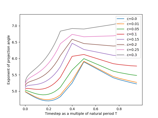
Figure 22: The base-$h$ exponent expressing the error of projection of the force corresponding the homogeneous problem for $p=3$. This is the quantity $s_{h}=s_{h}(3,c,h)$ in the established notation.

The corresponding graph for $p=4$ can be found in fig. 23, where the same phenomenon as for $p=3$ can be observed.

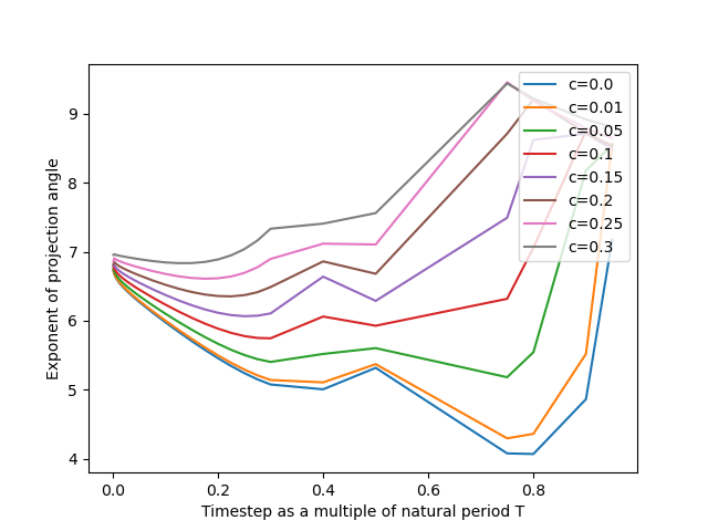
Figure 23: The base-$h$ exponent expressing the error of projection of the force corresponding the homogeneous problem for $p=4$. This is the quantity $s_{h}=s_{h}(4,c,h)$ in the established notation.

The pattern begins to change for higher order approximations, as can be seen in figs. 24 and 25, featuring the curves for $p=5,6$. The monotonic gains are clear for timesteps up to $\approx 25\%$ of the natural period of the system, where a tipping point is reached and monotonicity breaks for stong damping coefficients. The exponent of the timestep remains more favorable, nonetheless, for damped systems relative to the undamped case.

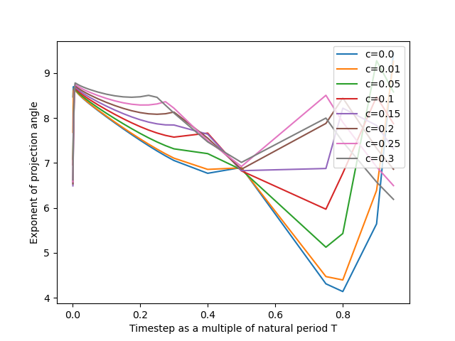
Figure 24: The base-$h$ exponent expressing the error of projection of the force corresponding the homogeneous problem for $p=5$. This is the quantity $s_{h}=s_{h}(5,c,h)$ in the established notation.

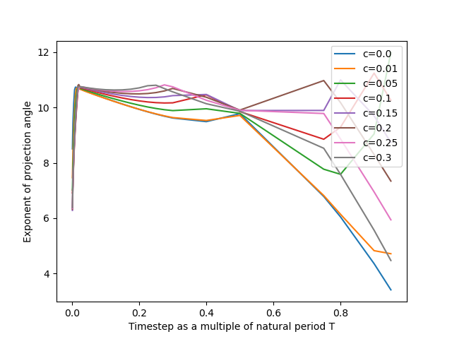
Figure 25: The base-$h$ exponent expressing the error of projection of the force corresponding the homogeneous problem for $p=6$. This is the quantity $s_{h}=s_{h}(6,c,h)$ in the established notation.

Finally, for $p=10$ and timesteps smaller than the natural period the exponent is plotted in fig. 26, while for timesteps ranging from $1.5\times$ up to $4\times T$, in fig. 27.

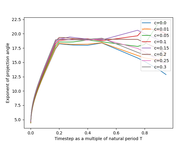
Figure 26: The base-$h$ exponent expressing the error of projection of the force corresponding the homogeneous problem for $p=10$ and timesteps smaller than the natural period of the system. This is the quantity $s_{h}=s_{h}(10,c,h)$ in the established notation.

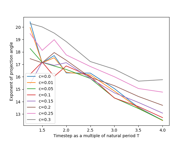
Figure 27: The base-$h$ exponent expressing the error of projection of the force corresponding the homogeneous problem for $p=10$ and timesteps greater than the natural period of the system. This is the quantity $s_{h}=s_{h}(10,c,h)$ in the established notation.

In the case of timesteps smaller than the natural period of the system, damping leads in general to gains in convergence speed, while for timesteps greater than the period the picture is more complicated, as there is no clear monotonicity except for the higher part of the interval of damping coefficients studied.

Turning to the non-homogeneous problem now, the quantity

$$s_{nh}=s_{nh}(p,c,h)=\max_{\begin{subarray}{c}F\in\mathrm{Vec}\{\mathbf{\tilde{e}}_{j}\}_{j=3}^{p}\\ \|F\|_{L^{2}}\leq 1\end{subarray}}\frac{\log\|\pi_{(\dot{\mathcal{P}}^{0}_{0})^{\perp}}F\|_{L^{2}}-s_{nh}(p,c,T)\log p}{\log h}$$ (177)

can be calculated, so that

$$\|\pi_{(\dot{\mathcal{P}}^{0}_{0})^{\perp}}F\|_{L^{2}}\leq\|F\|_{L^{2}}p^{s_{nh}(p,c,T)}h^{s_{nh}(p,c,h)},\forall F\in\mathrm{Vec}\{\mathbf{\tilde{e}}_{j}\}_{j=3}^{p}$$ (178)

As before, the results are presented for fixed $p$, varying $c$ and $h$ in figs. 28, 29, 30, 31.

Figure 28: The base-$h$ exponent expressing the error of projection of the force corresponding the non-homogeneous problem for $p=3$. This is the quantity $s_{nh}=s_{nh}(3,c,h)$ in the established notation.

Figure 29: The base-$h$ exponent expressing the error of projection of the force corresponding the non-homogeneous problem for $p=4$. This is the quantity $s_{nh}=s_{nh}(4,c,h)$ in the established notation.

Figure 30: The base-$h$ exponent expressing the error of projection of the force corresponding the non-homogeneous problem for $p=5$. This is the quantity $s_{nh}=s_{nh}(5,c,h)$ in the established notation.

Figure 31: The base-$h$ exponent expressing the error of projection of the force corresponding the non-homogeneous problem for $p=6$. This is the quantity $s_{nh}=s_{nh}(6,c,h)$ in the established notation.

In this case, the monotonicity is reversed, with convergence speed deteriorating for all relevant values of the timestep. The dependence of $s_{nh}$ on $c$ becomes milder as $c$ increases for all relevant values of $h$. This leads to the following, considerable, deterioration of the convergence rate when passing from $c=0$ to $c=0.3$ for $p=3$ and $h=0.1T$:

$$3^{s_{nh}(3,0,T)}0.1^{s_{nh}(3,0,0.1T)}=3^{-0.9561223833692502}0.1^{1.1565567840705129}=0.02439$$ (179)

while

$$3^{s_{nh}(3,0.3,T)}0.1^{s_{nh}(3,0.3,0.1T)}=3^{-0.6372893192703653}0.1^{0.8230111827097677}=0.07463$$ (180)

For a timestep $h=0.01T$ the quantities read, respectively, $0.0002583$ and $0.005545$.

Finally, for $p=10$ and timesteps smaller than the natural period of the system, fig. 32 shows that in general damping results in a slower congergence rate, which is practically indifferent to $h$ except for small values of $h/T$ and $c$. Fig. 33 shows that in the case of timesteps greater than the natural period, convergence is also practically indifferent to $h$, with all exponents close to $0$.

Figure 32: The base-$h$ exponent expressing the error of projection of the force corresponding the non-homogeneous problem for $p=10$ and timesteps smaller than the natural period of the system. This is the quantity $s_{nh}=s_{nh}(10,c,h)$ in the established notation.

Figure 33: The base-$h$ exponent expressing the error of projection of the force corresponding the non-homogeneous problem for $p=10$ and timesteps greater than the natural period of the system. This is the quantity $s_{nh}=s_{nh}(10,c,h)$ in the established notation.

9.3.7 The aggregate convergence factor

In this final section on the error due to the misalignment of spaces, the aggregate factor is calculated, i.e. the quantity

$$\phi_{\#}(p,c,h)=p^{exp_{\#}(p,c,T)}h^{exp_{\#}(p,c,h)}$$ (181)

for $\#\in\{h,nh\}$. This is necessary due to the convoluted dependence of the exponents on $c$ and $h$, where it is reminded that the dependence on $p$ is the expected one, i.e. decreasing in a practically monotonous way. All graphs are logarithmic in order to accommodate the large range of values of the convergence factor.

In the homogeneous case, $\phi_{h}(p,c,h)$ satisfies

$$\|F_{er}\|_{L^{2}}\leq\phi_{h}(p,c,h)\max\{|x_{0}|,|\dot{x}_{0}|\}$$ (182)

Graphs in figs. 34, 35, 36, 37 and 38, with a varying range of timesteps. Not all damping factors have been retained, for clarity, but it can be seen that monotonicity with respect to $c$ largely holds, with the convergence factor deteriorating as $c$ increases.

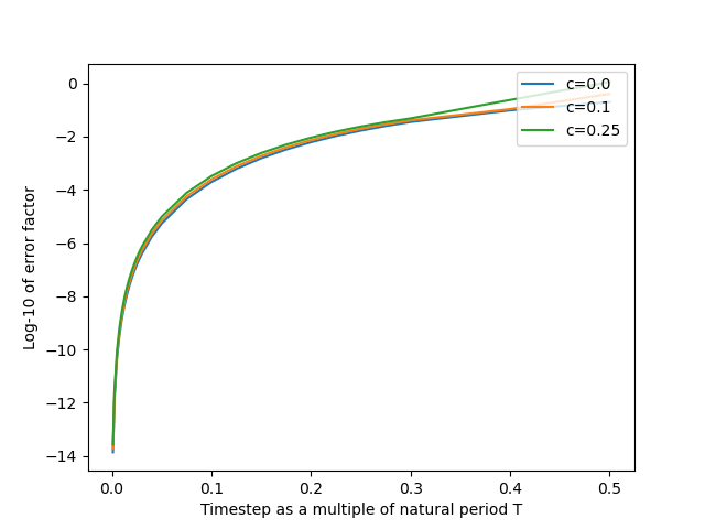
Figure 34: The aggregate factor expressing the error of projection of the force corresponding the homogeneous problem for $p=3$ and timesteps smaller than the natural period of the system. This is the quantity $\phi_{h}(3,c,h)$ in the established notation.

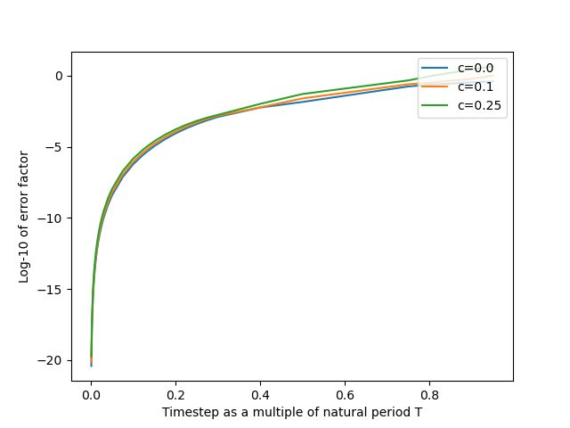
Figure 35: The aggregate factor expressing the error of projection of the force corresponding the homogeneous problem for $p=4$ and timesteps smaller than the natural period of the system. This is the quantity $\phi_{h}(4,c,h)$ in the established notation.

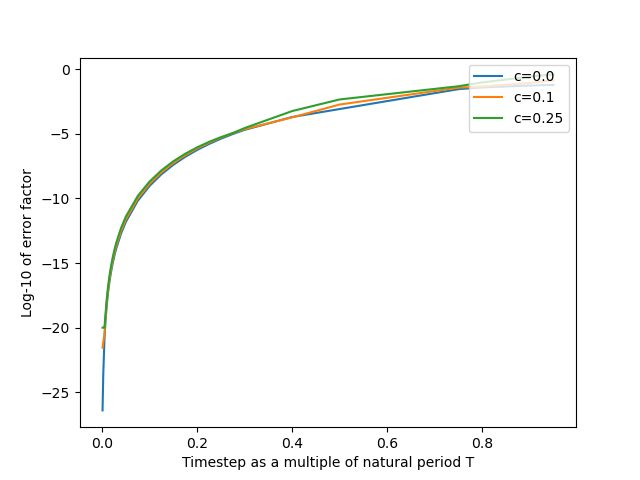
Figure 36: The aggregate factor expressing the error of projection of the force corresponding the homogeneous problem for $p=5$ and timesteps smaller than the natural period of the system. This is the quantity $\phi_{h}(5,c,h)$ in the established notation.

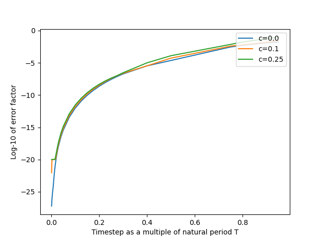
Figure 37: The aggregate factor expressing the error of projection of the force corresponding the homogeneous problem for $p=6$ and timesteps smaller than the natural period of the system. This is the quantity $\phi_{h}(6,c,h)$ in the established notation.

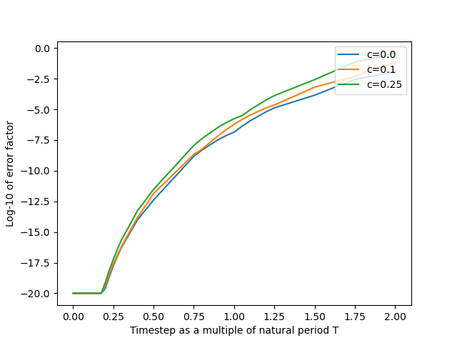
Figure 38: The aggregate factor expressing the error of projection of the force corresponding the homogeneous problem for $p=10$ and timesteps smaller than the natural period of the system. This is the quantity $\phi_{h}(10,c,h)$ in the established notation.

In the non-homogeneous case, $\phi_{nh}(p,c,h)$ satisfies

$$\|F_{er}\|_{L^{2}}\leq\phi_{nh}(p,c,h)\left\|\int e^{c\cdot}\mathbb{F}(x_{ap})\right\|_{L^{2}}$$ (183)

Graphs in figs. 39, 40, 41, 42 and 43. The show monotonicity in $p$ and in $c$, of different directions, and the interesting phenomenon of indifference of the convergence factor on $h$ for big enough values of the timestep.

Figure 39: The aggregate factor expressing the error of projection of the force corresponding the non-homogeneous problem for $p=3$ and timesteps smaller than the natural period of the system. This is the quantity $\phi_{nh}(3,c,h)$ in the established notation.

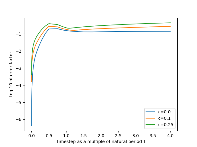
Figure 40: The aggregate factor expressing the error of projection of the force corresponding the non-homogeneous problem for $p=4$ and timesteps smaller than the natural period of the system. This is the quantity $\phi_{nh}(4,c,h)$ in the established notation.

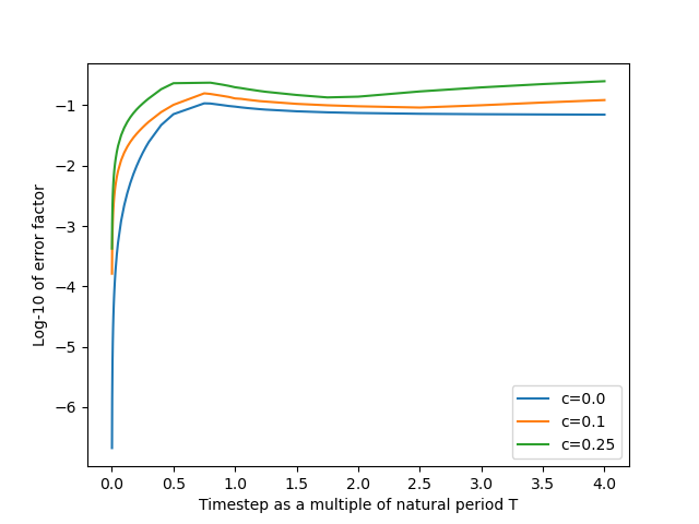
Figure 41: The aggregate factor expressing the error of projection of the force corresponding the non-homogeneous problem for $p=5$ and timesteps smaller than the natural period of the system. This is the quantity $\phi_{nh}(5,c,h)$ in the established notation.

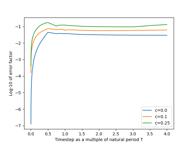
Figure 42: The aggregate factor expressing the error of projection of the force corresponding the non-homogeneous problem for $p=6$ and timesteps smaller than the natural period of the system. This is the quantity $\phi_{nh}(6,c,h)$ in the established notation.

Figure 43: The aggregate factor expressing the error of projection of the force corresponding the non-homogeneous problem for $p=10$ and timesteps smaller than the natural period of the system. This is the quantity $\phi_{nh}(10,c,h)$ in the established notation.

9.4 The error at the end of the timestep

More precise estimates can be be obtained for the error of approximation at time $t=h$, the timestep of the method, both for the homogeneous and the non-homogeneous problem, thanks to the estimates obtained in [KK24], in prop. 9.9 and 9.12 and the calculations in the proof of lem. 4.4, and more precisely eq. (38) and (39). These calculations have as a direct consequence the estimates of propositions 9.9 and 9.12, i.e.

$$\begin{array}[]{r@{}l}|x_{er,h}(h)|&\leq Ke^{-ch/2}\|F_{er,h}(\cdot)\|_{L^{2}_{0}}\left(\|d_{er,h}(\cdot)\|^{2}_{L^{2}_{0}}+\|s_{er,h}(\cdot)\|^{2}_{L^{2}_{0}}\right)^{1/2}\\ |\dot{x}_{er,h}(h)|&\leq e^{-ch/2}\sqrt{h}\|F_{er,h}(\cdot)\|_{L^{2}}+K|x_{er,h}(h)|\end{array}$$ (184)

These expressions are significant because they provide better bounds for the error propagation from one timestep to the next. This is because the final displacement and velocity of one timestep are the initial conditions for the next one, and an error in these initial conditions propagates through the exact solution of the homogeneous SDOF problem.

Proposition 9.7.

The error of approximation for the displacement and the velocity at time $t=h$ satisfy the following estimates

$$\begin{array}[]{r@{}l}|x_{er}(h)|&\leq Ke^{-ch/2}\phi_{h}(p,c,h)\left((p+1)^{-\sigma}h^{\sigma}\|F\|_{H^{\sigma}(0,h)}+\max\{|x_{0}|,|\dot{x}_{0}|\}\phi_{h}(p,c,h)+\|F\|_{L^{2}(0,h)}\phi_{nh}(p,c,h)\right)\\ |\dot{x}_{er}(h)|&\leq e^{-ch/2}\sqrt{h}\left((p+1)^{-\sigma}h^{\sigma}\|F\|_{H^{\sigma}(0,h)}+\max\{|x_{0}|,|\dot{x}_{0}|\}\phi_{h}(p,c,h)+\|F\|_{L^{2}(0,h)}\phi_{nh}(p,c,h)\right)\\ &\phantom{\max\{|x_{0}|,|\dot{x}_{0}|\}\phi_{h}(p,c,h)+\|F\|_{L^{2}(0,h)}\phi_{nh}(p,c,h)}+K|x_{er,h}(h)|\end{array}$$ (185)

In the statement of the proposition, the functions $\phi_{h}$ and $\phi_{nh}$ are defined in eq. (181) and have been studied in §9.3.7.

Proof.

By prop. 9.7 of [KK24], it holds that $\|x\|_{0}\leq K\|F\|_{0}$ if $F$ is the integral of the force corresponding to the SDOF problem with homogeneous initial conditions and $x$ is the solution. Application of this inequality in the case of the force absorbing the initial conditions and the force corresponding to the error of approximation gives

$$\max\{\|d_{er,h}(\cdot)\|_{L^{2}_{0}},\|s_{er,h}(\cdot)\|_{L^{2}_{0}}\}\leq\phi_{h}(p,c,h)$$ (186)

The remaining factors of the estimate on the final displacement are obtained by direct application of the definitions of the related quantities on eq. (184), using cor. 9.6 of [KK24].

Regarding the velocity, eq. (184) yields directly the estimate by substitution of the estimate for the displacement and the estimate for the force used in the estimate of the displacement. ∎

9.5 Error propagation

Proposition 9.7 concludes the error estimates for the algorithm proposed herein. This proposition produces the rate of the propagation of the error, since the final displacement and velocity of timestep $j$ are the initial conditions of timestep $j+1$, and the error is accumulated by the error of approximation of the homogeneous problem. To this error, the error due to the projection of the external force, if the latter is non-zero, is added.

Thus, for initial conditions $x_{0}$ and $\dot{x}_{0}$, and external force $f\in H^{-1}$, the error of displacement at time $t=h$ is given directly by the estimates of prop. 9.7. The errors for times $t\in[0,h]$ is given by prop. 9.9 of [KK24], namely

$$|x_{er}(t)|\leq K\left((p+1)^{-\sigma}h^{\sigma}\|F\|_{H^{\sigma}(0,h)}+\max\{|x_{0}|,|\dot{x}_{0}|\}\phi_{h}(p,c,h)+\|F\|_{L^{2}(0,h)}\phi_{nh}(p,c,h)\right)$$ (187)

while for the velocity, by prop. 9.12

$$\|x_{er}\|_{L^{2}(0,h)}\leq K\left((p+1)^{-\sigma}h^{\sigma}\|F\|_{H^{\sigma}(0,h)}+\max\{|x_{0}|,|\dot{x}_{0}|\}\phi_{h}(p,c,h)+\|F\|_{L^{2}(0,h)}\phi_{nh}(p,c,h)\right)$$ (188)

If $x_{app,1}$, $\dot{x}_{app,1}$ are the displacement and velocity of the approximate solution at time $t=h$, then $|x_{er}(2h)|$ is given by the same formula of prop. 9.7, plus a term

$$\max\{|x_{er}(h)|,|\dot{x}_{er}(h)|\}\phi_{h}(p,c,h)$$ (189)

due to the error propagation, similarly for the velocity.

Higher regularity for $f$ results in $L^{\infty}$ bounds for the velocity as detailed in thm. 9.16 of [KK24], which can be seen by taking one derivative of the equation of motion and applying the same estimates on the velocity instead of the displacement.

10 Conclusions

Even though direct comparison with traditional step-wise methods such as the Newmark method is not easy to make, due to the fundamental difference in the way the methods are built, the advantage of working with the weak formulation and then deriving a numerical method can already be seen in the study of the convergence of the method.

From the estimates it is already clear that, if the order of polynomial approximation is sufficiently high, timesteps comparable to the eigenperiod of the system can potentially give competitive results. This is known to be outside the scope of traditional timestep methods.

Naturally, increasing the order of polynomial approximation comes with additional computational overhead, but on the other hand the number of iterations may become smaller without hindering the precision of the method. The assessment of the trade-off, even though of crucial importance for applications, goes beyond the scope of the present work.

The numerical evidence illustrating the quality of the convergence of the method will be presented in part III of the paper.

References

- [dB78] C. de Boor, A practical guide to splines, Applied Mathematical Sciences 27, Springer-Verlag, New York-Berlin, 1978. MR 507062.
- [CQ82] C. Canuto and A. Quarteroni, Approximation results for orthogonal polynomials in sobolev spaces, Mathematics of Computation 38 (1982), 67–86.
- [Dah56] G. Dahlquist, Convergence and stability in the numerical integration of ordinary differential equations, MATHEMATICA SCANDINAVICA 4 (1956), 33–53. http://dx.doi.org/10.7146/math.scand.a-10454. Available at http://www.mscand.dk/article/view/10454.
- [Far00] R. T. Farouki, Legendre–bernstein basis transformations, Journal of Computational and Applied Mathematics 119 (2000), 145–160. http://dx.doi.org/https://doi.org/10.1016/S0377-0427(00)00376-9. Available at https://www.sciencedirect.com/science/article/pii/S0377042700003769.
- [Kac38] M. Kac, Une remarque sur les polynomes de ms bernstein, Studia Mathematica 7 (1938), 49–51.
- [KK24] N. Karaliolios and D. L. Karabalis, The weak form of the SDOF and MDOF equation of motion, part I: Theory, 2024. arXiv 2407.00441.
- [Rud76] W. Rudin, Principles of mathematical analysis, 3d ed. ed., McGraw-Hill New York, 1976 (English). Available at http://www.loc.gov/catdir/toc/mh031/75017903.html.