A Casimir-like probe for 4D Einstein-Gauss-Bonnet gravity

Abstract

Virtual transitions in a Casimir-like configuration are utilized to probe quantum aspects of the recently proposed four-dimensional Einstein-Gauss-Bonnet (4D EGB) gravity. This study employs a quantum optics-based approach, wherein an Unruh-DeWitt detector (modeled as a two-level atom) follows a radial timelike geodesic, falling freely into an uncharged, nonrotating black hole described by 4D EGB gravity, becoming thermalized in the usual Unruh manner. The black hole, asymptotically Minkowskian, is enclosed by a Casimir boundary proximate to its horizon, serving as a source for accelerated field modes that interact with the infalling detector. Observations are conducted by an asymptotic infinity observer, assuming a Boulware field state. Our numerical analysis reveals that, unlike in Einstein gravity, black holes in 4D EGB gravity can either enhance or suppress the intensity of acceleration radiation, contingent upon the Gauss-Bonnet coupling parameter $\alpha$. Specifically, we observe radiation enhancement for negative $\alpha$ and suppression for positive $\alpha$. These findings offer substantial insights into quantifying the influence of higher-curvature contributions on the behavior of quantum fields in black hole geometries within a 4D spacetime.

I Introduction

Considerable efforts have been made over the past few decades to uncover the deep connection between quantum mechanics, gravity, and thermodynamics Birrell and Davies (1984); Parker and Toms (2009). Among these endeavors, the discovery of Hawking radiation from black holes Hawking (1975) and the Unruh effect for accelerated observers in flat Minkowski spacetime Unruh (1976); Crispino et al. (2008) stand out as pivotal. Another significant phenomenon is Parker’s idea of particle emission due to the expansion of the Universe Parker and Toms (2009). In all these cases, the quantum state of the field is altered by a dynamic background spacetime geometry or the state of motion, resulting in the creation of real particles—an effect arising from the violation of Poincaré invariance Birrell and Davies (1984). This is similar to the dynamical Casimir effect (DCE) Moore (1970); Dodonov (2020), where accelerated plates or boundaries induce the quantum vacuum to radiate particles. Consequently, this scenario fosters a rich intersection of quantum fields, boundaries, and spacetime geometries Scully et al. (2018); Svidzinsky et al. (2018); Lopp et al. (2018); Masood A. S. Bukhari and Wang (2024).

With the advent of precise experimental and observational setups, it has become possible over the decades to test Einstein’s general relativity (GR) in extreme gravity regimes. So far, GR has consistently matched observational data, with milestone achievements including gravitational wave detection Abbott et al. (2016a, b), black hole shadows Akiyama et al. (2019), and neutron star mergers Sänger et al. (2024). However, physicists have long recognized that GR cannot address certain fundamental issues in the Universe, such as the existence of singularities, cosmological acceleration, dark matter, and a consistent merger of quantum mechanics and gravity. Thus, it is evident that a framework beyond GR is needed to resolve these challenges Capozziello and De Laurentis (2011); Berti et al. (2015); Shankaranarayanan and Johnson (2022).
Several alternatives to GR predict additional higher-curvature contributions to the gravitational action. A significant framework within this class of models originates from the works of Lanczos Lanczos (1938) and Lovelock Lovelock (1971, 1972), leading to the well-known Einstein-Gauss-Bonnet (EGB) theory. It has been established that EGB gravity does not introduce modifications to gravitational dynamics unless coupled with additional field degrees of freedom or in spacetime dimensions D$\geq 5$. One example of such additional fields is the dilaton field Blázquez-Salcedo et al. (2016); Konoplya et al. (2020); Maselli et al. (2015); Ayzenberg et al. (2014). In addition to this, EGB gavity theories yield equations of motion that are quadratic in metric tensor. This quadratic nature is a unique feature of EGB gravity among all other alternatives to GR. The interesting coincidence is that the low energy effective descriptions of heterotic string theories also posit quadratic contributions to the dynamics of Einstein gravity Zwiebach (1985); Gross and Witten (1986); Gross and Sloan (1987). It may be noted that the quadratic nature of equations of motion suffice to get rid of Ostrogradsky instability Ostrogradsky (1850) and thus guarantees physicality of the dynamics. Furthermore, EGB gravity theories are characterized by equations of motion that are quadratic in the metric tensor. This quadratic nature distinguishes EGB gravity from other alternatives to GR. An intriguing coincidence arises in that the low-energy effective descriptions of heterotic string theories also incorporate quadratic contributions to the dynamics of Einstein gravity Zwiebach (1985); Gross and Witten (1986); Gross and Sloan (1987). Importantly, the quadratic form of the equations of motion resolves the Ostrogradsky instability Ostrogradsky (1850), ensuring the physical viability of the theory.
Recently, Glavan and Lin Glavan and Lin (2020) addressed the question of Gauss-Bonnet (GB) contributions in 4-dimensional spacetime geometry by proposing a specific rescaling of the GB coupling parameter $\alpha\rightarrow\alpha/\left(\text{D}-4\right)$, where $D$ denotes the spacetime dimensionality. This rescaling ensures a well-defined limit as $D\rightarrow 4$. The resulting model maintains quadratic behavior to prevent Ostrogradsky instability, yet it departs from the implications of the well-known Lovelock theorem Lovelock (1971, 1972); Lanczos (1938). It is noteworthy that no additional field coupling is required in this model. As a new phenomenological competitor to Einstein’s General Relativity (GR), this model has sparked rigorous debates over the years. Some investigations include consistency checks Lu and Pang (2020); Hennigar et al. (2020); Gürses et al. (2020), studies of black hole shadows and quasinormal modes Konoplya and Zinhailo (2020); Kumar and Ghosh (2020); Wei and Liu (2021), analysis of geodesics Guo and Li (2020), particle accelerator models Naveena Kumara et al. (2021), and a wide array of thermodynamic analyses Wei and Liu (2020); Hosseini Mansoori (2021); Eslam Panah et al. (2020); Hegde et al. (2020, 2021); Kumar et al. (2024); Kumar and Ghosh (2023); Ghosh et al. (2020); Masood and Mikki (2024). A comprehensive overview of 4D-EGB gravity, covering its various aspects, can be found in a review article by Fernandes et al. Fernandes et al. (2022).
Recognizing the significance of the findings in Ref. Glavan and Lin (2020), we are driven to investigate the potential quantum radiative signatures of 4D EGB gravity using elements from quantum optics and Casimir physics. Our approach involves a quantum optical cavity positioned with one end near a black hole horizon and the other at asymptotic infinity. Within this setup, a two-level Unruh-DeWitt detector (an atom) falls freely towards the black hole. Virtual transitions arising from the interaction between the detector and the field lead to acceleration radiation, which carries distinct imprints of the underlying gravitational background. Such a setup has been discussed in Ref. Scully et al. (2018), where it was demonstrated that, under appropriate initial conditions, a detector near a Schwarzschild black hole emits radiation with a thermal spectrum. This unique radiative emission, known as Horizon Brightened Acceleration Radiation (HBAR), occurs when the detector is in free fall towards the black hole. This concept has been further explored in various contexts, revealing profound connections between the equivalence principle, quantum optics, and the Hawking-Unruh effect Scully et al. (2018); Fulling and Wilson (2019); Ben-Benjamin et al. (2019); Chatterjee et al. (2021); Sen et al. (2022a). It also underscores connections to the Dynamical Casimir Effect (DCE) and moving mirror models Anderson et al. (2017); Good et al. (2017), frequently employed in studying quantum field behavior in curved spacetimes. But while the original work in Ref. Scully et al. (2018) considers detectors moving along timelike geodesics, subsequent studies have shown that similar phenomena can occur for detectors following null geodesics Chakraborty and Majhi (2019). This novel radiative emission phenomenon can be attributed to the near-horizon physics and conformal quantum mechanics of black holes Camblong et al. (2020); Azizi et al. (2021a, b, c); Sen et al. (2022b, 2023).
Given that quantum field dynamics can elucidate the nature of underlying spacetime geometry Birrell and Davies (1984); Parker and Toms (2009), we view the aforementioned setup as a potential avenue to probe 4D EGB gravity at a deeper level. Through numerical analysis, we demonstrate that 4D EGB gravity can imprint distinct features on the radiation spectrum compared to Einstein’s GR, encompassing both negative and positive values of the Gauss-Bonnet coupling parameter.
The structure of the paper is as follows. The next Sec. II introduces the basics of 4D EGB black hole geometry, accompanied by discussions on the wave equation and the vacuum field state. In Sec. III, we compute the excitation probability or the detector response function of the falling detector. Sec. IV explores possible interpretations of our numerical findings. Finally, conclusions are drawn in Sec. V.

II Conceptual aspects: Our spacetime geometry and the choice of field modes

The static, spherically symmetric metric of an uncharged and nonrotating black hole in 4D EGB gravity is given by Fernandes et al. (2022)

$$ds^{2}=-f(r)\mathrm{d}t^{2}+\frac{1}{f(r)}\mathrm{d}r^{2}+r^{2}(\mathrm{d}\theta^{2}+\sin^{2}\theta\mathrm{d}\phi^{2}),$$ (1)

where

$$f(r)=1+\frac{r^{2}}{2\alpha}\left(1\pm\sqrt{1+\frac{8\alpha M}{r^{3}}}\right),\ \ \$$ (2)

where $\pm$ sign inside brackets denotes Gauss-Bonnet (GB) and GR branches, respectively. Here, we focus solely on the GR branch, as the GB branch is deemed unphysical Fernandes et al. (2022). To determine the event horizon radius, we set

$$f(r)=1+\frac{r^{2}}{2\alpha}\left(1-\sqrt{1+\frac{8\alpha M}{r^{3}}}\right)=0,$$ (3)

which yields

$$r_{\pm}=M^{2}\pm\sqrt{M^{2}-\alpha},$$ (4)

of which the one with plus sign is the real exterior horizon of the black hole. Thus, our event horizon is located at $r_{\rm g}=r_{\pm}=M^{2}+\sqrt{M^{2}-\alpha}$. The parameter $\alpha$ can take both positive and negative values within the range $-32M^{2}\leq\alpha\leq 4M^{2}$, as indicated in Refs. Guo and Li (2020); Konoplya and Zinhailo (2020) (also see Glavan and Lin (2020)). It is evident that a positive GB coupling constant $\alpha$ decreases the black hole horizon radius, whereas a negative $\alpha$ increases it. The limit $\alpha=0$ corresponds to the Schwarzschild black hole in GR. These relationships are illustrated graphically in Fig. 1.

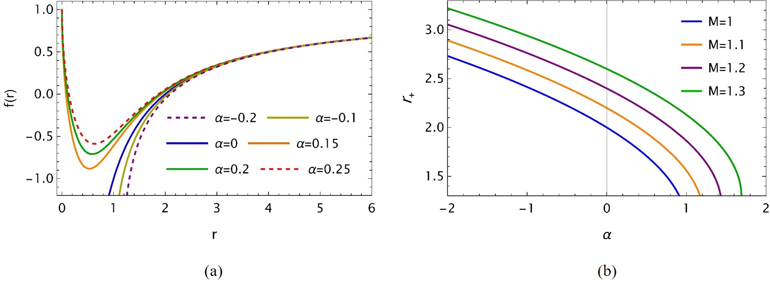
Figure 1: Impact of GB coupling $\alpha$ on (a) $f(r)$ and (b) horizon radius $r_{+}$ to show distinct nature of $\alpha$ for its positive and negative values.

We also note that $r_{+}r_{-}=\alpha$, and as $r\rightarrow 0$, the metric components remain finite. This can be observed from Eq. (2), where $\lim_{r\to 0}f(r)=1$. However, the finiteness of the metric components does not guarantee the absence of singularities due to the fact that the Ricci scalar $R$ and the Kretschmann scalar $R_{\mu\nu\sigma\delta}R^{\mu\nu\sigma\delta}$ vary as $R\propto r^{-3/2}$ and $R_{\mu\nu\sigma\delta}R^{\mu\nu\sigma\delta}\propto r^{-3}$, respectively. It should be noted that for the Schwarzschild case, the Kretschmann scalar near $r=0$ varies as $r^{-6}$, indicating that the GB contribution significantly weakens the singularity by several orders of magnitude Fernandes et al. (2022).

II.1 Detector trajectories

In this section, we analyze the geodesics of the detector to compute both the coordinate time and proper (conformal) time that describe the timelike trajectory of the infalling (massive) detector. Generally, for a given Christoffel connection $\Gamma_{\rho\sigma}^{\mu}$, the complete geodesic equations are expressed as Chandrasekhar (1992)

$$\frac{\mathrm{d}^{2}x^{\mu}}{\mathrm{d}\tau^{2}}+\Gamma_{\rho\sigma}^{\mu}\frac{\mathrm{d}x^{\rho}}{\mathrm{d}\tau}\frac{\mathrm{d}x^{\sigma}}{\mathrm{d}\tau}=0.$$ (5)

Our spacetime geometry of interest exhibits spherical symmetry, and we restrict our analysis to the radial motion of the detector in the equatorial plane. Therefore, we set $\theta=\pi/2$, which implies $\dot{\theta}=0$ and $\dot{\phi}=0$. Consequently, the following conservation equations hold:

$$\Big{(}\frac{\mathrm{d}r}{\mathrm{d}\tau}\Big{)}^{2}=\mathcal{E}^{2}-f(r),\ \ \Big{(}\frac{\mathrm{d}r}{\mathrm{d}t}\Big{)}^{2}=\left[\frac{f(r)}{\mathcal{E}}\right]^{2}\left[\mathcal{E}^{2}-f(r)\right].$$ (6)

Note that $\mathcal{E}$ is a constant representing the specific energy of the detector. It is determined by the initial boundary conditions of the geodesic motion, given by $\mathcal{E}^{2}=f(r)\big{|}_{\text{max}}$. Since we assume that the detector started its motion from asymptotic infinity, where the spacetime is asymptotically Minkowski flat ($r\rightarrow\infty$ implies $f(r)\big{|}_{\text{max}}=1$), these constraints from the above equations lead to

$$\Big{(}\frac{\mathrm{d}r}{\mathrm{d}\tau}\Big{)}^{2}=1-f(r),\ \ \Big{(}\frac{\mathrm{d}r}{\mathrm{d}t}\Big{)}^{2}=f^{2}(r)\left[1-f(r)\right].$$ (7)

It should be emphasized that $\mathcal{E}$, which is related to the maximum of $f(r)$, is the same for both GR and 4D EGB gravity. This value of $\mathcal{E}$ corresponds to asymptotic infinity, where both GR and 4D EGB theories reproduce flat Minkowski geometry.

Now, integrating Eq. (7) along the radial trajectories from some arbitrary initial point $r_{\rm i}$ to a final point $r_{\rm f}$ (where $r_{\rm i}>r_{\rm f}$), we obtain

$$\tau=-\int_{r_{\rm i}}^{r_{\rm f}}\frac{\mathrm{d}r}{\sqrt{1-f(r)}},\ \ t=-\int_{r_{\rm i}}^{r_{\rm f}}\frac{\mathrm{d}r}{f(r)\sqrt{1-f(r)}}.$$ (8)

We now substitute Eq. (2) into Eq. (8) in order to compute $\tau$, resulting in

$$\tau=\frac{2r\sqrt{\sqrt{1+\frac{8\alpha M}{r^{3}}}-1}\tan^{-1}\left(\frac{\sqrt{\sqrt{1+\frac{8\alpha M}{r^{3}}}-1}}{\sqrt{2}}\right)-2\sqrt{2}r}{3\sqrt{\frac{r^{2}\left(\sqrt{1+\frac{8\alpha M}{r^{3}}}-1\right)}{\alpha}}}+\tau_{0}.$$ (9)

Here, $\tau_{0}$ serves as an integration constant, the insignificance of which we establish for the final detector response, as detailed in Sec. III. However, the complexity of the integral for $t$ precludes straightforward analytical computation. Consequently, we resort to numerical methods and present the outcomes in Sec. III. Fig. 2 illustrates the plots of $\tau$ and $t$.

Figure 2: The radial dependence of coordinate time $t$ and proper time $\tau$ illustrates the influence of the Gauss-Bonnet coupling parameter $\alpha$. Panels (a) and (c) depict the proper time for positive and negative $\alpha$, respectively. Similarly, panels (b) and (d) show the coordinate time for positive and negative $\alpha$, respectively.

The plots clearly illustrate that $t$ and $\tau$ exhibit typical Schwarzschild-like behavior. Specifically, $t$, which represents the time measured by an asymptotic observer, diverges as the detector approaches the black hole horizon, located at zero on the rescaled radial coordinate $r-r_{\rm g}$. This divergence signifies that, from the perspective of this observer, the detector never actually crosses the horizon. In contrast, $\tau$ remains finite at the horizon $r-r_{\rm g}$, indicating that from the detector’s own frame of reference, it crosses the horizon in a finite amount of proper time. This disparity highlights the causal structure of black hole horizons and is recognized as gravitational time dilation.

Furthermore, in 4D EGB gravity, the coupling parameter $\alpha$ influences the behavior of $t$ and $\tau$. For positive $\alpha$, which reduces the black hole size as discussed in Sec. II, it takes longer for the detector to approach the horizon as $\alpha$ increases. Conversely, for negative $\alpha$, which inflates the black hole size, the situation is reversed.

II.2 Defining the vacuum state

The response function, or excitation probability, to be calculated in Sec. III, quantifies the detector-field coupling. To achieve this, we must obtain the appropriate field mode by solving the wave equation on the specified spacetime background. Here, we consider the simplest test field: a massless spin-0 Klein-Gordon field, minimally coupled to the spacetime geometry, described by $\nabla_{\mu}\nabla^{\mu}\Phi=0$ Birrell and Davies (1984). Given the spherical symmetry of the spacetime and the presence of a timelike Killing vector $\partial_{t}$, we have $\Phi=\frac{1}{r}Y_{l}(\theta,\phi)\psi(t,r)$, with $Y_{l}$ denoting spherical harmonics and $l$ representing the multipole number. The radial part of the solution, after neglecting the angular dependence $(l=0)$, satisfies the following Schrödinger-like wave equation

$$\Big{(}-\frac{\partial^{2}}{\partial t^{2}}+\frac{\partial^{2}}{\partial r_{*}^{2}}\Big{)}\psi(t,r)=V(r)\psi(t,r).$$ (10)

Here, $r_{*}$ denotes the Regge-Wheeler tortoise coordinate, a useful parameter for describing the propagation of test fields in black hole geometries, defined by Chandrasekhar (1992)

$$r_{*} =\int\frac{\mathrm{d}r}{f(r)}$$ (11)

$$=\int\frac{\mathrm{d}r}{1+\frac{r^{2}}{2\alpha}\left(1-\sqrt{1+\frac{8\alpha M}{r^{3}}}\right)},$$ (12)

where we utilized Eq. (2). Additionally, $V(r)$ represents the effective potential experienced by the field, often describing scattering effects in black hole spacetimes Futterman et al. (2012). However, given our focus on the simplest scenario possible, as also demonstrated in Refs. Scully et al. (2018); Bukhari et al. (2023), $V(r)$ can be neglected. One approach to achieve this is by assuming that the frequency $\nu$ of the field mode is sufficiently large, enabling it to surmount the potential barrier imposed by the spacetime. Consequently, the field mode simplifies to

$$\psi(t,r)=\exp{\left[i\nu(t-r_{*})\right]}.$$ (13)

This represents a normalized outgoing field mode with frequency $\nu$, as observed by an asymptotic infinity observer, qualifying as a Boulware field state. The ingoing field modes generated propagate towards the boundary at the black hole horizon and are lost.
The Boulware field mode described above is an approximate field state obtained by neglecting $V(r)$ and assuming $\nu$ to be very large. This assumption serves as one of the initial conditions required for the existence of HBAR emission Scully et al. (2018). Generally, in the context of black holes, multiple vacuum states are utilized due to the absence of a unique vacuum state in curved spacetime. This leads to various notions of vacuum states, such as the Unruh vacuum, Hartle-Hawking vacuum Birrell and Davies (1984); Parker and Toms (2009), and others. In principle, there should be an infinite number of possible vacuum states due to the violation of Poincaré invariance in curved spacetimes Birrell and Davies (1984). In contrast, for Minkowski space, where the field satisfies Poincaré invariance, the vacuum state remains same for all inertial observers. In our scenario, the choice of the Boulware vacuum state arises because the observations are made by an asymptotic observer, for whom the Boulware field state is most appropriate. In this context, no Hawking radiation is detected by the observer. Moreover, the black hole is assumed to be entirely enclosed by a Casimir boundary, which effectively prevents any potential Hawking quanta from mixing with HBAR flux Scully et al. (2018). This distinction ensures that HBAR emission is fundamentally different from Hawking radiation.
Additionally, we have excluded $l=0$ modes for simplicity. However, considering a smaller $\nu$ such that $V(r)\neq 0$ would lead to the emergence of scattering effects, potentially necessitating the inclusion of greybody factors Sakalli and Kanzi (2022). Nevertheless, we argue that such inclusions would lead to the deviation from the primal essence of HBAR emission, which occurs under specific boundary conditions as emphasized in Refs. Scully et al. (2018); Ben-Benjamin et al. (2019).

III Detector Response

As discussed in the preceding section, the field is in a Boulware vacuum state, ensuring that no Hawking radiation is observed by the asymptotic observer. By neglecting the angular dependence of the field modes, the detector-field interaction Hamiltonian can be expressed as follows Scully et al. (2018):

$$\hat{H}(\tau) =\hbar g\big{[}\hat{a}_{\nu}\psi\left[t(\tau),r(\tau)\right]+\mathrm{H.C.}\big{]}\big{[}\hat{\sigma}(\tau)e^{-i\omega\tau}+\mathrm{H.C.}\big{]}.$$ (14)

Here, $\hat{a}_{\nu}$ is the annihilation operator for the field modes, $\hat{\sigma}$ is the detector lowering operator, and $\mathrm{H.C.}$ denotes the Hermitian conjugate. Here, $g$ is a detector-field coupling parameter indicating the strength of the interaction and can be taken as a constant for a massless Klein-Gordon field (spin-0).

Assuming that the detector is initially in the ground state $|b\rangle$, the probability that it transitions to an excited state $|a\rangle$ with the emission of a field quantum of frequency $\nu$ is given by

$$\Gamma_{\rm exc}=\frac{1}{\hbar^{2}}\bigg{|}\int\mathrm{d}\tau\,\langle 1_{\nu},a|H(\tau)|0,b\rangle\bigg{|}^{2}.$$ (15)

Utilizing time-dependent perturbation theory, such a process is typically prohibited in quantum optics due to energy conservation principles. However, in non-inertial frames influenced by acceleration and gravity, these virtual processes can occur owing to counter-rotating terms in the Hamiltonian Ben-Benjamin et al. (2019), as exemplified by the Unruh effect Unruh (1976). By employing Eq. (14) and performing some additional straightforward computations, Eq. (15) can be reexpressed as

$$\Gamma_{\rm exc} =g^{2}\bigg{|}\int\mathrm{d}\tau\,\psi^{*}(t(\tau),r(\tau))e^{i\omega\tau}\bigg{|}^{2}$$

$$=g^{2}\bigg{|}\int\mathrm{d}r\bigg{(}\frac{\mathrm{d}\tau\,}{\mathrm{d}r}\bigg{)}\psi^{*}(r)e^{i\omega\tau}\bigg{|}^{2}.$$ (16)

Simplifying further, we arrive at

$$\Gamma_{\rm exc} =g^{2}\left|\int\limits_{\infty}^{r_{\rm g}}\mathrm{d}r\,\exp{\left[i\nu\left\{t(r)-r_{*}(r)\right\}\right]}\frac{1}{\sqrt{\frac{r^{2}}{2\alpha}\left(\sqrt{1+\frac{8\alpha M}{r^{3}}}-1\right)}}\exp{\left[i\omega\left\{\frac{2r\sqrt{\sqrt{1+\frac{8\alpha M}{r^{3}}}-1}\tan^{-1}\left(\frac{\sqrt{\sqrt{1+\frac{8\alpha M}{r^{3}}}-1}}{\sqrt{2}}\right)-2\sqrt{2}r}{3\sqrt{\frac{r^{2}\left(\sqrt{1+\frac{8\alpha M}{r^{3}}}-1\right)}{\alpha}}}\right\}\right]}\right|^{2},$$ (17)

which results in a complex expression involving nested integrals with respect to $t(r)$ and $r_{*}$. It’s important to note that the limits of integration correspond to the detector’s trajectory from $r=\infty$ to $r=r_{\rm g}$, the horizon of the black hole. Thus, from Eqs. (8) and (12), we derive:

$$t(r)=-\int_{\infty}^{r_{\rm g}}\frac{\mathrm{d}r\,}{\left[1+\frac{r^{2}}{2\alpha}\left(1-\sqrt{1+\frac{8\alpha M}{r^{3}}}\right)\right]\sqrt{\frac{r^{2}}{2\alpha}\left(\sqrt{1+\frac{8\alpha M}{r^{3}}}-1\right)}},\ \ \ \ r_{*} =\int_{r_{\rm g}}^{\infty}\frac{\mathrm{d}r\,}{1+\frac{r^{2}}{2\alpha}\left(1-\sqrt{1+\frac{8\alpha M}{r^{3}}}\right)}.$$ (18)

Consider now the substitution $r=r_{\rm g}z$, where $\mathrm{d}r=r_{\rm g}\mathrm{d}z$. Using this transformation of variables, we may rewrite $t(r)$ in Eq. (18) as follows:

$$t(z)=-\int_{\infty}^{1}\frac{\mathrm{d}z\,r_{\rm g}}{\left[1+\frac{r_{\rm g}^{2}z^{2}}{2\alpha}\left(1-\sqrt{1+\frac{8\alpha M}{r_{\rm g}^{3}z^{3}}}\right)\right]\sqrt{\frac{r_{\rm g}^{2}z^{2}}{2\alpha}\left(\sqrt{1+\frac{8\alpha M}{r_{\rm g}^{3}z^{3}}}-1\right)}}.$$ (19)

A further substitution of the form $x=z-1$, such that $z=x+1$, yields

$$t(x)=\int_{0}^{\infty}\frac{\mathrm{d}x\,r_{\rm g}}{\left[1+\frac{r_{\rm g}^{2}(x+1)^{2}}{2\alpha}\left(1-\sqrt{1+\frac{8\alpha M}{r_{\rm g}^{3}(x+1)^{3}}}\right)\right]\sqrt{\frac{r_{\rm g}^{2}(x+1)^{2}}{2\alpha}\left(\sqrt{1+\frac{8\alpha M}{r_{\rm g}^{3}(x+1)^{3}}}-1\right)}}.$$ (20)

One can follow a similar calculation for $r_{*}$, arriving at

$$r_{*}(x) =\int_{0}^{\infty}\frac{\mathrm{d}x\,r_{\rm g}}{1+\frac{\left[r_{\rm g}(x+1)\right]^{2}}{2\alpha}\left(1-\sqrt{1+\frac{8\alpha M}{\left[r_{\rm g}(x+1)\right]^{3}}}\right)}.$$ (21)

After deploying all the relevant quantities in Eq. (17), we derive the following final expression for the detector excitation:

$$\Gamma_{\rm exc} =g^{2}r_{\rm g}^{2}\left|\int_{0}^{\infty}\mathrm{d}x\ \ \ \exp{\left[i\nu\left\{t(x)-r_{*}(x)\right\}\right]}\frac{\mathcal{G}}{\sqrt{\frac{(r_{\rm g}[x+1])^{2}}{2\alpha}\left(\sqrt{1+\frac{8\alpha M}{(r_{\rm g}\left[x+1\right])^{3}}}-1\right)}}\right|^{2},$$

where

$$\mathcal{G}=\exp{\left[i\omega\left\{\frac{2r_{\rm g}\left(x+1\right)\sqrt{\sqrt{1+\frac{8\alpha M}{(r_{\rm g}\left[x+1\right])^{3}}}-1}\tan^{-1}\left(\frac{\sqrt{\sqrt{1+\frac{8\alpha M}{(r_{\rm g}\left[x+1\right])^{3}}}-1}}{\sqrt{2}}\right)-2\sqrt{2}\left[r_{\rm g}(x+1)\right]}{3\sqrt{\frac{(r_{\rm g}\left[x+1\right])^{2}\left(\sqrt{1+\frac{8\alpha M}{(r_{\rm g}\left[x+1\right])^{3}}}-1\right)}{\alpha}}}\right\}\right]}.$$ (22)

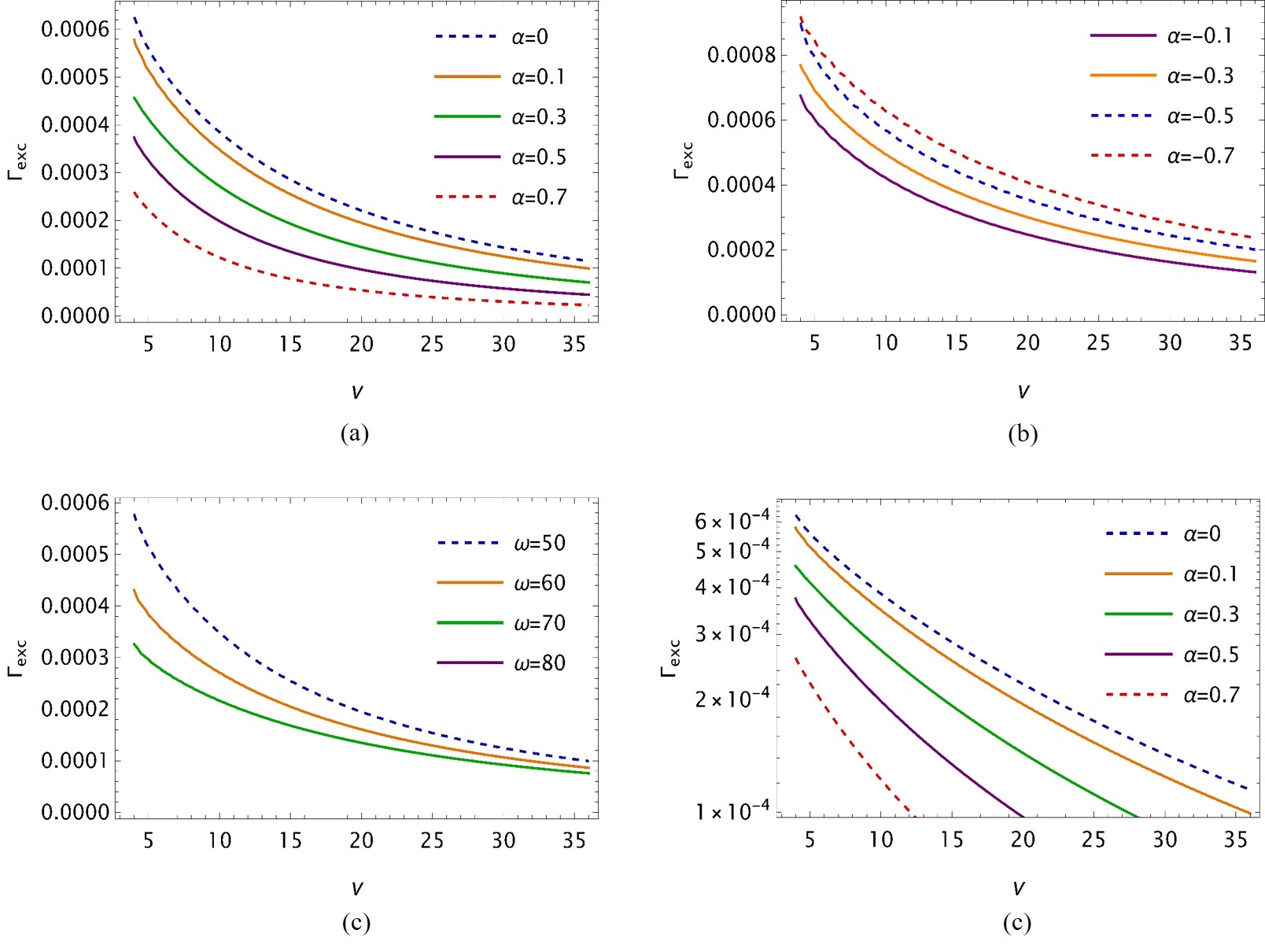
Figure 3: Impact of Gauss-Bonnet coupling $\alpha$ on detector response $\Gamma_{exc}$:(a) positive $\alpha$, and (b) negative $\alpha$, for a fixed black hole mass $M$.(c) indicates impact of detector transition frequency $\omega$, and (d) is the log-log plot of $\Gamma_{\rm exc}$ to emphasize the BE-type nature of the spectrum. We chose $M=1$, $\omega=50$ and $g=1$.

This represents the primary outcome of our investigation. The numerical integral in (22) is notably intricate, demanding a careful approach for its accurate computation. To achieve that, in what follows we deploy the numerical integration capabilities of the Mathematica symbolic math package for performing all required calculations. The figures presented in Fig. 3 were generated using optimized settings.

IV Results and discussions

Based on the preceding analysis, the two-level Unruh-DeWitt detector, operating in the Boulware vacuum state, registers detections while in free fall (inertial). This observation appears to challenge established field-theoretic concepts associated with the Hawking-Unruh effect. Specifically, there is no emission of Hawking radiation in the Boulware state as observed from asymptotic infinity, nor does the Unruh effect manifest for inertial detectors in the Minkowski vacuum. However, HBAR emission from detectors operates on different principles Scully et al. (2018); Ben-Benjamin et al. (2019). While it shares similarities with Hawking radiation, such as the thermal nature of the emitted flux and the associated Bekenstein-Hawking entropy-area correspondence, there are also distinct characteristics. Notably, HBAR emission involves the evolution of field modes in pure states and includes phase correlations between them. These aspects naturally relate to the black hole information paradox Hawking (1976); Almheiri et al. (2021).
In Fig. 3, we present the detector excitation probability, $\Gamma_{\rm exc}$, plotted as a function of the emitted radiation frequency, $\nu$. The impact of the GB coupling parameter, $\alpha$, is depicted in Figs. 3(a) and 3(b) for positive and negative values of $\alpha$, respectively. Fig. 3(c) illustrates how the detector transition frequency, $\omega$, influences $\Gamma_{\rm exc}$, while Fig. 3(d), shown on a log-log scale, highlights the behavior of $\Gamma_{\rm exc}$ near the origin and its convergence at higher frequencies. It is important to note that our interpretations and analyses are based on numerical estimations detailed in the preceding sections. These figures provide a comprehensive view of the radiative characteristics under consideration, elucidating the role of $\alpha$ and the detector’s transition frequency in shaping $\Gamma_{\rm exc}$.
From all plots, one of the prominent features observed is the thermal nature of the HBAR radiation flux, characterized by a Bose-Einstein (BE) distribution. This observation leads us to conclude that $4$D Einstein-Gauss-Bonnet (EGB) gravity does not alter the thermal nature of the flux, consistent with earlier findings Scully et al. (2018); Ben-Benjamin et al. (2019); Chakraborty and Majhi (2019); Azizi et al. (2021b, c) in the context of Einstein gravity. This characteristic mirrors the thermal emission observed in Hawking radiation from pure black holes with asymptotically flat geometries. It is noteworthy that for the so-called “dirty” black holes beyond the Kerr-Newman family, such as in the de Sitter case, there exists the possibility of observing a nonthermal spectrum Kastor and Traschen (1996); Visser (2015); Qiu and Traschen (2020); Bukhari et al. (2023). The detector excitation probability $\Gamma_{\rm exc}$, as observed in Fig. 3(a), decreases with increasing positive values of $\alpha$ and increases with negative values of $\alpha$. As previously discussed, positive $\alpha$ reduces the size of the black hole horizon [see Fig. 1(b)], leading to the conclusion that smaller black holes emit less radiation flux compared to larger ones. This reasoning can similarly be applied to negative values of $\alpha$. It is crucial to emphasize that in the limit $\alpha\rightarrow 0$, depicted in Fig. 3(a), the scenario converges to that of the pure Schwarzschild black hole.
The attenuation and augmentation of particle production can be conceptually grasped as follows. Particles generated within black hole spacetimes, as in Hawking radiation, experience backreaction due to the gravitational tidal forces exerted by the black hole. This backreaction diminishes the intensity of the radiation. Tidal effects in black holes stem from their surface gravities, which are directly related to their horizon radii. Specifically, for a black hole with a horizon radius $r_{g}$, the surface gravity varies inversely with the square of $r_{g}$. This relationship implies that larger black holes have smaller surface gravities and correspondingly weaker tidal effects, and conversely, smaller black holes exhibit stronger tidal effects.
In the context of positive $\alpha$, the black hole horizon size decreases monotonically, leading to stronger surface gravity and tidal effects compared to a Schwarzschild black hole ($\alpha=0$). Consequently, particles generated within such spacetimes experience heightened backreaction, impeding their propagation. This results in fewer particles escaping to asymptotic infinity, thereby reducing the intensity of the particle spectrum, as illustrated in Fig. 3(a). Conversely, for negative values of $\alpha$, the black hole horizon radius increases, indicating reduced backreaction and tidal forces. This condition allows more particles to escape from the black hole spacetime, leading to an enhancement in the radiation flux, as depicted in Fig. 3(b). This constitutes the primary finding of our study, distinguishing $4$D EGB gravity from Einstein GR.
To investigate the influence of the detector transition frequency $\omega$ on the radiation intensity, we plot $\Gamma_{\rm exc}$ against $\omega$ in Fig. 3(c). The graphs clearly demonstrate a decrease in radiation intensity as $\omega$ increases. This behavior aligns with the principles of the Unruh effect Unruh (1976) and can be understood in terms of energy conservation: higher detector transition frequencies require more energy to excite the detector, resulting in a lower excitation probability, and vice versa.
Furthermore, to gain insight into the spectrum’s behavior at low and high frequencies ($\nu$), we reexamined $\Gamma_{\rm exc}$ from Fig. 3(a) using a log-log scale. It is evident that the spectrum exhibits a finite Bose-Einstein (BE)-type distribution near the origin where $\nu\rightarrow 0$. As $\nu$ increases, the spectrum converges and exhibits a thermal tail, characteristic of a BE or Planckian distribution.
In the meantime, it is pertinent to consider the testable implications of this study. We can draw insights from analog gravity systems Barcelo et al. (2005); Braunstein et al. (2023); Jacquet et al. (2020), which have been actively utilized over the last few decades to explore quantum field-theoretic phenomena in curved spacetimes. These systems have provided valuable analogs for understanding effects such as Hawking radiation Weinfurtner et al. (2011), the Unruh effect Hu et al. (2019), and Parker particle generation in expanding spacetimes Steinhauer et al. (2022). Most of these setups, whether based on condensed matter or quantum optical systems, are closely tied to Casimir physics involving moving boundaries. This connection is particularly relevant to our study, which is largely inspired by these concepts. Recently, condensed matter systems have been utilized to explore phenomena extending beyond particle generation in exotic backgrounds, including applications to fluid/gravity correspondence Hubeny et al. (2012). Looking forward, there is potential for future tabletop experiments to simulate black hole horizons resembling those in $4$D EGB gravity Glavan and Lin (2020) or to investigate HBAR radiation scenarios Scully et al. (2018), where our findings could offer valuable insights.

V Conclusion and outlook

The exploration of theories beyond Einstein gravity has evolved in parallel with general relativity (GR) itself. These modified or extended gravity theories aim to tackle fundamental cosmological issues such as cosmic acceleration, singularities, and dark matter. Among these models, Einstein-Gauss-Bonnet (EGB) gravity stands out, predicting higher-curvature corrections to the Einstein-Hilbert action. These corrections arise either in higher dimensions or through additional field couplings to the gravitational action. Interestingly, these contributions also emerge in the low-energy effective description of heterotic string theory. The 4D EGB theory represents a novel gravitational model that has sparked intense debate since its inception several years ago. This model predicts the presence of a Gauss-Bonnet (GB) term within 4D spacetime, which would otherwise not contribute to the latter’s geometry. Its ability to provide a nontrivial contribution is achieved through a redefinition (rescalling) of the GB parameter Glavan and Lin (2020). Importantly, this theory circumvents the Lovelock theorem and sidesteps Ostrogadsky instability, ensuring that the resulting gravitational dynamics remain quadratic. The theory has been scrutinized across various phenomenological fronts.
In this paper, we examined the quantum radiative properties of a nonrotating, uncharged black hole in $4$D Einstein-Gauss-Bonnet (EGB) gravity using a Casimir-type configuration. The black hole, surrounded by a reflecting mirror, induced accelerated field modes from the Boulware vacuum state. We analyzed the interaction of these field modes with a freely falling two-level Unruh-DeWitt detector, which exhibited characteristic clicking behavior akin to the Unruh effect.
The spectrum detected by the detector follows a Bose-Einstein (BE) distribution, with a notable dependence on the GB parameter $\alpha$. By examining both positive and negative values of $\alpha$, we studied their influence on the radiation intensity emitted by the detector. We observed that radiation intensity diminishes when $\alpha$ is positive. This reduction is attributed to the shrinking of the black hole size caused by positive $\alpha$. Conversely, for negative $\alpha$, we observed an increase in radiation intensity. The reduction or augmentation of the radiation flux is examined in relation to a pure Schwarzschild black hole, where the limit $\alpha\rightarrow 0$ is considered. Additionally, we observed that the transition frequency of the detector reduces the profile of particle creation due to the high energy needed for its excitation, consistent with the standard predictions of the Unruh effect. Finally, the spectrum is finite near the origin and monotonically converges at the high end of the frequency ranges, yielding the distinctive thermal tail characteristic of a Bose-Einstein or Planckian distribution.
Our work provides an opportunity to explore various aspects of 4D EGB gravity by incorporating different energy-matter distributions around the simplest black hole model possible. Moreover, exploring other types of detector-field couplings could yield valuable insights into the nature of field configurations within the context of 4D EGB gravity. These and similar questions constitute promising extensions of this work, which we plan to pursue in the future.

References

- Birrell and Davies (1984) N. D. Birrell and P. C. W. Davies, Quantum Fields in Curved Space, Cambridge Monographs on Mathematical Physics (Cambridge Univ. Press, Cambridge, UK, 1984).
- Parker and Toms (2009) L. E. Parker and D. J. Toms, Quantum Field Theory in Curved Spacetime: Quantized Fields and Gravity (Cambridge University Press, Cambridge, England, 2009).
- Hawking (1975) S. W. Hawking, Commun. Math. Phys. 43, 199 (1975).
- Unruh (1976) W. G. Unruh, Phys. Rev. D 14, 870 (1976).
- Crispino et al. (2008) L. C. B. Crispino, A. Higuchi, and G. E. A. Matsas, Rev. Mod. Phys. 80, 787 (2008).
- Moore (1970) G. T. Moore, Journal of Mathematical Physics 11, 2679 (1970).
- Dodonov (2020) V. V. Dodonov, MDPI Physics 2, 67 (2020).
- Scully et al. (2018) M. O. Scully, S. Fulling, D. Lee, D. N. Page, W. Schleich, and A. Svidzinsky, Proc. Nat. Acad. Sci. 115, 8131 (2018), arXiv:1709.00481 [quant-ph] .
- Svidzinsky et al. (2018) A. A. Svidzinsky, J. S. Ben-Benjamin, S. A. Fulling, and D. N. Page, Phys. Rev. Lett. 121, 071301 (2018).
- Lopp et al. (2018) R. Lopp, E. Martin-Martinez, and D. N. Page, Class. Quant. Grav. 35, 224001 (2018), arXiv:1806.10158 [quant-ph] .
- Masood A. S. Bukhari and Wang (2024) S. Masood A. S. Bukhari and L.-G. Wang, Front. Phys. (Beijing) 19, 54203 (2024), arXiv:2307.12222 [gr-qc] .
- Abbott et al. (2016a) B. P. Abbott et al. (LIGO Scientific, Virgo), Phys. Rev. Lett. 116, 061102 (2016a), arXiv:1602.03837 [gr-qc] .
- Abbott et al. (2016b) B. P. Abbott et al. (LIGO Scientific, Virgo), Phys. Rev. Lett. 116, 221101 (2016b), [Erratum: Phys.Rev.Lett. 121, 129902 (2018)], arXiv:1602.03841 [gr-qc] .
- Akiyama et al. (2019) K. Akiyama et al. (Event Horizon Telescope), Astrophys. J. Lett. 875, L1 (2019), arXiv:1906.11238 [astro-ph.GA] .
- Sänger et al. (2024) E. M. Sänger et al., (2024), arXiv:2406.03568 [gr-qc] .
- Capozziello and De Laurentis (2011) S. Capozziello and M. De Laurentis, Phys. Rept. 509, 167 (2011), arXiv:1108.6266 [gr-qc] .
- Berti et al. (2015) E. Berti et al., Class. Quant. Grav. 32, 243001 (2015), arXiv:1501.07274 [gr-qc] .
- Shankaranarayanan and Johnson (2022) S. Shankaranarayanan and J. P. Johnson, Gen. Rel. Grav. 54, 44 (2022), arXiv:2204.06533 [gr-qc] .
- Lanczos (1938) C. Lanczos, Annals Math. 39, 842 (1938).
- Lovelock (1971) D. Lovelock, J. Math. Phys. 12, 498 (1971).
- Lovelock (1972) D. Lovelock, J. Math. Phys. 13, 874 (1972).
- Blázquez-Salcedo et al. (2016) J. L. Blázquez-Salcedo, C. F. B. Macedo, V. Cardoso, V. Ferrari, L. Gualtieri, F. S. Khoo, J. Kunz, and P. Pani, Phys. Rev. D 94, 104024 (2016), arXiv:1609.01286 [gr-qc] .
- Konoplya et al. (2020) R. A. Konoplya, T. Pappas, and A. Zhidenko, Phys. Rev. D 101, 044054 (2020), arXiv:1907.10112 [gr-qc] .
- Maselli et al. (2015) A. Maselli, L. Gualtieri, P. Pani, L. Stella, and V. Ferrari, Astrophys. J. 801, 115 (2015), arXiv:1412.3473 [astro-ph.HE] .
- Ayzenberg et al. (2014) D. Ayzenberg, K. Yagi, and N. Yunes, Phys. Rev. D 89, 044023 (2014), arXiv:1310.6392 [gr-qc] .
- Zwiebach (1985) B. Zwiebach, Phys. Lett. B 156, 315 (1985).
- Gross and Witten (1986) D. J. Gross and E. Witten, Nucl. Phys. B 277, 1 (1986).
- Gross and Sloan (1987) D. J. Gross and J. H. Sloan, Nucl. Phys. B 291, 41 (1987).
- Ostrogradsky (1850) M. Ostrogradsky, Mem. Acad. St. Petersbourg 6, 385 (1850).
- Glavan and Lin (2020) D. Glavan and C. Lin, Phys. Rev. Lett. 124, 081301 (2020), arXiv:1905.03601 [gr-qc] .
- Lu and Pang (2020) H. Lu and Y. Pang, Phys. Lett. B 809, 135717 (2020), arXiv:2003.11552 [gr-qc] .
- Hennigar et al. (2020) R. A. Hennigar, D. Kubizňák, R. B. Mann, and C. Pollack, JHEP 07, 027 (2020), arXiv:2004.09472 [gr-qc] .
- Gürses et al. (2020) M. Gürses, T. c. Şişman, and B. Tekin, Eur. Phys. J. C 80, 647 (2020), arXiv:2004.03390 [gr-qc] .
- Konoplya and Zinhailo (2020) R. A. Konoplya and A. F. Zinhailo, Eur. Phys. J. C 80, 1049 (2020), arXiv:2003.01188 [gr-qc] .
- Kumar and Ghosh (2020) R. Kumar and S. G. Ghosh, JCAP 07, 053 (2020), arXiv:2003.08927 [gr-qc] .
- Wei and Liu (2021) S.-W. Wei and Y.-X. Liu, Eur. Phys. J. Plus 136, 436 (2021), arXiv:2003.07769 [gr-qc] .
- Guo and Li (2020) M. Guo and P.-C. Li, Eur. Phys. J. C 80, 588 (2020), arXiv:2003.02523 [gr-qc] .
- Naveena Kumara et al. (2021) A. Naveena Kumara, C. L. A. Rizwan, K. Hegde, M. S. Ali, and K. M. Ajith, Annals Phys. 434, 168599 (2021), arXiv:2004.04521 [gr-qc] .
- Wei and Liu (2020) S.-W. Wei and Y.-X. Liu, Phys. Rev. D 101, 104018 (2020), arXiv:2003.14275 [gr-qc] .
- Hosseini Mansoori (2021) S. A. Hosseini Mansoori, Phys. Dark Univ. 31, 100776 (2021), arXiv:2003.13382 [gr-qc] .
- Eslam Panah et al. (2020) B. Eslam Panah, K. Jafarzade, and S. H. Hendi, Nucl. Phys. B 961, 115269 (2020), arXiv:2004.04058 [hep-th] .
- Hegde et al. (2020) K. Hegde, A. Naveena Kumara, C. L. A. Rizwan, A. K. M., and M. S. Ali, (2020), arXiv:2003.08778 [gr-qc] .
- Hegde et al. (2021) K. Hegde, A. Naveena Kumara, C. L. A. Rizwan, M. S. Ali, and K. M. Ajith, Annals Phys. 429, 168461 (2021), arXiv:2007.10259 [gr-qc] .
- Kumar et al. (2024) A. Kumar, S. G. Ghosh, and A. Beesham, Eur. Phys. J. Plus 139, 439 (2024).
- Kumar and Ghosh (2023) A. Kumar and S. G. Ghosh, Nucl. Phys. B 987, 116089 (2023), arXiv:2302.02133 [gr-qc] .
- Ghosh et al. (2020) S. G. Ghosh, A. Kumar, and D. V. Singh, Phys. Dark Univ. 30, 100660 (2020).
- Masood and Mikki (2024) S. Masood and S. Mikki, (2024), arXiv:2406.05820 [gr-qc] .
- Fernandes et al. (2022) P. G. S. Fernandes, P. Carrilho, T. Clifton, and D. J. Mulryne, Class. Quant. Grav. 39, 063001 (2022), arXiv:2202.13908 [gr-qc] .
- Fulling and Wilson (2019) S. A. Fulling and J. H. Wilson, Phys. Scripta 94, 014004 (2019), arXiv:1805.01013 [quant-ph] .
- Ben-Benjamin et al. (2019) J. S. Ben-Benjamin et al., Int. J. Mod. Phys. A 34, 1941005 (2019), arXiv:1906.01729 [quant-ph] .
- Chatterjee et al. (2021) R. Chatterjee, S. Gangopadhyay, and A. S. Majumdar, Phys. Rev. D 104, 124001 (2021), arXiv:2104.10531 [quant-ph] .
- Sen et al. (2022a) S. Sen, R. Mandal, and S. Gangopadhyay, Phys. Rev. D 105, 085007 (2022a), arXiv:2202.00671 [hep-th] .
- Anderson et al. (2017) P. R. Anderson, M. R. R. Good, and C. R. Evans, in 14th Marcel Grossmann Meeting on Recent Developments in Theoretical and Experimental General Relativity, Astrophysics, and Relativistic Field Theories, Vol. 2 (2017) pp. 1701–1704, arXiv:1507.03489 [gr-qc] .
- Good et al. (2017) M. R. R. Good, P. R. Anderson, and C. R. Evans, in 14th Marcel Grossmann Meeting on Recent Developments in Theoretical and Experimental General Relativity, Astrophysics, and Relativistic Field Theories, Vol. 2 (2017) pp. 1705–1708, arXiv:1507.05048 [gr-qc] .
- Chakraborty and Majhi (2019) K. Chakraborty and B. R. Majhi, Phys. Rev. D 100, 045004 (2019), arXiv:1905.10554 [gr-qc] .
- Camblong et al. (2020) H. E. Camblong, A. Chakraborty, and C. R. Ordonez, Phys. Rev. D 102, 085010 (2020), arXiv:2009.06580 [gr-qc] .
- Azizi et al. (2021a) A. Azizi, H. E. Camblong, A. Chakraborty, C. R. Ordonez, and M. O. Scully, Phys. Rev. D 104, 065006 (2021a), arXiv:2011.08368 [gr-qc] .
- Azizi et al. (2021b) A. Azizi, H. E. Camblong, A. Chakraborty, C. R. Ordonez, and M. O. Scully, Phys. Rev. D 104 (2021b), 10.1103/PhysRevD.104.084086, arXiv:2108.07570 [gr-qc] .
- Azizi et al. (2021c) A. Azizi, H. E. Camblong, A. Chakraborty, C. R. Ordonez, and M. O. Scully, Phys. Rev. D 104 (2021c), 10.1103/PhysRevD.104.084085, arXiv:2108.07572 [gr-qc] .
- Sen et al. (2022b) S. Sen, R. Mandal, and S. Gangopadhyay, Phys. Rev. D 106, 025004 (2022b), arXiv:2205.11260 [gr-qc] .
- Sen et al. (2023) S. Sen, R. Mandal, and S. Gangopadhyay, Eur. Phys. J. Plus 138, 855 (2023), arXiv:2301.04834 [gr-qc] .
- Chandrasekhar (1992) S. Chandrasekhar, The mathematical theory of black holes (Oxford University Press, 1992).
- Futterman et al. (2012) J. A. H. Futterman, F. A. Handler, and R. A. Matzner, Scattering from Black Holes, Cambridge Monographs on Mathematical Physics (Cambridge University Press, 2012).
- Bukhari et al. (2023) S. M. A. S. Bukhari, I. A. Bhat, C. Xu, and L.-G. Wang, Phys. Rev. D 107, 105017 (2023), arXiv:2211.08793 [gr-qc] .
- Sakalli and Kanzi (2022) I. Sakalli and S. Kanzi, Turk. J. Phys. 46, 51 (2022), arXiv:2205.01771 [hep-th] .
- Hawking (1976) S. W. Hawking, Phys. Rev. D 14, 2460 (1976).
- Almheiri et al. (2021) A. Almheiri, T. Hartman, J. Maldacena, E. Shaghoulian, and A. Tajdini, Rev. Mod. Phys. 93, 035002 (2021), arXiv:2006.06872 [hep-th] .
- Kastor and Traschen (1996) D. Kastor and J. H. Traschen, Class. Quant. Grav. 13, 2753 (1996), arXiv:gr-qc/9311025 .
- Visser (2015) M. Visser, JHEP 07, 009 (2015), arXiv:1409.7754 [gr-qc] .
- Qiu and Traschen (2020) Y. Qiu and J. Traschen, Class. Quant. Grav. 37, 135012 (2020), arXiv:1908.02737 [hep-th] .
- Barcelo et al. (2005) C. Barcelo, S. Liberati, and M. Visser, Living Rev. Rel. 8, 12 (2005), arXiv:gr-qc/0505065 .
- Braunstein et al. (2023) S. L. Braunstein, M. Faizal, L. M. Krauss, F. Marino, and N. A. Shah, (2023), 10.1038/s42254-023-00630-y.
- Jacquet et al. (2020) M. J. Jacquet, S. Weinfurtner, and F. König, Phil. Trans. Roy. Soc. Lond. A 378, 20190239 (2020), arXiv:2005.04027 [gr-qc] .
- Weinfurtner et al. (2011) S. Weinfurtner, E. W. Tedford, M. C. J. Penrice, W. G. Unruh, and G. A. Lawrence, Phys. Rev. Lett. 106, 021302 (2011), arXiv:1008.1911 [gr-qc] .
- Hu et al. (2019) J. Hu, L. Feng, Z. Zhang, and C. Chin, Nature Phys. 15, 785 (2019), arXiv:1807.07504 [physics.atom-ph] .
- Steinhauer et al. (2022) J. Steinhauer, M. Abuzarli, T. Aladjidi, T. Bienaimé, C. Piekarski, W. Liu, E. Giacobino, A. Bramati, and Q. Glorieux, Nature Commun. 13, 2890 (2022), arXiv:2102.08279 [cond-mat.quant-gas] .
- Hubeny et al. (2012) V. E. Hubeny, S. Minwalla, and M. Rangamani, in Theoretical Advanced Study Institute in Elementary Particle Physics: String theory and its Applications: From meV to the Planck Scale (2012) pp. 348–383, arXiv:1107.5780 [hep-th] .