Imposing Constraints on Driver Hamiltonians and Mixing Operators: From Theory to Practical Implementation

Abstract

Constructing Driver Hamiltonians and Mixing Operators such that they satisfy constraints is an important ansatz construction for many quantum algorithms. In this manuscript, we give general algebraic expressions for finding Hamiltonian terms and analogously unitary primitives, that satisfy constraint embeddings and use these to give complexity characterizations of the related problems. While finding operators that enforce classical constraints is proven to be NP-Complete in the general case, we also give an algorithmic procedure with worse-case polynomial runtime to find any operators with a constant locality bound; a useful result since many constraints imposed admit local operators to enforce them in practice. We then give algorithmic procedures to turn these algebraic primitives into Hamiltonian drivers and unitary mixers that can be used for Constrained Quantum Annealing (CQA) and Quantum Alternating Operator Ansatz (QAOA) constructions by tackling practical problems related to finding an appropriate set of reduced generators and defining corresponding drivers and mixers accordingly. We then apply these concepts to the construction of ansätze for 1-in-3 SAT instances. We consider the ordinary x-mixer QAOA, a novel QAOA approach based on the maximally disjoint subset, and a QAOA approach based on the disjoint subset as well as higher order constraint satisfaction terms. We empirically benchmark these approaches on instances sized between $12$ and $22$, showing the best relative performance for the tailored ansätze and that exponential curve fits on the results are consistent with a quadratic speedup by utilizing alternative ansätze to the x-mixer. We provide very general algorithmic prescriptions for finding driver or mixing terms that satisfy embedded constraints that can be utilized to probe quantum speedups for constraints problems with linear, quadratic, or even higher order polynomial constraints.

1 Introduction

The potential for quantum advantages in the broadly important but computationally challenging field of classical optimization remains a tantalizing prospect for quantum technologies [45]. Quantum annealing (QA) [1, 2] and Quantum Alternating Operator Ansatz (QAOA) [8, 22, 20] are general paradigms for utilizing quantum systems to solve general optimization problems [2, 4, 5, 8, 22, 45], including but not limited to Noisy Intermediate-Scale Quantum (NISQ) [19] devices [11, 12, 30, 18, 46, 47]. While much effort has focused on the setting of unconstrained optimization, hard constraints - conditions which solutions must strictly satisfy - are ubiquitous in real-world optimization problems and must be accounted for. Such constraints can be enforced in QA and QAOA by introducing penalty terms, thereby transforming the problem to an unconstrained formalism, such as unconstrained quadratic binary optimization (QUBO) problems [9], which can be associated with Ising spin systems [5, 12, 29]. However, penalty-based approaches typically come with various trade-offs and challenges [10, 22] such as significantly increased quantum resource requirements and high energy coefficients to enforce feasibility. As an alternative approach, recent developments in both QA and QAOA have focused on finding specialized drivers (in CQA) [14, 15, 42] and tailored ansätze (in QAOA) [22, 38, 26, 24, 41] to better exploit the underlying classical symmetries of the specific optimization problems that are being solved as well as problems in other domains [31, 28, 43]. These specialized drivers and mixers offer an alternative framework for enforcing hard constrains natively in the quantum systems, thereby avoiding the usage of penalty terms to enforce the systems; these drivers and mixers share the central feature that they commute with the embedded constraint operator, the representation of the classical invariance enforced on the operator space. The terms of the driver Hamiltonian or the generators of the mixer must selected from the operator space defined by this invariance operator.

Various works have shown these specialized tools can have substantial benefits for practical quantum computers, including (1) reduced number of long-range qubit interactions [15, 14], (2) enhanced noise resistance and mitigation [36, 34], (3) improved trainability for QAOA [40, 35], and (4) better performance on time-to-solution metrics [41]. In this work we give a general formula for reasoning about enforcing several constraints on the evolution of quantum systems through the driver Hamiltonian (in CQA) or the mixing operators (in QAOA).

Finding operators that respect classical invariances and provide sufficient expressivity to explore the associated feasibility space are pivotal to developing effective, problem-tailored quantum algorithms. Results in Ref. [32] are sufficient to show that the decision problem of knowing whether a Hamiltonian (or a quantum operator) commutes with a set of constraint embedding operators (i.e. imposing the constraints on the quantum evolution through the Hamiltonian or operator) is NP-Complete. However, there is an important separation for local operators, i.e. when the number of qubits each operator acts upon is bounded by a constant. The problem of finding local Hamiltonians or operators that enforce linear constraints is in P, although brute force algorithms can practically be prohibitive.

In this paper, by utilizing a more general algebraic condition, we are able to delineate a polynomial time algorithm for finding local operators that enforce a set of polynomial constraints on the evolution of a quantum system that can be practically implemented to guide or fully automate ansatz selection. Sec. 4 proves that for polynomial constraints, finding a driver Hamiltonian or mixing operator that imposes the constraints is in general NP-Complete and in P for local Hamiltonians or unitary operators by utilizing the algebraic framework developed in Sec. 3. We then develop practical algorithms, that may provide significant speed-up compared to the brute force approaches, for finding the symmetry terms up to a specified locality and selecting a set of generators for them as well as compiling the generators into unitaries.

We then consider the question of ansatz construction for QAOA applied to random instances 1-in-3 SAT, comparing three different ansatz that are trained using finite difference parameter shift gradient descent on random instances of size 12 with QAOA-depth $p=14$. We then juxtapose their performance on random instances of sizes between $12$ and $22$. The first ansatz is the x-mixer with the standard phase-separating operator. Since the number of constraints are local and relatively sparse, the second ansatz is based on imposing the maximum disjoint subset (MDS) of constraints on the mixer while the rest of the constraints are represented in the phase-separating operator. The third approach then considers mixers associated with each constraint and all constraints that share variables with that particular constraint. Curve fitting on random 1-in-3 SAT instances indicates a quadratic scaling advantage for the problem-tailored ansatz constructions, with the best performance utilizing an automated ansatz construct.

We introduce the notion of driver Hamiltonians and mixing operators in Section 2, focusing primarily on their usage in Constrained Quantum Annealing (CQA) and in the Quantum Alternating Operator Ansatz (QAOA) as well as the notion of imposing constraints on ansätze for optimization problems through recognition of the embedded constraint operator and its associated space of commutative operators. Section 3 then gives algebraic formulas for solving the problem of imposing constraints. Appendix A gives a parallel discussion in a different basis of practical usage for finding terms associated with quantum Ising symmetries rather than classical symmetries.

Section 4 discusses the complexity of the task and related tasks - while the general case is NP-Hard, finding locally bounded terms is polynomial-time. Section 5 considers commutation relations for the commutator terms themselves, which become valuable for finding generators for the associated matrix ring of commutators in Section. 6. Section 6 then develops an approach for (1) finding such terms (locally bounded or not), (2) reducing them into a set of generators, and (3) mapping them to a collection of unitaries.

We next consider different QAOA approaches for random instances of 1-in-3 SAT in Section 7, building on the intuition, mathematical formulation, and algorithmic primitives developed in the previous sections. For $p=14$, we show a simple tailored ansatz can achieve scaling consistent with an almost quadratic advantage over the X-mixer, while a more involved ansatz can achieve scaling consistent with slightly better than quadratic advantage, shown over $500$ random instances of size $12$ to $22$ with parameters trained over $500$ random instances of size $12$.

Finally, we give concluding remarks in Section 8 and discuss directions for future research and the general applicability of results in this manuscript. Appendix B gives single qubit relations used to derive results in Section 3, Section 5, and Appendix A.

2 Driver Hamiltonians and Mixing Operators in Quantum Computing

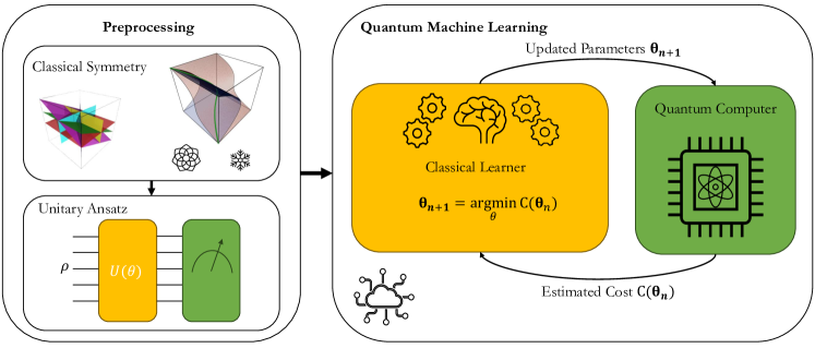
Figure 1: Symmetry Imposed Ansätze in QML. Control parameters of a quantum computer are trained via a classical learner in the cloud to minimize a cost function. Before the training can begin, a parameterized unitary $U(\theta)$, must be selected during the preprocessing. Classical symmetries inform the selection of an ansatz; that is, the classical invariance should be imposed on the ansatz. The ansatz determines what gates will be applied during a computation on the quantum computer and how these gates are parameterized.

In this manuscript, we delineate the mathematical foundations for a large class of ansatze: driver or mixers (at sufficient depth) that can explore (including irreducibly) a subspace constrained to a classical symmetry. Such drivers and mixers have been studied in the context of optimization problems since at least Ref. [15]. Determining an appropriate driver Hamiltonian [6, 7, 16] or circuit ansatz [13, 21, 27, 33, 43] is a central task for achieving maximum utility of quantum computers. Especially in the context of variatonal quantum algorithms (VQAs) [28, 22] and NISQ [19] quantum annealing [15, 14, 42] (QA), ansatz construction has become a major focal point for modern quantum algorithms. Despite many exciting avenues and important fundamental results on the value proposition of different ansatz constructions, ansatz selection largely remains an art within a very general mathematical framework. Given a specific hardware set and problem of interest, selecting the best ansatz based on some criteria is one of the most important challenges in quantum heuristics today.

Consider a general constrained optimization problem over binary variables $x=(x_{1},\ldots,x_{n})\in\mathbb{Z}_{2}^{n}$ with a set of constraints $\mathcal{C}=\{C_{1},\ldots,C_{m}\}$, where $C_{i}(x)=b_{i}$ is an equality polynomial constraint function for some $b_{i}$. Then we desire to minimize an objective polynomial function $f(x)$ while satisfying each constraint. The constraint optimization problem can then be written as:

$$\min\; f(x)$$

subject to $$C_{i}(x)=b_{i},\;\text{for}\;i\in[1,\ldots,m]$$ (1)

Inequality constraints can be dealt with in a number of ways through this formulation; such constraints can be turned into soft constraints through penalty terms, tracked with ancilla qubits, transformed into equality constraints with slack variables, enforced through other quantum effects like Zeno processes [39], or cast into high(er) order polynomial equality constraints (to name a few).

Ref. [41] considers equality constraints with slack variables for a single global inequality constraint. Ref. [10] considers quadratic unconstrained binary optimization formulations for many NP-Hard problems, with inequality conditions enforced by several penalty terms.

Quantum Alternating Operator Ansatz (QAOA) and Constrained Quantum Annealing (CQA) share a similar assumption for solving optimization problems. Each bit $x_{i}\in\{0,1\}$ of $x$ is mapped to $\left\lvert\,x_{i}\,\right\rangle\in\{\left\lvert\,0\,\right\rangle,\left\lvert\,1\,\right\rangle\}$, such that $\left\lvert\,x\,\right\rangle=\left\lvert\,x_{1}\,\right\rangle\cdots\left\lvert\,x_{n}\,\right\rangle\in\{\left\lvert\,0\,\right\rangle,\left\lvert\,1\,\right\rangle\}^{\otimes n}$. Then each constraint is mapped to a constraint embedded operator $\hat{C}$ that is an observable over the computational basis such that $C(x)=\left\langle\,x\,\right\rvert\hat{C}\left\lvert\,x\,\right\rangle$ for any $x$.

Under nonrelativistic closed dynamics governed by a Hamiltonian $H(t)$, if $\left\langle\,\psi(0)\,\right\rvert\hat{C}\left\lvert\,\psi(0)\,\right\rangle=b$ at time $t=0$ and $[\hat{C},H]=0$, then $\left\langle\,\psi(t)\,\right\rvert\hat{C}\left\lvert\,\psi(t)\,\right\rangle=b$ for all time $t$. Hence, $\hat{C}$ is an invariant observable over $\left\lvert\,\psi(t)\,\right\rangle$ and $H$ maintains the symmetry imposed by $C$. CQA attempts to (approximately) minimize the optimization function $f(x)$ within the constraint space. Let

$$\hat{F}=\sum_{x\in F}\left\lvert\,x\,\right\rangle\!\left\langle\,x\,\right\rvert,\;F=\{x\,|\,x\in\{0,1\}^{n},\;C_{i}(x)=b_{i}\;\forall C_{i}\in\mathcal{C}\}$$ (2)

represent the projection operator into the embedded feasible space for a collection of constraints $\mathcal{C}$. If the optimization function, $f(x)$, is a constant function, the problem is a constraint satisfaction problem. Notice that any operator written in the computational basis (e.g. within the space $\text{span}(\{\mathbbm{1},\sigma^{z}\}^{\otimes n})$) will commute with $\hat{C}$ since they are mutually diagonalizable in the computational basis.

Standard CQA then attempts to solve a constrained optimization problem by constructing a dynamic Hamiltonian $H(t)=A(t)\,H_{d}+B(t)\,H_{f}$, where $H_{d}$ is a driver Hamiltonian and $H_{f}$ is the embedded cost operator for $f(x)$. If $\left\lvert\,\psi(0)\,\right\rangle$ is in the feasibility space, $\left\langle\,\psi(0)\,\right\rvert\hat{F}\left\lvert\,\psi(0)\,\right\rangle=1$, and $[\hat{C}_{i},H_{d}]=0$ for all $i$, then $\left\langle\,\psi(t)\,\right\rvert\hat{F}\left\lvert\,\psi(t)\,\right\rangle=1$ for any time $t$. As such, $\left\lvert\,\psi(t)\,\right\rangle$ will evolve within the constraint space. If $H_{d}$ irreducibly commutes with $\mathcal{C}$, $\left\lvert\,\psi(0)\,\right\rangle$ is a (approximate) ground state of $H_{d}$, and there is a smooth evolution from $A(0)=A,B(0)=0$ to $A(T)=0,B(T)=B$, then the adiabatic theorem states that $\left\lvert\,\psi(T)\,\right\rangle$ is a (approximate) ground state of $H_{f}$ for sufficiently large total time $T$.

An analogous discussion can be found in QAOA. Standard QAOA of $p$-depth is described by the application of two unitaries for $p$ rounds. H-QAOA [22] refers to the closest relative to CQA, $U(\vec{\alpha},\vec{\beta})=U(\beta_{p},\alpha_{p})\cdots U(\beta_{1},\alpha_{1})$ where $U(\alpha_{j},\beta_{j})=U_{m}(\beta_{j})U_{c}(\alpha_{j})$ with $U_{c}(\alpha_{j})=e^{-i\,\alpha_{j}\,H_{f}}$ and $U_{m}(\beta_{j})=e^{-i\,\beta_{j}\,H_{d}}$ for $\vec{\alpha},\vec{\beta}\in[0,2\,\pi]^{p}$ (or more generally $\vec{\alpha},\vec{\beta}\in\mathbb{R}_{+}^{p}$ depending on energy scalings). If angles $\vec{\alpha},\vec{\beta}$ are selected small enough, this becomes a Trotterization of CQA [44]. QAOA more generally considers alternative formulations for what is often called the mixing operator $U_{m}$, in place of what $e^{-i\,\beta\,H_{d}}$ accomplishes in H-QAOA, since $e^{-i\,\beta\,H_{d}}$ can be difficult to implement and can require high depth circuits.

The phase-separation operator, which introduces phases in the computational basis based on the quality of a state written in that basis, typically utilizes the cost function $f(x)$: $U_{c}(\alpha)=e^{-i\,\alpha\,H_{f}}$. Hence the phase of a computational basis state $\left\lvert\,x\,\right\rangle$ during one round is dependent on its cost, $U_{c}(\alpha)\left\lvert\,x\,\right\rangle=e^{i\,\alpha\,f(x)}\left\lvert\,x\,\right\rangle$. $H_{f}$ is composed of terms written in the computational basis and therefore each term commutes with one another. Typically, as for NP-Hard optimization problems, $H_{f}$ is made of several local body terms, $H_{f}=\sum_{t}H_{t}$, where each $H_{t}$ is a Hermitian operator acting on a fixed number of qubits (not dependent on $n$) and so the phase-separation operator can be written as $U_{c}(\alpha)=e^{i\,\alpha\,\sum_{t}H_{t}}=\prod_{t}e^{-i\,\alpha\,H_{t}}$.

The mixing operator, as the name implies, nontrivially mixes states written in the computational basis with their neighbors based on the action of each mixer in the mixing operator. However, $H_{d}$ could be composed of many noncommuting (and typically acting on only a fixed number of qubits) terms: $H_{d}=-\sum_{g\in G}H_{g}$ for a set $G$ of indices or mappings. Then $e^{i\,H_{d}}$ may be impractical to implement or require high depth circuits due to this noncommutativity. However, the set of generators $G$ can be partitioned in to $\mathcal{G}=\{G_{1},\ldots,G_{k}\}$ such that for all $g_{ij},g_{ik}\in G_{i}$, $[H_{g_{ij}},H_{g_{ik}}]=0$ and the disjoint union $\coprod_{G_{i}\in\mathcal{G}}G_{i}=G$. Then the mixer is transpiled as $U_{m}(\beta)=\prod_{G_{i}\in\mathcal{G}}\prod_{g\in G_{i}}e^{-i\,\beta\,g}$, which can have a significantly lower circuit depth to implement than $e^{i\,H_{d}}$.

A central question in both approaches is then how to find a suitable collection of terms $H_{g}$ such that $[\hat{C_{i}},H_{g}]=0$ for all $g$ and all $i$. This is discussed as an algebraic question Section 3, developed into an algorithmic problem from a complexity theory perspective in Section 4 and then practical algorithms to solve this problem are provided in Section 6. An interesting application of these concepts is then showcased on 1-in-3 SAT, a constraint satisfaction problem with a sparse number of local constraints, in Sec. 7.

3 Algebraic Conditions for Imposing Constraints

	Basis	N	S	L	H	O
1	$\{\mathbbm{1},\sigma^{x},\sigma^{y},\sigma^{z}\}^{\otimes n}$	False	False	True	True	False
2	$\{\mathbbm{1},\sigma^{z},\sigma^{-},\sigma^{+}\}^{\otimes n}$	False	True	True	False	False
3	$\{\sigma^{0},\sigma^{1},\sigma^{-},\sigma^{+}\}^{\otimes n}$	True	True	False	False	False
4	$\{\mathbbm{1},\sigma^{0},\sigma^{1},\sigma^{-},\sigma^{+}\}^{\otimes n}$	True	True	True	False	True

Table 1: Properties of Different Qubit Basis. Classification of the properties of different basis for complex matrices over $\mathbbm{C}^{2^{n}}$ with the mapping (N) for necessarily zero ((S) for sufficient to show zero) if a basis term is used for commuting with an embedded constraint operator (Eq. 3). (L) is for admitting local operators, (H) is if the basis terms are all Hermitian, and (O) is if the basis is overcomplete (the number of matrices is larger than the dimension of the matrix space). (1) is the Pauli basis. (4) is the focus of this section, which we show satisfies conditions (N), (S), and (L) that are important for algorithmic primitives used for complexity results in Sec. 4 and application in Sec. 6. It is not (H) and it is (O). Hermiticity is enforced by requiring a term’s transpose with the coefficient set as its complex conjugate. Overcompleteness is resolved by always selecting the most local representation. (3) satisfies (N) and (S), but is not (L), (H), or (O), while (2) satisfies (S) and (L), but is not (N), (H), or (O). However, (2) is (N) for linear constraints and discussed in App. A for enforcing (2-local and higher) Ising spin-z Hamiltonians.

In this section we derive a necessary and sufficient condition for a Hamiltonian to commute with a polynomial embedded constraint operator. This condition, Thm. 3.1, is utilized in Sec. 4 to show that finding local Hamiltonians that commute with embedded constraints is a task in polynomial time and Sec. 6 discusses practical algorithms for utilizing Thm. 3.1 to find a basis for nontrivial operators over the embedded feasible space. Tab. 1 shows the properties of several basis for writing complex matrices in $\mathbbm{C}^{2^{n}\times 2^{n}}$, with the unique property of the basis discussed in this section being that it admits a description of local operators and that commutation with an embedded constraint operator for a Hamiltonian written over the basis is zero if and only if commutation with each individual basis is zero. This locality condition and the commutation being necessary and sufficient is unique to this basis, see Tab. 1 for descriptions of other candidate basis.

Let $\sigma^{x},\sigma^{z},\sigma^{y}$ represent the standard Pauli matrices. Then let:

$$\sigma^{0} =\left\lvert\,0\,\right\rangle\!\left\langle\,0\,\right\rvert=\left(\mathbbm{1}+\sigma^{z}\right)/2,$$

$$\sigma^{1} =\left\lvert\,1\,\right\rangle\!\left\langle\,1\,\right\rvert=\left(\mathbbm{1}-\sigma^{z}\right)/2,$$

$$\sigma^{-} =\left\lvert\,0\,\right\rangle\!\left\langle\,1\,\right\rvert=\left(\sigma^{x}+i\,\sigma^{y}\right)/2,$$

$$\sigma^{+} =\left\lvert\,1\,\right\rangle\!\left\langle\,0\,\right\rvert=\left(\sigma^{x}-i\,\sigma^{y}\right)/2.$$ (3)

Left and right multiplication identities for these matrices are found in Appendix B and are useful for derivations within this section. A useful definition used throughout this manuscript is for a single term $T$ over the overcomplete operator basis $\{\mathbbm{1},\sigma^{0},\sigma^{1},\sigma^{-},\sigma^{+}\}^{\bigotimes n}$ (for $\mathbbm{C}^{2\times 2}$):

$$T(\vec{x},\vec{y},\vec{v},\vec{w})=\prod_{j=1}^{n}\bigg{(}\sigma_{j}^{0}\bigg{)}^{x_{j}}\bigg{(}\sigma_{j}^{1}\bigg{)}^{y_{j}}\bigg{(}\sigma_{j}^{+}\bigg{)}^{v_{j}}\bigg{(}\sigma_{j}^{-}\bigg{)}^{w_{j}},$$ (4)

where $\vec{x},\vec{y},\vec{v},\vec{w}$ are assumed to be orthogonal binary vectors. By the facts ${\sigma^{-}}^{\dagger}=\sigma^{+}$, ${\sigma^{0}}^{\dagger}=\sigma^{0}$, and ${\sigma^{1}}^{\dagger}=\sigma^{1}$ as well as the distribution of the adjoint operator over tensor products, we have:

$$T(\vec{x},\vec{y},\vec{v},\vec{w})=T^{\dagger}(\vec{x},\vec{y},\vec{w},\vec{v}).$$ (5)

For any polynomial constraint, $C(x)$, we can find the corresponding eigenspace decomposition for different equality values $b$ representing the associated feasibility space of the constraint problem with $C(x)$ fixed to the value $b$ as:

$$F_{b}=\{x\,|\,C(x)=b,\,x\in\{0,1\}^{n}\}.$$ (6)

Then the associated projection operator of the embedded eigenspace (embedded feasibility subspace) assuming $\hat{C}$ has the constraint value as the eigenvalue for each eigenspace:

$$\hat{F}_{b} =\sum_{x\in F_{b}}\left\lvert\,x\,\right\rangle\!\left\langle\,x\,\right\rvert.$$ (7)

Any polynomial constraint over binary variables $x\in\{0,1\}^{n}$ can be written in the form:

$$C(x)=\sum_{(\vec{a_{J}},\vec{b_{J}})\in\mathcal{J}}\beta_{J}\,\prod_{k=1}^{n}(1-x_{i})^{a_{Jk}}\,x_{i}^{b_{Jk}},$$ (8)

where each $(\vec{a_{J}},\vec{b_{J}})\in\mathcal{J}$ is orthogonal binary vectors and each $\beta_{J}$ is assumed nonzero. Under the standard bit to qubit mapping $\left\lvert\,x\,\right\rangle=\left\lvert\,x_{1}\,\right\rangle\ldots\left\lvert\,x_{n}\,\right\rangle\in\{\left\lvert\,0\,\right\rangle,\left\lvert\,1\,\right\rangle\}^{n}$, we consider the natural embedding to be $\hat{C}$ such that $\left\langle\,x\,\right\rvert\hat{C}\left\lvert\,x\,\right\rangle=C(x)=b$. The constraint is embedded as:

$$\hat{C} =\sum_{(\vec{a_{J}},\vec{b_{J}})\in\mathcal{J}}\beta_{J}\,\prod_{k=1}^{n}\left(\sigma_{k}^{0}\right)^{a_{Jk}}\left(\sigma_{k}^{1}\right)^{b_{Jk}}$$

$$=\sum_{(\vec{a_{J}},\vec{b_{J}})\in\mathcal{J}}\beta_{J}\,T(\vec{a_{J}},\vec{b_{J}},\mathbf{0},\mathbf{0}),$$ (9)

where every $(\vec{a_{J}},\vec{b_{J}})\in\mathcal{J}$ are orthogonal binary vectors and each $\beta_{J}$ is assumed nonzero. Then:

$$\left\langle\,x\,\right\rvert\hat{C}\left\lvert\,x\,\right\rangle =\sum_{(\vec{a_{J}},\vec{b_{J}})\in\mathcal{J}}\beta_{J}\,\prod_{k=1}^{n}\left\langle\,x\,\right\rvert\left(\sigma_{k}^{0}\right)^{a_{Jk}}\left(\sigma_{k}^{1}\right)^{b_{Jk}}\left\lvert\,x\,\right\rangle$$

$$=\sum_{(\vec{a_{J}},\vec{b_{J}})\in\mathcal{J}}\beta_{J}\,\prod_{k=1}^{n}\left\langle\,x_{i}\,\right\rvert\left(\sigma^{0}\right)^{a_{Jk}}\left(\sigma^{1}\right)^{b_{Jk}}\left\lvert\,x_{i}\,\right\rangle$$

$$=\sum_{(\vec{a_{J}},\vec{b_{J}})\in\mathcal{J}}\beta_{J}\,\prod_{k=1}^{n}\Theta(1-x_{i})^{a_{Jk}}\Theta(x_{i})^{b_{Jk}}$$

$$=\sum_{(\vec{a_{J}},\vec{b_{J}})\in\mathcal{J}}\beta_{J}\,\prod_{k=1}^{n}(1-x_{i})^{a_{Jk}}x_{i}^{b_{Jk}},$$ (10)

where $\Theta(x)$ is the Heaviside step function such that $\Theta(x)=1$ if $x>0$ and $\Theta(x)=0$ if $x\leq 0$. Eq. 3 is the natural embedding since the correspondents between Eq. 6 and Eq. 7 is that $\left\langle\,x\,\right\rvert\hat{C}\left\lvert\,x\,\right\rangle=b$ for $\left\lvert\,x\,\right\rangle$ in $F_{b}$ precisely for this operator. While this is the natural embedding, other embeddings have been studied more in part due to the prevalence of Ising spin formalisms [10, 14, 15].

A prototypical, widely studied case is that of a single global constraint $C(x)=\sum_{i}^{n}x_{i}=b$ for some $b$. This constraint is utilized in graph partitioning and portfolio optimization among others. Then the natural embedding constraint operator is $\hat{C}=\sum_{i}^{n}\sigma_{i}^{1}=b$. Other embeddings would be $\hat{C}=\sum_{i}^{n}\sigma_{i}^{0}=n-b$ and $\hat{C}=\sum_{i}^{n}\sigma_{i}^{0}-\sigma_{i}^{1}=\sum_{i}^{n}\sigma_{i}^{z}=n-2\,b$. Such embeddings are equivalent in their eigenspaces, but not their corresponding eigenvalues, so finding commutative terms for one is associated with the same (eigenspace) invariance as the other embedding, but the expected value of the associated observables differ.

An example of this type of mapping with linear constraints is discussed in Sec. 7 and appears in the early Ref. [2] (among many other papers) in the context of quantum annealing. We assume that $\hat{C}$ is always simplified to use the minimum number of non-zero entries (e.g. simplify cases where an identity can replace two like terms that differ only by having $\sigma^{0}$ versus $\sigma^{1}$ on some qubit shared on an entry).

Linear operators that commute with $\hat{F}_{b}$ are operators over the matrix span:

$$\mathcal{F}_{b}=\text{span}\left(\{\left\lvert\,x\,\right\rangle\!\left\langle\,y\,\right\rvert\,|\,x,y\in F_{b}\}\right),$$ (11)

which we call the commutation space over the feasible subspace $F_{b}$ and is a subspace of linear operators $\mathbbm{C}^{2^{n}\times 2^{n}}$. Given a specific feasible state $x$ such that $\left\lvert\,x\,\right\rangle\in\hat{F}_{b}$, we know that for $H$ to commute with $\hat{C}$, $H\left\lvert\,x\,\right\rangle\in\hat{F}_{b}$, otherwise the degenerate eigenspace symmetry of $F_{b}$ is broken. As such, $\hat{F}_{b}H\hat{F}_{b}\in\mathcal{F}_{b}$ if and only if $\hat{F}_{b}H\hat{F}_{b}$ commutes with the constraint $\hat{C}$. In particular, $H$ commutes with $\hat{C}$ if and only if the condition holds for every $b$ and $H$ is then said to be in the commutation space of $\hat{C}$. This generalizes to multiple constraints; if and only if the condition holds for every $\hat{C}$ does $H$ commute with the embedded constraints and is in the associated commutation space.

This includes all diagonal matrices, i.e. $[H,\hat{C}]=0$ if $H$ has no nonzero offdiagonal element over the computational basis and so we say $H$ commutes nontrivially with $\hat{C}$ if $H$ has at least one offdiagonal term.

Any Hermitian matrix $H$ over $\mathbbm{C}^{2^{n}}$ can be written over the overcomplete basis $\{\mathbbm{1},\sigma^{0},\sigma^{1},\sigma^{+},\sigma^{-}\}^{\bigotimes n}$ as:

$$H =\sum_{(\vec{x_{j}},\vec{y_{j}},\vec{v_{j}},\vec{w_{j}})\in\Delta(\mathscr{X},\;\mathscr{Y},\;\mathscr{V},\;\mathscr{W})}\alpha_{j}\;T(\vec{x_{j}},\vec{y_{j}},\vec{v_{j}},\vec{w_{j}})+\alpha_{j}^{\dagger}\;T(\vec{x_{j}},\vec{y_{j}},\vec{w_{j}},\vec{v_{j}}),$$ (12)

following a similar convention as Ref. [32], where $\Delta(\mathscr{X},\mathscr{Y},\mathscr{V},\mathscr{W})$ represents the set of index-wise confederated tuples. On a matrix $H$, $H^{\dagger}$ is the complex conjugate transpose of $H$ and so in Eq. 12 $,\alpha_{j}^{\dagger}$ is the complex conjugate of a scalar $\alpha\in\mathbbm{C}$. By utilizing Eq. 5, notice that $H$ is indeed Hermitian:

$$H^{\dagger} =\sum_{(\vec{x_{j}},\vec{y_{j}},\vec{v_{j}},\vec{w_{j}})\in\Delta(\mathscr{X},\;\mathscr{Y},\;\mathscr{V},\;\mathscr{W})}\alpha_{j}^{\dagger}\;T^{\dagger}(\vec{x_{j}},\vec{y_{j}},\vec{v_{j}},\vec{w_{j}})+\alpha_{j}\;T^{\dagger}(\vec{x_{j}},\vec{y_{j}},\vec{w_{j}},\vec{v_{j}})$$

$$=\sum_{(\vec{x_{j}},\vec{y_{j}},\vec{v_{j}},\vec{w_{j}})\in\Delta(\mathscr{X},\;\mathscr{Y},\;\mathscr{V},\;\mathscr{W})}\alpha_{j}^{\dagger}\;T(\vec{x_{j}},\vec{y_{j}},\vec{w_{j}},\vec{v_{j}})+\alpha_{j}\;T(\vec{x_{j}},\vec{y_{j}},\vec{v_{j}},\vec{w_{j}})$$

$$=H.$$ (13)

As an example of this formalism, consider the Hermitian matrix:

$$\sigma_{1}^{0}\sigma_{2}^{1}\left(\sigma_{3}^{+}\sigma_{4}^{-}+\sigma_{3}^{+}\sigma_{4}^{-}\right) =T((1,0,0,0),(0,1,0,0),(0,0,1,0),(0,0,0,1))$$

$$\phantom{=}+T((1,0,0,0),(0,1,0,0),(0,0,0,1),(0,0,1,0)),$$ (14)

with ordered sets $\mathscr{X}=\{(1,0,0,0)\}$, $\mathscr{Y}=\{(0,1,0,0)\}$, $\mathscr{V}=\{(0,0,1,0)\}$, $\mathscr{W}=\{(0,0,0,1)\}$.

Although somewhat tedious, this formalism representing the choice function on each qubit for each term over the chosen (overcomplete) basis is of practical usefulness for deriving algebraic forms to reason about imposing symmetries. In the form we will consider throughout the manuscript, redundant forms are removed or reduced before consideration (a similar discussion appears in Ref. [32]) by removing any terms with $\alpha_{j}=\alpha_{j}^{\dagger}=0$ and reducing $\mathscr{X},\mathscr{Y}$ as much as possible if the identity term can be utilized.

Using this basis, we state our first algebriac result as a theorem for recognizing if a Hermitian matrix commutes with a general constraint.

Theorem 3.1.

A general Hermitian matrix $H(\mathscr{X},\mathscr{Y},\mathscr{V},\mathscr{W})$ commutes with a general constraint $\hat{C}(\mathcal{J})$ iff, for all $\vec{x},\vec{y},\vec{v},\vec{w}\in\Delta(\mathscr{X},\mathscr{Y},\mathscr{V},\mathscr{W})$:

$$\sum_{(\vec{a_{J}},\vec{b_{J}})\in\mathcal{J}}\beta_{J}\bigg{(}\left(1-\Theta((\vec{y_{j}}+\vec{w_{j}})\cdot\vec{a_{J}}+(\vec{x_{j}}+\vec{v_{j}})\cdot\vec{b_{J}})\right)$$

$$\phantom{\sum}-\left(1-\Theta((\vec{y_{j}}+\vec{v_{j}})\cdot\vec{a_{J}}+(\vec{x_{j}}+\vec{w_{j}})\cdot\vec{b_{J}})\right)\bigg{)}T(\vec{x_{j}}+(\mathbf{1}-\vec{v_{j}}-\vec{x_{j}})\circ\vec{a_{J}},\vec{y_{j}}+(\mathbf{1}-\vec{w_{j}}-\vec{y_{j}})\circ\vec{b_{j}},\vec{v_{j}},\vec{w_{j}})$$

$$+\sum_{(\vec{a_{J}},\vec{b_{J}})\in\mathcal{J}}\beta_{J}\bigg{(}\left(1-\Theta((\vec{y_{j}}+\vec{v_{j}})\cdot\vec{a_{J}}+(\vec{x_{j}}+\vec{w_{j}})\cdot\vec{b_{J}})\right)$$

$$\phantom{=}-\left(1-\Theta((\vec{y_{j}}+\vec{v_{j}})\cdot\vec{a_{J}}+(\vec{x_{j}}+\vec{w_{j}})\cdot\vec{b_{J}})\right)\bigg{)}T(\vec{x_{j}}+(\mathbf{1}-\vec{w_{j}}-\vec{x_{j}})\circ\vec{a_{J}},\vec{y_{j}}+(\mathbf{1}-\vec{v_{j}}-\vec{y_{j}})\circ\vec{b_{j}},\vec{w_{j}},\vec{v_{j}})=0,$$ (15)

where $\Theta$ is the Heaviside step function, $\mathbf{1}$ is the all ones vector $(1,1,\ldots,1)$ and $\circ$ is the element-wise (Hadamard) product between vectors: $\vec{a}\circ\vec{b}=(a_{1}b_{1},\ldots,a_{n}b_{n})$.

Proof.

Thm. 3.1 is built on a commutation relationship of general interest:

$$\left[H,\hat{C}\right] =\left[\sum_{(\vec{x_{j}},\vec{y_{j}},\vec{v_{j}},\vec{w_{j}})\in\Delta(\mathscr{X},\;\mathscr{Y},\;\mathscr{V},\;\mathscr{W})}\alpha_{j}\;T(\vec{x_{j}},\vec{y_{j}},\vec{v_{j}},\vec{w_{j}})+\alpha_{j}^{\dagger}\;T(\vec{x_{j}},\vec{y_{j}},\vec{w_{j}},\vec{v_{j}}),\sum_{(a_{J},b_{J})\in\mathcal{J}}\beta_{J}\,T(\vec{a_{J}},\vec{b_{J}},0,0)\right]$$

$$=\sum\sum\alpha_{j}\,\beta_{J}\,\bigg{(}\left(1-\Theta((\vec{y_{j}}+\vec{w_{j}})\cdot\vec{a_{J}}+(\vec{x_{j}}+\vec{v_{j}})\cdot\vec{b_{J}})\right)$$

$$\phantom{=\sum}-\left(1-\Theta((\vec{y_{j}}+\vec{v_{j}})\cdot\vec{a_{J}}+(\vec{x_{j}}+\vec{w_{j}})\cdot\vec{b_{J}})\right)\bigg{)}T(\vec{x_{j}}+(\mathbf{1}-\vec{v_{j}}-\vec{x_{j}})\circ\vec{a_{J}},\vec{y_{j}}+(\mathbf{1}-\vec{w_{j}}-\vec{y_{j}})\circ\vec{b_{j}},\vec{v_{j}},\vec{w_{j}})$$

$$\phantom{=}+\sum\sum\alpha_{j}^{\dagger}\,\beta_{J}\,\bigg{(}\left(1-\Theta((\vec{y_{j}}+\vec{v_{j}})\cdot\vec{a_{J}}+(\vec{x_{j}}+\vec{w_{j}})\cdot\vec{b_{J}})\right)$$

$$\phantom{=\sum}-\left(1-\Theta((\vec{y_{j}}+\vec{w_{j}})\cdot\vec{a_{J}}+(\vec{x_{j}}+\vec{v_{j}})\cdot\vec{b_{J}})\right)\bigg{)}T(\vec{x_{j}}+(\mathbf{1}-\vec{w_{j}}-\vec{x_{j}})\circ\vec{a_{J}},\vec{y_{j}}+(\mathbf{1}-\vec{v_{j}}-\vec{y_{j}})\circ\vec{b_{j}},\vec{w_{j}},\vec{v_{j}}).$$ (16)

By recognizing the orthogonality of the basis (if $H$ has nonorthogonal terms, they can be reduced to be orthogonal) and setting Eq. 3 $=0$, the sufficient condition follows immediately. We show necessity first and then derive Eq. 3.

Right (left) commutation by a given matrix, $\hat{C}$, is a linear transformation over matrices, since $[M_{1}+M_{2},\hat{C}]=[M_{1},\hat{C}]+[M_{2},\hat{C}]$ for any matrices $M_{1},M_{2}\in\mathbbm{C}^{2^{n}\times 2^{n}}$. For necessity of the condition, we show that the formalism can express the span of the kernel. Using the feasibility decomposition $\hat{C}=\sum b_{i}\hat{F}_{b_{i}}$ from Eq. 7, the kernel of right commutation with $\hat{C}$ is spanned by operators that map feasible states to other feasible states. Let $x,y\in F_{b}$, such that $\left\langle\,x\,\right\rvert\hat{F}_{b}\left\lvert\,x\,\right\rangle=\left\langle\,y\,\right\rvert\hat{F}_{b}\left\lvert\,y\,\right\rangle=1$ for a specific $b$, then:

$$\left\lvert\,x\,\right\rangle\!\left\langle\,y\,\right\rvert =\bigotimes_{i=1}^{n}\big{(}\left\lvert\,x_{i}\,\right\rangle\!\left\langle\,y_{i}\,\right\rvert\big{)}$$

$$=\bigotimes_{i=1}^{n}\left(\sigma_{i}^{0}\right)^{(1-x_{i})(1-y_{i})}\left(\sigma_{i}^{1}\right)^{x_{i}y_{i}}\left(\sigma_{i}^{+}\right)^{x_{i}(1-y_{i})}\left(\sigma_{i}^{-}\right)^{(1-x_{i})y_{i}}.$$ (17)

Then, $\left\lvert\,x\,\right\rangle\!\left\langle\,y\,\right\rvert$ is a term in our formalism and the entire kernel (i.e. commutation space) can be spanned by such terms. In particular, there are $|F_{b}|^{2}$ such terms for a specific $b$, by restricting to nontrivial commutators $|F_{b}|^{2}-|F_{b}|$. This shows necessity.

By using the overcomplete operator basis, we allow for lower locality terms by recognizing commonalities between different mappings (including between different constraint spaces). For example, suppose we consider the constraint $C\equiv x_{1}=1$ over 2 bits $\{0,1\}^{2}$ so that $\hat{C}=\sigma_{1}^{1}$ over $2$ qubits, such that $F_{0}=\{(0,0),(0,1)\}$ and $F_{1}=\{(1,0),(1,1)\}$ and therefore $\hat{F}_{0}=\left\lvert\,00\,\right\rangle\!\left\langle\,00\,\right\rvert+\left\lvert\,01\,\right\rangle\!\left\langle\,01\,\right\rvert$ and $\hat{F}_{1}=\left\lvert\,10\,\right\rangle\!\left\langle\,10\,\right\rvert+\left\lvert\,11\,\right\rangle\!\left\langle\,11\,\right\rvert$. Then $\{\sigma_{1}^{0}\sigma_{2}^{+},\sigma_{1}^{0}\sigma_{2}^{-}\}$ are a basis for the nontrivial commutators restricted to $F_{0}$ while $\{\sigma_{1}^{1}\sigma_{2}^{+},\sigma_{1}^{1}\sigma_{2}^{-}\}$ are a basis for the nontrivial commutators restricted to $F_{1}$. However, with the overcomplete basis that includes $\mathbbm{1}$, we can utilize the more local forms $\{\sigma_{2}^{+},\sigma_{2}^{-}\}$. As such, both $\alpha\,\sigma_{2}^{+}+\alpha^{\dagger}\,\sigma_{2}^{-}$ and $\alpha\,\sigma_{1}^{1}\sigma_{2}^{+}+\alpha^{\dagger}\,\sigma_{1}^{1}\sigma_{2}^{-}$ end up having the same relevant action for the feasibility subspace of interest (for any fixed $\alpha\in\mathbbm{C}$).

For sufficency, we show how to derive Eq. 3. Beginning with the definitions Eq. 3 and Eq. 12:

$$\left[H,\hat{C}\right] =\sum_{(\vec{x_{j}},\vec{y_{j}},\vec{v_{j}},\vec{w_{j}})\in\Delta(\mathscr{X},\;\mathscr{Y},\;\mathscr{V},\;\mathscr{W})}\left[\alpha_{j}\,\prod_{i=1}^{n}\left(\sigma_{i}^{0}\right)^{x_{ji}}\left(\sigma_{i}^{1}\right)^{y_{ji}}\left(\sigma_{i}^{+}\right)^{v_{ji}}\left(\sigma_{i}^{-}\right)^{w_{ji}},\sum_{(a_{J},b_{J})\in\mathcal{J}}\beta_{J}\,\prod_{k=1}^{n}\left(\sigma_{k}^{0}\right)^{a_{Jk}}\left(\sigma_{k}^{1}\right)^{b_{Jk}}\right]$$

$$\phantom{=}+\sum_{(\vec{x_{j}},\vec{y_{j}},\vec{v_{j}},\vec{w_{j}})\in\Delta(\mathscr{X},\;\mathscr{Y},\;\mathscr{V},\;\mathscr{W})}\left[\alpha_{j}^{\dagger}\,\prod_{i=1}^{n}\left(\sigma_{i}^{0}\right)^{x_{ji}}\left(\sigma_{i}^{1}\right)^{y_{ji}}\left(\sigma_{i}^{+}\right)^{w_{ji}}\left(\sigma_{i}^{-}\right)^{v_{ji}},\sum_{(a_{J},b_{J})\in\mathcal{J}}\beta_{J}\,\prod_{k=1}^{n}\left(\sigma_{k}^{0}\right)^{a_{Jk}}\left(\sigma_{k}^{1}\right)^{b_{Jk}}\right]$$

$$=\sum_{(\vec{x_{j}},\vec{y_{j}},\vec{v_{j}},\vec{w_{j}})\in\Delta(\mathscr{X},\;\mathscr{Y},\;\mathscr{V},\;\mathscr{W})}\alpha_{j}\,\sum_{(a_{J},b_{J})\in\mathcal{J}}\beta_{J}\,L_{jK}(\vec{a_{J}},\vec{b_{J}},\vec{x_{j}},\vec{y_{j}},\vec{v_{j}},\vec{w_{j}})$$

$$\phantom{=}+\sum_{(\vec{x_{j}},\vec{y_{j}},\vec{v_{j}},\vec{w_{j}})\in\Delta(\mathscr{X},\;\mathscr{Y},\;\mathscr{V},\;\mathscr{W})}\alpha_{j}^{\dagger}\,\sum_{(a_{J},b_{J})\in\mathcal{J}}\beta_{J}\,R_{jK}(\vec{a_{J}},\vec{b_{J}},\vec{x_{j}},\vec{y_{j}},\vec{v_{j}},\vec{w_{j}})$$ (18)

where:

$$L_{jK}(\vec{a},\vec{b},\vec{x},\vec{y},\vec{v},\vec{w}) =\prod_{k=1}^{n}\left(\sigma_{k}^{0}\right)^{x_{jk}}\left(\sigma_{k}^{1}\right)^{y_{jk}}\left(\sigma_{k}^{+}\right)^{v_{jk}}\left(\sigma_{k}^{-}\right)^{w_{jk}}\left(\sigma_{k}^{0}\right)^{a_{jk}}\left(\sigma_{k}^{1}\right)^{b_{jk}}$$

$$\phantom{=}-\prod_{k=1}^{n}\left(\sigma_{k}^{0}\right)^{a_{jk}}\left(\sigma_{k}^{1}\right)^{b_{jk}}\left(\sigma_{k}^{0}\right)^{x_{jk}}\left(\sigma_{k}^{1}\right)^{y_{jk}}\left(\sigma_{k}^{+}\right)^{v_{jk}}\left(\sigma_{k}^{-}\right)^{w_{jk}}$$

$$=\left(1-\Theta((\vec{y}+\vec{v})\cdot\vec{a}+(\vec{x}+\vec{w})\cdot\vec{b})\right)T(\vec{x}+(\mathbf{1}-\vec{w}-\vec{x})\circ\vec{a},\vec{y}+(\mathbf{1}-\vec{v}-\vec{y})\circ\vec{b},\vec{v},\vec{w})$$

$$\phantom{=}-\left(1-\Theta((\vec{y}+\vec{w})\cdot\vec{a}+(\vec{x}+\vec{v})\cdot\vec{b})\right)T(\vec{x}+(\mathbf{1}-\vec{v}-\vec{x})\circ\vec{a},\vec{y}+(\mathbf{1}-\vec{w}-\vec{y})\circ\vec{b},\vec{v},\vec{w})$$ (19)

and:

$$R_{jK}(\vec{a},\vec{b},\vec{x},\vec{y},\vec{v},\vec{w}) =\prod_{k=1}^{n}\left(\sigma_{k}^{0}\right)^{x_{jk}}\left(\sigma_{k}^{1}\right)^{y_{jk}}\left(\sigma_{k}^{+}\right)^{w_{jk}}\left(\sigma_{k}^{-}\right)^{v_{jk}}\left(\sigma_{k}^{0}\right)^{a_{jk}}\left(\sigma_{k}^{1}\right)^{b_{jk}}$$

$$\phantom{=}-\prod_{k=1}^{n}\left(\sigma_{k}^{0}\right)^{a_{jk}}\left(\sigma_{k}^{1}\right)^{b_{jk}}\left(\sigma_{k}^{0}\right)^{x_{jk}}\left(\sigma_{k}^{1}\right)^{y_{jk}}\left(\sigma_{k}^{+}\right)^{w_{jk}}\left(\sigma_{k}^{-}\right)^{v_{jk}}$$

$$=\left(1-\Theta((\vec{y}+\vec{w})\cdot\vec{a}+(\vec{x}+\vec{v})\cdot\vec{b})\right)T(\vec{x}+(\mathbf{1}-\vec{v}-\vec{x})\circ\vec{a},\vec{y}+(\mathbf{1}-\vec{w}-\vec{y})\circ\vec{b},\vec{w},\vec{v})$$

$$\phantom{=}-\left(1-\Theta((\vec{y}+\vec{v})\cdot\vec{a}+(\vec{x}+\vec{w})\cdot\vec{b})\right)T(\vec{x}+(\mathbf{1}-\vec{w}-\vec{x})\circ\vec{a},\vec{y}+(\mathbf{1}-\vec{v}-\vec{y})\circ\vec{b},\vec{w},\vec{v}),$$ (20)

with the $\Theta(x)$ as the Heaviside step function.

∎

It immediately follows that if this is true for a collection of constraints, that $H$ will commute with all of them. For several constraints of interest that are higher order than linear, a simple strategy is to match part of $\vec{y}$ and part of $\vec{x}$ to overlap with the given $\vec{a_{J}}$ and $\vec{b_{J}}$. For example, for the maximum independent set (MIS) problem, the popular ansatz given in Ref. [17] has this form.

The maximum independent set problem can be defined as a maximization problem with linear inequality constraints associated with a graph $G=(V,E)$ over $X=\{x_{1},\ldots,x_{n}\}$ and $x_{i}\in\{0,1\}$ with $x_{i}$ associated with vertex $v_{i}\in V$ and $|V|=n$:

maximize $$\;\sum_{i}x_{i}$$

subject to $$\;x_{i}+x_{j}\leq 1\;\text{for}\;(v_{i},v_{j})\in E$$ (21)

Alternatively, it can be cast as a polynomial equality constraint problem and a minimization problem:

minimize $$\;\sum_{i}^{n}(1-x_{i})$$

subject to $$\;\sum_{(v_{i},v_{j})\in E}x_{i}x_{j}=0$$ (22)

Then the embedded constraint operator can be written:

$$\hat{C}_{\text{mis}}=\sum_{(v_{i},v_{j})\in E}\sigma_{i}^{1}\sigma_{j}^{1}=0,$$ (23)

while the cost Hamiltonian can be:

$$H_{f,\text{mis}}=\sum_{i=1}^{n}\sigma_{i}^{0}.$$ (24)

Define $E(v_{i})=\{(v_{i},v_{j})\,|(v_{i},v_{j})\in E\}$ as the neighborhood edges of $v_{i}$. Then a term

$$T_{i,\text{mis}} =\sigma_{i}^{+}\prod_{(v_{i},v_{j})\in E(v_{i})}\sigma_{j}^{0}+\sigma_{i}^{-}\prod_{(v_{i},v_{j})}\sigma_{j}^{0}$$

$$=\sigma_{i}^{x}\prod_{(v_{i},v_{j})\in E}\sigma_{j}^{0},$$ (25)

commutes with the embedded equality constraint operators:

$$[T_{i,\text{mis}},\hat{C}_{\text{mis}}] =\sum_{(v_{k},v_{l})\in E}[T_{i,\text{mis}},\sigma_{k}^{1}\sigma_{l}^{1}]$$

$$=\sum_{(v_{k},v_{l})\in E}[\sigma_{i}^{+}\prod_{(v_{i},v_{j})\in E(v_{i})}\sigma_{j}^{0},\sigma_{k}^{1}\sigma_{l}^{1}]+[\sigma_{i}^{-}\prod_{(v_{i},v_{j})\in E(v_{i})}\sigma_{j}^{0},\sigma_{k}^{1}\sigma_{l}^{1}]$$

$$=\sum_{(v_{k},v_{l})\in E(v_{i})}[\sigma_{i}^{+}\prod_{(v_{i},v_{j})\in E(v_{i})}\sigma_{j}^{0},\sigma_{k}^{1}\sigma_{l}^{1}]+[\sigma_{i}^{-}\prod_{(v_{i},v_{j})\in E(v_{i})}\sigma_{j}^{0},\sigma_{k}^{1}\sigma_{l}^{1}]$$

$$=0.$$ (26)

Placing $\sigma_{j}^{0}$ for each neighbor $v_{j}$ of a node $v_{i}$ for the term $T_{i,\text{mis}}$ means that $[T_{i,\text{mis}},\sigma_{i}^{1}\sigma_{j}^{1}]=0$ because $\sigma_{j}^{0}\sigma_{j}^{1}=\sigma_{j}^{1}\sigma_{j}^{0}=0$. In fact, $\sum_{i=1}^{n}T_{i,\text{mis}}$ is a standard driver for exploiting this symmetry of MIS. Moreover, this driver and its associated mixer provide irreducible commutation (see Sec. 4). This example illustrates a simple means to satisfying higher order constraints: placing a single $\sigma^{0}$ ($\sigma^{1}$) term on a qubit where there is a term $\sigma^{1}$ ($\sigma^{0}$) in the constraint (provided at least one $\sigma^{+}$ or $\sigma^{-}$ has been placed to ensure off-diagonality). This motivates the formulation of a backtracking approach like Alg. 2 in Sec. 6.

Cast as a minimization problem, the cost Hamiltonian $H_{f,\text{min}}$ leads to the phase-separation operator $e^{-i\,\left(\sum_{i}\sigma^{0}\right)}=\prod_{i=1}^{n}e^{-i\,\sigma^{0}}$. As an initial state inside the constraint space, we can use the embedding of the empty independent set $\left\lvert\,\psi(0)\,\right\rangle=\left\lvert\,0\,\right\rangle\ldots\left\lvert\,0\,\right\rangle$ or an embedding of any valid independent set.

Note that the identity $[AB,C]=A[B,C]+[A,C]B$ implies that commutation is preserved under multiplication and the identity $[A+B,C]=[A,C]+[B,C]$ implies commutation is preserved under addition. Then finding a collection of terms $\mathcal{T}$, each commutative with the collection of constraints of interest, can be recognized as a commutator matrix ring (developed in Sec. 5). In particular, we develop algorithms to find such a set $\mathcal{T}$ that satisfies Thm. 3.1 for ansatz generation in Sec. 6.

In comparison to the expression derived in Appendix A, the inclusion of $\sigma^{0}$ and $\sigma^{1}$ leads to a more inclusive way to find terms that commute to constraints, while the expressions of Appendix A give a straight forward sufficient condition that generalizes the expression found in Ref. [32] and are more useful in situations where the basis $\{\mathbbm{1},\sigma^{z}\}^{\bigotimes n}$ is used, for example to express quantum Hamiltonians in the study of quantum materials or chemistry.

For completeness, we show how to recognize the main algebraic result in Ref. [32] within this formalism. Consider a linear constraint $C(x)=\sum_{j=1}^{n}c_{j}\,x_{j}$ that was embedded as $\hat{C^{\prime}}=\sum_{j=1}^{n}c_{j}\,\sigma_{j}^{z}=\sum_{j=1}^{n}c_{j}\,(2\sigma_{j}^{0}-\mathbbm{1})=\left(2\,\sum_{j=1}^{n}\sigma_{j}^{0}\right)-\left(\sum_{j=1}^{n}c_{j}\right)\mathbbm{1}$. Since the identity operator is in the kernel of any commutation, we would use the embedded operator $\hat{C}=\sum_{j=1}^{n}c_{j}\,\sigma_{j}^{0}$, and commutation with $\hat{C}$ implies commutation with $\hat{C^{\prime}}$ and vice versa. Same follows for embeddings utilizing $\sigma^{1}$ rather than $\sigma^{0}$ (as either choice is valid) as $\hat{C}^{\prime\prime}=\sum_{j=1}^{n}c_{j}\,\sigma_{j}^{1}=\sum_{j=1}^{n}c_{j}\,\left(\mathbbm{1}-\sigma_{j}^{0}\right)=\left(\sum_{j=1}^{n}c_{j}\right)\mathbbm{1}-\left(\sum_{j=1}^{n}c_{j}\,\sigma_{j}^{0}\right)$. Then Eq. 15 can be simplified as:

$$\sum_{j=1}^{n}c_{j}\left(\Theta(v_{j})-\Theta(w_{j})\right)=\vec{c}\cdot\left(\vec{v}-\vec{w}\right)=0,$$ (27)

since placing $x_{j}\neq 0$ or $y_{j}\neq 0$ is irrelevant for the commutation for any location and recognizing $\mathcal{J}=\{(\mathbf{e}_{1},\mathbf{0}),\ldots,(\mathbf{e}_{n},\mathbf{0})\}$, which are one hot vectors for each index (assuming each $c_{j}$ is non-zero, although this assumption can be dropped in the expression’s final form). This allows us to state the algebraic condition for linear constraints found in Ref. [32]:

Theorem 3.2.

A Hermitian matrix $H(\mathscr{X},\mathscr{Y},\mathscr{V},\mathscr{W})$ commutes with an embedded constraint operator $\hat{C}=\sum_{j=1}^{n}c_{j}\,\sigma_{j}^{0}=\vec{c}\cdot\vec{\sigma^{0}}$ iff $\vec{c}\cdot\left(\vec{v}-\vec{w}\right)=0$ for all $(\vec{v},\vec{w})\in\Delta(\mathscr{V},\mathscr{W})$.

Striking in the case of linear constraints is that only $\vec{v},\vec{w}$ play any role in determining if a Hermitian matrix will commute with the associated embedded constraint operator. That is, $\vec{x},\vec{y}$ may be nonzero vectors for each entry of $\Delta(\mathscr{X},\mathscr{Y},\mathscr{V},\mathscr{W})$, but have no impact on the resulting commutation. Just as in the general case, it is also striking that the implication holds for any $\alpha\in\mathbbm{C}$.

4 Complexity of Imposing Constraints on Quantum Operators

In this section we turn our attention to the related computational tasks associated with finding a Hamiltonian that commutes with an arbitrary set of constraints. The definitions follow those discussed in Ref. [32] using the notation introduced in Sec. 3.

Definition (CP-QCOMMUTE):

Given a set $\mathcal{C}=\{C_{1},\ldots,C_{m}\}$ of constraints such that $\hat{C_{i}}=\sum_{(\vec{a_{J}},\vec{b_{J}})\in\mathcal{J}}\beta_{J}\prod_{k=1}^{n}(\sigma_{j}^{0})^{a_{Jk}}(\sigma_{j}^{1})^{b_{Jk}}$, over a space $\mathbb{C}^{2^{n}}$ with $\beta_{J}\in\mathbb{Z}$ and $|\mathcal{J}|=\mathcal{O}\left(\text{poly}(n)\right)$, is there a Hermitian Matrix $H$, with $\mathcal{O}\left(\text{poly}(n)\right)$ nonzero coefficients over a basis $\{\chi_{1},\chi_{2},\chi_{3},\chi_{4}\}^{\bigotimes n}$, such that $\left[H,\hat{C_{i}}\right]=0$ for all $\hat{C_{i}}$ and $H$ has at least one off-diagonal term in the spin-z basis?

In the case that all $\vec{a}_{J},\vec{b}_{J}$ are one-hot vectors (such that they only have one nonzero entry), the constraints are linear and the corresponding version of CP-QCOMMUTE is called ILP-QCOMMUTE [32]. Notice that $\chi_{i}$ do not have to form a Hermitian basis with coefficients restricted to the reals, but $H$ should be Hermitian over this (general linear operator) basis (computable in $P$ given that $H$ has $\mathcal{O}(\text{poly}(n))$ terms to conjugate transpose).

Theorem 4.1.

CP-QCOMMUTE is NP-Hard.

Proof.

Follows immediately from the hardness of ILP-QCOMMUTE. ∎

Theorem 4.2.

CP-QCOMMUTE is NP-Complete.

Proof.

To prove this we rely on the algebraic conditions derived in Sec. 3 and App. A. Checking commutation can be done in polynomial time through these formulas. Note it is possible to verify if a solution $H$ has at least one off-diagonal basis term in polynomial time. Thus a solution can be verified in polynomial time. ∎

Definition (CP-QCOMMUTE-k-LOCAL):

Given a set $\mathcal{C}=\{C_{1},\ldots,C_{m}\}$ of constraints such that $\hat{C_{i}}=\sum_{(\vec{a_{J}},\vec{b_{J}})\in\mathcal{J}}\beta_{J}\prod_{k=1}^{n}(\sigma_{j}^{0})^{a_{Jk}}(\sigma_{j}^{1})^{b_{Jk}}$, over a space $\mathbb{C}^{2^{n}}$ with $\beta_{J}\in\mathbb{Z}$, is there a Hermitian Matrix $H$, with $\mathscr{O}\left(\text{poly}(n)\right)$ nonzero coefficients over a basis $\{\chi_{1},\chi_{2},\chi_{3},\chi_{4}\}^{\bigotimes n}$, such that no term acts on more than $k$ qubits, $\left[H,\hat{C_{i}}\right]=0$ for all $\hat{C_{i}}$, and $H$ has at least one off-diagonal term in the spin-z basis?

Theorem 4.3.

CP-QCOMMUTE-k-LOCAL is in P for k in $\mathcal{O}(1)$.

Proof.

We present an algorithm associated with Thm. 3.1. At least one term must be offdiagonal and we have two choices, $\sigma^{+}$ or $\sigma^{-}$. Then we have $2^{k}\sum_{j=1}^{k-1}\binom{n}{j}4^{j}=\mathcal{O}\left(4^{k}n^{k}\right)$ possible terms to consider. In Sec. 6, we consider an exact backtracking algorithm that can have an effective runtime significantly lower than this upper bound, depending on the instance. ∎

Notice that, as in Ref. [32], the relationship between unitary operators and Hamiltonians means that these results translate directly to the situation of designing mixing operators for Quantum Alternating Operator Ansatz algorithms.

However, finding a Hamiltonian $H$ by solving CP-QCOMMUTE does not mean the action of $H$ is off-diagonal in a specific feasibility subspace projector $\hat{F}_{b}$. In that particular subspace, $H$ may act trivially. The more stringent condition on finding $H$ such that $H$ is off-diagonal in a specified feasibility space defined as the intersection of each feasibility subspace $\hat{F}_{i}^{b_{i}}$ for constraint $C_{i}(x)=b_{i}$:

Definition (CP-QCOMMUTE-NONTRIVIAL):

Given a set $\mathcal{C}=\{C_{1},\ldots,C_{m}\}$ of polynomial constraints and constraint values $b=\{b_{1},\ldots,b_{m}\}$ such that $\hat{C}_{i}=\sum_{(\vec{a_{J}},\vec{b_{J}})\in\mathcal{J}}\beta_{J}\prod_{k=1}^{n}(\sigma_{j}^{0})^{a_{Jk}}(\sigma_{j}^{1})^{b_{Jk}}$, over a space $\mathbb{C}^{2^{n}}$ with $\beta_{J}\in\mathbb{Z}$, is there a Hermitian Matrix $H$, with $\mathscr{O}\left(\text{poly}(n)\right)$ nonzero coefficients over a basis $\{\chi_{1},\chi_{2},\chi_{3},\chi_{4}\}^{\bigotimes n}$, such that $\left[H,\hat{C}_{i}\right]=0$ for all $\hat{C}_{i}$ and $\hat{F}_{1}^{b_{1}}\,\cdots\,\hat{F}_{m}^{b_{m}}H\hat{F}_{m}^{b_{m}}\,\cdots\,\hat{F}_{1}^{b_{1}}$ has at least one off-diagonal term in the spin-z basis?

The hardness of this problem follows directly from Ref. [32].

Theorem 4.4.

CP-QCOMMUTE-NONTRIVIAL is NP-Hard.

Proof.

Follows directly from the hardness of ILP-QCOMMUTE-NONTRIVIAL. ∎

A related question is whether a collection of terms $\mathcal{G}$ connects the space of feasible states, such that $\left\langle\,x\,\right\rvert\left(\sum_{g\in\mathcal{G}}g\right)^{r}\left\lvert\,y\,\right\rangle\neq 0$ for some $r$ given that $\left\lvert\,x\,\right\rangle,\left\lvert\,y\,\right\rangle\in\prod_{i=1}^{n}\hat{F}_{i}^{b_{i}}$ (check Eq. 7). CP-QCOMMUTE is enough to guarantee a term is not harmful, i.e. for two states $\left\lvert\,x\,\right\rangle,\left\lvert\,y\,\right\rangle$ such that $\left\lvert\,x\,\right\rangle\in\prod_{i=1}^{n}\hat{F}_{i}^{b_{i}}$ and $\left\lvert\,y\,\right\rangle\in\prod_{i=1}^{n}\hat{F}_{i}^{a_{i}}$ where $\vec{b}\neq\vec{a}$, the terms found satisfy $\left\langle\,x\,\right\rvert\left(\sum_{g\in\mathcal{G}}g\right)^{r}\left\lvert\,y\,\right\rangle=0$ for all $r$. Satisfying both conditions defines irreducible commutation :

Definition (CP-QIRREDUCIBLECOMMUTE-GIVEN-k):

Given a set $\mathcal{C}=\{C_{1},\ldots,C_{m}\}$ of linear constraints and constraint values $b=\{b_{1},\ldots,b_{m}\}$ such that $\hat{C}_{i}=\sum_{(\vec{a_{J}},\vec{b_{J}})\in\mathcal{J}}\beta_{J}\prod_{k=1}^{n}(\sigma_{j}^{0})^{a_{Jk}}(\sigma_{j}^{1})^{b_{Jk}}$, over a space $\mathbb{C}^{2^{n}}$ with $\beta_{J}\in\mathbb{Z}$, and a set of basis terms $\mathcal{G}=\{\hat{G}_{1},\ldots,\hat{G}_{k}\}$ such that $\hat{G}_{i}\in\{\chi_{1},\chi_{2},\chi_{3},\chi_{4}\}^{\bigotimes n}$, does $\mathcal{G}$ connect the entire nonzero eigenspace of the operator $\hat{F}_{1}^{b_{1}}\cdots\hat{F}_{m}^{b_{m}}$?

Theorem 4.5.

CP-QIRREDUCIBLECOMMUTE-GIVEN-k is NP-Hard.

Proof.

Follows directly from the restricted case over linear constraints,

ILP-QIRREDUCIBLECOMMUTE-GIVEN-k [32]. ∎

In practice, we are interested in driver Hamiltonians that are local, such that they can be written as a sum of terms with each term acting on a constant or less number of qubits. In that case, solving the corresponding problems of finding the most terms possible that commute and act on a specific subspace is in P just as CP-QCOMMUTE-k-LOCAL. Assuming that local operators are sufficient to achieve irreducible commutation (as has been found for many practical symmetries of interest), the corresponding local version of CP-QIRREDUCIBLECOMMUTE-GIVEN-k is resolved since we know that all terms up to a fixed locality $l$ can be found in P. However, we may not be able to decipher which specific terms in the set $\mathcal{T}$ of all local terms that commute with the constraint embeddings, $\mathcal{C}$, are acting nontrivially over the specific feasiblility space.

5 Algebraic Condition for Commutation of Constraint Drivers

A natural question, given a collection of generators, is whether this collection is enough to span the space of commutative terms $\mathcal{F}_{b}$ for a collection of embedded constraint operators. Irreducible commutation (see Sec. 3, Sec. 4 for context) stipulates that $\mathcal{G}$ can connect the whole feasible subspace if for every $x,y\in F_{b}$, we have $\left\langle\,x\,\right\rvert\left(\sum_{g\in\mathcal{G}}g\right)^{r}\left\lvert\,y\,\right\rangle\neq 0$. Satisfying the irreducible commutation condition means that the associated drivers have full reachability within the feasible subspace $F_{b}$ of interest, or equivalently that $e^{i\left(\sum_{j}g_{j}\right)}=\sum_{k=0}^{\infty}\left(i\sum_{j}g_{j}\right)^{k}/k!$ has nonzero support on every basis term in the commutation subspace $\mathcal{F}_{b}$.

Given a final Hamiltonian $H_{f}$ that specifies a solution subspace within the feasible subspace, a Hamiltonian driver $H_{d}$ is sufficient (for any given $H_{f}$) to explore the feasible space to find a solution if and only if $H_{d}$ irreducibly commutes over the feasible subspace. In particular, given an initial state $\left\lvert\,\psi(0)\,\right\rangle$ such that $\left\langle\,\psi(0)\,\right\rvert\hat{F}_{b}\left\lvert\,\psi(0)\,\right\rangle=1$ and an initial Hamiltonian $H_{in}$ such that $\left\lvert\,\psi(0)\,\right\rangle$ is the unique ground state such that $[H_{in},H_{d}]=0$, $H_{d}$ is universal for exploring the feasible space such that a solution state to $H_{f}$ can be found in the high time limit, for example through an annealing schedule such as $(1-s)\,H_{in}+(1-s)\,s\,H_{d}+s\,H_{f}$ with $s=t/T$ and $T$ is sufficiently large. The corresponding mixer $U_{d}(\beta)$ is then universal for solving such problems for QAOA given $U_{in}(\gamma)=e^{i\,\gamma H_{in}}$ and $U_{f}=e^{i\,\alpha H_{f}}$ through Trotterization in the high $p$ limit. In practice, given a feasible state $x$, $H_{in}$ can be made of one-local spin-z terms for the state $\left\lvert\,\psi(0)\,\right\rangle=\left\lvert\,x\,\right\rangle$ (for example, see Ref. [42] for a corresponding discussion in the case of circuit fault diagnostics).

The irreducible commutation condition, there exists $r\in\mathbb{Z}$ such that $\left\langle\,x\,\right\rvert\left(\sum_{g\in\mathcal{G}}g\right)^{r}\left\lvert\,y\,\right\rangle\neq 0$ for every $x,y\in F_{b}$, means that the generators $g\in\mathcal{G}$ should form a matrix ring that spans $\mathcal{F}_{b}$. Indeed, it is known to be NP-Hard [32] for linear constraints to know if a collection of terms is enough to irreducibly commute. As a strict generalization, the same is true for polynomial constraints. In particular, given a set of embedded constraint operators $\mathcal{C}$ and a set of commutative terms $\mathcal{T}=\{T_{1},\ldots,T_{|\mathcal{T}|}\}$, deciding whether there is a term $g$ such that $g$ is not in the set $\mathcal{T}$ but it is in the algebra of commutators for $\mathcal{C}$ is NP-Hard.

This limitation must either be overcome through other information (as known ansätze for many studied constrained optimization problems have) or simply ignored (e.g. we find a set of commutative terms without the explicit guarantee of irreducible commutation and solve the corresponding optimization problem within the effective constraint space). An important question for practitioners is then: given a set of constraints, is it plausible that a collection of local commutator terms is sufficient to irreducibly commute with the constraint? If so, either designed mixers through careful analysis or automated search as will be discussed in Sec. 6 can be utilized to construct mixers for the constraints considered.

Commutation and multiplicative identities for commutator terms are of interest for finding a set of generators $\mathcal{G}\subseteq\mathcal{T}$ for the entire set such that the number of total generators required (among other conditions discussed later) is kept low and results of this section are utilized in Sec. 6 for this purpose. While identities for commutation and multiplication for general Hermitian matrices share a common complexity regardless of basis, commutator terms in the specified basis of Sec. 3 are rank-1 matrices tensored with an identity matrix (of correct dimensions) and therefore are related by simpler relationships.

Any term can be a generator and thereby the Hamiltonian $H=\sum_{j}g_{j}$ will correspond to the unitary $e^{i\,H}=\sum_{k}\left(i\sum_{j}g_{j}\right)^{k}/k!$, which has terms associated with both multiplication and addition of the individual generators (therefore express each term in the matrix ring generated by the set of generators under addition and multiplication). However, $g_{j}g_{k}$ is not Hermitian unless $[g_{j},g_{k}]=0$, meaning that many terms are not Hermitian in the resulting matrix ring. As such, Hermiticity is a desired feature for generators.

Consider the (non-associative) matrix ring defined by addition and anticommutation of a set of generators $\mathcal{G}$. Anticommutation is not associative, i.e. $\{a,\{b,c\}\}\neq\{\{a,b\},c\}$, but distributes (left/right) over addition, i.e. $\{a,b+c\}=a\,(b+c)+(b+c)\,a=a\,b+b\,a+a\,c+c\,a=\{a,b\}+\{a,c\}$ and $\{a+b,c\}=\{c,a+b\}$. Most importantly for our context, Hermitian terms that commute with $\hat{C}$ for every $C\in\mathcal{C}$ are closed over addition and anticommutation. In particular, if $[a,\hat{C}]=0$ and $[b,\hat{C}]=0$, then:

$$[\{a,b\},\hat{C}] =(a\,b+b\,a)\,\hat{C}-\hat{C}\,(a\,b+b\,a)$$

$$=a\,b\,\hat{C}+b\,a\,\hat{C}-\hat{C}\,a\,b-\hat{C}\,b\,a$$

$$=(a\,b\,\hat{C}-\hat{C}\,a\,b)+(b\,a\,\hat{C}-\hat{C}\,b\,a)$$

$$=0.$$ (28)

The last step follows from $[a,\hat{C}]=[b,\hat{C}]=0$.

In fact, terms of the exponent expansion are sums of nested anticommutators, as such addition and anticommutation are enough to express the resulting commutation space over which $e^{iH}$ is nonzero. Define $E_{k}=\left(\sum_{j}g_{j}\right)^{k}$ (since $\sum_{j}g_{j}$ is Hermitian, so is $E_{k}$ for every $k$). Then:

$$E_{2} =\left(\sum_{j}g_{j}\right)\left(\sum_{k}g_{k}\right)=\sum_{j,k}g_{j}g_{k}$$

$$=\frac{1}{2}\sum_{j,k}g_{j}g_{k}+g_{k}g_{j}$$

$$=\sum_{j,k}\frac{1}{2}\{g_{j},g_{k}\}$$ (29)

Recognize that $E_{2}$ is a sum of anticommutators of the generators and also Hermitian. Furthermore:

$$E_{k} =\left(\sum_{j}g_{j}\right)^{k}$$

$$=\frac{1}{2}\left(E_{k-1}\left(\sum_{j}g_{j}\right)+\left(\sum_{j}g_{j}\right)E_{k-1}\right)$$

$$=\sum_{j}\frac{1}{2}\{g_{j},E_{k-1}\}$$ (30)

As such, $e^{i\left(\sum_{j}g_{j}\right)}=\sum_{k=0}^{\infty}i^{k}E_{k}/k!$ is made of Hermitian terms $E_{k}$ generated through nested anticommutation and addition. This associates the matrix ring defined by anticommutation and addition to reachability within the feasible subspace. Since we often wish to reduce resources to accomplish irreducible commutation, we would like to find a small set of generators $\mathcal{G}$ to express all of $\mathcal{T}$ such that the whole feasible subspace is reachable, an algorithmic task discussed in Sec. 6.

We find multiplication, commutation, and anti-commutation identities for linear constraint terms such that these can be utilized in Sec. 6 to find generators for the set $\mathcal{T}$.

5.1 Algebraic Condition for Commutation and Anticommutation of Linear Constraint Drivers

A specific class of interest is the commutation and anticommutation of driver terms that have linear constraints imposed on them. They have a natural reduced representation over only $\{\sigma^{+},\sigma^{-}\}^{\otimes n}$. Pertinent to this discussion are the identities related to the left and right multiplication of $\sigma^{+}$ and $\sigma^{-}$ in the appendix, specifically that $\sigma^{+}\sigma^{+}=\sigma^{-}\sigma^{-}=0$ while $\sigma^{+}\sigma^{-}=\sigma^{1}$ and $\sigma^{-}\sigma^{+}=\sigma^{0}$.

Any simple linear constraint driver term has the form (up to coefficient $\alpha$ and its complex conjugate):

$$\hat{d_{1}}=T(\mathbf{0},\mathbf{0},\vec{v_{1}},\vec{w_{1}})+T(\mathbf{0},\mathbf{0},\vec{w_{1}},\vec{v_{1}})$$ (31)

Then, we consider the multiplication of two linear driver terms:

$$\hat{d_{1}}\hat{d_{2}} =\phantom{+}\left(T(\mathbf{0},\mathbf{0},\vec{v_{1}},\vec{w_{1}})+h.c.\right)\left(T(\mathbf{0},\mathbf{0},\vec{v_{2}},\vec{w_{2}})+h.c.\right)$$

$$=\phantom{+}\left(\prod_{j=1}^{n}\left(\sigma^{+}\right)^{v_{1j}}\left(\sigma^{-}\right)^{w_{1j}}+\text{h.c.}\right)\left(\prod_{j=1}^{n}\left(\sigma^{+}\right)^{v_{2j}}\left(\sigma^{-}\right)^{w_{2j}}+\text{h.c.}\right)$$

$$=\phantom{+}\prod_{j=1}^{n}\left(\sigma^{+}\right)^{v_{1j}+v_{2j}}\left(\sigma^{-}\right)^{w_{1j}+w_{2j}}+\prod_{j=1}^{n}\left(\sigma^{+}\right)^{v_{1j}+w_{2j}}\left(\sigma^{-}\right)^{w_{1j}+v_{2j}}$$

$$\phantom{=}+\prod_{j=1}^{n}\left(\sigma^{+}\right)^{w_{1j}+v_{2j}}\left(\sigma^{-}\right)^{w_{1j}+v_{2j}}+\prod_{j=1}^{n}\left(\sigma^{+}\right)^{w_{1j}+w_{2j}}\left(\sigma^{-}\right)^{v_{1j}+v_{2j}}$$

$$=\phantom{+}(1-\Theta(\vec{v_{1}}\cdot\vec{v_{2}}))(1-\Theta(\vec{w_{1}}\cdot\vec{w_{2}}))T(\vec{w_{1}}\circ\vec{v_{2}},\vec{v_{1}}\circ\vec{w_{2}},\vec{v_{1}}+\vec{v_{2}},\vec{w_{1}}+\vec{w_{2}})$$

$$\phantom{=}+(1-\Theta(\vec{v_{1}}\cdot\vec{w_{2}}))(1-\Theta(\vec{w_{1}}\cdot\vec{v_{2}}))T(\vec{w_{1}}\circ\vec{w_{2}},\vec{v_{1}}\circ\vec{v_{2}},\vec{v_{1}}+\vec{w_{2}},\vec{w_{1}}+\vec{v_{2}})$$

$$\phantom{=}+(1-\Theta(\vec{w_{1}}\cdot\vec{v_{2}}))(1-\Theta(\vec{v_{1}}\cdot\vec{w_{2}}))T(\vec{v_{1}}\circ\vec{v_{2}},\vec{w_{1}}\circ\vec{w_{2}},\vec{w_{1}}+\vec{v_{2}},\vec{v_{1}}+\vec{w_{2}})$$

$$\phantom{=}+(1-\Theta(\vec{w_{1}}\cdot\vec{w_{2}}))(1-\Theta(\vec{v_{1}}\cdot\vec{v_{2}}))T(\vec{v_{1}}\circ\vec{w_{2}},\vec{w_{1}}\circ\vec{v_{2}},\vec{w_{1}}+\vec{w_{2}},\vec{v_{1}}+\vec{v_{2}})$$

$$=\begin{cases}T(\vec{w_{1}}\circ\vec{v_{2}},\vec{v_{1}}\circ\vec{w_{2}},\vec{v_{1}}^{\prime}+\vec{v_{2}}^{\prime},\vec{w_{1}}^{\prime}+\vec{w_{2}}^{\prime})+T(\vec{v_{1}}\circ\vec{w_{2}},\vec{w_{1}}\circ\vec{v_{2}},\vec{w_{1}}^{\prime}+\vec{w_{2}}^{\prime},\vec{v_{1}}^{\prime}+\vec{v_{2}}^{\prime}),\\ \phantom{========}\text{if }\vec{v_{1}}\cdot\vec{w_{2}}+\vec{w_{1}}\cdot\vec{v_{2}}=0\\ T(\vec{w_{1}}\circ\vec{w_{2}},\vec{v_{1}}\circ\vec{v_{2}},\vec{v_{1}}^{\prime\prime}+\vec{w_{2}}^{\prime\prime},\vec{w_{1}}^{\prime\prime}+\vec{v_{2}}^{\prime\prime})+T(\vec{v_{1}}\circ\vec{v_{2}},\vec{w_{1}}\circ\vec{w_{2}},\vec{w_{1}}^{\prime\prime}+\vec{v_{2}}^{\prime\prime},\vec{v_{1}}^{\prime\prime}+\vec{w_{2}}^{\prime\prime}),\\ \phantom{========}\text{if }\vec{v_{1}}\cdot\vec{v_{2}}+\vec{w_{1}}\cdot\vec{w_{2}}=0\\ 0,\phantom{=======}\text{otherwise}\end{cases}$$ (32)

Here $\vec{v_{1}}^{\prime}=\vec{v_{1}}-\vec{v_{1}}\circ\vec{w_{2}}$ ($\vec{w_{1}}^{\prime}=\vec{w_{1}}-\vec{w_{1}}\circ\vec{v_{2}}$) and $\vec{v_{1}}^{\prime\prime}=\vec{w_{1}}-\vec{w_{1}}\circ\vec{v_{2}}$ ($\vec{w_{2}}^{\prime\prime}=\vec{w_{2}}-\vec{w_{2}}\circ\vec{v_{1}}$) while $\vec{v_{1}}^{\prime\prime}=\vec{v_{1}}-\vec{v_{1}}\circ\vec{w_{2}}$ ($\vec{w_{1}}^{\prime\prime}=\vec{w_{1}}-\vec{w_{1}}\circ\vec{v_{2}}$) and $\vec{v_{1}}^{\prime\prime}=\vec{w_{1}}-\vec{w_{1}}\circ\vec{v_{2}}$ ($\vec{w_{2}}^{\prime\prime}=\vec{w_{2}}-\vec{w_{2}}\circ\vec{v_{1}}$). Note that the Hermiticity leads to this dual symmetry and so they are equivalent up to swapping $\vec{v_{1}}$ and $\vec{w_{1}}$ or $\vec{v_{2}}$ and $\vec{w_{2}}$.

Then commutation leads to the skew-Hermitian term:

$$[\hat{d_{1}},\hat{d_{2}}] =\hat{d_{1}}\hat{d_{2}}-\hat{d_{2}}\hat{d_{1}}$$

$$=\begin{cases}T(\vec{w_{1}}\circ\vec{v_{2}},\vec{v_{1}}\circ\vec{w_{2}},\vec{v_{1}}^{\prime}+\vec{v_{2}}^{\prime},\vec{w_{1}}^{\prime}+\vec{w_{2}}^{\prime})+T(\vec{v_{1}}\circ\vec{w_{2}},\vec{w_{1}}\circ\vec{v_{2}},\vec{w_{1}}^{\prime}+\vec{w_{2}}^{\prime},\vec{v_{1}}^{\prime}+\vec{v_{2}}^{\prime})-\text{h.c.},\\ \phantom{========}\text{if }\vec{v_{1}}\cdot\vec{w_{2}}+\vec{w_{1}}\cdot\vec{v_{2}}=0\\ T(\vec{w_{1}}\circ\vec{w_{2}},\vec{v_{1}}\circ\vec{v_{2}},\vec{v_{1}}^{\prime\prime}+\vec{w_{2}}^{\prime\prime},\vec{w_{1}}^{\prime\prime}+\vec{v_{2}}^{\prime\prime})+T(\vec{v_{1}}\circ\vec{v_{2}},\vec{w_{1}}\circ\vec{w_{2}},\vec{w_{1}}^{\prime\prime}+\vec{v_{2}}^{\prime\prime},\vec{v_{1}}^{\prime\prime}+\vec{w_{2}}^{\prime\prime})-\text{h.c.},\\ \phantom{========}\text{if }\vec{v_{1}}\cdot\vec{v_{2}}+\vec{w_{1}}\cdot\vec{w_{2}}=0\\ 0,\phantom{=======}\text{otherwise}\end{cases}$$ (33)

While anticommutation leads to the Hermitian term:

$$\{\hat{d_{1}},\hat{d_{2}}\} =\hat{d_{1}}\hat{d_{2}}+\hat{d_{2}}\hat{d_{1}}$$

$$=\begin{cases}(T(\vec{w_{1}}\circ\vec{v_{2}},\vec{v_{1}}\circ\vec{w_{2}},\mathbf{0},\mathbf{0})+T(\vec{v_{1}}\circ\vec{w_{2}},\vec{w_{1}}\circ\vec{v_{2}},\mathbf{0},\mathbf{0}))T(\mathbf{0},\mathbf{0},\vec{v_{1}}^{\prime}+\vec{v_{2}}^{\prime},\vec{w_{1}}^{\prime}+\vec{w_{2}}^{\prime})\\ 0,\phantom{=======}\text{otherwise}\end{cases}$$ (34)

Then the reduced term (since $\sigma^{0}$ and $\sigma^{1}$ are in the kernel of the commutator with the constraints) is:

$$T(\mathbf{0},\mathbf{0},\vec{v_{1}}^{\prime}+\vec{v_{2}}^{\prime},\vec{w_{1}}^{\prime}+\vec{w_{2}}^{\prime})+\text{h.c.}$$

$$T(\mathbf{0},\mathbf{0},\vec{v_{1}}^{\prime\prime}+\vec{w_{2}}^{\prime\prime},\vec{w_{1}}^{\prime\prime}+\vec{v_{2}}^{\prime\prime})+\text{h.c.}$$ (35)

The commutation formula and reduced term formula are utilized in the generator reduction algorithm discussed in Sec. 6.

6 From Theory to Practice: Tractably Finding Commutators, Generator Selection, and Sequencing into Mixers

Figure 2: Algorithimic Flowchart for Imposing Classical Symmetries. A flowchart of how commutators for general constraints can be found and then sequenced into an ansatz. We consider a collection of constraints, find commutators based on algebraic expressions in Sec. 3 or App. A, find a collection of generator sets of low locality and low cardinality for these commutators, and then define corresponding unitaries based on their representation.

Algorithm 1 Finding Commutators of Embedded Linear Constraints

Inputs: current term $u$, current index $i$, current length $d$, current constraint statuses $C$, maximum length $l$, number of variables $n$, commutator collection $\mathcal{T}$

if no incomplete constraint statuses then

     if $u$ not in $\mathcal{T}$ (under addition) then

         add $u$ to commutative term list $\mathcal{T}$.

     end if

     return.

end if

if $i>n$ then

     return.

end if

for $v\in\{\sigma^{+},\sigma^{-}\}$ do

     append $v$ to $u$.

     update constraint statuses.

     if constraint statuses are viable then

         recurse with updated $u$, $i$, $d$, $C$ and fixed $l$.

     end if

     pop $v$ from $u$.

     update constraint statuses.

end for

recurse with with updated $i$, unchanged $u$, $d$, $C$, and fixed $l$.

Alg. 1: Searching for Linear Constraint Commutators. A backtracking approach to finding all commutative terms for embedded linear constraint operators.

Following the theoretical results in Sections 3-5, this section is about the practical usage of constraint imposition. Symmetry preserving ansätze are widely studied and typically selected through detailed analysis of a specific problem’s symmetry. This section gives practical prescriptions to the general ansatz problem: given a collection of constraints $\mathcal{C}$, find a small set of local mixers that generates the matrix ring of all possible Hermitian transformations that are offdiagonal and commute with each embedding $\hat{C}_{i}$ for $C_{i}\in\mathcal{C}$.

Theoretical results from the previous section set important boundaries to this question: it is in general NP-Complete to find a nonlocal unitary that commutes with the embedded constraints and NP-Hard to know if a set of driver terms will give expressibility (at sufficient depth) for the collection of all possible unitaries that commutes with the embedded constraints. In practice, for many optimization problems of interest mixers with sufficient expressibility are indeed local and so solving the algebraic forms of Sec. 3 can in practice be utilized for such problems given a sufficiently large bound $k$ on the locality.

As discussed in Sec. 4, finding commutators with bounded locality is tractable, but in practice, for locality $k$ runs in a bound of $\mathcal{O}(4^{k}n^{k})$, which can be too expensive for large $n$ even for low bounded $k$. However, it is not clear how tight the bound on the worst-case is nor is it clear how common the worst-case is.

Once we have found a set of terms $\mathcal{T}$, each term commutes with the embedded constraints, we wish to find a collection of terms to generate the matrix ring and decide how to construct the mixers as unitary operators. Fig. 2 is a flowchart showing, starting from a set of constraints, how a final mixer ansatz or driver Hamiltonian is formed step by step through algorithms in this section.

Sec. 6.1 discusses a backtracking approach for finding commutators, which is exact in finding all possible terms with run-time better than a brute force approach; this algorithm is used in the constructions considered in Sec. 7. Sec. 6.2 then discusses a sequencing of commutative terms into a collection of generator sets with low locality within each set and low cardinality for the whole collection. Sec. 6.3 then gives an approach for defining unitaries that maximize the parallelization of these terms through projection operators.

6.1 Finding Commutators with Backtracking

Algorithm 2 Finding Commutators of Embedded Polynomial Constraints

Inputs: current term $u$, current index $i$, current length $d$, current constraint statuses $C$, maximum length $l$, number of variables $n$, commutator collection $\mathcal{T}$

if no incomplete constraint statuses then

     if $u$ not in $\mathcal{T}$ (under addition) then

         add $u$ to commutative term list $\mathcal{T}$.

     end if

     return.

end if

if $i>n$ then

     return.

end if

if $d>1$ then

     for $v\in\{\sigma^{+},\sigma^{-},\sigma^{0},\sigma^{1}\}$ do

         append $v$ to $u$.

         update constraint statuses.

         if constraint status are viable then

              recurse with updated $u$, $i$, $d$, $C$ and fixed $l$.

         end if

         pop $v$ from $u$.

         update constraint statuses.

     end for

     recurse with with updated $i$, unchanged $u$, $d$, $C$, and fixed $l$.

else

     for $v\in\{\sigma^{+},\sigma^{-}\}$ do

         recurse with with updated $i$, $d$, $C$, unchanged $u$ and fixed $l$.

     end for

     recurse with with updated $i$, unchanged $u$, $d$, $C$, and fixed $l$.

end if

Alg. 2: Searching for Polynomial Constraint Commutators. A backtracking approach to finding all commutative terms for polynomial terms. At first (when the length is $0$), a location is selected for placing $\sigma^{+}$ or $\sigma^{-}$, since at least one must be placed to define an off-diagonal commutator. In the other recursive calls, the selection includes $\sigma^{0}$ and $\sigma^{1}$ as well.

While $\mathcal{O}(4^{k}n^{k})$ is an upper bound on finding terms of locality $k$, in practice finding such terms can be done significantly faster without any approximation through a backtracking approach. Alg. 2 gives an approach for finding commutative terms based on the algebraic expressions in Sec. 3 while Alg. 1 gives such an approach in the case of linear constraints.

The result of Alg. 2 or Alg. 1 is the set:

$$\mathcal{T}=\{T(\vec{x},\vec{y},\vec{v},\vec{w})\,|\,\vec{x},\vec{y},\vec{v},\vec{w}\in\{0,1\}^{n}\text{ s.t. mutually orthogonal}\}$$ (36)

which are generators of the matrix group (under addition) of commutators with the set of constraints up to a locality bound $l$ (i.e. no generator in the sum acts upon more $l$ qubits). Other constraints could also be enforced, such as geometric locality, with minimal changes to the approach. Tracking the constraint statuses in Alg. 2 and Alg. 1 can help to quickly discard unusable terms.

As shown in Fig. 2, once we have found $\mathcal{T}$, we can consider reducing the generators of the matrix group to the generators of the (approximate) matrix ring.

6.2 Generators of the Matrix Ring and Splitting into Commutative Rings

Algorithm 3 Check Linear Constraint Term against Generator List

Inputs: term $t$, current variable $i$, current word $w$, generator list $G$, variable usage count list $v$, number of variables $n$

if $i>n$ then

     return False.

end if

if (($w$ has a term on index $i$) and ($u$ matches $w$ on index $i$)) or ($v[i]\geq 2$)  then

     return recurse with $i$, same $w$, $u$, $G$.

end if

if ($w$ has a term on index $i$) and ($u$ does not match $w$ on index $i$) then

     return False.

end if

for $g\in G$ that covers variable $i$ do

     update $w$

     $v[i]\leftarrow v[i]+1$

     if recurse with updated $i$, $w$, same $u$, $G$ then

         return True.

     end if

     revert $w$

     $v[i]\leftarrow v[i]-1$

end for

Alg. 3: Reducing Generators. This algorithm checks if a given term, represented by a vector $u$, can be generated by a collection of terms $G$ (also represented by vectors) by attempting to generate all words $w$ that could match $u$ through backtracking.

Given a collection of commutative terms $\mathcal{T}$, for example found by Alg. 2, we wish to find an approximate small set of generators to express the entire set $\mathcal{T}$. Moreover, the generator set should be partitioned into commutative sets of generators:

$$\mathcal{G}=\{G_{i},\;\text{such that }[g_{ij},g_{ik}]=0,\;g_{ij},g_{ik}\in G_{i}\}.$$ (37)

Each $G_{i}$ consists of mutually commutative terms that can be applied as unitaries together, while terms belonging to different generator sets in general may not commute. Each $G_{i}$ is therefore a minimal set that generates an associative algebra, and with any other $G_{j}$ we form a matrix ring (i.e. they are noncommutative). As such, the algorithmic task is to find an appropriate $\mathcal{G}$ such that $|\mathcal{G}|$ is minimized to allow for maximal parallel application of terms.

Alg. 4 gives an intuitive approach whereby low locality terms are placed into a growing collection $\mathcal{G}$. When a term $t$ is considered for inclusion and no set $G_{i}$ in the collection $\mathcal{G}$ commutes with the term, we first check if the term, in the reduced form of Eq. 35 as discussed in Sec. 5, is achievable from all the terms currently in $\mathcal{G}$. Since Eq. 35 is a generalized form, it is not necessarily true that $t$ can be generated from terms in $\mathcal{G}$, and it is an (unjustified) assumption that the expressibility is unaltered by removing $t$. As should be clear, variations of the algorithms presented are important to consider.

If $t$ is not in the current matrix ring, as checked in Alg. 3, then $t$ must be included, either in one collection where it commutes with all currently placed terms or as the starting generator of a new associative algebra. Alg. 3 attempts to generate words through nested anti-commutation to find an approximate reference to the generator $t$ with a backtracking approach that attempts to progressively match $t$ at its given entries. For example, given a term $g_{3}=\sigma_{1}^{+}\sigma_{3}^{-}+\sigma_{1}^{-}\sigma_{3}^{+}$ and a collection $g_{1}=\sigma_{1}^{+}\sigma_{2}^{-}+\sigma_{1}^{-}\sigma_{2}^{+},g_{2}=\sigma_{2}^{+}\sigma_{3}^{-}+\sigma_{2}^{-}\sigma_{3}^{+}$, we can see that $\{g_{1},g_{2}\}=g_{3}$ and so $g_{3}$ is superfluous. In the search, qubit $2$ was selected twice, by $g_{1}$ and $g_{2}$ in this example, but the backtracking approach includes a condition to ensure every qubit is not selected more than twice.

Note that even though $g_{3}$ has no support on qubit $2$, we had to consider anticommutation relations associated with the location. Under the relaxation discussed in Sec. 5, qubits that a given $t$ has no support might have additional conditions (such as placements of $\sigma^{0}$ or $\sigma^{1}$), thereby the anticommutation strictly does not generate $t$, but in the interest of reducing the number of commutators we argue it is approximately generated. By tracking, through the list $v$ in the Alg. 3, the number of placements we can restrict the search to only allow two generators to access any specific qubit.

The result of Alg. 4 is the collection $\mathcal{G}$, which is utilized to define a driver Hamiltonian or mixer operator in Sec. 6.3.

Algorithm 4 Selecting Commutating Generators based on Linear Constraints

Inputs: current vector $u$, current variable $i$, current word $w$

commutator list $K$ from Alg. 2 ordered by locality

initialize $G$ as empty

while $K$ is non-empty do

     for $g$ in $K$ do

         mark $g$ for deletion in $K$

         if Alg. 3 shows $g$ is not generatable by $G$ then

              if $g$ commutes with $G[i]$ for some $i$ then

                  place $g$ in $G[i]$ and remove from $K$

              else

                  place $[g]$ at the end of $G$ and remove from $K$

              end if

              break.

         end if

     end for

     remove all terms marked for deletion in $K$

end while

return $G$.

Alg. 4: Selecting and Grouping Generators. This algorithm provides a procedure to reduce a commutator list $K$ (for example, generated by Alg. 2) to a collection of generator sets $G$, such that generators in each set are mutually commutative.

6.3 From Generators to Projectors to Unitaries

Given a set of commutative generators, $G=\{g_{1}(\vec{x}_{1},\vec{y}_{1},\vec{v}_{1},\vec{w}_{1}),\ldots,g_{|G|}(\vec{x}_{|G|},\vec{y}_{|G|},\vec{v}_{|G|},\vec{w}_{|G|})\}$, for example found through Alg. 2 followed by Alg. 4, we map each term into intermediate rank-1 projection operators (density operators) that are then mapped to parameterized unitaries. The resulting mixers act as a collection of rotations, each around a specific density operator related to the symmetry found.

Given a generator $g(\vec{x},\vec{y},\vec{v},\vec{w})$, we define

$$Q(\theta,\vec{v},\vec{w}) =\frac{1}{2}\prod_{j\in\text{sup}(\vec{v},\vec{w})}\left(\sigma^{0}\right)^{v_{j}}\left(\sigma^{1}\right)^{w_{j}}+\frac{e^{i\theta}}{2}\prod_{j\in\text{sup}(\vec{v},\vec{w})}\left(\sigma^{+}\right)^{v_{j}}\left(\sigma^{-}\right)^{w_{j}}$$

$$\phantom{=}+\frac{e^{-i\theta}}{2}\prod_{j\in\text{sup}(\vec{v},\vec{w})}\left(\sigma^{-}\right)^{v_{j}}\left(\sigma^{+}\right)^{w_{j}}+\frac{1}{2}\prod_{j\in\text{sup}(\vec{v},\vec{w})}\left(\sigma^{1}\right)^{v_{j}}\left(\sigma^{0}\right)^{w_{j}},$$ (38)

up to a choice in phase $\theta$ and that can be shown to be a density operator over the qubits in the support of $\vec{v},\vec{w}$ (the locations of nonzero entries). We often consider the simplified form $Q(\vec{v},\vec{w})=Q(0,\vec{v},\vec{w})$, although expressions can be generalized to include further parameterizations with a $\theta$ for each $Q$.

Then we define the projector:

$$P(\vec{x},\vec{y},\vec{v},\vec{w}) =T(\vec{x},\vec{y},0,0)Q(\vec{v},\vec{w}),$$ (39)

which can be shown to also be a density operator, but over the support of $\vec{x},\vec{y},\vec{v},\vec{w}$.

Then we define the single parameter unitary:

$$U(\beta,\vec{x},\vec{y},\vec{v},\vec{w})=\left(\mathbbm{1}+(e^{-i\beta}-1)P(\vec{x},\vec{y},\vec{v},\vec{w})\right),$$ (40)

which acts like an identity operator over the entire Hilbert space, except for a difference in phase over the density operator $P$. We call mixing operators of this form diffusor mixers. The action is then generated by $e^{-i\beta P}$.

Then the overall resulting mixing operator associated with a collection $\mathcal{G}$ of generator sets is:

$$U(\beta,\mathcal{G})=\prod_{G_{i}\in\mathcal{G}}\prod_{g(\vec{x},\vec{y},\vec{v},\vec{w})\in G_{i}}U(\beta,\vec{x},\vec{y},\vec{v},\vec{w}).$$ (41)

Then given a collection of valid commutative generators, found for example as discussed in Sec. 6.2, we can see that the resulting projectors and thereby unitaries are built on mutually commutative terms. Diffusor mixers such as these were discussed in Ref. [41] for the circuit fault diagnosis problem.

For a Hamiltonian driver we can use:

$$H(\mathcal{G})=\sum_{G_{i}\in\mathcal{G}}\sum_{g_{ij}\in G_{i}}\alpha_{ij}g_{ij}+\alpha_{ji}^{\dagger}g_{ij}^{\dagger}.$$ (42)

A more general formulation would allow individualized parameters for each term, leading to a more rich learning space. Notice that such individual terms are not forced to be stoquastic.

Equivalent action of the x-mixer is achieved through the rotation around $\left\lvert\,+\,\right\rangle_{j}\left\langle\,+\,\right\rvert_{j}$ (or $\left\lvert\,-\,\right\rangle_{j}\left\langle\,-\,\right\rvert_{j}$) on location $j$ up to a global phase:

$$U_{X_{j}}(\beta)=\mathbbm{1}+(e^{-i\beta}-1)\left\lvert\,+\,\right\rangle_{j}\left\langle\,+\,\right\rvert_{j}.$$ (43)

Then the x-mixer is given by:

$$U_{X}(\beta)=\prod_{j=1}^{n}U_{X_{j}}(\beta).$$ (44)

The associated driver Hamiltonian would be the standard transverse field $H_{X}(\beta)=\sum_{j=1}^{n}\beta\,\left(\sigma_{i}^{+}+\sigma_{i}^{-}\right)=\sum_{j=1}^{n}\beta\,\sigma_{i}^{x}$. We can also recognize that $\sigma_{i}^{+}+\sigma_{i}^{-}$ is associated with $\vec{x}=\mathbf{0},\vec{y}=\mathbf{0},\vec{v}=\mathbf{e}_{j},\vec{w}=\mathbf{0}$.

Another relevant example is the single global embedded constraint studied in the context of many important problems, including quantum chemistry, portfolio optimization, and graph partitioning [15, 22]. The embedded constraint operator is $\sum_{i}\sigma_{i}^{0}$ (or equivalent forms).

A simple mixer that irreducibly commutes (see Sec. 4) is the ring XY mixer associated with partial swaps or hopping terms:

$$U_{j}(\beta) =\mathbbm{1}+(e^{-i\beta}-1)P_{j}^{h}$$ (45)

$$=\mathbbm{1}+(e^{-i\beta}-1)/2\left(\left\lvert\,0\,\right\rangle_{j}\left\lvert\,1\,\right\rangle_{j+1}+\left\lvert\,1\,\right\rangle_{j}\left\lvert\,0\,\right\rangle_{j+1}\right)\left(\left\langle\,0\,\right\rvert_{j}\left\langle\,1\,\right\rvert_{j+1}+\left\langle\,1\,\right\rvert_{j}\left\langle\,0\,\right\rvert_{j+1}\right),$$ (46)

with $n+1$ defined to be equivalent to $1$. We can associate $P_{j}^{h}$ with $\vec{x}=\mathbf{0},\vec{y}=\mathbf{0},\vec{v}=\mathbf{e}_{j},\vec{w}=\mathbf{e}_{j+1}$. A collection set of commutative sets to accomplish irreducible commutation can be applying the ring XY mixer on odd locations followed by even locations:

$$U_{\text{ring-XY}}(\beta)=\left(\prod_{j=1}^{n/2}U_{2\,j}(\beta)\right)\left(\prod_{j=1}^{n/2}U_{2\,j-1}(\beta)\right)$$ (47)

It is associated with the driver Hamiltonian [15, 32]:

$$H_{XY} =-\sum_{j=1}^{n}\sigma_{j}^{+}\sigma_{j+1}^{-}+\sigma_{j}^{-}\sigma_{j+1}^{+}$$

$$=-\sum_{j=1}^{n}\sigma_{j}^{x}\sigma_{j}^{x}+\sigma_{j}^{y}\sigma_{j}^{y}.$$ (48)

7 Three Ansatz Constructions for QAOA Targeting Random 1-in-3 SAT

In the previous Sections 3-6, we have presented the mathematical foundations of enforcing constraints on quantum evolution by imposing the constraints on the quantum operators applied to the system, depicted the complexity of finding such terms, specified how such terms form a nonassociative ring, and how mixing operators can be constructed from such terms through algorithms detailed in Sec. 6 (see Fig. 2). In this Section, we consider the utilization of QAOA for solving a well-studied NP-Complete feasibility problem, 1-in-3 SAT.

We consider three mixers to help solve this problem: the x-mixer, a novel mixer built around imposing the maximum disjoint subset (MDS) of constraints, and a mixer built on imposing constraints of shared variables around each constraint in the MDS. Results from benchmarking each approach in Sec. 7.5 show the practical benefits of constraint-enforcing mixers for solving feasibility problems. Similar constructions could be used a wide range of optimization problems.

7.1 Random 1-in-3 SAT Instances around the Satisfiability Threshold

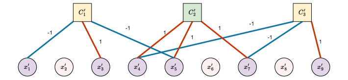
(A)

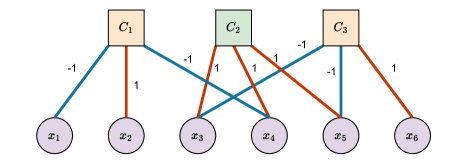
(B)

Figure 3: Instance of 1-in-3 SAT. (A) shows a graphical depiction of an instance of 1-in-3 SAT with 9 variables, $\{x_{1}^{{}^{\prime}},\ldots,x_{9}^{{}^{\prime}}\}$, and 3 clauses. Variables $x_{2}^{{}^{\prime}},x_{6}^{{}^{\prime}},x_{8}^{{}^{\prime}}$ are not used in any clauses and clauses $C_{1}^{\prime}$ and $C_{2}^{\prime}$ form the maximum disjoint set of clauses (MDS) for this problem. (B) shows a graphical depiction of the same instance over the reduced variable space. This specific instance is discussed in Sec. 7.1 as an example of random 1-in-3 SAT instances, in Sec. 7.3 as an instance for which explicit constructions of the initial wavefunction and the mixing operators associated with the MDS are given, and in Sec. 3 as an example of the automated approach to developing the symmetric cover mixer (SymCov).

Given a collection of $m$ clauses, each with $3$ literals, we wish to find an assignment to all $n$ variables such that one and exactly one of the literals in each clause is satisfied. So $1$ literal is satisfied and $2$ are unsatisfied for each clause in the collection. 1-in-3 SAT can be formulated as the following binary linear program (BLP):

$$C^{M}\cdot\vec{x}=\vec{b},\text{ s.t. }C^{M}\in\{-1,0,1\}^{m\times n},b\in\{-2,-1,0,1\}^{m}\text{ and }C^{M}\cdot(1,\ldots,1)=\left\lvert b\right\rvert.$$ (49)

Given a collection of constraints, $\mathcal{C}=\{C_{1},\ldots,C_{m}\}$ with $m=\frac{n}{3}$ and $C_{i}(x)=\sum_{i=j}^{n}c_{ij}x_{j}=1-\sum_{i=j}^{n}(1-c_{ij})/2$ and $\sum_{j=1}^{n}\left\lvert c_{ij}\right\rvert=3$. Then the linear constraint has the form $\vec{c_{i}}\cdot\vec{x}=b_{i}$ for $b_{i}=1-\sum_{i=1}^{n}(1-c_{i})/2$. Then let $C^{M}$ be the row concatenation of $\vec{c_{1}},\ldots,\vec{c_{m}}$ and $\vec{b}=(b_{1},\ldots,b_{m})$.

Then each constraint $C_{i}$ can be associated with a clause, $E_{i}=\{l_{i1},l_{i2},l_{i3}\}$, with literals $l_{ij}=(c_{ij},v_{j})$ such that the polarity $c_{ij}\in\{-1,1\}$ associates $1$ (-1) with a positive literal (negative literal) of the atom and $v_{j}$ is the index of the associated atom (propositional variable) in $X$.

The transition from likely to be satisfiable to likely to be unsatisfiable for random 1-in-k SAT problems occurs with $n/\binom{k}{2}$ clauses [3]. For random 1-in-3 SAT, this occurs with n/3 clauses. To sample from this random distribution, we construct $m=\lceil\frac{n}{3}\rceil$ random clauses such that $c_{ij}\in\{-1,1\}$ uniformly at random over 3 random locations indexed by $j$.

Given that not every variable may participate in the $\lceil\frac{n}{3}\rceil$ clauses, we begin with clauses $C_{i}^{{}^{\prime}}$ over variables $X^{{}^{\prime}}=\{x_{1}^{{}^{\prime}},\ldots,x_{n}^{{}^{\prime}}\}$ and $C_{i}$ is the constraint over the reduced variable space $X=\{x_{1},\ldots,x_{|X|}\}$ by filtering out variables not used (utilizing the unapostrophed definitions for the reduced case keeps the notation cleaner in later sections).

An instance of the 1-in-3 SAT problem is shown in Fig. 3.A with 9 variables, $\{x_{1}^{{}^{\prime}},\ldots,x_{9}^{{}^{\prime}}\}$, and 3 clauses: $C_{1}^{{}^{\prime}}=(-1,0,1,0,-1,0,0,0,0)$, $C_{2}^{{}^{\prime}}=(0,0,0,1,1,0,1,0,0)$, and $C_{3}^{{}^{\prime}}=(0,0,0,-1,0,0,-1,0,1)$. Variables $x_{2}^{{}^{\prime}},x_{6}^{{}^{\prime}},x_{8}^{{}^{\prime}}$ are not used in any clauses. For random instances of 1-in-3 SAT with $\lceil n/3\rceil$ clauses, around the satisfability threshold, it is typical that some varaibles will not be used.

The reduced instance of the problem is represented in Fig. 3.B with $C_{1}=(-1,1,0,-1,0,0)=-1$, $C_{2}=(0,0,1,1,1,0)=1$, $C_{3}=(0,0,-1,0,-1,1)=-1$ and $X=\{x_{1},\ldots,x_{6}\}$. We use this example for explicit constructions of the cost operator Hamiltonian in Sec. 7.2, the maximum disjoint mixer in Sec. 7.3, and the symmetric cover mixer in Sec. 7.3. This instance has two solutions over the reduced variables: $(1,0,0,0,1,0),(1,0,1,0,0,0)$.

7.2 Quantum Approximate Optimization Algorithm for 1-in-3 SAT

Here we describe QAOA with the X-mixer at a high level for 1-in-3 SAT. Let $\sigma^{0}=(1/2)(\mathbbm{1}+\sigma^{z})$, $\sigma^{1}=(1/2)(\mathbbm{1}-\sigma^{z})$, and $\alpha,\beta\in[0,2\pi]^{p}$. Then:

$$U_{p}(\alpha,\beta)=U_{\text{mixer}}(\beta_{p})U_{\text{cost}}(\alpha_{p})\,\ldots\,U_{\text{mixer}}(\beta_{1})\,U_{\text{cost}}(\alpha_{1}).$$ (50)

The cost of a clause, $C_{i}$, is minimized by satisfying one literal and unsatisfying the other literals for 1-in-k SAT:

$$H_{\text{clause}}^{i}=\mathbbm{1}-\sum_{i}\sum_{l_{ij}\in C_{i}}\sigma_{v_{j}}^{(1+c_{ij})/2}\prod_{j\neq i}\sigma_{v_{j}}^{(1-c_{ij})/2}.$$ (51)

For example, consider the example introduced in Sec. 7.3 and depicted in Fig. 3. In this example, $\text{ker}(H_{\text{clause}}^{1})=\text{span}(\{\left\lvert\,0,0,1,x_{4},x_{5},x_{6}\,\right\rangle,\left\lvert\,1,0,0,x_{4},x_{5},x_{6}\,\right\rangle,\left\lvert\,1,1,1,x_{4},x_{5},x_{6}\,\right\rangle\})$, where $x_{4},x_{5},x_{6}\in\{0,1\}$, representing the solution subspace for constraint $C_{1}$.

Then the phase-separating operator, given a specific $\alpha_{l}$, is just:

$$U_{\text{cost}}(\alpha_{l})=\prod_{\text{clause}\in\text{cost}}e^{i\,\alpha_{l}\,H_{\text{clause}}}$$ (52)

Let $|+\rangle_{k}$ represent the plus state over qubit $k$. For the mixing operator, we have the X rotations per qubit for $\beta_{l}$ (written slightly differently than popular as a diffusor):

$$U_{\text{mixer}}(\beta_{l})=\prod_{j=1}^{n}\left(\mathbbm{1}+(e^{-i\,\beta_{l}}-1)|+\rangle_{j}\langle+|_{j}\right).$$ (53)

Notice we place the negative sign for the exponent of the mixing operator and the positive sign for the exponent of the phase-separating operator. The initial wavefunction is:

$$\left\lvert\,\phi(0)\,\right\rangle=\left\lvert\,+\,\right\rangle\ldots\left\lvert\,+\,\right\rangle=\sum_{x\in\{0,1\}^{n}}\frac{1}{\sqrt{2^{n}}}\left\lvert\,x\,\right\rangle$$ (54)

And so the final wavefunction is:

$$\left\lvert\,\phi(p)\,\right\rangle=U_{p}(\alpha,\beta)\left\lvert\,\phi(0)\,\right\rangle$$ (55)

7.3 Maximum Disjoint Clauses and the Quantum Alternating Operator Ansatz

This section details a tailored ansatz approach for solving the 1-in-3 SAT problem using QAOA based on the maximum disjoint set of constraints. When constraints are disjoint, they can be individually solved. Every 1-in-3 SAT clause has precisely 3 solutions out of 8 configurations, just like every 3 SAT clause has precisely 7 solutions out of 8 configurations. The configuration space, $X$, has $2^{n}$ possible configurations, but restricting the space over each constraint in a disjoint set reduces the space by $3/8$. Therefore, given $k$ constraints in the disjoint set, the resulting feasibility constraint space size is $(3/8)^{k}2^{n}$. This section constructs a tailored ansatz utilizing the maximum disjoint set of constraints and Sec. 7.5 supports that this approach can lead to a quadratic advantage for constant depth QAOA optimized with stochastic finite difference descent.

Here we describe the first tailored ansatz for the QAOA on 1-in-3 SAT. Given $m$ linear constraints $\mathcal{C}=\{C_{1},\ldots,C_{m}\}$ over $n$ (reduced) variables $X=\{x_{1},\ldots,x_{n}\}$, we find the maximum disjoint set of constraints (MDS) over the $n$ variables. The MDS is the largest subset of the constraints such that no two constraints share variables (i.e. they are disjoint).

In general, the maximum disjoint set problem is NP-Hard, but in practice over sparse random instances of constraint problems it is tractable in practice. Approximations to the maximum disjoint set problem also exists in the case that finding the maximum disjoint set appears too expensive to compute through standard solvers for integer linear programming. Let $\mathcal{D}=\{C_{D_{1}},\ldots,C_{D_{|\mathcal{D}|}}\}$ be this set. Let $\mathcal{R}=\mathcal{C}-\mathcal{D}$ be the remaining clauses. Let $\mathcal{N}$ be the set of variables not in any constraint in $\mathcal{D}$ (since this is the reduced form of the problem, each variable in $\mathcal{N}$ appears at least once in the remaining clauses $\mathcal{R}$).

For each clause, $C_{D_{i}}$, we find all solutions (there are always three) to define $S_{D}=\{S(C_{D_{1}}),\ldots,S(C_{D_{|D|}})\}$ . Then we associate the uniform superposition density operator for each solution set in $S_{D}$:

$$\hat{S}_{D} =\{\hat{S}(C_{D_{1}}),\ldots,\hat{S}(C_{D_{|D|}})\},$$ (56)

$$\text{where }\hat{S}(C_{D_{i}}) =\frac{1}{\sqrt{3}}\Big{(}\left\lvert\,s_{1}^{i}\,\right\rangle+\left\lvert\,s_{2}^{i}\,\right\rangle+\left\lvert\,s_{3}^{i}\,\right\rangle\Big{)}.$$ (57)

Here each 1-in-3 SAT constraint, $C_{D_{i}}$, in the disjoint set has precisely 3 solutions, $s_{1}^{i},s_{2}^{i},s_{3}^{i}$, over three variables. Hence, each $\hat{S}(C_{D_{i}})$ is a 3-local diffusor. An example based on the 1-in-3 SAT instance visualized in Fig. 3 is described later in this section.

Then the phase-separating operator, given a specific $\alpha_{l}$, is reduced to including constraints in the set $\mathcal{R}$ instead of $\mathcal{C}$:

$$U_{\text{cost}}(\alpha_{l})=\prod_{\text{clause}\in R}e^{i\,\alpha_{l}\,H_{\text{clause}}}$$ (58)

For the mixing operator, we have a diffusor associated with the solutions of each disjoint set in $D$ and a parameter $\beta_{l}$:

$$U_{\text{D}}(\beta_{l},\mathcal{D})=\prod_{\hat{S}(K)\in\hat{S}_{D}}\left(\mathbbm{1}+(e^{-i\,\beta_{l}}-1)\hat{S}(K)\right),$$ (59)

and the ordinary single qubit diffusor ($X$ rotation) on the variables in $\mathcal{N}$:

$$U_{\text{N}}(\beta_{l},\mathcal{N})=\prod_{j\in\mathcal{N}}\left(\mathbbm{1}+(e^{-i\,\beta_{l}}-1)|+\rangle_{j}\langle+|_{j}\right),$$ (60)

Then the overall mixing operator is:

$$U_{\text{mds}}(\beta_{l},\mathcal{C})=U_{\text{D}}(\beta_{l},\mathcal{D})U_{\text{N}}(\beta_{l},\mathcal{N}),$$ (61)

following the construction of Eq. 41.

The initial state is then a uniform superposition overall disjoint clauses, which is easy to prepare.

Consider the instance discussed in Sec. 7.1 and depicted in Fig. 3.B, the MDS is $\{C_{1},C_{3}\}$. The resulting search space is given by $\text{span}(S(C_{1}))\otimes\text{span}(S(C_{3}))=\text{span}(\{\left\lvert\,001\,\right\rangle,\left\lvert\,100\,\right\rangle,\left\lvert\,111\,\right\rangle\}\otimes\{\left\lvert\,010\,\right\rangle,\left\lvert\,100\,\right\rangle,\left\lvert\,111\,\right\rangle\})$. The resulting density operators are:

$$\hat{S}(C_{1}) =\frac{1}{3}\Big{(}\left\lvert\,001\,\right\rangle+\left\lvert\,100\,\right\rangle+\left\lvert\,111\,\right\rangle\Big{)}\Big{(}\left\langle\,001\,\right\rvert+\left\langle\,100\,\right\rvert+\left\langle\,111\,\right\rvert\Big{)}\otimes\mathbbm{1}_{4:6},$$ (62)

$$\hat{S}(C_{3}) =\frac{1}{3}\mathbbm{1}_{1:3}\otimes\Big{(}\left\lvert\,010\,\right\rangle+\left\lvert\,100\,\right\rangle+\left\lvert\,111\,\right\rangle\Big{)}\Big{(}\left\langle\,010\,\right\rvert+\left\langle\,100\,\right\rvert+\left\langle\,111\,\right\rvert\Big{)}.$$ (63)

In this case, $\mathcal{R}=\{C_{2}\}$ and there are no uncovered variables. Then the initial wavefunction is:

$$\left\lvert\,\phi(0)\,\right\rangle=\frac{1}{\sqrt{9}}\Big{(}\left\lvert\,001\,\right\rangle+\left\lvert\,100\,\right\rangle+\left\lvert\,111\,\right\rangle\Big{)}\Big{(}\left\lvert\,010\,\right\rangle+\left\lvert\,100\,\right\rangle+\left\lvert\,111\,\right\rangle\Big{)}.$$ (64)

The mixing operator is:

$$U_{\text{mds}}(\beta,\mathcal{C})=\left(\mathbbm{1}+(e^{-i\beta}-1)\hat{S}(C_{1})\right)\left(\mathbbm{1}+(e^{-i\beta}-1)\hat{S}(C_{3})\right).$$ (65)

The mixing operator written explicitly in the relevant search subspace as a 9$\times$9 matrix:

$\displaystyle\begin{pmatrix}f(\beta)^{2}&f(\beta)g(\beta)&f(\beta)g(\beta)&f(\beta)g(\beta)&g(\beta)^{2}&g(\beta)^{2}&f(\beta)g(\beta)&g(\beta)^{2}&g(\beta)^{2}\\ f(\beta)g(\beta)&f(\beta)^{2}&f(\beta)g(\beta)&g(\beta)^{2}&f(\beta)g(\beta)&g(\beta)^{2}&g(\beta)^{2}&f(\beta)g(\beta)&g(\beta)^{2}\\ f(\beta)g(\beta)&f(\beta)g(\beta)&f(\beta)^{2}&g(\beta)^{2}&g(\beta)^{2}&f(\beta)g(\beta)&g(\beta)^{2}&g(\beta)^{2}&f(\beta)g(\beta)\\ f(\beta)g(\beta)&g(\beta)^{2}&g(\beta)^{2}&f(\beta)^{2}&f(\beta)g(\beta)&f(\beta)g(\beta)&f(\beta)g(\beta)&g(\beta)^{2}&g(\beta)^{2}\\ g(\beta)^{2}&f(\beta)g(\beta)&g(\beta)^{2}&f(\beta)g(\beta)&f(\beta)^{2}&f(\beta)g(\beta)&g(\beta)^{2}&f(\beta)g(\beta)&g(\beta)^{2}\\ g(\beta)^{2}&g(\beta)^{2}&f(\beta)g(\beta)&f(\beta)g(\beta)&f(\beta)g(\beta)&f(\beta)^{2}&g(\beta)^{2}&g(\beta)^{2}&f(\beta)g(\beta)\\ f(\beta)g(\beta)&g(\beta)^{2}&g(\beta)^{2}&f(\beta)g(\beta)&g(\beta)^{2}&g(\beta)^{2}&f(\beta)^{2}&f(\beta)g(\beta)&f(\beta)g(\beta)\\ g(\beta)^{2}&f(\beta)g(\beta)&g(\beta)^{2}&g(\beta)^{2}&f(\beta)g(\beta)&g(\beta)^{2}&f(\beta)g(\beta)&f(\beta)^{2}&f(\beta)g(\beta)\\ g(\beta)^{2}&g(\beta)^{2}&f(\beta)g(\beta)&g(\beta)^{2}&g(\beta)^{2}&f(\beta)g(\beta)&f(\beta)g(\beta)&f(\beta)g(\beta)&f(\beta)^{2}\\ \end{pmatrix},$

with $f(\beta)=(e^{-i\beta}+2)/3$ and $g(\beta)=(e^{-i\beta}-1)/3$.

The cost operator is:

$$U_{\text{cost}}(\alpha,\mathcal{R})=e^{i\alpha H_{C_{2}}}$$ (66)

The cost operator can be written in the search space as a $9\times 9$ matrix:

$$\begin{pmatrix}1&0&0&0&0&0&0&0&0\\ 0&1&0&0&0&0&0&0&0\\ 0&0&1&0&0&0&0&0&0\\ 0&0&0&1&0&0&0&0&0\\ 0&0&0&0&1&0&0&0&0\\ 0&0&0&0&0&1&0&0&0\\ 0&0&0&0&0&0&h(\alpha)&0&0\\ 0&0&0&0&0&0&0&h(\alpha)&0\\ 0&0&0&0&0&0&0&0&1\end{pmatrix},$$

with $h(\alpha)=e^{i\alpha}$.

7.4 Partial and Clause Neighborhood Commutation in the Constraint Graph

Here we describe our third ansatz for QAOA on 1-in-3 SAT, which includes symmetry terms associated with partial constraints as well as between each constraint and the constraints that it shares variables with. Each 1-in-3 SAT clause has 3 (propositional) variables and satisfying conditions associated with each defines the constraints of the problem (Sec. 7.1). The difficulty of satisfying a collection of 1-in-3 SAT clauses, as for all boolean satisfiability problems, arises from the conflicts between a clause and the other clauses that share variables with it since they may have different preferences on what assignments satisfy.

Consider the reduced version of the example 1-in-3 SAT instance introduced in Sec. 7.1, shown in Fig. 3, and discussed in Sec. 7.2 and Sec. 7.3. $C_{1}$ and $C_{2}$ share variables $x_{4}$. Any valid assignment to the 1-in-3 SAT problem must satisfy $C_{1}$ and $C_{2}$, which means the subsets of valid assignments to $C_{1}$ and $C_{2}$ must be compatible, specifically with regard to $x_{4}$. Then it is natural to consider the terms that commute with $C_{1}$ and $C_{2}$, since these terms mixer valid assignments of both $C_{1}$ and $C_{2}$. Similarly, a valid assignment to this example must also be a valid assignment for $C_{2}$ and $C_{3}$, with symmetry terms that mixer the valid assignments of $C_{2}$ and $C_{3}$. Of course, symmetry terms associated with all constraints could be particularly powerful catalyst mixers, but they are unlikely to be local and likely computationally expensive to precompute. By considering a single constraint and the symmetries associated with this particular constraint and those that have at least one variable in common with it, we define terms that mix more constricted assignments even if they do not maintain the global invariance desired. Such mixers, which we call Symmetric Cover (SymCov) mixers, could be applied to many diverse optimization problems characterized by having many local constraints that must be enforced together.

Terms in the MDS could have been found using the flowchart in Fig. 2, but for such simple cases it is not necessary. In this case, we find that higher symmetries, such as the SymCov mixers, are accessible through the approach described in Sec. 6.

For a constraint $C$, we define:

$$S(C)=\{C_{i}\;|\;C_{i}\text{ and }C\text{ share variables}\},$$ (67)

as the neighborhood of $C$.

To construct the Symmetric Cover mixer, the constraints that share variables for each constraint $C$ in the MDS set $\mathcal{D}$ are considered:

$$\mathcal{S}(\mathcal{D})=\{S(C)\,|\,C\in\mathcal{D}\}.$$ (68)

We follow the procedure delineated in Fig. 2, starting with finding all commutative terms $\mathcal{T}(S(C))$ associated with each $S(C)$ in $\mathcal{S}(\mathcal{D})$. Consider a specific $C\in\mathcal{D}$, since the other constraints in the MDS $\mathcal{D}$ by definition have no shared variables, $S(C)\subseteq\mathcal{R}\cup\{C\}$ and $S(C)$ is disjoint from $\mathcal{D}-\{C\}$.

Suppose $3$ constraints in $\mathcal{R}$ are in the neighborhood $S(C)$, then in principle there are more than $2^{55}$ ($12^{12}\times 2^{12}$) possibilities through a brute force method in the worst case, but the backtracking algorithm Alg. 2 from Sec. 6 in practice runs quickly, when implemented with minimal data structures in Julia.

Then, by utilizing Alg. 4 from Sec. 6 we find a collection of generators $\mathcal{G}(S(c))$ from $\mathcal{T}(S(C))$ and a corresponding unitary mixer $U(\gamma,\mathcal{G}(S))$ for each neighborhood $S(C)$ in $\mathcal{S}(\mathcal{D})$. Then the symmetric cover mixer is:

$$U_{\text{symcov}}(\gamma,\mathcal{S})=\prod_{S\in\mathcal{S}}U(\gamma,\mathcal{G}(S)).$$ (69)

Intuitively, the symmetric cover mixer $U(\beta,\mathcal{S})$ acts on the subspace of solutions to the neighborhood $S(C)$ of each constraint $C$ in $\mathcal{D}$, which is strictly smaller than the space of solutions to $\mathcal{D}$. While we considered the unweighted form here, the more general form would have individual optimized angles for each term.

In principle, the subroutine Alg. 3 and therefore Alg. 4 can be exponential time algorithms in the number of generators selected, but we find that in practice Alg. 4 runs quickly for instances up to size $22$.

While the MDS leaves some variables uncovered, we can cover these partially with some of the remaining clauses, although this only leads to a change if there is some constraint with both these terms. Consider a 1-in-3 constraint $C=x_{1}+x_{2}+x_{3}=1$. Suppose $x_{1}$ is covered in the MDS, then $x_{2}+x_{3}\leq 1$ while $x_{1}\leq 1$. Then $(0,0),(1,0),(0,1)$ are possible configurations over $\{x_{2},x_{3}\}$, but not $(1,1)$. Suppose however, $x_{2}$ is also covered in the MDS. Then the only partial constraint we have is $x_{3}\leq 1$, which is identical to no constraint, so we would use the x-mixer. While we will still need to apply penalty terms associated with these clauses, we can apply partial mixers rather than the x-mixer on any constraint with two variables outside the MDS. Let $U_{R}(\beta,\mathcal{R})$ refer to this approach and $U_{mds}(\beta,\mathcal{C})=U_{D}(\beta,\mathcal{D})U_{R}(\beta,\mathcal{R})$.

Then one round of generalized QAOA is:

$$\left\lvert\,\psi_{p}\,\right\rangle=U_{\text{symcov}}(\gamma,\mathcal{S}(\mathcal{D}))\;U_{\text{mds}}(\beta,\mathcal{C})\;U_{\text{cost}}(\alpha,\mathcal{R})\left\lvert\,\psi_{p-1}\,\right\rangle$$ (70)

The generic algorithms presented in Sec. 6 can be used in many constructions, and their use in this section is only an example of their utility. While considered in the context of 1-in-3 SAT, similar constructions as the symmetric cover disccused in this Section could be applied to most feasibility or optimization problems that have local constraints. Even if the constraints are not local, Alg. 2 can be utilized for finding local terms up to a desired weight.

7.5 Benchmarks and Scaling Extrapolation

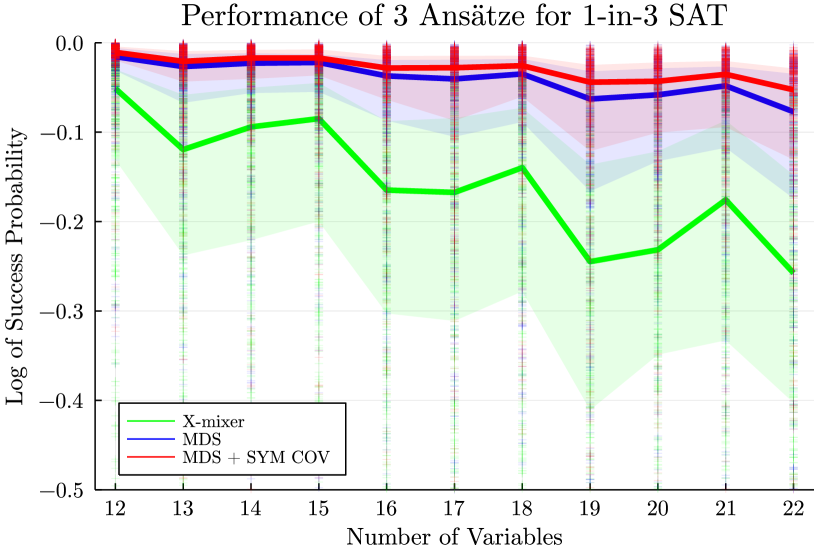
Figure 4: Ansatz Benchmarks for 1-in-3 SAT. The success probability versus number of variables in the random instance of the 1-in-3 SAT problem with sizes between $12$ and $22$. The green QAOA with x-mixer (blue QAOA with MDS mixer, red QAOA with MDS+SYMCOV) dots show the success probability after $14$ rounds of QAOA on each instance while the green (blue, red) line is the median surrounded by the upper and lower quartile ribbon on $500$ random satisfiable instances for each size.

	cofactor	exponent base
X mixers	0.8973	1.0209
MDS mixers	0.9193	1.0107
MDS+SymCov mixers	0.9256	1.0092

Table 2: Exponential Curve Fits for each Ansatz. We fit exponential curves $f(n)=AB^{n}$, with cofactor $A$ and exponent base $B$ using a package to minimize the mean squared error for problem size $n$ and empirical inverse success probability as shown in Fig. 4. The low exponent for each approach suggests QAOA is well suited for solving 1-in-k SAT problems and that tailored ansätze can improve QAOA’s relative performance, with an empirical performance gain associated with a superpolynomial (quadratic) advantage.

We benchmark QAOA with x-mixer, MDS mixer, and MDS mixer plus symmetric cover mixer with $p=14$ from size $12$ and $22$ over $500$ random instances drawn with $n/3$ clauses and $3$ variables per clause, with each clause generated by selecting three variables in the range $[1,n]$ at random and the polarity of the literal (negative or positive) selected with even probability. Resulting instances with no solution are discarded and the process is repeated until $500$ satisfiable instances are generated in total.

With instances of size $12$, we optimize the collections of angles $\alpha,\beta$ of each approach in two rounds for p set to $14$. We sweep over different starting values for overall coefficient $a$ and $b$ (10 each) and two choices for the function associated each vector: constant $\alpha=(a,\ldots,a,a),\beta=(b,\ldots,b)$ and linear $\alpha=(a/p,\ldots,a(p-1)/p,a),\beta=(b,\ldots,2b/p,b/p)$. After a few steps, we find that sweeping between $[0.0,0.2]$ for $\alpha$ and $[0.0,0.05]$ for $\beta$ with 100 individual initialization considered in the grid search for each choice (constant or linear). For each sweep, we do $5000$ rounds of finite difference gradient descent, then take the best result and run $50000$ rounds of gradient descent to further optimize the angles. For the third approach, MDS+SymCov described by Eq. 70, we then do $50000$ rounds of gradient descent over the collection of angles $\alpha,\beta,\gamma$ starting with $\gamma=\mathbf{0}$ (all zeros vector). Intuitively, $U_{\text{symcov}}(\gamma,\mathcal{S}(\mathcal{D}))$ acts as a catalyst.

In Fig. 4, results for each approach is shown with the median performance shown as a solid line and ribbons depicting the upper and lower quartiles. The results are consistent with better overall performance for the mds mixer in comparison to the x mixer and the strongesst performance for the mds mixer with the symmetric cover mixer. We use CurveFit.jl to optimize the mean-squared loss of fitting an exponential curve $A\,B^{x}$ for values of $A$ and $B$. The results are summarized in Tab. 2, with a quadratic advantage (e.g. $1.0092^{2.25}\approx 1.0209$) in the exponent for the advanced mixers. Our $p=14$ results show strong performance from all approaches and a soft decay for larger size $n$, suggesting that QAOA may be well suited for solving 1-in-k SAT just as it has seen utility for k-SAT in Ref. [37]. However, results in this work suggest that if the Quantum Approximate Optimization Algorithm (QAOA with the x-mixer) is able to achieve a form of quantum advantage, a better suited ansatz could dramatically enhance that advantage.

8 Conclusion and Outlook

In this manuscript, we discuss the algebraic and algorithmic foundations of imposing constraints on quantum operators, focusing on the utilization of such operators to aide new ansatz constructions and clarify the complexity of such related tasks. Ansatz construction can aide in improved success probability [41], reduced expressability [23, 25, 33], learnability [40], and noise resistance [36]. Our results support that symmetry terms can aide as catalysts in QAOA as well as significantly reduce the search space, thereby improving the success probability.

Finding commutative terms for embedded constraints is in general NP-Complete, but is polynomial for locally bounded constraints in the degree of the bound (Sec. 4). Sec. 6 provides practical algorithmic procedures that can solve the problem in formidable run-times despite the high upper bound. Along the way (see Fig. 2), we clarify important points of consideration for practical ansatz construction, such as grouping commutative terms (Sec. 5 and Sec. 6.2) and defining unitary operators (Sec. 6.3).

Such algorithms can be useful for constructing driver Hamiltonians or unitary mixers for a large array of optimization problems, while the reformulations, such as in App. A, can be geared towards native quantum tasks for quantum computers to solve.

In Ref. [32], it was shown that any 2-local Hamiltonian nonviable for certain classes of constraints. The algebraic condition found in this manuscript can also be utilized to find similar exclusionary statements for problems using more general constraints, thereby showing that certain constructions are not viable under resource restrictions.

This work presents many avenues for future study. While the problem CP-QIRREDUCIBLE-COMMUTE is NP-Hard, a more precise statement about its complexity within the polynomial hierarchy is an open problem, as well as the same problem for linear constraints. Coefficients $\alpha$ on commutative terms $T$ can be any complex number, thereby including nonstoquastic Hamiltonian drivers and their associated mixers. A satisfactory mathematical framework that allows us to select these coefficients or general learning techinques to find optimal patterns is of clear interest. Finding practical problems in quantum chemistry for which the expressions found in App. A provide a useful secondary ansatz or catalyst driver term is another exciting avenue. They could also be used for error suppression techniques.

While Alg. 2 for finding commutative terms is exact, alternative primitives may offer better runtime guarantees with good approximation and wider applicability. Alg. 4 is a simple practical approximation algorithm; alternative algorithmic primitives to sequencing generators into unitary mixers could improve practical circuit depth or perform better based on other criteria. Developing special purpose transpilers for mapping generators to low-body gates with limited connectivity can be a useful avenue for future consideration to apply these techniques to current NISQ hardware. Beyond this future work can consider suitable constructions for still wider varieties of problems, constraints, and encodings, including integer problems and qudit-based mixers constructions suitable for qudits [48].

Appendix A Sufficient Conditions for Quadratic Constraints

Given any complete basis for a single qubit system, we can extend that basis to define a basis over $n$ qubits. As discussed in previous sections $\sigma^{+}=\left\lvert\,1\,\right\rangle\!\left\langle\,0\,\right\rvert$ and $\sigma^{-}=\left\lvert\,0\,\right\rangle\!\left\langle\,1\,\right\rvert$. Then we can utilize the complete basis $\{\mathbbm{1},\sigma^{z},\sigma^{+},\sigma^{-}\}^{\otimes n}$. Note that $\left(\alpha_{j}\sigma_{i}^{\pm}\right)^{\dagger}=\alpha_{j}^{\dagger}\sigma_{i}^{\mp}$ for $\alpha_{j}\in\mathbb{C}$. Then any Hermitian matrix can be written in the form:

$$H =\sum_{(\vec{y_{j}},\vec{v_{j}},\vec{w_{j}})\in\Delta(\mathscr{Y},\;\mathscr{V},\;\mathscr{W})}\alpha_{j}\prod_{i=1}^{n}\left(\sigma^{z}\right)^{y_{ji}}\left(\sigma^{+}\right)^{v_{ji}}\left(\sigma^{-}\right)^{w_{ji}}$$

$$\phantom{=}+\sum_{(\vec{y_{j}},\vec{v_{j}},\vec{w_{j}})\in\Delta(\mathscr{Y},\;\mathscr{V},\;\mathscr{W})}\alpha_{j}^{\dagger}\prod_{i=1}^{n}\left(\sigma^{z}\right)^{y_{ji}}\left(\sigma^{+}\right)^{w_{ji}}\left(\sigma^{-}\right)^{v_{ji}},$$ (71)

Recall the main algebraic result from Ref. [32]:

Theorem A.1 (Algebraic Condition for Commutativity).

A Hermitian Matrix $H$ commutes with an embedding of a linear constraint $C$ if and only if $\vec{c}\cdot(\vec{v}_{j}-\vec{w}_{j})=0$ for all $\vec{v}_{j},\vec{w}_{j}\in\Delta(\mathscr{V},\mathscr{W})$.

In this paper, we wish to find similar algebraic conditions for more general constraints. For higher term constraints, we can write the constraint in the general form:

$$\hat{C}=\sum_{J_{K}\in\mathcal{J}}J_{K}\prod_{k\in K}\sigma_{k}^{z},$$ (72)

where $\mathcal{J}$ is a collection of sets of polynomial size in the number of qubits $n$, each with a coefficient $J_{K}$ and a set of qubit indices $K\subseteq[1,\ldots,n]$. Notice that $\sigma^{+}\sigma^{z}=-\sigma^{z}\sigma^{+}=\sigma^{+}$ and $\sigma^{-}\sigma^{z}=-\sigma^{z}\sigma^{-}=-\sigma^{-}$.

Using the form for $H$ from Eq. 71, define $T(\vec{y},\vec{v},\vec{w})=\prod_{i=1}^{n}\left(\sigma_{i}^{z}\right)^{y_{i}}\left(\sigma_{i}^{+}\right)^{v_{i}}\left(\sigma_{i}^{-}\right)^{w_{i}}$ such that $T^{\dagger}(\vec{y},\vec{v},\vec{w})=T(\vec{y},\vec{w},\vec{v})$.

Then consider the commutation of a general $H$ with the constraint embedding operator for a general constraint $C$:

$$\left[H,\hat{C}\right] =\sum_{(\vec{y_{j}},\vec{v_{j}},\vec{w_{j}})\in\Delta(\mathscr{Y},\;\mathscr{V},\;\mathscr{W})}\left[\alpha_{j}\prod_{i=1}^{n}\left(\sigma_{i}^{z}\right)^{y_{ji}}\left(\sigma_{i}^{+}\right)^{v_{ji}}\left(\sigma_{i}^{-}\right)^{w_{ji}},\sum_{J_{K}\in\mathcal{J}}J_{K}\prod_{k\in K}\sigma_{k}^{z}\right]$$

$$\phantom{=}+\sum_{(\vec{y_{j}},\vec{v_{j}},\vec{w_{j}})\in\Delta(\mathscr{Y},\;\mathscr{V},\;\mathscr{W})}\left[\alpha_{j}^{\dagger}\prod_{i=1}^{n}\left(\sigma_{i}^{z}\right)^{y_{ji}}\left(\sigma_{i}^{+}\right)^{w_{ji}}\left(\sigma_{i}^{-}\right)^{v_{ji}},\sum_{J_{K}\in\mathcal{J}}J_{K}\,\prod_{k\in K}\sigma_{k}^{z}\right]$$

$$=\sum_{(\vec{y_{j}},\vec{v_{j}},\vec{w_{j}})\in\Delta(\mathscr{Y},\;\mathscr{V},\;\mathscr{W})}\alpha_{j}\,\sum_{J_{K}\in\mathcal{J}}J_{K}\,L_{jK}$$

$$\phantom{=}+\sum_{(\vec{y_{j}},\vec{v_{j}},\vec{w_{j}})\in\Delta(\mathscr{Y},\;\mathscr{V},\;\mathscr{W})}\alpha_{j}^{\dagger}\,\sum_{J_{K}\in\mathcal{J}}J_{K}\,R_{jK}$$ (73)

where:

$$L_{jK} =\left(\prod_{k\notin K}\left(\sigma_{k}^{z}\right)^{y_{jk}}\left(\sigma_{k}^{+}\right)^{w_{jk}}\left(\sigma_{k}^{-}\right)^{v_{jk}}\right)\left[\prod_{k\in K}\left(\sigma_{k}^{z}\right)^{y_{jk}}\left(\sigma_{k}^{+}\right)^{w_{jk}}\left(\sigma_{k}^{-}\right)^{v_{jk}},\prod_{k\in k}\sigma_{k}^{z}\right]$$

$$=\left(\prod_{k\notin K}\left(\sigma_{k}^{z}\right)^{y_{jk}}\left(\sigma_{k}^{+}\right)^{w_{jk}}\left(\sigma_{k}^{-}\right)^{v_{jk}}\right)\,\left(\prod_{k\in K}\left(\sigma_{k}^{z}\right)^{y_{jk}}\left(\sigma_{k}^{+}\right)^{w_{jk}}\left(\sigma_{k}^{-}\right)^{v_{jk}}\sigma_{k}^{z}-\prod_{k\in K}\sigma_{k}^{z}\left(\sigma_{k}^{z}\right)^{y_{jk}}\left(\sigma_{k}^{+}\right)^{w_{jk}}\left(\sigma_{k}^{-}\right)^{v_{jk}}\right)$$

$$=\left(\prod_{k\notin K}\left(\sigma_{k}^{z}\right)^{y_{jk}}\left(\sigma_{k}^{+}\right)^{w_{jk}}\left(\sigma_{k}^{-}\right)^{v_{jk}}\right)\,\prod_{k\in K}(-1)^{v_{jk}}\left(\sigma_{k}^{z}\right)^{y_{jk}+\mu_{jk}}\left(\sigma_{k}^{+}\right)^{w_{jk}}\left(\sigma_{k}^{-}\right)^{v_{jk}}$$

$$\phantom{=}-\left(\prod_{k\notin K}\left(\sigma_{k}^{z}\right)^{y_{jk}}\left(\sigma_{k}^{+}\right)^{w_{jk}}\left(\sigma_{k}^{-}\right)^{v_{jk}}\right)\prod_{k\in K}(-1)^{w_{jk}}\left(\sigma_{k}^{z}\right)^{y_{jk}+\mu_{jk}}\left(\sigma_{k}^{+}\right)^{w_{jk}}\left(\sigma_{k}^{-}\right)^{v_{jk}}$$

$$=\left(\prod_{k\in K}(-1)^{v_{jk}}-(-1)^{w_{jk}}\right)\prod_{k\in K}\left(\sigma_{k}^{z}\right)^{\mu_{jk}}\,T(\vec{y_{j}},\vec{v_{j}},\vec{w_{j}})$$

$$=2^{|K|}\;\left(\prod_{k\in K}v_{jk}-w_{jk}\right)T(\vec{y_{j}}+\vec{\mu_{j}},\vec{v_{j}},\vec{w_{j}})$$ (74)

with $\mu_{jk}=(1-v_{jk})(1-w_{jk})$ (identity or spin-z were placed on location $k$ by the $j$-th basis term), and so $\vec{\mu_{j}}=(\mu_{j1},\ldots,\mu_{jn})$. Likewise, it can be shown:

$$R_{jK}=2^{|K|}\;\left(\prod_{k\in K}w_{jk}-v_{jk}\right)T(\vec{y_{j}}+\vec{\mu_{j}},\vec{w_{j}},\vec{v_{j}})$$ (75)

and so:

$$\left[H,\hat{C}\right] =\phantom{+}\sum_{(\vec{y_{j}},\vec{v_{j}},\vec{w_{j}})\in\Delta(\mathscr{Y},\;\mathscr{V},\;\mathscr{W})}\alpha_{j}\,\sum_{J_{K}\in\mathcal{J}}J_{K}\,2^{|K|}\left(\prod_{k\in K}v_{jk}-w_{jk}\right)T(\vec{y_{j}}+\vec{\mu_{j}},\vec{v_{j}},\vec{w_{j}})$$

$$\phantom{=}+\sum_{(\vec{y_{j}},\vec{v_{j}},\vec{w_{j}})\in\Delta(\mathscr{Y},\;\mathscr{V},\;\mathscr{W})}\alpha_{j}^{\dagger}\,\sum_{J_{K}\in\mathcal{J}}J_{K}\,2^{|K|}\left(\prod_{k\in K}w_{jk}-v_{jk}\right)T(\vec{y_{j}}+\vec{\mu_{j}},\vec{w_{j}},\vec{v_{j}})$$

$$=\phantom{+}\sum_{(\vec{y_{j}},\vec{v_{j}},\vec{w_{j}})\in\Delta(\mathscr{Y},\;\mathscr{V},\;\mathscr{W})}\alpha_{j}\,\sum_{J_{K}\in\mathcal{J}}J_{K}\,2^{|K|}\left(\prod_{k\in K}u_{jk}\right)T(\vec{y_{j}}+\vec{\mu_{j}},\vec{v_{j}},\vec{w_{j}})$$

$$\phantom{=}+\sum_{(\vec{y_{j}},\vec{v_{j}},\vec{w_{j}})\in\Delta(\mathscr{Y},\;\mathscr{V},\;\mathscr{W})}\alpha_{j}^{\dagger}\,\sum_{J_{K}\in\mathcal{J}}J_{K}\,2^{|K|}\left(\prod_{k\in K}-u_{jk}\right)T(\vec{y_{j}}+\vec{\mu_{j}},\vec{w_{j}},\vec{v_{j}}).$$ (76)

Define $v(\mathcal{J},\mathcal{Y},\mathcal{V},\mathcal{W})\in\mathbb{C}^{2^{3n}}$, which appears like Eq. 76 except $T(\vec{y},\vec{v},\vec{w})$ is replaced by $\vec{y}\otimes\vec{v}\otimes\vec{w}$. Clearly Eq. 76 is zero if and only if $v(\mathcal{J},\mathcal{Y},\mathcal{V},\mathcal{W})=0$. We can define $u_{j}=\vec{v_{j}}-\vec{w_{j}}$ since $\vec{v_{j}},\vec{w_{j}}$ never match on an index.

Given that $H$ has $\mathcal{O}\left(\text{poly}(n)\right)$ nonzero terms over the basis, there are at most $\mathcal{O}\left(|\mathcal{J}|\,\text{poly}(n)\right)$ such terms to check, all of which must be zero.

A class of constraints of particular interest are quadratic constraints, which can be used to describe a large class of optimization problems. Certain NP-Hard problems, for example, are more naturally described with quadratic constraints. In this section we give a sufficient condition for quadratic constraints that generalizes naturally from Theorem A.1.

Let us check that Eq. 76 matches our result from Theorem A.1 when considering linear constraints, i.e. $\hat{C}=\sum_{k=1}^{n}J_{k}\sigma_{k}^{z}$:

$$\left[H,\hat{C}\right] =\phantom{+}\sum_{(\vec{y_{j}},\vec{v_{j}},\vec{w_{j}})\in\Delta(\mathscr{Y},\;\mathscr{V},\;\mathscr{W})}\alpha_{j}\,\sum_{J_{K}\in\mathcal{J}}J_{K}\,2^{|K|}\left(\prod_{k\in K}v_{jk}-w_{jk}\right)T(\vec{y_{j}}+\vec{\mu_{j}},\vec{v_{j}},\vec{w_{j}})$$

$$\phantom{=}+\sum_{(\vec{y_{j}},\vec{v_{j}},\vec{w_{j}})\in\Delta(\mathscr{Y},\;\mathscr{V},\;\mathscr{W})}\alpha_{j}^{\dagger}\,\sum_{J_{K}\in\mathcal{J}}J_{K}\,2^{|K|}\left(\prod_{k\in K}w_{jk}-v_{jk}\right)T(\vec{y_{j}}+\vec{\mu_{j}},\vec{w_{j}},\vec{v_{j}})$$

$$=\phantom{+}2\,\sum_{(\vec{y_{j}},\vec{v_{j}},\vec{w_{j}})\in\Delta(\mathscr{Y},\;\mathscr{V},\;\mathscr{W})}\alpha_{j}\sum_{k=1}^{n}J_{k}\left(v_{jk}-w_{jk}\right)T(\vec{y_{j}},\vec{w_{j}},\vec{v_{j}})$$

$$\phantom{=}+2\,\sum_{(\vec{y_{j}},\vec{v_{j}},\vec{w_{j}})\in\Delta(\mathscr{Y},\;\mathscr{V},\;\mathscr{W})}\alpha_{j}^{\dagger}\sum_{k=1}^{n}J_{k}\left(w_{jk}-v_{jk}\right)T(\vec{y_{j}},\vec{w_{j}},\vec{v_{j}})$$

$$=\phantom{+}2\,\sum_{(\vec{y_{j}},\vec{v_{j}},\vec{w_{j}})\in\Delta(\mathscr{Y},\;\mathscr{V},\;\mathscr{W})}\alpha_{j}\,\vec{J}\cdot\left(\vec{v_{j}}-\vec{w_{j}}\right)T(\vec{y_{j}},\vec{w_{j}},\vec{v_{j}})$$

$$\phantom{=}-2\,\sum_{(\vec{y_{j}},\vec{v_{j}},\vec{w_{j}})\in\Delta(\mathscr{Y},\;\mathscr{V},\;\mathscr{W})}\alpha_{j}^{\dagger}\,\vec{J}\cdot\left(\vec{v_{j}}-\vec{w_{j}}\right)T(\vec{y_{j}},\vec{w_{j}},\vec{v_{j}})$$ (77)

Now, let us consider the case with quadratic and linear terms in the constraint. For such a constraint, the constraint embedding operator has the form $\hat{C}=\sum_{i}h_{i}\sigma_{i}^{z}+\sum_{ij}J_{ij}\sigma_{i}^{z}\sigma_{j}^{z}$ and so:

$$\left[H,\hat{C}\right] =\phantom{+}\sum_{(\vec{y_{j}},\vec{v_{j}},\vec{w_{j}})\in\Delta(\mathscr{Y},\;\mathscr{V},\;\mathscr{W})}\alpha_{j}\,\sum_{J_{K}\in\mathcal{J}}J_{K}\,2^{|K|}\left(\prod_{k\in K}v_{jk}-w_{jk}\right)T(\vec{y_{j}}+\vec{\mu_{j}},\vec{v_{j}},\vec{w_{j}})$$

$$\phantom{=}+\sum_{(\vec{y_{j}},\vec{v_{j}},\vec{w_{j}})\in\Delta(\mathscr{Y},\;\mathscr{V},\;\mathscr{W})}\alpha_{j}^{\dagger}\,\sum_{J_{K}\in\mathcal{J}}J_{K}\,2^{|K|}\left(\prod_{k\in K}w_{jk}-v_{jk}\right)T(\vec{y_{j}}+\vec{\mu_{j}},\vec{w_{j}},\vec{v_{j}})$$

$$=\phantom{+}2\,\sum_{(\vec{y_{j}},\vec{v_{j}},\vec{w_{j}})\in\Delta(\mathscr{Y},\;\mathscr{V},\;\mathscr{W})}\alpha_{j}\sum_{k=1}^{n}h_{k}\left(v_{jk}-w_{jk}\right)T(\vec{y_{j}},\vec{w_{j}},\vec{v_{j}})$$

$$\phantom{=}+2\,\sum_{(\vec{y_{j}},\vec{v_{j}},\vec{w_{j}})\in\Delta(\mathscr{Y},\;\mathscr{V},\;\mathscr{W})}\alpha_{j}^{\dagger}\sum_{k=1}^{n}h_{k}\left(w_{jk}-v_{jk}\right)T(\vec{y_{j}},\vec{w_{j}},\vec{v_{j}})$$

$$\phantom{=}+4\,\sum_{(\vec{y_{j}},\vec{v_{j}},\vec{w_{j}})\in\Delta(\mathscr{Y},\;\mathscr{V},\;\mathscr{W})}\alpha_{j}\sum_{kl}J_{kl}\left(v_{jk}-w_{jk}\right)\left(v_{jl}-w_{jl}\right)\left(\sigma_{k}^{z}\right)^{\mu_{jk}}\left(\sigma_{l}^{z}\right)^{\mu_{jl}}T(\vec{y_{j}},\vec{w_{j}},\vec{v_{j}})$$

$$\phantom{=}+4\,\sum_{(\vec{y_{j}},\vec{v_{j}},\vec{w_{j}})\in\Delta(\mathscr{Y},\;\mathscr{V},\;\mathscr{W})}\alpha_{j}^{\dagger}\sum_{kl}^{n}J_{kl}\left(w_{jk}-v_{jk}\right)\left(w_{jl}-v_{jl}\right)\left(\sigma_{k}^{z}\right)^{\mu_{jk}}\left(\sigma_{l}^{z}\right)^{\mu_{jl}}T(\vec{y_{j}},\vec{w_{j}},\vec{v_{j}})$$ (78)

To get a sufficient condition, assume terms associated with $\{h_{i}\}$ and $\{J_{ij}\}$ are zero respectively. The first condition is the previous result $\vec{h}\cdot\left(\vec{v_{j}}-\vec{w_{j}}\right)=\vec{h}\cdot\vec{u_{j}}=0$. A sufficient condition on the second is $\sum_{kl}J_{kl}\left(v_{jk}-w_{jk}\right)\left(v_{jl}-w_{jl}\right)=\sum_{kl}J_{kl}u_{jk}u_{jl}=\vec{u_{j}}^{T}\cdot J^{M}\cdot\vec{u_{j}}=0$.

Theorem A.2 (Sufficient Condition for Quadratic).

A Hermitian Matrix $H$ commutes with an embedding of a quadratic constraint $C$ if $\vec{h}\cdot\vec{u}_{j}=0$ and $\vec{u}_{j}^{T}\cdot J^{M}\cdot\vec{u}_{j}=0$ for all $\vec{u}_{j}$.

While this condition is sufficient, it is not necessary for $H$ to commute with the constraint embedding operator. We consider a simple concrete counterexample. Consider constraints associated with the maximum independent set problem, where we wish to maximize a set of vertices $S\subseteq V$ such that no $v\in S$ has an edge to any other $w\in S$. This can be represented with the quadratic constraints:

$$\forall v\in V,\;\sum_{(v,w)\in E}x_{v}\,x_{w}=0.$$ (79)

Clearly the Hamiltonian $(\sigma_{v}^{+}+\sigma^{-}\prod_{(v,w)\in E}\sigma_{w}^{0}=\left(\sigma_{v}^{+}+\sigma_{v}^{-}\right)\prod_{(v,w)\in E}\left(\mathbbm{1}+\sigma_{w}^{z}\right)$ commutes with the embedded constraint, but does not satisfy this sufficient condition (see Sec. 3). Let us consider the case with $C=\left(\mathbbm{1}-\sigma_{1}^{z}\right)\left(\mathbbm{1}-\sigma_{2}^{z}\right)=\mathbbm{1}-\sigma_{1}^{z}-\sigma_{2}^{z}+\sigma_{1}^{z}\sigma_{1}^{z}$. Note that the expressions found in Sec. 3 are more useful for this case, since $\sigma^{0}$ and $\sigma^{1}$ are more naturally expressed in that formulation.

Appendix B Multiplication Tables for Single Qubit Operators

B.1 For the Operators $\{\mathbbm{1},\sigma^{0},\sigma^{1},\sigma^{-},\sigma^{+}\}$

Relevant to results derived in Sec. 3 and Sec. 5 are multiplication identities for the single qubit operators $\sigma^{0}=\left\lvert\,0\,\right\rangle\!\left\langle\,0\,\right\rvert,\sigma^{1}=\left\lvert\,1\,\right\rangle\!\left\langle\,1\,\right\rvert,\sigma^{+}=\left\lvert\,1\,\right\rangle\!\left\langle\,0\,\right\rvert,\sigma^{-}=\left\lvert\,0\,\right\rangle\!\left\langle\,1\,\right\rvert$. Here we list the left-multiplication and right-multiplication identities for each matrix.

$$\sigma^{0}$$ left

$$\sigma^{0}\sigma^{0} =\sigma^{0}$$

$$\sigma^{0}\sigma^{1} =0$$

$$\sigma^{0}\sigma^{-} =\sigma^{-}$$

$$\sigma^{0}\sigma^{+} =0$$

$$\sigma^{0}\left(\sigma^{0}\right)^{x}\left(\sigma^{1}\right)^{y}\left(\sigma^{+}\right)^{v}\left(\sigma^{-}\right)^{w} =\left(1-\Theta(y+v)\right)\left(\sigma^{0}\right)^{x}\left(\sigma^{1}\right)^{y}\left(\sigma^{+}\right)^{v}\left(\sigma^{-}\right)^{w}$$

$$\sigma^{0}$$ right

$$\sigma^{0}\sigma^{0} =\sigma^{0}$$

$$\sigma^{1}\sigma^{0} =0$$

$$\sigma^{-}\sigma^{0} =0$$

$$\sigma^{+}\sigma^{0} =\sigma^{+}$$

$$\left(\sigma^{0}\right)^{x}\left(\sigma^{1}\right)^{y}\left(\sigma^{+}\right)^{v}\left(\sigma^{-}\right)^{w}\sigma^{0} =\left(1-\Theta(y+w)\right)\left(\sigma^{0}\right)^{x}\left(\sigma^{1}\right)^{y}\left(\sigma^{+}\right)^{v}\left(\sigma^{-}\right)^{w}$$ (80)

$$\sigma^{1}$$ left

$$\sigma^{1}\sigma^{0} =0$$

$$\sigma^{1}\sigma^{1} =\sigma^{1}$$

$$\sigma^{1}\sigma^{-} =0$$

$$\sigma^{1}\sigma^{+} =\sigma^{+}$$

$$\sigma^{1}\left(\sigma^{0}\right)^{x}\left(\sigma^{1}\right)^{y}\left(\sigma^{+}\right)^{v}\left(\sigma^{-}\right)^{w} =\left(1-\Theta(x+w)\right)\left(\sigma^{0}\right)^{x}\left(\sigma^{1}\right)^{y}\left(\sigma^{+}\right)^{v}\left(\sigma^{-}\right)^{w}$$

$$\sigma^{1}$$ right

$$\sigma^{0}\sigma^{1} =0$$

$$\sigma^{1}\sigma^{1} =\sigma^{1}$$

$$\sigma^{-}\sigma^{1} =\sigma^{-}$$

$$\sigma^{+}\sigma^{1} =0$$

$$\left(\sigma^{0}\right)^{x}\left(\sigma^{1}\right)^{y}\left(\sigma^{+}\right)^{v}\left(\sigma^{-}\right)^{w}\sigma^{1} =\left(1-\Theta(x+v)\right)\left(\sigma^{0}\right)^{x}\left(\sigma^{1}\right)^{y}\left(\sigma^{+}\right)^{v}\left(\sigma^{-}\right)^{w}$$

$$\sigma^{+}$$ left

$$\sigma^{+}\sigma^{0} =\sigma^{+}$$

$$\sigma^{+}\sigma^{1} =0$$

$$\sigma^{+}\sigma^{-} =\sigma^{1}$$

$$\sigma^{+}\sigma^{+} =0$$

$$\sigma^{+}\left(\sigma^{0}\right)^{x}\left(\sigma^{1}\right)^{y}\left(\sigma^{+}\right)^{v}\left(\sigma^{-}\right)^{w} =\left(1-\Theta(y+v)\right)\left(\sigma^{0}\right)^{x}\left(\sigma^{1}\right)^{y+w}\left(\sigma^{+}\right)^{v}$$

$$\sigma^{+}$$ right

$$\sigma^{0}\sigma^{+} =0$$

$$\sigma^{1}\sigma^{+} =\sigma^{+}$$

$$\sigma^{-}\sigma^{+} =\sigma^{0}$$

$$\sigma^{+}\sigma^{+} =0$$

$$\left(\sigma^{0}\right)^{x}\left(\sigma^{1}\right)^{y}\left(\sigma^{+}\right)^{v}\left(\sigma^{-}\right)^{w}\sigma^{+} =\left(1-\Theta(x+v)\right)\left(\sigma^{0}\right)^{x+w}\left(\sigma^{1}\right)^{y}\left(\sigma^{+}\right)^{v}$$

$$\sigma^{-}$$ left

$$\sigma^{-}\sigma^{0} =0$$

$$\sigma^{-}\sigma^{1} =\sigma^{-}$$

$$\sigma^{-}\sigma^{-} =0$$

$$\sigma^{-}\sigma^{+} =\sigma^{0}$$

$$\sigma^{-}\left(\sigma^{0}\right)^{x}\left(\sigma^{1}\right)^{y}\left(\sigma^{+}\right)^{v}\left(\sigma^{-}\right)^{w} =\left(1-\Theta(x+w)\right)\left(\sigma^{0}\right)^{x+v}\left(\sigma^{1}\right)^{y}\left(\sigma^{+}\right)^{v}\left(\sigma^{-}\right)^{w}$$

$$\sigma^{-}$$ right

$$\sigma^{0}\sigma^{-} =\sigma^{-}$$

$$\sigma^{1}\sigma^{-} =0$$

$$\sigma^{-}\sigma^{-} =0$$

$$\sigma^{+}\sigma^{-} =\sigma^{1}$$

$$\left(\sigma^{0}\right)^{x}\left(\sigma^{1}\right)^{y}\left(\sigma^{+}\right)^{v}\left(\sigma^{-}\right)^{w}\sigma^{-} =\left(1-\Theta(y+w)\right)\left(\sigma^{0}\right)^{x}\left(\sigma^{1}\right)^{y+v}\left(\sigma^{+}\right)^{v}\left(\sigma^{-}\right)^{w}$$

B.2 For the Operators $\{\mathbbm{1},\sigma^{z},\sigma^{-},\sigma^{+}\}$

Relevant to results derived in App. A are multiplication identities for the single qubit operators $\mathbbm{1},\sigma^{z}=\left\lvert\,0\,\right\rangle\!\left\langle\,0\,\right\rvert-\left\lvert\,1\,\right\rangle\!\left\langle\,1\,\right\rvert,\sigma^{+}=\left\lvert\,1\,\right\rangle\!\left\langle\,0\,\right\rvert,\sigma^{-}=\left\lvert\,0\,\right\rangle\!\left\langle\,1\,\right\rvert$. Here we list the left-multiplication and right-multiplication identities for each matrix.

$$\sigma^{z}$$ left

$$\sigma^{z}\sigma^{z} =\mathbbm{1}$$

$$\sigma^{z}\sigma^{-} =\sigma^{-}$$

$$\sigma^{z}\sigma^{+} =-\sigma^{+}$$

$$\sigma^{z}\left(\sigma^{z}\right)^{x}\left(\sigma^{+}\right)^{v}\left(\sigma^{-}\right)^{w} =\left(-1\right)^{v}\left(\sigma^{+}\right)^{v}\left(\sigma^{-}\right)^{w}$$

$$\sigma^{z}$$ right

$$\sigma^{z}\sigma^{z} =\mathbbm{1}$$

$$\sigma^{-}\sigma^{z} =-\sigma^{-}$$

$$\sigma^{+}\sigma^{z} =\sigma^{+}$$

$$\left(\sigma^{z}\right)^{x}\left(\sigma^{+}\right)^{v}\left(\sigma^{-}\right)^{w}\sigma^{0} =\left(-1\right)^{w}\left(\sigma^{+}\right)^{v}\left(\sigma^{-}\right)^{w}$$ (84)

References

• [1] Tadashi Kadowaki and Hidetoshi Nishimori “Quantum annealing in the transverse Ising model” In Physical Review E 58.5 APS, 1998, pp. 5355
• [2] Edward Farhi, Jeffrey Goldstone, Sam Gutmann and Michael Sipser “Quantum computation by adiabatic evolution” In arXiv preprint quant-ph/0001106, 2000
• [3] Dimitris Achlioptas, Arthur Chtcherba, Gabriel Istrate and Cristopher Moore “The phase transition in 1-in-k SAT and NAE 3-SAT” In Proceedings of the twelfth annual ACM-SIAM symposium on Discrete algorithms, 2001, pp. 721–722
• [4] Edward Farhi et al. “A quantum adiabatic evolution algorithm applied to random instances of an NP-complete problem” In Science 292.5516 American Association for the Advancement of Science, 2001, pp. 472–475
• [5] Giuseppe E Santoro and Erio Tosatti “Optimization using quantum mechanics: quantum annealing through adiabatic evolution” In Journal of Physics A: Mathematical and General 39.36 IOP Publishing, 2006, pp. R393
• [6] Rolando D Somma, Daniel Nagaj and Mária Kieferová “Quantum speedup by quantum annealing” In Physical review letters 109.5 APS, 2012, pp. 050501
• [7] Adolfo Del Campo “Shortcuts to adiabaticity by counterdiabatic driving” In Physical review letters 111.10 APS, 2013, pp. 100502
• [8] Edward Farhi, Jeffrey Goldstone and Sam Gutmann “A quantum approximate optimization algorithm” In arXiv preprint arXiv:1411.4028, 2014
• [9] Gary Kochenberger et al. “The unconstrained binary quadratic programming problem: a survey” In Journal of combinatorial optimization 28 Springer, 2014, pp. 58–81
• [10] Andrew Lucas “Ising formulations of many NP problems” In Frontiers in physics 2 Frontiers, 2014, pp. 5
• [11] Troels F Rønnow et al. “Defining and detecting quantum speedup” In science 345.6195 American Association for the Advancement of Science, 2014, pp. 420–424
• [12] Davide Venturelli et al. “Quantum optimization of fully connected spin glasses” In Physical Review X 5.3 APS, 2015, pp. 031040
• [13] Dave Wecker, Matthew B Hastings and Matthias Troyer “Progress towards practical quantum variational algorithms” In Physical Review A 92.4 APS, 2015, pp. 042303
• [14] Itay Hen and Marcelo S Sarandy “Driver Hamiltonians for constrained optimization in quantum annealing” In Physical Review A 93.6 APS, 2016, pp. 062312
• [15] Itay Hen and Federico M Spedalieri “Quantum annealing for constrained optimization” In Physical Review Applied 5.3 APS, 2016, pp. 034007
• [16] Trevor Lanting, Andrew D King, Bram Evert and Emile Hoskinson “Experimental demonstration of perturbative anticrossing mitigation using nonuniform driver Hamiltonians” In Physical Review A 96.4 APS, 2017, pp. 042322
• [17] Stuart Andrew Hadfield “Quantum algorithms for scientific computing and approximate optimization” Columbia University, 2018
• [18] Joshua Job and Daniel Lidar “Test-driving 1000 qubits” In Quantum Science and Technology 3.3 IOP Publishing, 2018, pp. 030501
• [19] John Preskill “Quantum computing in the NISQ era and beyond” In Quantum 2 Verein zur Förderung des Open Access Publizierens in den Quantenwissenschaften, 2018, pp. 79
• [20] Zhihui Wang, Stuart Hadfield, Zhang Jiang and Eleanor G Rieffel “Quantum approximate optimization algorithm for maxcut: A fermionic view” In Physical Review A 97.2 APS, 2018, pp. 022304
• [21] Iris Cong, Soonwon Choi and Mikhail D Lukin “Quantum convolutional neural networks” In Nature Physics 15.12 Nature Publishing Group UK London, 2019, pp. 1273–1278
• [22] Stuart Hadfield et al. “From the quantum approximate optimization algorithm to a quantum alternating operator ansatz” In Algorithms 12.2 MDPI, 2019, pp. 34
• [23] Sukin Sim, Peter D Johnson and Alán Aspuru-Guzik “Expressibility and entangling capability of parameterized quantum circuits for hybrid quantum-classical algorithms” In Advanced Quantum Technologies 2.12 Wiley Online Library, 2019, pp. 1900070
• [24] Ruslan Shaydulin, Stuart Hadfield, Tad Hogg and Ilya Safro “Classical symmetries and the Quantum Approximate Optimization Algorithm” In arXiv preprint arXiv:2012.04713, 2020
• [25] Jirawat Tangpanitanon et al. “Expressibility and trainability of parametrized analog quantum systems for machine learning applications” In Physical Review Research 2.4 APS, 2020, pp. 043364
• [26] Zhihui Wang, Nicholas C Rubin, Jason M Dominy and Eleanor G Rieffel “X y mixers: Analytical and numerical results for the quantum alternating operator ansatz” In Physical Review A 101.1 APS, 2020, pp. 012320
• [27] Roeland Wiersema et al. “Exploring entanglement and optimization within the hamiltonian variational ansatz” In PRX Quantum 1.2 APS, 2020, pp. 020319
• [28] Marco Cerezo et al. “Variational quantum algorithms” In Nature Reviews Physics 3.9 Nature Publishing Group, 2021, pp. 625–644
• [29] Stuart Hadfield “On the representation of Boolean and real functions as Hamiltonians for quantum computing” In ACM Transactions on Quantum Computing 2.4 ACM New York, NY, 2021, pp. 1–21
• [30] Matthew P Harrigan et al. “Quantum approximate optimization of non-planar graph problems on a planar superconducting processor” In Nature Physics 17.3 Nature Publishing Group, 2021, pp. 332–336
• [31] Vladimir Kremenetski et al. “Quantum Alternating Operator Ansatz (QAOA) Phase Diagrams and Applications for Quantum Chemistry” In arXiv preprint arXiv:2108.13056, 2021
• [32] Hannes Leipold and Federico Spedalieri “Constructing driver Hamiltonians for optimization problems with linear constraints” In Quantum Science and Technology IOP Publishing, 2021
• [33] Kouhei Nakaji and Naoki Yamamoto “Expressibility of the alternating layered ansatz for quantum computation” In Quantum 5 Verein zur Förderung des Open Access Publizierens in den Quantenwissenschaften, 2021, pp. 434
• [34] Ruslan Shaydulin and Alexey Galda “Error mitigation for deep quantum optimization circuits by leveraging problem symmetries” In 2021 IEEE International Conference on Quantum Computing and Engineering (QCE), 2021, pp. 291–300 IEEE
• [35] Ruslan Shaydulin and Stefan M Wild “Exploiting symmetry reduces the cost of training QAOA” In IEEE Transactions on Quantum Engineering 2 IEEE, 2021, pp. 1–9
• [36] Michael Streif et al. “Quantum algorithms with local particle-number conservation: Noise effects and error correction” In Physical Review A 103.4 APS, 2021, pp. 042412
• [37] Sami Boulebnane and Ashley Montanaro “Solving boolean satisfiability problems with the quantum approximate optimization algorithm” In arXiv preprint arXiv:2208.06909, 2022
• [38] Stuart Hadfield, Tad Hogg and Eleanor G Rieffel “Analytical framework for quantum alternating operator ansätze” In Quantum Science and Technology 8.1 IOP Publishing, 2022, pp. 015017
• [39] Dylan Herman et al. “Portfolio optimization via quantum zeno dynamics on a quantum processor” In arXiv preprint arXiv:2209.15024, 2022
• [40] Zoë Holmes, Kunal Sharma, Marco Cerezo and Patrick J Coles “Connecting ansatz expressibility to gradient magnitudes and barren plateaus” In PRX Quantum 3.1 APS, 2022, pp. 010313
• [41] Hannes Leipold, Federico M Spedalieri and Eleanor Rieffel “Tailored Quantum Alternating Operator Ansätzes for Circuit Fault Diagnostics” In Algorithms 15.10 MDPI, 2022, pp. 356
• [42] Hannes Leipold and Federico M. Spedalieri “Quantum Annealing with Special Drivers for Circuit Fault Diagnostics” In Scientific Reports 12, 2022, pp. 11691
• [43] Michael Ragone et al. “Representation theory for geometric quantum machine learning” In arXiv preprint arXiv:2210.07980, 2022
• [44] Changhao Yi and Elizabeth Crosson “Spectral analysis of product formulas for quantum simulation” In npj Quantum Information 8.1 Nature Publishing Group, 2022, pp. 1–6
• [45] Amira Abbas et al. “Quantum optimization: Potential, challenges, and the path forward” In arXiv preprint arXiv:2312.02279, 2023
• [46] Maxime Dupont et al. “Quantum-enhanced greedy combinatorial optimization solver” In Science Advances 9.45 American Association for the Advancement of Science, 2023, pp. eadi0487
• [47] Filip B Maciejewski et al. “Design and execution of quantum circuits using tens of superconducting qubits and thousands of gates for dense Ising optimization problems” In arXiv preprint arXiv:2308.12423, 2023
• [48] Nicolas PD Sawaya, Albert T Schmitz and Stuart Hadfield “Encoding trade-offs and design toolkits in quantum algorithms for discrete optimization: coloring, routing, scheduling, and other problems” In Quantum 7 Verein zur Förderung des Open Access Publizierens in den Quantenwissenschaften, 2023, pp. 1111