Unleash the Power of Local Representations for Few-Shot Classification

Abstract

Generalizing to novel classes unseen during training is a key challenge of few-shot classification. Recent metric-based methods try to address this by local representations. However, they are unable to take full advantage of them due to (i) improper supervision for pretraining the feature extractor, and (ii) lack of adaptability in the metric for handling various possible compositions of local feature sets. In this work, we unleash the power of local representations in improving novel-class generalization. For the feature extractor, we design a novel pretraining paradigm that learns randomly cropped patches by soft labels. It utilizes the class-level diversity of patches while diminishing the impact of their semantic misalignments to hard labels. To align network output with soft labels, we also propose a UniCon KL-Divergence that emphasizes the equal contribution of each base class in describing “non-base” patches. For the metric, we formulate measuring local feature sets as an entropy-regularized optimal transport problem to introduce the ability to handle sets consisting of homogeneous elements. Furthermore, we design a Modulate Module to endow the metric with the necessary adaptability. Our method achieves new state-of-the-art performance on three popular benchmarks. Moreover, it exceeds state-of-the-art transductive and cross-modal methods in the fine-grained scenario.

Keywords Few-shot classification  $\cdot$ Metric learning  $\cdot$ Meta-learning

1 Introduction

Given abundant samples of some classes (often called base classes) for training, few-shot classification (FSC) aims at distinguishing between novel classes unseen during training with limited examples. Suffering from the low-data regimes and the inconsistency between training with base classes and inference on novel classes, FSC algorithms often struggle with poor generalization to novel classes.

To address this, recent approaches [1, 2, 3, 4] resort to local representations. Specifically, an image is represented by a set of local features instead of a global embedding, in the hope of providing transferrable information across categories through possible common local features. Then, a set metric is employed to measure image relevance for classification following metric learning [5]. Evidently, the quality of the feature extractor and the set metric are crucial. However, both aspects are unsatisfactory in existing methods, resulting in an unexploited potential of local representations in improving novel-class generalization.

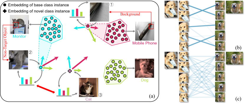
Figure 1: (a) Hard labels could provide false supervision since random cropping may alter the semantics. Describing patches by analogy, soft labels can avoid this and utilize the class-level diversity provided by random cropping. The matching flows between two sets of similar local patches using (b) EMD and (c) our Adaptive Metric.

Feature extractor is insufficiently pre-trained with hard labels only. Usually, the encoder for extracting local features will be pre-trained with a proxy task classifying all base classes, where random cropping is often inherited as a simple and effective augmentation [6, 3, 4, 7]. However, it may alter the semantics (Fig. 1 (a) \raisebox{-.9pt} {1}⃝\raisebox{-.9pt} {2}⃝), making ground-truth hard labels insufficient for pretraining encoders capable of extracting high-quality local features. The reasons are, firstly, they may provide false supervision that correlates the background or non-target objects to a base class. This is acceptable for normal intra-class classification tasks as it serves as a shortcut knowledge (e.g., dolphins are usually in the water) which improves the performance [8]. But in the few-shot setting, these priors do not hold for novel classes, which introduces bias. Secondly, they cannot utilize the class-level diversity provided by random cropping to prevent the network from overfitting to base classes. Because hard labels strictly assume that the input belongs to one of the base classes, which cannot describe patches with semantics beyond all base classes.

Indicating the probability of the input belonging to each base class, soft labels are capable of describing cropped patches by analogy (e.g., a cat is something more like a dog and less like a monitor). Therefore, they can be used to supervise the learning of these cropped patches for regularization while avoiding false supervision. Moreover, soft labels connect non-target objects with potential novel classes through similar distributions (Fig. 1 (a) \raisebox{-.9pt} {2}⃝\raisebox{-.9pt} {3}⃝), making the learning of these patches a pre-search for suitable positions to embed novel class samples, which warms up the encoder for possible test scenarios in advance.

Metric necessitates adaptability for various set compositions. Given two sets to be measured, a local relation exists for each element in their Cartesian product. The rational utilization of these local relations is essential for an effective measure. Recently, embedding randomly cropped patches stands out in constructing local feature sets [4] since it handles the uncertainty of novel classes with randomness. However, random cropping unavoidably results in various set compositions, i.e., the local features in a set may be highly similar or different to varying degrees. Different compositions need different local relation utilization, requiring the metric to be able to handle them adaptively. For example, similar features of the same set yield similar local relations which should be utilized equivalently, while dissimilar features yield disparate local relations which should be utilized differently. As a classic representative of optimal transport (OT) distances, Earth Mover’s Distance (EMD) is a well-studied set metric and applies to measuring local feature sets [1]. However, it lacks the adaptability for various set compositions. Specifically, the optimum transport matrix is usually solved on a vertex of the transport polytope, resulting in a sparse matching flow regardless of the set composition. When the set elements are highly similar, only a few local relations among several equally important ones contribute to the matching process (Fig. 1 (b)), affecting the fidelity of the similarity measure.

Introducing an entropic regularization, the Sinkhorn Distance [10] encourages smoother transport matrices, allowing “one-to-many” matching (Fig. 1 (c)) that better utilizes similar local relations. Therefore, formulating the metric as an entropy-regularized OT problem can endow the algorithm with the ability to handle similar local relations. Moreover, adaptability can be introduced into the metric by conditioning the regularization strength on set compositions.

In this paper, we propose a novel method, namely FCAM, for few-shot classification to unleash the power of local representations in improving novel-class generalization. To obtain better local features, we propose Feature Calibration to pre-train few-shot encoders. It supervises the learning of cropped patches with soft labels produced by a momentum-updated teacher, utilizing the class-level diversity of them while avoiding false supervision. In addition, by decomposing the classical KL-Divergence commonly used for soft label supervision, we find its inherent weighting scheme unsuitable for learning few-shot encoders as it implicitly assumes that the input must belong to a certain base class. Therefore, we propose UniCon KL-Divergence (UKD) with a more suitable weighting scheme for the soft label supervision. To measure local feature sets with various compositions, we propose Adaptive Metric that formulates the set measure problem as a regularized OT problem, where a Modulate Module is designed to adjust the regularization strength adaptively. The proposed method achieves new state-of-the-art performance on three popular benchmarks. Moreover, it exceeds state-of-the-art transductive and cross-modal methods in the fine-grained scenario. Our contributions are as follows:

• We propose a novel pretraining paradigm for few-shot encoders that uses soft labels to utilize the class-level diversity provided by random cropping while avoiding improper supervision.

• We propose a UniCon KL-Divergence for the soft label supervision to correct an assumption of conventional KL-Divergence that does not hold true for the few-shot setting.

• We propose a novel metric capable of handling various compositions of local feature sets adaptively for local-representation-based FSC.

2 Related Work

Metric-based few-shot classification. The literature exhibits significant diversity in the area of FSC [11, 12, 13, 3, 4, 14, 15, 16], among which metric-based methods [11, 12, 13, 3, 4] are very elegant and promising. The main idea is to meta-learn a representation expected to be generalizable across categories with a predefined [11, 12, 3, 1, 4] or also meta-learned [13] metric as the classifier. For example, Snell et al. [12] average the embeddings of congener support samples as the class prototype and leverages the Euclidean distance for classification. Sung et al. [13] replace the metric with a learnable module to introduce nonlinearity. To avoid congener image-level embeddings from being pushed far apart by the significant intra-class variations, recent approaches resort to local representations. Generally, an instance is represented by a local feature set whose elements can be implemented as local feature vectors [17, 1, 3, 4] or embeddings of patches cropped grid-like [3, 4] or randomly [4]. Then, support-query pairs are measured by a metric capable of measuring two sets, e.g., accumulated cosine similarities between nearest neighbors [17], bidirectional random walk [3] or EMD [1, 4].

Self-distillation. First proposed for model compression [18, 19, 20], knowledge distillation aims at transferring “knowledge”, such as logits [20] or intermediate features [21, 22, 23], from a high-capability teacher model to a lightweight student network. As a special case when the teacher and student architectures are identical, self-distillation has been consistently observed to achieve higher accuracy [24]. Zhang et al. [25] relate self-distillation with label smoothing, a commonly-used regularization technique to prevent models from being over-confident. Generating soft labels with a momentum-updated teacher, our Feature Calibration is closely related to self-distillation and exhibits a similar regularization effect for improving class-level generalization.

Optimal transport distances. The distances based on the well-studied OT problem are very powerful for probability measures. EMD was first proposed for image retrieval [26] and exhibited excellent performance. Cuturi [10] proposes the Sinkhorn Distance by regularizing the OT problem with an entropic term, which greatly improves the computing efficiency and defines a distance with a natural prior on the transport matrix: everything should be homogeneous in the absence of a cost. It provides an essential prior that EMD lacks for measuring sets consisting of highly similar nodes.

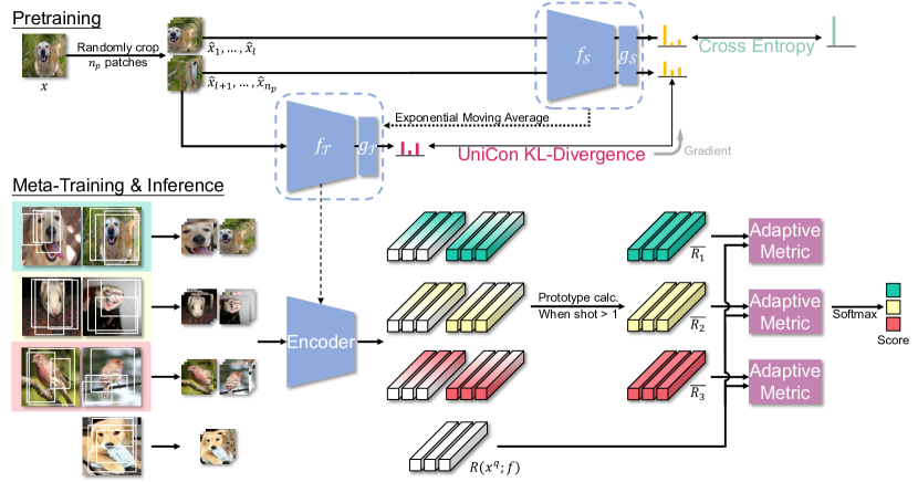
Figure 2: Overview of our framework ($3$-way $2$-shot as an example).

3 Training Paradigm

Given a labeled dataset $D_{base}=\{(x_{i}^{b},y_{i}^{b})\}_{i=1}^{N_{base}}$ composed of $n_{c}$ base classes, few-shot classification aims to construct a classifier for future tasks consisting of novel classes. Contemporary metric-based methods [6, 3, 4, 7] often adopt a “pretraining + meta-training” paradigm. In the pretraining stage, a classification network $\phi=f\circ g$ consisting of an encoder $f$ and a linear layer $g$ is trained to distinguish all base classes, i.e., $\phi(x_{i}^{b})\in\mathbb{R}^{n_{c}}$. In the meta-training stage, the encoder is fine-tuned across a large number of $N$-way $K$-shot tasks constructed from $D_{base}$ to simulate the test scenario. In a task containing $N$ classes ($N<n_{c}$), $K$ samples from each class are sampled to construct a support set $D_{spt}=\{(x_{i}^{s},y_{i}^{s})\}_{i=1}^{NK}$, according to which we need to predict labels for a query set $D_{qry}=\{(x_{i}^{q},y_{i}^{q})\}_{i=1}^{NQ}$ that contains samples from the same $N$ classes with $Q$ samples per class. Specifically, for a query sample $x_{i}^{q}$ whose ground-truth label $y_{i}^{q}=c$ ($c\in\{1,\ldots,N\}$), the pre-trained encoder $f$ is fine-tuned to maximize:

$$p(y_{i}^{q}=c\mid x_{i}^{q})=\frac{\exp{(S(R(x_{i}^{q};f),\overline{R_{c}}))}}{\sum\nolimits_{j=1}^{N}\exp{(S(R(x_{i}^{q};f),\overline{R_{j}}))}},$$ (1)

where $S(\cdot,\cdot)$ is a metric measuring the similarity between $x_{i}^{q}$’s representation $R(x_{i}^{q};f)$ and class $j$’s prototype representation $\overline{R_{j}}$.

As illustrated in Fig. 2, we integrate our method into this paradigm and focus on local representations constructed by the random cropping operation $\xi(\cdot)$, where $R(x_{i}^{q};f)$ and $\overline{R_{j}}$ are defined as:

$$\begin{split}R(x_{i}^{q};f)\coloneqq\{\mathbf{u}_{m}|m=1,2,\ldots,n\},\quad\overline{R_{j}}\coloneqq\{\mathbf{v}_{m}|m=1,2,\ldots,n\},\\ \text{where}~{}\mathbf{u}_{m}=f(\xi(x_{i}^{q})),\quad\mathbf{v}_{m}=\frac{1}{K}\sum\nolimits_{i=1}^{NK}f(\xi(x_{i}^{s}))\cdot[y_{i}^{s}=j],\end{split}$$ (2)

where $[y_{i}^{s}=j]$ is an indicator function that equals $1$ when $y_{i}^{s}=j$ and $0$ otherwise.

4 Feature Calibration

4.1 Feature Calibration with Soft Labels

Different from existing methods using only ground-truth hard labels, we propose a novel paradigm that takes soft labels into account as well for pretraining few-shot encoders. It calibrates the extracted features by avoiding false supervision while fully exploiting the class-level diversity of patches. As shown in Fig. 2, the pretraining stage involves two structurally identical networks, i.e., a student network $\phi_{\mathcal{S}}=f_{\mathcal{S}}\circ g_{\mathcal{S}}$ and a teacher network $\phi_{\mathcal{T}}=f_{\mathcal{T}}\circ g_{\mathcal{T}}$, with $f_{\mathcal{S}}$ and $f_{\mathcal{T}}$ being their respective encoders, and $g_{\mathcal{S}}$ and $g_{\mathcal{T}}$ being their respective last linear layers. Given a sample $x$ in $D_{base}$, a set of patches $\{\hat{x}_{i}|i=1,2,...,n_{p}\}$ can be obtained by random cropping (with resize and flip). We reserve the first $l$ ($0<l<n_{p}$) elements $\{\hat{x}_{1},\ldots,\hat{x}_{l}\}$ for normal hard label supervision using the cross-entropy loss:

$$\mathcal{L}_{CE}=-\mathbf{y}^{\top}\log{(\sigma(\frac{1}{l}\sum_{i=1}^{l}\phi_{\mathcal{S}}(\hat{x}_{i})))},$$ (3)

where $\sigma$ denotes the softmax function and $\mathbf{y}$ is the label of $x$ which is a one-hot vector. The remaining $n_{p}-l$ patches $\{\hat{x}_{l+1},\ldots,\hat{x}_{n_{p}}\}$ are used for soft label supervision, where we construct a momentum updated [27] teacher network $\phi_{\mathcal{T}}$ to generate soft labels. Specifically, denoting the parameters of $\phi_{\mathcal{T}}$ as $\theta_{\mathcal{T}}$ and those of $\phi_{\mathcal{S}}$ as $\theta_{\mathcal{S}}$, for the $i$-th iteration, $\theta_{\mathcal{T}}$ is updated by:

$$\theta_{\mathcal{T}}^{i}\leftarrow m\theta_{\mathcal{T}}^{i-1}+(1-m)\theta_{\mathcal{S}}^{i},$$ (4)

where $m\in[0,1)$ is a momentum coefficient. As an exponential moving average of the student, the teacher evolves more smoothly, which ensures the stability of the generated soft labels [28, 29]. To align the output of $\phi_{\mathcal{S}}$ to that of $\phi_{\mathcal{T}}$, we propose a UniCon KL-Divergence as described below.

4.2 UniCon KL-Divergence

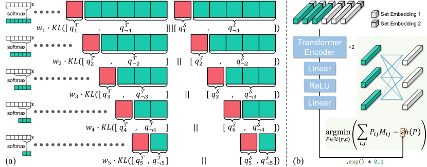
Figure 3: Illustration of (a) the continuous binary classification process corresponding to the reformulation of KL-Divergence, and (b) the proposed Adaptive Metric formulating the measure process as an OT problem. To handle various set compositions, the adjustment coefficient of an entropy regularization is tuned by a Modulate Module.

Denoting the network output for a patch as $\mathbf{z}=[z_{1},z_{2},...,z_{n_{c}}]\in\mathbb{R}^{n_{c}}$ where $z_{i}$ represents the logit of the $i$-th base class, the $n_{c}$-classification probabilities $\mathbf{p}=[p_{1},p_{2},...,p_{n_{c}}]\in\mathbb{R}^{n_{c}}$ can be defined where the probability of the patch belonging to class $i$ is given by:

$$p_{i}=\frac{\exp{(z_{i})}}{\sum\nolimits_{j=1}^{n_{c}}\exp{(z_{j})}}.$$ (5)

As a common choice to measure two probability distributions, KL-Divergence is often used for soft label supervision [20, 24, 25]. However, it is not suitable for learning few-shot encoders, which we elaborate on by decomposing it.

Decomposition of KL-Divergence. To analyze KL-Divergence in terms of the probabilities associated with each base class, the foundation of soft labels’ ability to describe patches, we consider a process shown in Fig. 3 (a). This is a process of continuous binary classification where each time we only focus on whether the input belongs to a certain class or to the remaining classes. The probabilities of the $i$-th binary classification $\mathbf{b}_{i}=[q_{i},q_{\neg i}]$ can be obtained by:

$$q_{i}=\frac{\exp{(z_{i})}}{\sum\nolimits_{j=i}^{n_{c}}\exp{(z_{j})}},\quad q_{\neg i}=\frac{\sum\nolimits_{k=i+1}^{n_{c}}\exp{(z_{k})}}{\sum\nolimits_{j=i}^{n_{c}}\exp{(z_{j})}}.$$ (6)

Note that this is a process without replacement, i.e., the calculation of $\mathbf{b}_{i}$ only involves the logits of class $i$-$n_{c}$. Converting the multivariate distribution into a series of bivariate distributions, this decomposition helps us to investigate the probabilities for distinguishing each base class, leading to the following result (the detailed proof is presented in the appendix).

Theorem 1

Marking the variables calculated using the teacher output $\mathbf{z}^{\mathcal{T}}$ and student output $\mathbf{z}^{\mathcal{S}}$ with the superscripts $\mathcal{T}$ and $\mathcal{S}$, respectively, the classical KL-Divergence for soft label supervision can be reformulated as:

$$KL(\mathbf{p}^{\mathcal{T}}||\mathbf{p}^{\mathcal{S}})=\sum\limits_{i=1}^{n_{c}-1}w_{i}\cdot KL(\mathbf{b}_{i}^{\mathcal{T}}||\mathbf{b}_{i}^{\mathcal{S}}),\quad\text{where}~{}w_{i}=\sum_{k=i}^{n_{c}}p_{k}^{\mathcal{T}}.$$ (7)

Improper weighting scheme. Theorem 1 demonstrates that, for KL-Divergence, the problem of measuring two classification probability distributions can be decomposed into measuring $\mathbf{b}_{i}$ constantly. By giving $w_{i}$, it also indicates how KL-Divergence weights the measure of $\mathbf{b}_{i}$. Since the continuous binary classification is a process without replacement, the number of remaining classes to be considered (class cardinality) differs for different $i$. Therefore, we consider a comparable form that normalizes $w_{i}$ with the class cardinality $n_{c}-i+1$:

$$\tilde{w}_{i}=\frac{1}{n_{c}-i+1}\sum_{k=i}^{n_{c}}p_{k}^{\mathcal{T}}.$$ (8)

According to $\tilde{w}_{i}$, the less similar the teacher thinks the input is to class $i$-$n_{c}$, the less important the alignment of $\mathbf{b}_{i}$. This weighting scheme is consistent with the prior of normal intra-class classification tasks, i.e., the input must belong to a certain base class. In this case, it is reasonable to stress the measure of $\mathbf{b}_{i}$ if the teacher thinks the input belongs to class $i$-$n_{c}$ or downplay it if otherwise. However, in the context of few-shot classification, the input does not belong to any base class, and the measure of different $\mathbf{b}_{i}$ should be equally important as each base class prototype is equal in serving as the manifold base to represent image features [30].

Smoother weighting scheme for uniform base class contributions. Noticing that the weighting scheme can be smoothed by smoothing $\mathbf{p}^{\mathcal{T}}$, we introduce a temperature coefficient $T$ to alter the distribution of $\mathbf{p}^{\mathcal{T}}$ inspired by its use for the same purpose in various fields, e.g., contrastive learning [28] and knowledge distillation [20]. Furthermore, we discover that the difference between the weights of two different binary classifications $\tilde{w}_{\alpha}(T)$ and $\tilde{w}_{\beta}(T)$ ($\alpha\neq\beta$) vanishes with an extremely high temperature:

$$\lim_{T\to\infty}|\tilde{w}_{\alpha}(T)-\tilde{w}_{\beta}(T)|=\lim_{T\to\infty}\bigg{|}\frac{\sum\nolimits_{k_{1}=\alpha}^{n_{c}}\exp{(z_{k_{1}}^{\mathcal{T}}/T)}}{(n_{c}-\alpha+1)\sum\nolimits_{j=1}^{n_{c}}\exp{(z_{j}^{\mathcal{T}}/T)}}-\frac{\sum\nolimits_{k_{2}=\beta}^{n_{c}}\exp{(z_{k_{2}}^{\mathcal{T}}/T)}}{(n_{c}-\beta+1)\sum\nolimits_{j=1}^{n_{c}}\exp{(z_{j}^{\mathcal{T}}/T)}}\bigg{|}=0,$$ (9)

according to which we derive a weighting scheme emphasizing the uniform contribution of different base classes for learning few-shot encoders:

$$w_{i}^{\prime}\coloneqq\lim_{T\to\infty}\frac{\sum\nolimits_{k=i}^{n_{c}}\exp{(z_{k}^{\mathcal{T}}/T)}}{\sum\nolimits_{j=1}^{n_{c}}\exp{(z_{j}^{\mathcal{T}}/T)}}=\frac{n_{c}-i+1}{n_{c}}.$$ (10)

With a more rational weighting scheme, we define UniCon KL-Divergence that is used to compute the loss for soft labels $\mathcal{L}_{UKD}$:

$$UKD(\mathbf{p}^{\mathcal{T}}||\mathbf{p}^{\mathcal{S}})\coloneqq\sum\limits_{i=1}^{n_{c}-1}w_{i}^{\prime}\cdot KL(\mathbf{b}_{i}^{\mathcal{T}}||\mathbf{b}_{i}^{\mathcal{S}}),$$ (11)

$$\mathcal{L}_{UKD}=\frac{1}{n_{p}-l}\sum\limits_{i=l+1}^{n_{p}}UKD(\sigma(\phi_{T}(\hat{x}_{i}))||\sigma(\phi_{S}(\hat{x}_{i}))).$$ (12)

And with a weight $\lambda$, $\mathcal{L}_{UKD}$ is combined with $\mathcal{L}_{CE}$ to form the total loss for pretraining:

$$\mathcal{L}_{total}=\mathcal{L}_{CE}+\lambda\cdot\mathcal{L}_{UKD}.$$ (13)

5 Adaptive Metric

After pretraining, $f_{\mathcal{T}}$ will be used as the feature extractor for further meta-training as illustrated in Fig. 2, where we propose Adaptive Metric for classification.

5.1 The Sinkhorn Distance for Few-Shot Classification

Our Adaptive Metric is based on OT distances that measure two sets by considering a hypothetical process of transporting goods from nodes of one set (suppliers) to nodes of the other set (demanders). Given the weight vectors $\mathbf{r},\mathbf{c}\in\mathbb{R}_{+}^{d}$ ($\mathbf{r}^{\top}\mathbf{1}_{d}=\mathbf{c}^{\top}\mathbf{1}_{d}=1$) where each element represents the total supply (demand) goods of a node, and the cost per unit $M_{ij}$ for transporting from supplier $i$ to demander $j$, the goal is to find a transportation plan with the lowest total cost from a set of valid plans $\mathcal{U}(\mathbf{r},\mathbf{c})=\{P\in\mathbb{R}_{+}^{n\times n}|P\mathbf{1}_{n}=\mathbf{r},P^{\top}\mathbf{1}_{n}=\mathbf{c}\}$.

In order to endow the algorithm with the ability to properly utilize similar local relations, instead of solving $\mathop{\arg\min}\nolimits_{P\in\mathcal{U}(\mathbf{r},\mathbf{c})}\sum\nolimits_{i,j}P_{ij}M_{ij}$ directly like EMD [26], we formulate the set measure problem as optimizing an entropy-regularized [10] OT problem to encourage smoother transport matrices:

$$P^{\varepsilon}=\mathop{\arg\min}\limits_{P\in\mathcal{U}(\mathbf{r},\mathbf{c})}\Bigl{(}\sum\limits_{i,j}P_{ij}M_{ij}-\varepsilon h(P)\Bigr{)},$$ (14)

where $\varepsilon\in(0,\infty)$ serves as an adjustment coefficient of the regularization term, and $h(P)=-\sum\nolimits_{i,j}P_{ij}\log{P_{ij}}$ is the information entropy of $P$, which reflects the smoothness of $P$, the higher the entropy, the smoother the solved matrix.

Given two local feature sets to be measured, i.e., $R(x_{i}^{q};f)$ and $\overline{R_{j}}$, we define the weight of each feature with its cosine similarity to the mean of the other set, along with a softmax function to convert it to a probability distribution:

$$r_{i}=\frac{\exp{(\hat{r}_{i})}}{\sum_{j=1}^{n}\exp{(\hat{r}_{j})}},\quad\text{where}~{}\hat{r}_{i}\coloneqq\frac{\mathbf{u}_{i}^{\top}\cdot\frac{1}{n}\sum_{j=1}^{n}\mathbf{v}_{j}}{\|\mathbf{u}_{i}\|\cdot\|\frac{1}{n}\sum_{j=1}^{n}\mathbf{v}_{j}\|},$$ (15)

$$c_{i}=\frac{\exp{(\hat{c}_{i})}}{\sum_{j=1}^{n}\exp{(\hat{c}_{j})}},\quad\text{where}~{}\hat{c}_{i}\coloneqq\frac{\mathbf{v}_{i}^{\top}\cdot\frac{1}{n}\sum_{j=1}^{n}\mathbf{u}_{j}}{\|\mathbf{v}_{i}\|\cdot\|\frac{1}{n}\sum_{j=1}^{n}\mathbf{u}_{j}\|}.$$ (16)

This stems from the intuition that local features more similar to the other set are more likely to be related to the concurrent foreground objects and, hence should be assigned greater weight. Then, with the cost to transport a unit from node $\mathbf{u}_{i}$ to $\mathbf{v}_{j}$ defined by their cosine similarity:

$$M_{ij}\coloneqq 1-\frac{\mathbf{u}_{i}^{\top}\mathbf{v}_{j}}{\|\mathbf{u}_{i}\|\|\mathbf{v}_{j}\|},$$ (17)

we solve the optimization problem of Eq. 14 in parallel by the Sinkhorn-Knopp algorithm [31]. Eventually, with the solved $P^{\varepsilon}$, we define Adaptive Metric to compute the classification score that is used for cross entropy calculation or inference:

$$S(R(x_{i}^{q};f_{\mathcal{T}}),\overline{R_{j}})\coloneqq\sum\limits_{i=1}^{n}\sum\limits_{j=1}^{n}(1-M_{ij})P_{ij}^{\varepsilon}.$$ (18)

5.2 Modulate Module

Furthermore, to control the smoothness of the transport matrix adaptively according to specific local feature sets, we design a Modulate Module to predict $\varepsilon$ in Eq. 14 instead of treating it as a pre-fixed hyperparameter. By giving higher $\varepsilon$, $P^{\varepsilon}$ will be smoother, and as $\varepsilon$ goes to zero, it will be sparser, with the solution close to EMD. Intuitively, the smoothness of the transport matrix should be conditioned on the relationship of the local features (similar features come with similar local patches where a smooth transport matrix is expected). Therefore, we take the extracted local features as input and construct a predictor based on the Transformer encoder [32], considering that its inductive bias suits the task of modeling the relationship between local features very well. As shown in Fig. 3 (b), the input embeddings are constructed by concatenating the local feature with a $16$ dimensional learnable set embedding indicating which set the local feature is from, i.e., $R(x_{i}^{q};f_{\mathcal{T}})$ or $\overline{R_{j}}$. Followed by an exponential function, the output serves as a scaling factor to adjust $\varepsilon$ from the default value of $0.1$.

The overall training process of our method is described in Algorithm 1.

Algorithm 1 Training process of FCAM.

1:Pretraining

2:Warm up $\phi_{\mathcal{S}}$ with $\mathcal{L}_{CE}$;

3:$\theta_{\mathcal{T}}\leftarrow\theta_{\mathcal{S}}$;

4:while epochs do

5:     while steps do

6:         Randomly crop $n_{p}$ patches $\{\hat{x}_{1},\ldots,\hat{x}_{n_{p}}\}$ for each image $x$ in the minibatch;

7:         Calculate $\mathcal{L}_{CE}$ with $\{\hat{x}_{1},\ldots,\hat{x}_{l}\}$;

8:         Calculate $\mathcal{L}_{UKD}$ with $\{\hat{x}_{l+1},\ldots,\hat{x}_{n_{p}}\}$;

9:         $\mathcal{L}_{total}=\mathcal{L}_{CE}+\lambda\cdot\mathcal{L}_{UKD}$;

10:         Update $\theta_{\mathcal{S}}$ with $\nabla_{\theta_{\mathcal{S}}}\mathcal{L}_{total}$;

11:         Update $\theta_{\mathcal{T}}$, i.e., $\theta_{\mathcal{T}}^{i}\leftarrow m\theta_{\mathcal{T}}^{i-1}+(1-m)\theta_{\mathcal{S}}^{i}$;

12:     end while

13:end while

1:Meta-Training

2:while not converged do

3:     Construct a task, i.e., sample $D_{spt}$, $D_{qry}$ from $D_{base}$;

4:     Calculate $\overline{R_{j}}$ for $j$ in $N$;

5:     for $x_{i}^{q}$ in $D_{qry}$ do

6:         Calculate $R(x_{i}^{q};f_{\mathcal{T}})$;

7:         Predict $\varepsilon$ and calculate $S(R(x_{i}^{q};f_{\mathcal{T}}),\overline{R_{j}})$ for $j$ in $N$;

8:     end for

9:     Calculate cross entropy loss;

10:     Optimize $f_{\mathcal{T}}$;

11:end while

6 Experiments

Datasets. The experiments are conducted on three popular benchmarks: (1) miniImageNet [11] is a subset of ImageNet [33] that contains 100 classes with 600 images per class. The 100 classes are divided into 64/16/20 for train/val/test respectively; (2) tieredImageNet [34] is also a subset of ImageNet [33] that includes 608 classes from 34 super-classes. The super-classes are split into 20/6/8 for train/val/test respectively; (3) CUB-200-2011 [35] contains 200 bird categories with 11,788 images, which represents a fine-grained scenario. Following the splits in [36], the 200 classes are divided into 100/50/50 for train/val/test respectively.

Backbone. For the backbone, we employ ResNet12 as many previous works. With the dimension of the embedded features and the set embeddings being 640 and 16, respectively, we set $d_{model}=656$, $d_{feedforward}=1280$ and $n_{head}=16$ for the $2$-layer Transformer encoder in our Modulate Module.

Training details. In the pretraining stage, we set $n_{p}=4$, $l=1$ and $m=0.999$. $\mathcal{L}_{UKD}$ will not be used during early epochs to ensure the teacher has well-converged before being used to generate soft labels. In the meta-training stage, each epoch involves $50$ iterations with a batch size of $4$. We set $n=25$, and the patches are resized to $84\times 84$ before being embedded. The Modulate Module is first trained for $100$ epochs with the encoder’s parameters fixed, in which the learning rate starts from $1e$-$3$ and decays by $0.1$ at epoch $60$ and $90$. Then, all the parameters will be optimized jointly for another $100$ epochs.

6.1 Comparison with State-of-the-art Methods

For general few-shot classification, we compare our method with the state-of-the-art methods in Table 1. Our method outperforms the state-of-the-art methods on all the settings and even achieves higher performance than methods with bigger backbones, achieving new state-of-the-art performance. For fine-grained few-shot classification, we compare our method with the state-of-the-art methods in Table 4. Benefit from higher quality local features, the discriminative regions can be depicted more accurately, resulting in significant improvement against other methods, i.e., $\bf{4.41\%}$ and $\bf{2.85\%}$ for $1$-shot and $5$-shot respectively against previous state-of-the-art method [3]. In particular, our method even outperforms state-of-the-art transductive [37, 38] and cross-modal [39, 38] methods, shedding some light on how much the poor local representations can degrade the performance in the fine-grained scenario.

6.2 Ablation Study

To begin with, a coarse-scale ablation is presented in Table 4. The baseline follows the traditional pretraining paradigm that uses only $\mathcal{L}_{CE}$ for supervision and employs EMD as the metric. With both Feature Calibration and Adaptive Metric outperforming the baseline and achieving optimal results when used together, their respective effectiveness can be validated. Furthermore, we conduct a more detailed analysis below.

Table 1: Comparison to the state-of-the-art methods on miniImageNet and tieredImageNet, ordered chronologically. Average $5$-way $1$-shot and $5$-way $5$-shot accuracy ($\%$) with $95\%$ confidence intervals.

Method	Backbone	miniImageNet		tieredImageNet
		$1$-shot	$5$-shot	$1$-shot	$5$-shot
MatchNet$\dagger$  [11]	ResNet12	$63.08\pm 0.80$	$75.99\pm 0.60$	$68.50\pm 0.92$	$80.60\pm 0.71$
ProtoNet$\dagger$  [12]	ResNet12	$60.37\pm 0.83$	$78.02\pm 0.57$	$65.65\pm 0.92$	$83.40\pm 0.65$
TADAM [40]	ResNet12	$58.50\pm 0.30$	$76.70\pm 0.30$	-	-
FEAT [36]	ResNet12	$66.78\pm 0.20$	$82.05\pm 0.14$	$70.80\pm 0.23$	$84.79\pm 0.16$
DeepEMD [1]	ResNet12	$65.91\pm 0.82$	$82.41\pm 0.56$	$71.16\pm 0.87$	$86.03\pm 0.58$
Meta-Baseline [6]	ResNet12	$63.17\pm 0.23$	$79.26\pm 0.17$	$68.62\pm 0.27$	$83.74\pm 0.18$
FRN [2]	ResNet12	$66.45\pm 0.19$	$82.83\pm 0.13$	$72.06\pm 0.22$	$86.89\pm 0.14$
PAL [41]	ResNet12	$\underline{69.37\pm 0.64}$	$84.40\pm 0.44$	$72.25\pm 0.72$	$86.95\pm 0.47$
MCL [3]	ResNet12	$69.31\pm 0.20$	$\underline{85.11\pm 0.20}$	$73.62\pm 0.20$	$86.29\pm 0.20$
DeepEMD v2 [4]	ResNet12	$68.77\pm 0.29$	$84.13\pm 0.53$	$\underline{74.29\pm 0.32}$	$\underline{87.08\pm 0.60}$
FADS [42]	ResNet12	$66.73\pm 0.88$	$83.51\pm 0.51$	$74.12\pm 0.74$	$86.56\pm 0.46$
Centroid Alignment$\ddagger$  [43]	WRN-28-10	$65.92\pm 0.60$	$82.85\pm 0.55$	$74.40\pm 0.68$	$86.61\pm 0.59$
Oblique Manifold$\ddagger$  [44]	ResNet18	$63.98\pm 0.29$	$82.47\pm 0.44$	$70.50\pm 0.31$	$86.71\pm 0.49$
FewTURE$\ddagger$  [45]	ViT-Small	$68.02\pm 0.88$	$84.51\pm 0.53$	$72.96\pm 0.92$	$86.43\pm 0.67$
FCAM (ours)	ResNet12	$\bf{70.47\pm 0.28}$	$\bf{85.71\pm 0.52}$	$\bf{75.02\pm 0.31}$	$\bf{88.41\pm 0.59}$

• results are reported in [4].

• methods with bigger backbones.

• The second best results are underlined.

Table 2: Comparison to the state-of-the-art methods on CUB-200-2011, ordered chronologically. Average $5$-way $1$-shot and $5$-way $5$-shot accuracy ($\%$) with $95\%$ confidence intervals.

Method	Backbone	CUB-200-2011
		$1$-shot	$5$-shot
MatchNet$\dagger$  [11]	ResNet12	$71.87\pm 0.85$	$85.08\pm 0.57$
ProtoNet$\dagger$  [12]	ResNet12	$66.09\pm 0.92$	$82.50\pm 0.58$
DeepEMD [1]	ResNet12	$75.65\pm 0.83$	$88.69\pm 0.50$
FRN$\sharp$  [2]	ResNet12	$78.86\pm 0.28$	$\underline{90.48\pm 0.16}$
MCL$\sharp$  [3]	ResNet12	$\underline{79.39\pm 0.29}$	$\underline{90.48\pm 0.49}$
DeepEMD v2 [4]	ResNet12	$79.27\pm 0.29$	$89.80\pm 0.51$
Centroid Alignment$\ddagger$  [43]	ResNet18	$74.22\pm 1.09$	$88.65\pm 0.55$
Oblique Manifold$\ddagger$  [44]	ResNet18	$78.24\pm-$	$92.15\pm-$
ECKPN$\flat$  [37]	ResNet12	$77.43\pm 0.54$	$92.21\pm 0.41$
AGAM$\natural$  [39]	ResNet12	$79.58\pm 0.25$	$87.17\pm 0.23$
ADRGN$\flat\natural$   [38]	ResNet12	$82.32\pm 0.51$	$92.97\pm 0.35$
FCAM (ours)	ResNet12	$\bf{82.89\pm 0.27}$	$\bf{93.06\pm 0.39}$

• results are reported in [4].

• methods with bigger backbones.

• reproduced using the data split we use.

• transductive methods.

• methods that use attribute information.

• The second best results are underlined.

Table 3: Ablation of Feature Calibration and Adaptive Metric. The experiments are conducted with ResNet12 on miniImageNet.

Feature	Adaptive	$1$-shot	$5$-shot
Calibration	Metric
		$67.57\pm 0.29$	$83.39\pm 0.54$
✓		$69.54\pm 0.29$	$85.28\pm 0.52$
	✓	$69.01\pm 0.28$	$84.41\pm 0.53$
✓	✓	$\bf{70.47\pm 0.28}$	$\bf{85.71\pm 0.52}$

Table 4: Comparison of using classical and UniCon KL-Divergence for calibration (top), and the results of whether using Modulate Module to adjust $\varepsilon$ (bottom).

Setting	$1$-shot	$5$-shot
Classical KL-Divergence	$69.94\pm 0.28$	$84.79\pm 0.53$
UniCon KL-Divergence	$\bf{70.47\pm 0.28}$	$\bf{85.71\pm 0.52}$
w/o Modulate Module	$69.69\pm 0.28$	$85.23\pm 0.52$
w/ Modulate Module	$\bf{70.47\pm 0.28}$	$\bf{85.71\pm 0.52}$

Feature Calibration improves novel-class generalization. To demonstrate that Feature Calibration improves novel-class generalization, we visualize the $1$-shot test accuracy change during feature calibration in Fig. 5.

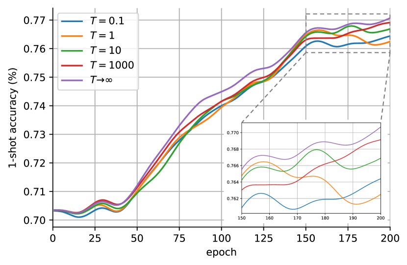
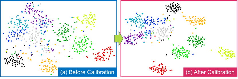
Figure 4: Gaussian smoothed $1$-shot test accuracy curves on CUB-200-2011 during feature calibration, with different temperatures to adjust the weighting scheme of the classical KL-Divergence. The results of the same $1000$ tasks are averaged for each data point.

Figure 5: Visualization [46] of novel class samples embedded by encoders trained (a) without and (b) with Feature Calibration.

We first pre-train the network to its highest validation accuracy with only $\mathcal{L}_{CE}$ to ensure the quality of the teacher and exclude the influence of hard label supervision on accuracy improvement during calibration. We observe a continuous improvement in test accuracy during calibration. In the case of our method ($T\to\infty$), the $1$-shot accuracy is boosted from $70.20\%$ to $77.41\%$, demonstrating the effectiveness of Feature Calibration in improving novel-class generalization and suggesting how severe the power of local representations is limited. In addition, the feature distributions visualized in Fig. 5 also illustrate that Feature Calibration results in better clusters for novel classes.

UniCon KL-Divergence is more suitable for Feature Calibration. We compare different temperature settings in Fig. 5. It can be seen that the temperature, i.e., the weighting scheme, affects the process of Feature Calibration. A general trend that better test accuracy comes with higher temperature can be observed, and the setting corresponding to our UniCon KL-Divergence, i.e., $T\to\infty$, constantly outperforms other settings. Furthermore, UniCon KL-Divergence yields better final performance than classical KL-Divergence as shown in Table 4. Both the above experiments demonstrate the importance of a smoother weighting scheme in Feature Calibration.

Entropic term handles sets consisting of similar nodes. For sets consisting of similar local features, the transport matrix solved by EMD (Fig. 6 (a)) is very sparse, ignoring a lot of similar local relations. In contrast, Adaptive Metric (Fig. 6 (b)) is able to generate a smoother transport matrix due to the entropic regularization, which enables a comprehensive utilization of similar local relations and reduces the dependency on a few of them by allowing “one-to-many” matching.

Modulate Module brings adaptability. For sets consisting of similar local features, Modulate Module predicts a relatively larger $\varepsilon$, resulting in a smoother transport matrix (Fig. 6 (b)). For sets consisting of dissimilar local features, a relatively smaller $\varepsilon$ is produced, making the transport matrix moderately sparse (Fig. 6 (c)). Quantitative results of whether using Modulate Module to adjust $\varepsilon$ is also presented in Table 4. Compared to a fixed default value, it introduces adaptability into the measure process, helping achieve better performance.

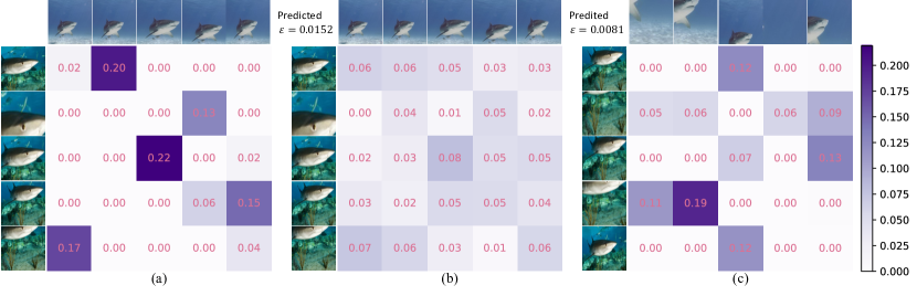
Figure 6: Visualization of solved transport matrices. Results of (a) EMD and (b) Adaptive Metric for sets consisting of similar local features, and the result of (c) Adaptive Metric for sets consisting of dissimilar local features.

6.3 Cross-Domain Experiments

For the cross-domain setting which poses a greater challenge for novel-class generalization, we perform an experiment where models are trained on miniImagenet and evaluated on CUB-200-2011. This setting allows us to better evaluate the model’s ability to handle novel classes with significant domain differences from the base classes, due to the large domain gap. As shown in Table 6, our method outperforms the previous state of the art, demonstrating its superiority in improving novel-class generalization.

Table 5: Cross-domain experiments following the setting of [47] (miniImageNet$\rightarrow$CUB). Average $5$-way $1$-shot and $5$-way $5$-shot accuracy ($\%$) with $95\%$ confidence intervals.

Method	$1$-shot	$5$-shot
ProtoNet$\dagger$  [12]	$50.01\pm 0.82$	$72.02\pm 0.67$
MatchNet$\dagger$  [11]	$51.65\pm 0.84$	$69.14\pm 0.72$
cosine classifier [47]	$44.17\pm 0.78$	$69.01\pm 0.74$
linear classifier [47]	$50.37\pm 0.79$	$73.30\pm 0.69$
KNN [17]	$50.84\pm 0.81$	$71.25\pm 0.69$
DeepEMD v2 [4]	$\underline{54.24\pm 0.86}$	$\underline{78.86\pm 0.65}$
FCAM (ours)	$\bf{58.20\pm 0.30}$	$\bf{80.92\pm 0.65}$

• results are reported in [4].

• The second best results are underlined.

Table 6: Results of global-representation-based FSC methods on miniImageNet, w/o and w/ Feature Calibration (FC). Average $5$-way $1$-shot and $5$-way $5$-shot accuracy ($\%$) with $95\%$ confidence intervals.

Method	Setting	$1$-shot	$5$-shot
cosine classifier [47]	w/o FC	$61.31\pm 0.20$	$77.73\pm 0.21$
	w/ FC	$\bf{64.92\pm 0.20}$	$\bf{80.51\pm 0.21}$
linear classifier [47]	w/o FC	$55.74\pm 0.20$	$78.89\pm 0.21$
	w/ FC	$\bf{59.35\pm 0.20}$	$\bf{81.46\pm 0.20}$
Classifier-Baseline [6]	w/o FC	$60.67\pm 0.21$	$78.53\pm 0.21$
	w/ FC	$\bf{64.33\pm 0.21}$	$\bf{81.01\pm 0.21}$
Meta-Baseline [6]	w/o FC	$63.62\pm 0.21$	$80.25\pm 0.20$
	w/ FC	$\bf{64.90\pm 0.21}$	$\bf{81.04\pm 0.21}$

6.4 Feature Calibration for Global-Representation-based FSC

Although Feature Calibration is proposed for improving local representations, it also benefits methods based on global representations as demonstrated in Table 6. Feature Calibration boosts the performance of these methods significantly due to its ability to leverage the class-level diversity provided by random cropping.

7 Conclusion

In this paper, we presented a novel FCAM method for few-shot classification to unleash the power of local representations in improving novel-class generalization. It improves the few-shot encoder by calibrating it towards the test scenario and handles various set compositions of local feature sets adaptively. Our method achieves new state-of-the-art performance on multiple datasets. To further enhance FCAM, we will seek better strategies for constructing local feature sets because a notable limitation of FCAM is the reliance of the performance on the patch number, which brings considerable computational cost.

Appendix

The appendix is organized as follows:

• Sec. A presents the proof of Theorem 1;

• Sec. B describes our experimental setup in detail;

• Sec. C shows some additional experimental results, including some analysis on computational time (Sec. C.1) and more visualized transport matrices (Sec. C.2) as a supplement to Fig. 6.

Appendix A Proof of Theorem 1

According to the definition of $q_{i}$ and $w_{i}$, $q_{i}=\frac{p_{i}}{\sum\nolimits_{k=i}^{n_{c}}p_{k}}$, hence $p_{i}^{\mathcal{T}}=w_{i}\cdot q_{i}^{\mathcal{T}}$. Therefore, we have:

$$KL(\mathbf{p}^{\mathcal{T}}||\mathbf{p}^{\mathcal{S}})=\sum_{i=1}^{n_{c}}p_{i}^{\mathcal{T}}\log\frac{p_{i}^{\mathcal{T}}}{p_{i}^{\mathcal{S}}}=\sum_{i=1}^{n_{c}}p_{i}^{\mathcal{T}}\log\frac{q_{i}^{\mathcal{T}}}{q_{i}^{\mathcal{S}}}+\sum_{i=1}^{n_{c}}p_{i}^{\mathcal{T}}\log\frac{\sum_{k=i}^{n_{c}}p_{k}^{\mathcal{T}}}{\sum_{k=i}^{n_{c}}p_{k}^{\mathcal{S}}},$$ (19)

$$\sum_{i=1}^{n_{c}}p_{i}^{\mathcal{T}}\log\frac{q_{i}^{\mathcal{T}}}{q_{i}^{\mathcal{S}}}=\sum_{i=1}^{n_{c}}w_{i}\cdot q_{i}^{\mathcal{T}}\log\frac{q_{i}^{\mathcal{T}}}{q_{i}^{\mathcal{S}}}.$$ (20)

And according to $q_{\neg i}=1-q_{i}=\frac{\sum\nolimits_{k=i+1}^{n_{c}}p_{k}}{\sum\nolimits_{k=i}^{n_{c}}p_{k}}$, we have $\sum_{k=i+1}^{n_{c}}p_{k}^{\mathcal{T}}=w_{i}\cdot q_{\neg i}^{\mathcal{T}}$, and:

$$\sum_{k=i}^{n_{c}}p_{k}=q_{\neg(i-1)}\cdot\sum_{k=i-1}^{n_{c}}p_{k}=(\prod_{k=1}^{i-1}q_{\neg k})\cdot(\sum_{k=1}^{n_{c}}p_{k})=\prod_{k=1}^{i-1}q_{\neg k}.$$ (21)

From the above equation, it can be concluded that:

$$\begin{split}\sum_{i=1}^{n_{c}}p_{i}^{\mathcal{T}}\log\frac{\sum_{k=i}^{n_{c}}p_{k}^{\mathcal{T}}}{\sum_{k=i}^{n_{c}}p_{k}^{\mathcal{S}}}=&\sum_{i=1}^{n_{c}}p_{i}^{\mathcal{T}}\log{(\prod_{k=1}^{i-1}\frac{q_{\neg k}^{\mathcal{T}}}{q_{\neg k}^{\mathcal{S}}})}=\sum_{i=1}^{n_{c}}\sum_{k=1}^{i-1}p_{i}^{\mathcal{T}}\log\frac{q_{\neg k}^{\mathcal{T}}}{q_{\neg k}^{\mathcal{S}}}\\ =&\sum_{k=1}^{n_{c}-1}\sum_{i=k+1}^{n_{c}}p_{i}^{\mathcal{T}}\log\frac{q_{\neg k}^{\mathcal{T}}}{q_{\neg k}^{\mathcal{S}}}=\sum_{k=1}^{n_{c}-1}w_{k}\cdot q_{\neg k}^{\mathcal{T}}\log\frac{q_{\neg k}^{\mathcal{T}}}{q_{\neg k}^{\mathcal{S}}}.\end{split}$$ (22)

Therefore, the KL-Divergence can be reformulated as follows:

$$\begin{split}&KL(\mathbf{p}^{\mathcal{T}}||\mathbf{p}^{\mathcal{S}})=\sum_{i=1}^{n_{c}}w_{i}\cdot q_{i}^{\mathcal{T}}\log\frac{q_{i}^{\mathcal{T}}}{q_{i}^{\mathcal{S}}}+\sum_{k=1}^{n_{c}-1}w_{k}\cdot q_{\neg k}^{\mathcal{T}}\log\frac{q_{\neg k}^{\mathcal{T}}}{q_{\neg k}^{\mathcal{S}}}\\ =&\sum_{i=1}^{n_{c}-1}w_{i}\cdot(q_{i}^{\mathcal{T}}\log\frac{q_{i}^{\mathcal{T}}}{q_{i}^{\mathcal{S}}}+q_{\neg i}^{\mathcal{T}}\log\frac{q_{\neg i}^{\mathcal{T}}}{q_{\neg i}^{\mathcal{S}}})=\sum_{i=1}^{n_{c}-1}w_{i}\cdot KL(\mathbf{b}_{i}^{\mathcal{T}}||\mathbf{b}_{i}^{\mathcal{S}}).\end{split}$$ (23)

Appendix B Detailed Experimental Setup

Following the “pretraining + meta-training” paradigm, the training process of our method can be divided into two stages. For the pretraining stage, we pre-train the encoder with our proposed pretraining paradigm based on the proxy task of standard multi-classification on $D_{base}$ and select the model with the highest validation accuracy. For the meta-training stage, each epoch involves 50 iterations with a batch size of 4. We first pre-train the Modulate Module with the parameters of the encoder fixed. Then, the parameters of both the encoder and the Modulate Module are optimized jointly. Globally, we set $n_{p}=4$, $l=1$, $m=0.999$, and $n=25$. The cropped patches are resized to $84\times 84$ before being embedded. For evaluation, we randomly sample $5000$/$600$ episodes for testing and report the average accuracy with the $95\%$ confidence interval for $1$-shot/$5$-shot experiment following [4]. In the following, we describe our detailed experimental setup according to different benchmarks:

• miniImageNet. The encoder is first pre-trained for $360$ epochs where the SGD optimizer with a momentum of $0.9$ and a weight decay of $5e$-$4$ is adopted. $\mathcal{L}_{UKD}$ will not be used for the first $120$ epochs to ensure the teacher has well-converged before being used. For the latter $240$ epochs, the learning rate is set to $0.01$, and $\lambda$ is set to $0.1$. Then, in an episodic manner, the Modulate Module is pre-trained for $100$ epochs with the parameters of the encoder fixed, in which the Adam optimizer with a weight decay of $5e$-$4$ is adopted. The learning rate starts from $1e$-$3$ and decays by $0.1$ at epoch $60$ and $90$. Finally, all the parameters will be optimized jointly for another $100$ epochs where the SGD optimizer with a momentum of $0.9$ and a weight decay of $5e$-$4$ is adopted. The learning rate starts from $5e$-$4$ and decays by $0.5$ every 10 epochs.

• tieredImageNet. The encoder is first pre-trained for $240$ epochs where the SGD optimizer with a momentum of $0.9$ and a weight decay of $5e$-$4$ is adopted. $\mathcal{L}_{UKD}$ will not be used for the first $120$ epochs to ensure the teacher has well-converged before being used. For the latter $120$ epochs, the learning rate is set to $0.001$, and $\lambda$ is set to $0.05$. Then, in an episodic manner, the Modulate Module is pre-trained for $100$ epochs with the parameters of the encoder fixed, in which the Adam optimizer with a weight decay of $5e$-$4$ is adopted. The learning rate starts from $1e$-$3$ and decays by $0.1$ at epoch $60$ and $90$. Finally, all the parameters will be optimized jointly for another $100$ epochs where the SGD optimizer with a momentum of $0.9$ and a weight decay of $5e$-$4$ is adopted. The learning rate starts from $1e$-$4$ and decays by $0.5$ every 10 epochs.

• CUB-200-2011. Each image is first cropped with the provided human-annotated bounding box as many previous works [48, 3, 4]. The encoder is first pre-trained for $360$ epochs where the SGD optimizer with a momentum of $0.9$ and a weight decay of $5e$-$4$ is adopted. $\mathcal{L}_{UKD}$ will not be used for the first $120$ epochs to ensure the teacher has well-converged before being used. For the latter $240$ epochs, the learning rate is set to $0.03$, and $\lambda$ is set to $0.5$. Then, in an episodic manner, the Modulate Module is pre-trained for $100$ epochs with the parameters of the encoder fixed, in which the Adam optimizer with a weight decay of $5e$-$4$ is adopted. The learning rate starts from $1e$-$3$ and decays by $0.1$ at epoch $60$ and $90$. Finally, all the parameters will be optimized jointly for another $100$ epochs where the SGD optimizer with a momentum of $0.9$ and a weight decay of $5e$-$4$ is adopted. The learning rate starts from $1e$-$3$ and decays by $0.5$ every 10 epochs.

Appendix C Additional Experimental Results

C.1 Analysis on Computational Time

Although the Modulate Module will inevitably bring additional time overhead during inference as a parameterized module, the proposed Adaptive Metric still costs less time for measuring two feature sets compared to EMD since the solution of the OT problem is accelerated. Specifically, the introduced entropic regularization makes the OT problem a strictly convex problem [10]. Thus, it can be solved by the Sinkhorn-Knopp algorithm [31] which is known to have a linear convergence [49, 50]. We conduct an experiment on an RTX-3090 (Linux, PyTorch 3.6) using the same $10,000$ randomly sampled episodes to compare the time cost empirically. The average time spent to process an episode is reported in Table A. It can be seen that our Adaptive Metric spends way less time than EMD ($26.33\%$ faster) even in the presence of a parameterized module, demonstrating its superiority in both accuracy and speed.

We also analyzed the influence of the number of patches used to represent an image as shown in Table B. While it shows good robustness, a limitation of FCAM is also revealed. Better accuracy requires more patches, which will result in more time for embedding them and solving the optimal transport problem. To mitigate the dependence of accuracy on the number of patches and reduce the computational cost, how to actively select most relevant patches for constructing local feature sets is an important problem to be addressed in the future.

Table A: Time spent processing an episode for methods with different metrics. 9 patches are used to represent a sample.

Metric	Average time per task (ms)
EMD	378.42
Adaptive Metric (ours)	278.78

Table B: The $1$-shot accuracy and the average time spent per task when representing an image with different numbers of patches.

# of patches	miniImageNet		CUB-200-2011
	$1$-shot acc	Time/task (ms)	$1$-shot acc	Time/task (ms)
$9$	$69.42\pm 0.28$	$\bf{478.95}$	$82.34\pm 0.27$	$\bf{278.16}$
$16$	$69.93\pm 0.28$	$816.07$	$82.86\pm 0.27$	$499.14$
$25$	$\bf{70.47\pm 0.28}$	$1334.27$	$\bf{82.89\pm 0.27}$	$780.18$

C.2 Visualization of Solved Transport Matrices

For Fig. 6, we provide more results in Fig. A.

For sets consisting of similar local patches, the transport matrices solved by EMD (Fig. A (a))) tend to be very sparse, which is not a desired property because it utilizes equivalent local relations unevenly, neglecting the information provided by lots of important local relations. In contrast, Adaptive Metric (Fig. A (b))) generates smoother transport matrices. By allowing “one-to-many” matching, it enables a comprehensive utilization of all equivalent local patches and reduces the dependency on a few of them.

By making $\varepsilon$ a learnable parameter, the Modulate Module can control the smoothness of the transport matrix self-adaptively. For sets consisting of similar local patches, the Modulate Module produces a relatively larger $\varepsilon$, resulting in a smoother transport matrix (Fig. A (b))). While for sets consisting of dissimilar local patches, a relatively smaller $\varepsilon$ is predicted, making the transport matrix moderately sparse (Fig. A (c))). The Modulate Module makes it possible for our method to handle various set compositions by introducing adaptability into the measure process.

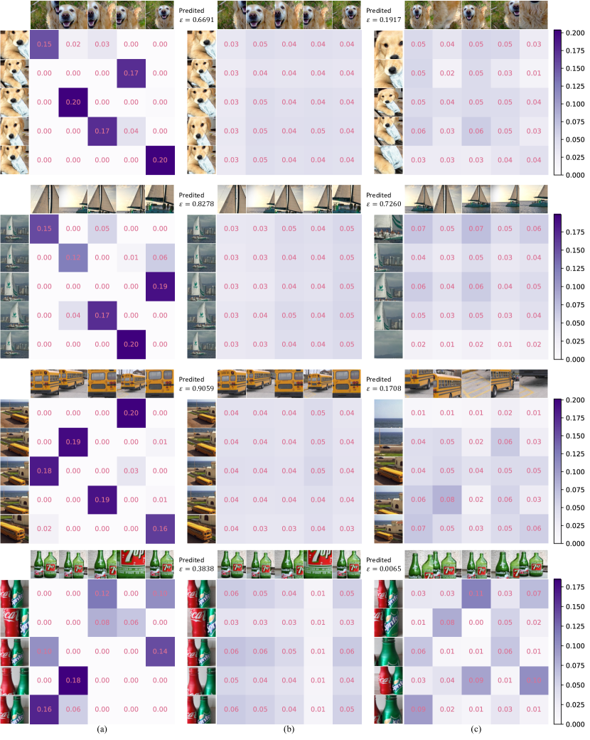
Figure A: Visualization of solved transport matrices. Results of (a) EMD and (b) Adaptive Metric for sets consisting of similar local features, and the result of (c) Adaptive Metric for sets consisting of dissimilar local features.

References

- [1] Chi Zhang, Yujun Cai, Guosheng Lin, and Chunhua Shen. Deepemd: Few-shot image classification with differentiable earth mover’s distance and structured classifiers. In Proceedings of the IEEE/CVF Conference on Computer Vision and Pattern Recognition (CVPR), June 2020.
- [2] Davis Wertheimer, Luming Tang, and Bharath Hariharan. Few-shot classification with feature map reconstruction networks. In Proceedings of the IEEE/CVF Conference on Computer Vision and Pattern Recognition (CVPR), pages 8012–8021, June 2021.
- [3] Yang Liu, Weifeng Zhang, Chao Xiang, Tu Zheng, Deng Cai, and Xiaofei He. Learning to affiliate: Mutual centralized learning for few-shot classification. In Proceedings of the IEEE/CVF Conference on Computer Vision and Pattern Recognition (CVPR), pages 14411–14420, June 2022.
- [4] Chi Zhang, Yujun Cai, Guosheng Lin, and Chunhua Shen. Deepemd: Differentiable earth mover’s distance for few-shot learning. IEEE Transactions on Pattern Analysis and Machine Intelligence, 45(5):5632–5648, 2023.
- [5] Eric Xing, Michael Jordan, Stuart J Russell, and Andrew Ng. Distance metric learning with application to clustering with side-information. In Advances in Neural Information Processing Systems, volume 15, 2002.
- [6] Yinbo Chen, Zhuang Liu, Huijuan Xu, Trevor Darrell, and Xiaolong Wang. Meta-baseline: Exploring simple meta-learning for few-shot learning. In Proceedings of the IEEE/CVF International Conference on Computer Vision (ICCV), pages 9062–9071, October 2021.
- [7] Shell Xu Hu, Da Li, Jan Stühmer, Minyoung Kim, and Timothy M. Hospedales. Pushing the limits of simple pipelines for few-shot learning: External data and fine-tuning make a difference. In Proceedings of the IEEE/CVF Conference on Computer Vision and Pattern Recognition (CVPR), pages 9068–9077, June 2022.
- [8] Kai Yuanqing Xiao, Logan Engstrom, Andrew Ilyas, and Aleksander Madry. Noise or signal: The role of image backgrounds in object recognition. In International Conference on Learning Representations, 2021.
- [9] Emmanuel J. Candès, Xiaodong Li, Yi Ma, and John Wright. Robust principal component analysis? J. ACM, 58(3), Jun 2011.
- [10] Marco Cuturi. Sinkhorn distances: Lightspeed computation of optimal transport. In Advances in Neural Information Processing Systems, volume 26, 2013.
- [11] Oriol Vinyals, Charles Blundell, Timothy Lillicrap, koray kavukcuoglu, and Daan Wierstra. Matching networks for one shot learning. In Advances in Neural Information Processing Systems, volume 29, 2016.
- [12] Jake Snell, Kevin Swersky, and Richard Zemel. Prototypical networks for few-shot learning. In Advances in Neural Information Processing Systems, volume 30, 2017.
- [13] Flood Sung, Yongxin Yang, Li Zhang, Tao Xiang, Philip H.S. Torr, and Timothy M. Hospedales. Learning to compare: Relation network for few-shot learning. In Proceedings of the IEEE Conference on Computer Vision and Pattern Recognition (CVPR), June 2018.
- [14] Chelsea Finn, Pieter Abbeel, and Sergey Levine. Model-agnostic meta-learning for fast adaptation of deep networks. In Proceedings of the 34th International Conference on Machine Learning, volume 70 of Proceedings of Machine Learning Research, pages 1126–1135, 06–11 Aug 2017.
- [15] Eli Schwartz, Leonid Karlinsky, Joseph Shtok, Sivan Harary, Mattias Marder, Abhishek Kumar, Rogerio Feris, Raja Giryes, and Alex Bronstein. Delta-encoder: an effective sample synthesis method for few-shot object recognition. In Advances in Neural Information Processing Systems, volume 31, 2018.
- [16] Huaiyu Li, Weiming Dong, Xing Mei, Chongyang Ma, Feiyue Huang, and Bao-Gang Hu. LGM-net: Learning to generate matching networks for few-shot learning. In Proceedings of the 36th International Conference on Machine Learning, volume 97 of Proceedings of Machine Learning Research, pages 3825–3834, 09–15 Jun 2019.
- [17] Wenbin Li, Lei Wang, Jinglin Xu, Jing Huo, Yang Gao, and Jiebo Luo. Revisiting local descriptor based image-to-class measure for few-shot learning. In Proceedings of the IEEE/CVF Conference on Computer Vision and Pattern Recognition (CVPR), June 2019.
- [18] Cristian Buciluundefined, Rich Caruana, and Alexandru Niculescu-Mizil. Model compression. In Proceedings of the 12th ACM SIGKDD International Conference on Knowledge Discovery and Data Mining, KDD ’06, page 535–541, 2006.
- [19] Jimmy Ba and Rich Caruana. Do deep nets really need to be deep? In Advances in Neural Information Processing Systems, volume 27, 2014.
- [20] Geoffrey Hinton, Oriol Vinyals, and Jeff Dean. Distilling the Knowledge in a Neural Network. arXiv e-prints, page arXiv:1503.02531, March 2015.
- [21] Junho Yim, Donggyu Joo, Jihoon Bae, and Junmo Kim. A gift from knowledge distillation: Fast optimization, network minimization and transfer learning. In Proceedings of the IEEE Conference on Computer Vision and Pattern Recognition (CVPR), July 2017.
- [22] Jangho Kim, Seonguk Park, and Nojun Kwak. Paraphrasing complex network: Network compression via factor transfer. In Advances in Neural Information Processing Systems, volume 31, 2018.
- [23] Byeongho Heo, Jeesoo Kim, Sangdoo Yun, Hyojin Park, Nojun Kwak, and Jin Young Choi. A comprehensive overhaul of feature distillation. In Proceedings of the IEEE/CVF International Conference on Computer Vision (ICCV), October 2019.
- [24] Tommaso Furlanello, Zachary Lipton, Michael Tschannen, Laurent Itti, and Anima Anandkumar. Born again neural networks. In Proceedings of the 35th International Conference on Machine Learning, volume 80 of Proceedings of Machine Learning Research, pages 1607–1616, 10–15 Jul 2018.
- [25] Zhilu Zhang and Mert Sabuncu. Self-distillation as instance-specific label smoothing. In Advances in Neural Information Processing Systems, volume 33, pages 2184–2195, 2020.
- [26] Y. Rubner, L. Guibas, and C. Tomasi. The earth mover”s distance, multidimensional scaling, and color-based image retrieval. Proceedings of the Arpa Image Understanding Workshop, 1997.
- [27] Antti Tarvainen and Harri Valpola. Mean teachers are better role models: Weight-averaged consistency targets improve semi-supervised deep learning results. In Advances in Neural Information Processing Systems, volume 30, 2017.
- [28] Kaiming He, Haoqi Fan, Yuxin Wu, Saining Xie, and Ross Girshick. Momentum contrast for unsupervised visual representation learning. In Proceedings of the IEEE/CVF Conference on Computer Vision and Pattern Recognition (CVPR), June 2020.
- [29] Jean-Bastien Grill, Florian Strub, Florent Altché, Corentin Tallec, Pierre Richemond, Elena Buchatskaya, Carl Doersch, Bernardo Avila Pires, Zhaohan Guo, Mohammad Gheshlaghi Azar, Bilal Piot, koray kavukcuoglu, Remi Munos, and Michal Valko. Bootstrap your own latent - a new approach to self-supervised learning. In Advances in Neural Information Processing Systems, volume 33, pages 21271–21284, 2020.
- [30] Zhongqi Yue, Hanwang Zhang, Qianru Sun, and Xian-Sheng Hua. Interventional few-shot learning. In Advances in Neural Information Processing Systems, volume 33, pages 2734–2746, 2020.
- [31] Richard Sinkhorn and Paul Knopp. Concerning nonnegative matrices and doubly stochastic matrices. Pacific Journal of Mathematics, 21(2):343–348, 1967.
- [32] Ashish Vaswani, Noam Shazeer, Niki Parmar, Jakob Uszkoreit, Llion Jones, Aidan N Gomez, Ł ukasz Kaiser, and Illia Polosukhin. Attention is all you need. In Advances in Neural Information Processing Systems, volume 30, 2017.
- [33] Olga Russakovsky, Jia Deng, Hao Su, Jonathan Krause, Sanjeev Satheesh, Sean Ma, Zhiheng Huang, Andrej Karpathy, Aditya Khosla, Michael Bernstein, et al. Imagenet large scale visual recognition challenge. International journal of computer vision, 115:211–252, 2015.
- [34] Mengye Ren, Eleni Triantafillou, Sachin Ravi, Jake Snell, Kevin Swersky, Joshua B. Tenenbaum, Hugo Larochelle, and Richard S. Zemel. Meta-learning for semi-supervised few-shot classification. In Proceedings of 6th International Conference on Learning Representations ICLR, 2018.
- [35] Catherine Wah, Steve Branson, Peter Welinder, Pietro Perona, and Serge Belongie. The caltech-ucsd birds-200-2011 dataset. 2011.
- [36] Han-Jia Ye, Hexiang Hu, De-Chuan Zhan, and Fei Sha. Few-shot learning via embedding adaptation with set-to-set functions. In Proceedings of the IEEE/CVF Conference on Computer Vision and Pattern Recognition (CVPR), June 2020.
- [37] Chaofan Chen, Xiaoshan Yang, Changsheng Xu, Xuhui Huang, and Zhe Ma. Eckpn: Explicit class knowledge propagation network for transductive few-shot learning. In Proceedings of the IEEE/CVF Conference on Computer Vision and Pattern Recognition (CVPR), pages 6596–6605, June 2021.
- [38] Chaofan Chen, Xiaoshan Yang, Ming Yan, and Changsheng Xu. Attribute-guided dynamic routing graph network for transductive few-shot learning. In Proceedings of the 30th ACM International Conference on Multimedia, MM ’22, page 6259–6268, 2022.
- [39] Siteng Huang, Min Zhang, Yachen Kang, and Donglin Wang. Attributes-guided and pure-visual attention alignment for few-shot recognition. Proceedings of the AAAI Conference on Artificial Intelligence, 35(9):7840–7847, May 2021.
- [40] Boris Oreshkin, Pau Rodríguez López, and Alexandre Lacoste. Tadam: Task dependent adaptive metric for improved few-shot learning. In Advances in Neural Information Processing Systems, volume 31, 2018.
- [41] Jiawei Ma, Hanchen Xie, Guangxing Han, Shih-Fu Chang, Aram Galstyan, and Wael Abd-Almageed. Partner-assisted learning for few-shot image classification. In Proceedings of the IEEE/CVF International Conference on Computer Vision (ICCV), pages 10573–10582, October 2021.
- [42] Shuai Shao, Yan Wang, Bin Liu, Weifeng Liu, Yanjiang Wang, and Baodi Liu. Fads: Fourier-augmentation based data-shunting for few-shot classification. IEEE Transactions on Circuits and Systems for Video Technology, pages 1–1, 2023.
- [43] Arman Afrasiyabi, Jean-François Lalonde, and Christian Gagn’e. Associative alignment for few-shot image classification. In European Conference on Computer Vision (ECCV), pages 18–35. Springer, 2020.
- [44] Guodong Qi, Huimin Yu, Zhaohui Lu, and Shuzhao Li. Transductive few-shot classification on the oblique manifold. In Proceedings of the IEEE/CVF International Conference on Computer Vision (ICCV), pages 8412–8422, October 2021.
- [45] Markus Hiller, Rongkai Ma, Mehrtash Harandi, and Tom Drummond. Rethinking generalization in few-shot classification. In Advances in Neural Information Processing Systems (NeurIPS), 2022.
- [46] Laurens van der Maaten and Geoffrey Hinton. Visualizing data using t-sne. Journal of Machine Learning Research, 9(86):2579–2605, 2008.
- [47] Wei-Yu Chen, Yen-Cheng Liu, Zsolt Kira, Yu-Chiang Wang, and Jia-Bin Huang. A closer look at few-shot classification. In International Conference on Learning Representations, 2019.
- [48] Eleni Triantafillou, Richard Zemel, and Raquel Urtasun. Few-shot learning through an information retrieval lens. In Advances in Neural Information Processing Systems, volume 30, 2017.
- [49] Joel Franklin and Jens Lorenz. On the scaling of multidimensional matrices. Linear Algebra and its Applications, 114-115:717–735, 1989.
- [50] Philip A. Knight. The sinkhorn–knopp algorithm: Convergence and applications. SIAM Journal on Matrix Analysis and Applications, 30(1):261–275, 2008.