Towards Unsupervised Speaker Diarization System for Multilingual Telephone Calls Using Pre-trained Whisper Model and
Mixture of Sparse Autoencoders

Abstract

Existing speaker diarization systems heavily rely on large amounts of manually annotated data, which is labor-intensive and challenging to collect in real-world scenarios. Additionally, the language-specific constraint in speaker diarization systems significantly hinders their applicability and scalability in multilingual settings. In this paper, we therefore propose a cluster-based speaker diarization system for multilingual telephone call applications. The proposed system supports multiple languages and does not require large-scale annotated data for the training process as leveraging the multilingual Whisper model to extract speaker embeddings and proposing a novel Mixture of Sparse Autoencoders (Mix-SAE) network architecture for unsupervised speaker clustering. Experimental results on the evaluating dataset derived from two-speaker subsets of CALLHOME and CALLFRIEND telephonic speech corpora demonstrate superior efficiency of the proposed Mix-SAE network to other autoencoder-based clustering methods. The overall performance of our proposed system also indicates the promising potential of our approach in developing unsupervised multilingual speaker diarization applications within the context of limited annotated data and enhancing the integration ability into comprehensive multi-task speech analysis systems (i.e. multiple tasks of speech-to-text, language detection, speaker diarization integrated in a low-complexity system).

Keywords:— Unsupervised speaker diarization, Whisper, Mixture of sparse autoencoders, Deep clustering, Telephone call.

I Introduction

In the realm of Internet of Sounds (IoS) development, sound-based applications have drawn significant attention from the research community and have become an integral part in the forefront of driving innovation. These applications involve advanced audio processing techniques to analyze, interpret various types of sound data (e.g. acoustic scenes [1, 2, 3], sound events [4, 5], machinery sound [6], human speech [7]), enabling the core functionality and intelligence of IoS systems [8]. Regarding sound-based applications related to human speech analysis, speaker diarization, which involves identifying and segmenting audio streams by speaker identity, stands out as an important component for a variety of applications in communication (e.g. customer support call), security (e.g. voice tracking), healthcare (e.g. patient monitoring), smart home (e.g. personal assistant), etc. This component makes IoS systems more intelligent, interactive and responsive. Typically, a cluster-based speaker diarization system consists of five sub-modules (i.e. traditional cluster-based speaker diarization is described at the top of Fig. 1). The preprocessing module first converts raw audio data into suitable format for subsequent stages. The voice activity detection (VAD) module then extracts speech segments. The detected speech segments are split into fixed-length speaker-uniform segments in the segmentation sub-module. Next, the speaker embedding extractor transforms these speaker-uniform segments into fixed-length vectors as speaker representations that capture speaker characteristics. Finally, speaker labels are assigned to all the speaker-uniform segments via a clustering algorithm. Among these modules above, speaker embedding and clustering modules present crucial components in improving the overall performance of a cluster-based speaker diarization system [9, 10].

Regarding the speaker embedding extractor, numerous approaches have been proposed and successfully explored speaker features, ranging from metric-based models (GLR [11], BIC [12], etc), parametric probabilistic models (GMM-UBM [13], i-vectors [14], etc) to neural network-based models (d-vectors [15], x-vectors [16], etc). One common aspect among all mentioned methods is the necessity for a substantial amount of annotated data, especially for neural network-based approaches. This large-scale data is utilized to train and optimize the speaker feature extractors. However, training speaker embedding extractors on one type of dataset might lead to reducing the ability of these feature extractors to produce good representation for diverse data sources in practice during the inference process, especially data from different domains or unseen data. In addition, datasets for speaker diarization mainly support one single language, due to the labor-intensive and time-consuming nature of collecting and annotating data, coupled with insufficient availability of data from diverse languages. This limitation restricts the effectiveness of speaker diarization system and its integration into multilingual speech analysis applications.

With regard to the clustering module, common clustering methods have been proposed such as Agglomerative Hierarchical Clustering (AHC) [17], k-Means [18], Mean-shift [19]. However, these clustering methods do not incorporate any representation learning technique to capture underlying patterns in the data since they directly work on the input vector space and highly depend on the distance-based metrics. Although there are a few neural network-based different deep clustering frameworks for speaker embeddings involving several representation learning techniques such as DNN [20], GAN [21], Autoencoder [22], these frameworks require pre-extracted speaker embeddings (e.g. x-vectors) that fit on certain datasets. Additionally, these proposed systems are still evaluated on one single language, mainly English.

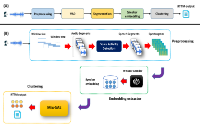
Figure 1: The high-level architectures of (A) Conventional speaker diarization system and (B) Our proposed unsupervised-based speaker diarization system

To deal with the aforementioned limitations, we aim to develop an unsupervised speaker diarization system that does not depend on the requirement of large training datasets as well as support multiple languages. To this end, at the speaker embedding module, we leverage the state-of-the-art pre-trained Whisper model for the step of speaker embedding extraction. Whisper [23] is a multilingual general-purpose model trained on massive data of diverse audio for speech recognition, language identification and speech translation. Benefiting from enhanced scalability, robustness and generalization in diverse training data of Whisper model, we are inspired to explore its potential to produce good speaker embeddings for the speaker diarization task. At the clustering module, we propose a novel unsupervised deep neural network, referred to as Mixture of Sparse Autoencoders (Mix-SAE), for clustering the extracted speaker embeddings. Our key contributions can be summarized as follows:

• We explored the potential of using general-purpose model (e.g. Whisper) as an alternative to conventional speaker embedding extractors, thus removing the need for annotated training data.

• Inspired by the work in [24], we proposed Mix-SAE network for speaker clustering that jointly improves both speaker representation learning and clustering. The Mix-SAE presents a mixture of sparse autoencoders and pseudo-labels guided supervision to improve the model performance.

• Through extensive experiments, we demonstrated that speaker diarization can be well-performed and integrated into Whisper-based systems to create a comprehensive speech analysis application (e.g. speech-to-text, language identification, and speaker diarization). An example of Whisper-based speech analysis application can be found at .

The remainder of this paper is organized as follows: The overall proposed speaker diarization system is described in Section 2. Next, Section 3 comprehensively describes our proposed deep clustering framework (Mix-SAE). Experimental settings and results are discussed in Section 4. The conclusion is represented in Section 5.

II The Overall Proposed System

Our proposed system pipeline is comprehensively described at the bottom of Fig. 1. Generally, the system comprises three main blocks: Front-end preprocessing, Embedding extractor and Clustering. The next subsections represent each block of the overall pipeline in detail.

II-A Front-end preprocessing

Firstly, the input audio recordings are split into fixed-length audio segments of $W$ seconds, where $W$ is referred to as the segment size. The audio segments are re-sampled to 16 kHz using the Librosa toolkit [25]. To align with the input requirements of Whisper encoder, zero-padding is applied to the sampled audio segments to ensure the suitability with the chunk length of Whisper input. Then, an energy-based threshold method for voice activity detection [26] is used to extract speech segments. The speech segments are then transformed into spectrograms using Short-time Fourier Transform (STFT) with the filter number, the window size, and the hop size set to 400, 10 ms, and 160, respectively. The obtained spectrograms representing the speech segments are considered as inputs of the Whisper encoder for extracting speaker embeddings.

TABLE I: The Pre-trained Whisper Models

Version	Parameters	Embedding Dimensiton
Tiny	39M	384
Base	74M	512
Small	244M	768
Medium	769M	1024
Large	1550M	1280

II-B Speaker embedding extraction using Whisper model

In our work, we consider the potential of using Whisper model as an alternative to conventional speaker embedding extractors, which is inspired by the idea that Whisper benefits from enhanced scalability and diversity in its large-scale training data [23]. We expect to inherit the sufficient robustness and generalization of the Whisper model, covering diverse speaker characteristics and related acoustic features across various languages and domains in order to produce discriminative speaker representation. As a result, our system obtains speaker embeddings directly from the Whisper model, eliminating the need for training data from specific datasets. Particularly, for each speech segment, we derive the speaker embedding by feeding the spectrogram of the speech segment into Whisper model [23]. The last residual attention block of the Whisper encoder generates the 3D output tensor, which is then averaged to obtain the one-dimensional speaker embedding. The dimension of speaker embedding varies based on different Whisper model versions as shown in Table I.

II-C Unsupervised Clustering

Given the speaker embeddings extracted from Whisper model, the unsupervised clustering block groups together speech segments that are likely to be from the same speaker. In this work, we propose an unsupervised deep clustering architecture called Mixture of Sparse Autoencoders (Mix-SAE) for clustering speaker embeddings. The proposed Mix-SAE leverages the Mixture of experts (MoE) architecture on sparse autoencoders (SAE), which is comprehensively described in Section III. After performing clustering, the speaker assignments for speech segments are obtained. Finally, the diarization prediction is inferred via arranging speech segments along with their corresponding speaker assignments.

III Mixture of Sparse Autoencoder Deep Clustering Network

Our proposed Mix-SAE architecture is comprehensively presented at Fig. 3. Particularly, The Mix-SAE architecture consists of two main parts: A set of k-sparse autoencoders, each representing a speaker cluster; and a gating projection that interprets the outputs produced by each autoencoder and maps the input to a specific sparse autoencoder.

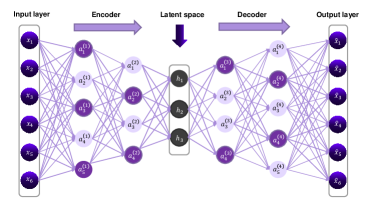
Figure 2: The Sparse Autoencoder Architecture (SAE)

III-A Individual Sparse Autoencoder (SAE)

We first present a single Sparse autoencoder architecture proposed in this paper, which is inspired from [27]. Given an Encoder ($\mathcal{E},\Psi$), a Decoder ($\mathcal{D},\chi$) where $\Psi$ and $\chi$ are the trainable parameters in the Encoder and Decoder respectively, input data $\boldsymbol{x}\in\mathbb{R}^{m}$ is converted into its latent representation with lower dimension $\boldsymbol{h}$ by the Encoder $\mathcal{E}$ via a non-linear mapping:

$$\boldsymbol{h}=\mathcal{E}(\boldsymbol{x};\Psi),\,\,\text{where}\,\,\,\,\,\mathcal{E}(\boldsymbol{x};\Psi)\,:\mathbb{R}^{m}\rightarrow\mathbb{R}^{h},\,h<m$$ (1)

Next, the Decoder $\mathcal{D}$ maps $\boldsymbol{h}$ to a reconstruction sample $\boldsymbol{\overline{x}}\in\mathbb{R}^{m}$ by another non-linear mapping:

$$\boldsymbol{\overline{x}}=\mathcal{D}(\boldsymbol{h},\chi),\,\,\text{where}\,\,\,\mathbf{\mathcal{D}}(\boldsymbol{h};\chi)\,:\mathbb{R}^{h}\rightarrow\mathbb{R}^{m},\,h<m$$ (2)

By constraining the latent space to fewer dimensions than the input space, the trained autoencoder forms a low-dimensional, non-linear manifold that captures the most underlying features of input data. To avoid one problem that normal autoencoders might simply copy or memorize the input data without capturing meaningful features at the latent representation, especially when the number of hidden layers increases [28], [29], a sparse penalty term is added to the cost function. As shown in Fig. 2, the purpose of enforcing sparsity is to limit the undesired activation of the hidden-layer neurons [27], which ensures efficient feature learning at latent space [30], [31].

Consider one sparse autoencoder $\mathcal{A}$, which architecture is represented at Fig. 2. The sparse autoencoder $\mathcal{A}$ has $2L+1$ layers, including one encoder ($\mathcal{E}$) with $L$ layers, one decoder ($\mathcal{D}$) with $L$ layer and one latent layer. We denote $a^{(l)}_{j}$ as the activation of hidden unit $j$ at the $l$-th hidden layer, $z_{j}$ is the input led to that hidden unit $j$. We obtain the average activation of hidden unit $j$ over one batch of $N$ samples, which is written as:

$$\hat{\rho}_{j}=\frac{1}{N}\sum^{N}_{i=1}\left[g\left(a^{(l)}_{j}(z^{(i)}_{j})\right)\right],$$ (3)

where the mapping $g(.)$ uses the sigmoid function, which aims to scale the activation parameter to $[0;1]$ and avoid too large value of $\hat{\rho}_{j}$. The sparity constraint enforces the average activation $\hat{\rho}_{j}$ to the expected value $\hat{\rho}_{j}\approx\rho$, where $\rho$ is the sparsity parameter. The value of $\rho$ is expected to be quite small (close to 0). This facilitates the process of both learning meaningful features and preventing mere copying and memorizing of input data in the context of limited number of activation neurons in the hidden layer as shown in Fig. 2. To achieve the approximation $\hat{\rho}_{j}\approx\rho$, we leverage Kullback–Leibler divergence penalty term [27], which optimizes the difference between two Bernoulli random variable with the means of $\rho$ and $\rho_{j}$, respectively. The KL penalty term applied for the $l$-th hidden layer with $n^{(l)}$ hidden units can be written as:

$$\mathcal{L}^{(l)}_{pen}=\text{KL}(\rho||\hat{\rho}_{j})=\sum^{n^{(l)}}_{j=1}\rho\log{\frac{\rho}{{\hat{\rho}}_{j}}}+(1-\rho)\log{\frac{1-\rho}{1-\hat{\rho}_{j}}}$$ (4)

Then, the penalty term is calculated for all hidden layers of the autoencoder $\mathcal{A}$ (except the latent layer) by taking the sum of KL terms as:

$$\mathcal{L}_{pen}=\sum^{2L}_{l=1}\sum^{n^{(l)}}_{j=1}\rho\log{\frac{\rho}{{\hat{\rho}}_{j}}}+(1-\rho)\log{\frac{1-\rho}{1-\hat{\rho}_{j}}}$$ (5)

We also apply MSE loss for the pair of input data $\boldsymbol{x}$ and reconstruction data $\boldsymbol{\overline{x}}$ for one batch of $N$ samples as:

$$\mathcal{L}_{MSE}=\frac{1}{2N}\sum^{N}_{i=1}||\boldsymbol{x}_{i}-\mathcal{D}\left(\mathcal{E}(\boldsymbol{x}_{i})\right)||^{2}_{2}$$ (6)

Given the KL penalty and MSE losses, we define the final objective function for the optimization of one individual sparse autoencoder $\mathcal{A}$:

$$\mathcal{L}_{SAE}=\mathcal{L}_{MSE}+\beta\mathcal{L}_{pen}$$ (7)

where $\beta$ is the parameter to control the effect of sparsity constraint on the objective function.

III-B k-Sparse Autoencoders

Given the problem of clustering a set of $M$ points $\{\boldsymbol{x}^{(i)}\}^{M}_{i=1}\in\mathbb{R}^{m}$ into $K$ clusters, the classical k-Means algorithm uses a centroid to represents each cluster in the embedding space, the centroids are mostly calculated by taking the average of all points belonging to that cluster. Inspired from [24], [32], we use a set of k-autoencoders to replace the centroids, where each autoencoder represents a cluster and the latent space of one autoencoder is considered as a centroid. In this paper, sparse autoencoders mentioned above are considered as an alternative to normal autoencoders, generating k-Sparse Autoencoders as shown in Fig. 3. Utilizing cluster-specialized sparse autoencoders is a tractable and efficient way to learn features from data points in the same clusters, rather than employing feature learning from a single autoencoder for the entire data [24]. In our deep clustering network, k-Sparse Autoencoders share the same settings and loss function $\mathcal{L}_{SAE}$ in Equation 7.

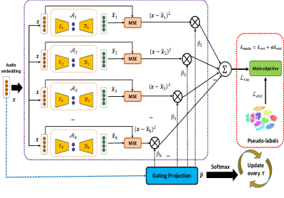
Figure 3: The overall architecture of Mix-SAE

III-C Gating Projection

The role of the Gating Projection ($\mathcal{G}$) is to assign weights $\hat{\boldsymbol{p}}=[\hat{p}_{1},\hat{p}_{2},...,\hat{p}_{k}]$ to the outputs of k-sparse autoencoders based on the input data. Given the weights of $\hat{\boldsymbol{p}}=[\hat{p}_{1},\hat{p}_{2},...,\hat{p}_{k}]$, the Gating Projection is also utilized to assign labels for clusters during the inference phase. In this work, the Gating Projection leverages MLP architecture with a single hidden layer, followed by Leaky ReLU activation and the final softmax layer. Given the input data $\boldsymbol{x}$, the Gating Projection ($\mathcal{G}$) produces weights $\hat{\boldsymbol{p}}=[\hat{p}_{1},\hat{p}_{2},...,\hat{p}_{k}]$ as:

$$\hat{\boldsymbol{p}}=[\hat{p}_{1},\hat{p}_{2},...,\hat{p}_{k}]=Softmax\left(\boldsymbol{W}\boldsymbol{x}+\boldsymbol{b}\right)\in\mathbb{R}^{k}$$ (8)

where $\boldsymbol{W}\in\mathbb{R}^{k\times m},\,\boldsymbol{b}\in\mathbb{R}^{k}$ is the trainable weights and bias of hidden layer in the gating projection.

III-D Training strategy

Concerning the implementation of our proposed Mix-SAE clustering network, the training strategy is briefly represented in Table II, which consists of two steps: Pre-training and Main-training.

Regarding the Pre-training step as shown in Fig. 4, it serves as the parameter initialization scheme for k-sparse autoencoders that is crucial for such non-convex optimization problems unsupervised clustering tasks [24]. The initial pseudo-labels for the entire dataset are also obtained at this stage. Particularly, we follow the strategy described in [24], [32]. We first train a single main sparse autoencoder $\mathcal{A}_{pre}$ as shown in the upper part of Fig. 4, for the entire dataset using the loss function described at equation 7. After training the main sparse autoencoder $\mathcal{A}_{pre}$, one off-the-shelf cluster algorithm (Agglomerative Hierarchical Clustering, K-means, etc) is utilized to obtain initial pseudo-labels $\boldsymbol{{P}}^{[0]}$ from the learned latent representation of the sparse autoencoder $\mathcal{A}_{pre}$. Next, we initialize the parameters of k-sparse autoencoders by sequentially training the $i$-th sparse autoencoder $\mathcal{A}_{i}$ with the subset of points such that $\boldsymbol{\boldsymbol{P}}^{[0]}[c=i]$ as shown in the lower part of Fig. 4, where $c$ denotes the cluster index, $i=1,2,...,k$. Notably, the training process of k-sparse autoencoders also use Equation 7 as the loss function.

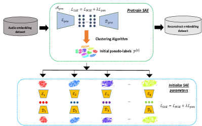
Figure 4: The pre-training step for individual SAE

The next Main-training step is described in Fig. 3. This step involves the joint optimization of the k-sparse autoencoders with initialized parameters obtained from the Pre-training step, and the predicted probabilities from the gating projection. Given k-sparse autoencoders $\{\mathcal{A}_{1}(\theta_{1}),\mathcal{A}_{2}(\theta_{2}),...,\mathcal{A}_{k}(\theta_{k})\}$, where $\theta_{i}=(\Psi_{i};\chi_{i})$ is the parameters of encoder ($\mathcal{E}_{i}$) and decoder ($\mathcal{D}_{i}$) of sparse autoencoder $\mathcal{A}_{i}$, and the parameters ($\boldsymbol{W}$, $\boldsymbol{B}$) of the gating projection $\mathcal{G}$. The main objective function of the proposed Mix-SAE network for one batch of $N$ samples [$\boldsymbol{x}^{(1)},\boldsymbol{x}^{(2)},...,\boldsymbol{x}^{(N)}$] is defined as:

$$\mathcal{L}_{main}(\theta_{1},\theta_{2},...,\theta_{k},\boldsymbol{W},\boldsymbol{B})=\mathcal{L}_{rec}+\alpha\mathcal{L}_{ent}$$ (9)

where $\alpha$ is the parameter to constrain the effect of both terms on the main objective function.

The term $\mathcal{L}_{rec}$ is the weighted sum of reconstruction error over k-sparse autoencoders. This term ensures that the sparse autoencoders focus on inter-cluster reconstruction error, rather than just focusing on reconstructing information alone within their own clusters. We can write this term as:

$$\mathcal{L}_{rec}=-\frac{1}{N}\sum^{N}_{i=1}\sum^{k}_{j=1}\hat{p}^{(i)}_{j}\exp{\left[-\frac{1}{2}\left(\boldsymbol{x}^{(i)}-\mathcal{D}_{i}(\mathcal{E}_{i}(\boldsymbol{x}^{(i)}_{j}))\right)^{2}\right]}$$ (10)

$$~{}~{}~{}~{}~{}~{}~{}~{}~{}~{}~{}~{}~{}~{}\textrm{s.t.}~{}~{}\sum^{k}_{j=1}\hat{p}^{(i)}_{j}=1,\quad\forall i=1,2,\ldots,N.$$

where $\boldsymbol{x}^{(i)}_{j}$ is the output of the $j$-th sparse autoencoder given the input sample $\boldsymbol{x}^{(i)}$; the probability $\hat{p}^{(i)}_{j}$, which is computed from ($\boldsymbol{W}$, $\boldsymbol{B}$) in Equation 8, is the weight assigned to $\boldsymbol{x}^{(i)}_{j}$ from the gating projection.

The term $\mathcal{L}_{ent}$ is referred to as the pseudo-label guided supervision loss. Given the pseudo-labels for one batch of $N$ samples at the time step $t$: $\mathcal{\mathbf{P}}^{[t]}=[\boldsymbol{p}^{[t]}_{1},\boldsymbol{p}^{[t]}_{2},...,\boldsymbol{p}^{[t]}_{N}]$, where $\boldsymbol{p}^{[t]}_{i}\in\mathbb{R}^{k}$, we use the Cross-Entropy loss between the pseudo-labels $\boldsymbol{p}^{[t]}$ updated at time step $t$ and the prediction of the gating projection $\hat{\boldsymbol{p}}^{[t+\Delta t]}$ at the current step $t+\Delta t$:

$$\mathcal{L}_{ent}=-\frac{1}{N}\sum^{N}_{i=1}\boldsymbol{p}^{[t]}_{i}\log{\hat{\boldsymbol{p}}^{[t+\Delta t]}_{i}}$$ (11)

The loss $\mathcal{L}_{ent}$ is leveraged with the expectation that if the pseudo-labels are correctly initialized and updated, they can provide additional guided learning signals by mimicking a semi-supervised setting. This is effective in guiding the model toward the correct cluster results and empowering the learning of meaningful features [33]. During the optimization of the main objective function (9), the pseudo-labels are periodically updated after $\tau$ time step via the prediction of the gating projection at the current step. This action aims to bolster the reliable pseudo-labels indicated by the concurrent minimization of the reconstruction term and the supervision term, while re-correcting the previous noisy pseudo-labels via the control of the reconstruction term. In other words, pseudo-labels are updated over time and act as a form of weak supervision. After the Main-training step, final cluster label can be inferred via the gating projection $\mathcal{G}$. Given each data sample $\boldsymbol{x}$, the probability vector $\hat{\boldsymbol{p}}$ is calculated using equation 8. Then, the cluster label is determined as:

$$\hat{c}=\operatorname*{argmax}\,\hat{\boldsymbol{p}}=\underset{i=1,2,..k}{\operatorname*{argmax}}\,\hat{p}(c=i|\boldsymbol{x})$$ (12)

TABLE II: Mix-SAE Deep Clustering Network

Algorithm 1: Mix-SAE mini-batch training strategy

Input: One batch of $N$ points $\boldsymbol{X}$=$\{\boldsymbol{x}^{(i)}\}^{N}_{i=1}\in\mathbb{R}^{m}$.

Output: One of $k$ cluster labels for $N$ input points.

Components:

- A set of k-autoencoders: $\{\mathcal{A}_{1},\mathcal{A}_{2},...,\mathcal{A}_{k}\}$

$\boldsymbol{x}\rightarrow\bar{\boldsymbol{x}}^{(i)}=\mathcal{D}(\mathcal{E}(\boldsymbol{x})),\,\,\,\,\,i=1,2,...,k.$

- The Gating Projection $\mathcal{G}$ that produces pseudo-labels and

assigns input to suitable autoencoders.

$\boldsymbol{p}=Softmax(\boldsymbol{W}\boldsymbol{x}+\boldsymbol{b})\in\mathbb{R}^{c}$.

Pre-training:

- Train a single autoencoder $\mathcal{A}_{pre}$ for the entire dataset with the

objective function (7).

- Use one off-the-shelf cluster algorithm to initialize pseudo-labels

$\boldsymbol{P}^{[0]}$ for the entire dataset.

for $i=1$ to $k$ do:

Train $i$-th sparse autoencoder with data points $\boldsymbol{P}^{[0]}[c=i]$.

end for

Main-training:

for $t=1$ to $T$ do:

Train the set of k sparse auencoders and the gating

projection $\mathcal{G}$ in parallel using the main objective function (9).

if $t$ mod $\tau=0$ then:

Update new pseudo-labels $\boldsymbol{P}_{new}$ for the batch $\boldsymbol{X}$:

$\hat{\boldsymbol{P}}=Softmax(\boldsymbol{W}\boldsymbol{X}+\mathbf{b})$

$\boldsymbol{P}_{new}\leftarrow\operatorname*{argmax}(\hat{\boldsymbol{P}})$

Get final cluster result: Get the final cluster result for the

batch $\boldsymbol{X}$ via the gating projection $\mathcal{G}$:

$\hat{\boldsymbol{P}}=\underset{\text{axis = 1}}{\operatorname*{argmax}}\left[Softmax\left(\boldsymbol{W}\boldsymbol{X}+\boldsymbol{B}\right)\right]$

TABLE III: Diarization Error Rate (DER) (%) (Collar = 0.0) of Different Systems on SD-EVAL dataset (Whisper version: Tiny)

	$W=0.2$ s				$W=0.4$ s				$W=0.6$ s				$W=0.8$ s				$W=1.0$ s
Methods	EN	FR	GER	SPA	EN	FR	GER	SPA	EN	FR	GER	SPA	EN	FR	GER	SPA	EN	FR	GER	SPA
k-Means	44.77	51.42	49.11	48.25	43.75	51.92	43.84	47.08	38.72	46.88	40.97	42.77	40.23	46.61	44.11	44.38	42.06	47.72	46.13	44.66
AHC	38.42	46.72	41.41	42.93	47.64	52.81	46.33	50.69	40.50	48.69	42.90	43.15	38.55	45.91	43.02	43.44	42.91	47.81	47.63	44.80
SpectralNet [34]	36.18	44.62	40.02	46.03	40.44	51.63	41.22	47.52	37.06	44.68	41.29	42.69	36.11	44.67	44.16	46.42	41.88	46.08	44.31	47.23
DCN [35]	32.15	35.77	36.51	36.98	37.42	38.92	42.17	43.01	32.08	37.57	38.84	40.77	33.02	43.72	44.23	40.55	40.17	45.96	40.21	38.51
DAMIC [24]	27.78	36.22	36.93	35.21	27.97	35.96	36.14	35.11	28.11	36.67	34.66	33.31	27.22	36.91	34.78	34.22	26.95	36.91	36.11	34.65
k-DAE [32]	29.12	37.91	41.23	37.00	30.53	39.81	37.10	37.29	32.72	38.84	34.96	35.23	33.33	38.55	34.24	35.51	30.36	37.32	36.22	35.02
Mix-SAE w/o pen loss	32.18	38.61	36.07	36.78	29.02	35.92	36.51	35.04	27.28	37.01	34.98	34.03	27.90	37.51	34.42	33.83	28.00	37.88	36.18	34.29
Mix-SAE w/o pseudo	28.72	43.22	40.66	36.32	29.62	40.07	36.71	35.72	27.81	36.83	34.90	33.54	27.98	39.68	34.62	33.21	27.93	38.05	36.73	33.82
Mix-SAE	26.51	36.12	35.00	34.91	26.88	37.30	35.64	34.33	27.08	36.70	34.55	32.82	27.24	38.39	34.17	32.03	26.85	37.57	35.33	33.82

IV Experiments Settings And Results

IV-A Evaluating Datasets

To evaluate our proposed system, we collect data from CALLHOME [36, 37, 38] and CALLFRIEND [39, 40] corpora to perform the evaluating dataset. These are benchmark corpora constituted by the Linguistic Data Consortium (LDC) for the project of Large Vocabulary Conversational Speech Recognition (LVCSR) and Language Identification (LID), respectively. Each corpus consists of several language subsets such as English, German, French, Spanish, Japanese, etc. Each language subset includes multiple telephone conversations from various sources in practice. Regarding the evaluating dataset in this work, referred to as SD-EVAL, we gather a portion of data from two-speaker subsets of the two mentioned benchmark corpora as two-speaker conversation is the most common case in telephone call applications. The SD-EVAL dataset consists of 127 audio recordings with a total length of approximately 6.35 hours. The dataset is divided into four subsets, each representing a popular European language: English, Spanish, German, and French. Each subset contains between 25 and 35 audio recordings, with durations ranging from 2 to 5 minutes.

IV-B Evaluation Metrics

We evaluated the proposed network with diarization error rate (DER), which can be defined as:

$$\text{DER}=\frac{\text{FA}+\text{MS}+\text{CE}}{\text{total duration}}$$ (13)

where the false alarm (FA) is the speech incorrectly detected; the missed error (MS) is the speech in the reference that does not represent in the system inference; the confusion error (CE) is the mismatch between the cluster label and the reference. All these terms are calculated in seconds. The final DER score for each language in this work is the average of the DER score of all samples in the corresponding subset.

IV-C Experiment Settings

The proposed method was implemented with deep learning framework PyTorch [41]. All the hidden layers (except the output layer of the gating projection) use Leaky ReLU (with a negative slope of 0.01) as activation function. Both the main autoencoder $\mathcal{A}_{pre}$ at the pretraining-step and the set of k-sparse autoencoders $\{\mathcal{A}_{1},\mathcal{A}_{2},...,\mathcal{A}_{k}\}$ share the similar DNN architecture with the hidden layers of [256, 128, 64, 32] for the encoder and the mirrored version of these for the decoder, followed by Batch Normalization layer after each hidden layer. The latent vector of all the sparse autoencoders has the size of $k$. The mini-batch size $m$ is 16. The sparity parameter $\rho$ is fixed to 0.2. We use k-Means++ [42] as the off-the-shelf clustering algorithm to obtain initial pseudo-labels at the pre-training step.

In terms of tuning hyperparameters on the loss functions, the sparsity constraint parameter $\beta$ for training one sparse autoencoder at equation (7) is set to 0.01. Meanwhile, the parameter to control the pseudo-label supervision loss $\alpha$ at equation (9) is set to 1.

Regarding the training parameters, all the experiments use the learning rate of 0.001, with a weight decay rate of $5.10^{-4}$. At the pre-training step, the main autoencoder $\mathcal{A}_{pre}$ is trained for 50 epochs, followed by 20 epochs for initializing parameters of each of k-sparse autoencoders. At the main-training step, the network is optimized for 20 epochs, while the periodical update of pseudo-labels $\tau$ is performed after 10 epochs.

IV-D Results and Discussion

Speaker clustering methods: Given the speaker embeddings extracted from the tiny Whisper model, we first evaluate the performance among various clustering methods: k-Means, Agglomerative Hierarchical Clustering (AHC), spectral-based network (SpectralNet) [34], autoencoder-based systems such as DCN [35], DAMIC [24], k-DAE [32], and our proposed Mix-SAE. Experiments are conducted on five different segment size values of $W$ (from 0.2s to 1.0s). As experimental results shown in Table III, our proposed Mix-SAE outperforms other clustering methods in most cases of segment size $W$. Our proposed system achieves the best results in English with DER error of 26.51%. It is obviously based on high-quality English speaker embeddings from Whisper model which was trained on a large portion of English data. On the one hand, while other clustering methods are relatively influenced by segment size $W$, especially autoencoder-based methods using the same pre-training strategy such as DCN, k-DAE, our proposed Mix-SAE exhibits stable performances across various values of $W$ (e.g. the system achieves DER scores of 26.51%, 26.88%, 27.08%, 27.24%, 26.85% on English and 35.00%, 35.64%, 35.55%, 34.17%, 34.55% on German with $W$ = 0.2, 0.4, 0.6, 0.8, 1.0, respectively). This indicates the superior efficiency of Mix-SAE network architecture to other autoencoders in capturing speaker features within variable-length segments.

For an ablation study, we establish two other systems: Mix-SAE w/o pen loss (Mix-SAE without sparsity loss in equation 7), Mix-SAE w/o pseudo (Mix-SAE w/o pseudo-label loss in equation 9). Results in Table III demonstrate the role of both sparsity loss and pseudo-label loss in improving the overall performance. For instance, an improvement of 5.67% and 2.21% is obtained in the case of English with $W$ = 0.2s when Mix-SAE is compared to Mix-SAE w/o pen loss and Mix-SAE w/o pseudo, respectively.

The quality of speaker embeddings: We evaluate the effect of the speaker embeddings on the performance. Fig. 5 shows an example of the diarization performance when leveraging speaker embeddings from different versions of Whisper model (Tiny, Base, Small, Medium and Large) with the case of English and $W$ set to 0.2s. It is observable that the superior speaker embeddings are extracted from the larger Whisper models, resulting in the better performance that we can achieve. The best DER score of 17.75% (with a tolerance collar of 0.25s) indicates the promising potential of our approach when leveraging the general-purpose Whisper model to develop multilingual and unsupervised-based speaker diarization systems.

The model complexity: Fig. 6 represents the speaker diarization results (DER) versus the model complexity across deep clustering methods. Our proposed Mix-SAE represents a trade-off between performance and parameter usage (334k parameters with 26.51% DER score). Additionally, when combined with Whisper Tiny version (39M), our speaker diarization system is potential to be integrated into edge devices for sound-based IoT systems [43, 44].

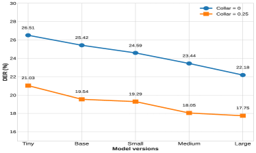
Figure 5: Evaluate the quality of audio embeddings extracted from different Whisper versions (Language: English, $W$ = 0.2s)

Visualization and the effect of Pre-training step: We visualized 2-speaker embeddings after the Pretraining step in our Mix-SAE by applying t-SNE. As Fig. 7 shows, the sparse autoencoders effectively learn underlying patterns from extracted speaker embeddings and map them into latent space where the embeddings of two speakers were relatively well separated. These clustering results serve as pseudo-labels for optimizing the deep clustering network at the next Main-training step.

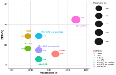
Figure 6: Compare the performance and the model complexity of different deep clustering networks on English evaluation set with $W$ = 0.2s (Whisper version: Tiny)

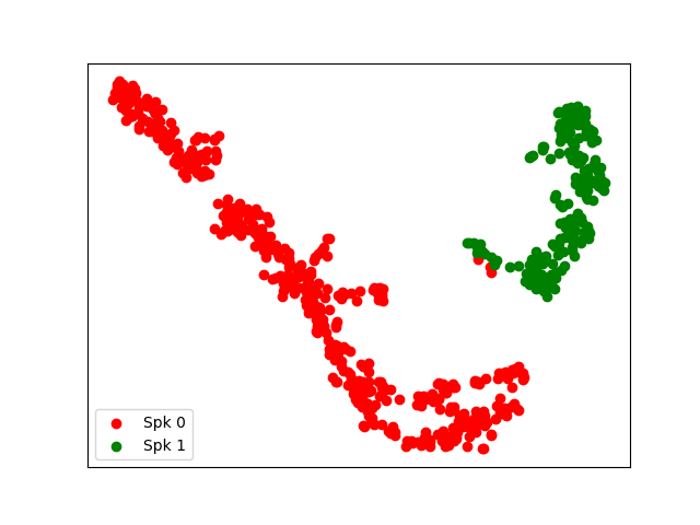
(a) English ($W=0.2s$)

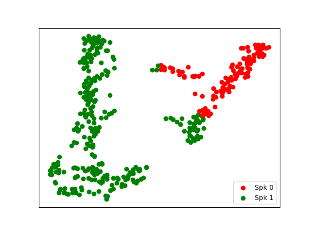
(b) French ($W=0.2s$)

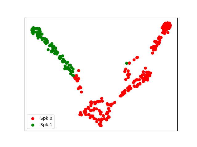
(c) German ($W=0.2s$)

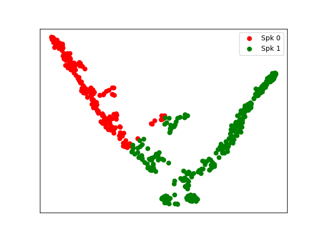
(d) Spanish ($W=0.2s$)

Figure 7: t-SNE visualization of speaker embeddings after the pre-training step (Whisper version: Tiny)

V Conclusion

This paper has presented an unsupervised speaker diarization system utilizing a cluster-based pipeline for multilingual telephone call applications. In this proposed system, the traditional feature extractor was replaced with the Whisper encoder, benefiting from its robustness and generalization on diverse data. Additionally, the Mix-SAE network architecture was also proposed for speaker clustering. Experimental results demonstrate that our Mix-SAE network outperforms other compared clustering methods. The overall performance of our system not only highlights the effectiveness of our approach to unsupervised speaker diarization in the contexts of limited annotated data but also enhances its integration into general-purpose model-based comprehensive multi-task speech analysis application. This work indicates a promising direction toward developing generalized speaker diarization systems based on general-purpose models in future work.

References

- [1] Lam Pham, Tin Nguyen, Phat Lam, Dat Ngo, Anahid Jalali, and Alexander Schindler, “Light-weight deep learning models for acoustic scene classification using teacher-student scheme and multiple spectrograms,” in 4th International Symposium on the Internet of Sounds, 2023, pp. 1–8.
- [2] Lam Pham, Khoa Tran, Dat Ngo, Hieu Tang, Son Phan, and Alexander Schindler, “Wider or deeper neural network architecture for acoustic scene classification with mismatched recording devices,” in Proceedings of the 4th ACM International Conference on Multimedia in Asia, 2022, pp. 1–5.
- [3] Lam Pham, Dat Ngo, Dusan Salovic, Anahid Jalali, Alexander Schindler, Phu X. Nguyen, Khoa Tran, and Hai Canh Vu, “Lightweight deep neural networks for acoustic scene classification and an effective visualization for presenting sound scene contexts,” Applied Acoustics, vol. 211, pp. 109489, 2023.
- [4] Thi Ngoc Tho Nguyen et al., “A general network architecture for sound event localization and detection using transfer learning and recurrent neural network,” in IEEE International Conference on Acoustics, Speech and Signal Processing (ICASSP), 2021, pp. 935–939.
- [5] Ian Mcloughlin, Yan Song, Lam Dang Pham, Ramaswamy Palaniappan, Huy Phan, and Yue Lang, “Early detection of continuous and partial audio events using cnn,” in Proc. INTERSPEECH, 2018.
- [6] Tin Nguyen, Lam Pham, Phat Lam, Dat Ngo, Hieu Tang, and Alexander Schindler, “The impact of frequency bands on acoustic anomaly detection of machines using deep learning based model,” arXiv preprint arXiv:2403.00379, 2024.
- [7] Mohammad Hasanzadeh Mofrad et al., “Speech recognition and voice separation for the internet of things,” in Proceedings of the 8th International Conference on the Internet of Things, 2018, pp. 1–8.
- [8] Luca Turchet et al., “The internet of sounds: Convergent trends, insights, and future directions,” IEEE Internet of Things Journal, vol. 10, no. 13, pp. 11264–11292, 2023.
- [9] Tae Jin Park, Naoyuki Kanda, Dimitrios Dimitriadis, Kyu J Han, Shinji Watanabe, and Shrikanth Narayanan, “A review of speaker diarization: Recent advances with deep learning,” Computer Speech & Language, vol. 72, pp. 101317, 2022.
- [10] Luca Serafini et al., “An experimental review of speaker diarization methods with application to two-speaker conversational telephone speech recordings,” Computer Speech & Language, vol. 82, pp. 101534, 2023.
- [11] Rashmi Gangadharaiah et al., “A novel method for two-speaker segmentation,” in Proc. INTERSPEECH, 2004.
- [12] Alain Tritschler and Ramesh A. Gopinath, “Improved speaker segmentation and segments clustering using the bayesian information criterion,” in EUROSPEECH, 1999.
- [13] Douglas A. Reynolds, Thomas F. Quatieri, and Robert B. Dunn, “Speaker verification using adapted gaussian mixture models,” Digital Signal Processing, vol. 10, no. 1, pp. 19–41, 2000.
- [14] Najim Dehak et al., “Front-end factor analysis for speaker verification,” IEEE Transactions on Audio, Speech, and Language Processing, vol. 19, no. 4, pp. 788–798, 2011.
- [15] Li Wan, Quan Wang, Alan Papir, and Ignacio Lopez Moreno, “Generalized end-to-end loss for speaker verification,” 2020.
- [16] David Snyder et al., “X-vectors: Robust dnn embeddings for speaker recognition,” in IEEE International Conference on Acoustics, Speech and Signal Processing (ICASSP), 2018, pp. 5329–5333.
- [17] Kyu Jeong Han and Shrikanth S. Narayanan, “A robust stopping criterion for agglomerative hierarchical clustering in a speaker diarization system,” in Proc. INTERSPEECH, 2007.
- [18] Aonan Zhang, Quan Wang, Zhenyao Zhu, John Paisley, and Chong Wang, “Fully supervised speaker diarization,” 2019.
- [19] Themos Stafylakis, Vassilis Katsouros, and George Carayannis, “Speaker Clustering via the mean shift algorithm,” in Proceedings of the Speaker and Language Recognition Workshop (Speaker Odyssey), Brno, Czech Republic, 2010, ISCA, pp. 186 – 193.
- [20] Rosanna Milner and Thomas Hain, “Dnn-based speaker clustering for speaker diarisation,” in Proc. INTERSPEECH, 2016.
- [21] Monisankha Pal et al., “Speaker diarization using latent space clustering in generative adversarial network,” in IEEE International Conference on Acoustics, Speech and Signal Processing (ICASSP), 2020, pp. 6504–6508.
- [22] Yanxiong Li, Wucheng Wang, Mingle Liu, Zhongjie Jiang, and Qianhua He, “Speaker clustering by co-optimizing deep representation learning and cluster estimation,” IEEE Transactions on Multimedia, vol. 23, pp. 3377–3387, 2020.
- [23] Alec Radford et al., “Robust speech recognition via large-scale weak supervision,” in International Conference on Machine Learning, 2023, pp. 28492–28518.
- [24] Shlomo E. Chazan, Sharon Gannot, and Jacob Goldberger, “Deep clustering based on a mixture of autoencoders,” in 29th International Workshop on Machine Learning for Signal Processing (MLSP), 2019, pp. 1–6.
- [25] Brian McFee, Colin Raffel, Dawen Liang, Daniel PW Ellis, Matt McVicar, Eric Battenberg, and Oriol Nieto, “librosa: Audio and music signal analysis in python.,” in SciPy, 2015, pp. 18–24.
- [26] Moreno La Quatra et al., “Vad - simple voice activity detection in python,” [Online]. Available: https://github.com/MorenoLaQuatra/vad.
- [27] Andrew Ng et al., “Sparse autoencoder,” CS294A Lecture notes, vol. 72, no. 2011, pp. 1–19, 2011.
- [28] Shuyang Wang, Zhengming Ding, and Yun Fu, “Feature selection guided auto-encoder,” Proceedings of the AAAI Conference on Artificial Intelligence, vol. 31, no. 1, Feb. 2017.
- [29] Zhao Kang, Xiao Lu, Jian Liang, Kun Bai, and Zenglin Xu, “Relation-guided representation learning,” 2020.
- [30] Hoagy Cunningham et al., “Sparse autoencoders find highly interpretable features in language models,” 2023.
- [31] Devansh Arpit, Yingbo Zhou, Hung Ngo, and Venu Govindaraju, “Why regularized auto-encoders learn sparse representation?,” 2016.
- [32] Yaniv Opochinsky, Shlomo E. Chazan, Sharon Gannot, and Jacob Goldberger, “K-autoencoders deep clustering,” in IEEE International Conference on Acoustics, Speech and Signal Processing (ICASSP), 2020, pp. 4037–4041.
- [33] Zeping Min, Qian Ge, and Cheng Tai, “Why the pseudo label based semi-supervised learning algorithm is effective?,” 2023.
- [34] Uri Shaham, Kelly Stanton, Henry Li, Boaz Nadler, Ronen Basri, and Yuval Kluger, “Spectralnet: Spectral clustering using deep neural networks,” 2018.
- [35] Bo Yang, Xiao Fu, Nicholas D. Sidiropoulos, and Mingyi Hong, “Towards k-means-friendly spaces: Simultaneous deep learning and clustering,” 2017.
- [36] Canavan Alexandra, David Graff, and George Zipperlen, “Cabank english callhome corpus,” 1997, doi: 10.21415/T5KP54.
- [37] Alexandra Canavan, David Graff, and George Zipperlen, “Cabank german callhome corpus,” 1997, doi: 10.21415/T56P4B.
- [38] Canavan Alexandra, David Graff, and George Zipperlen, “Cabank spanish callhome corpus,” 1996, doi: 10.21415/T51K54.
- [39] Lorenza Mondada et al., “Cabank french callfriend corpus,” doi: 10.21415/T5T59N.
- [40] Lorenza Mondada and Tania Granadillo, “Cabank spanish callfriend corpus,” doi: 10.21415/T5ZC76.
- [41] Adam Paszke et al., “Pytorch: An imperative style, high-performance deep learning library,” in Advances in Neural Information Processing Systems 32, pp. 8024–8035. Curran Associates, Inc., 2019.
- [42] David Arthur and Sergei Vassilvitskii, “k-means++: the advantages of careful seeding,” in Proceedings of the Eighteenth Annual ACM-SIAM Symposium on Discrete Algorithms, USA, 2007, SODA ’07, p. 1027–1035, Society for Industrial and Applied Mathematics.
- [43] Iván Froiz-Míguez et al., “Design, implementation, and practical evaluation of a voice recognition based iot home automation system for low-resource languages and resource-constrained edge iot devices: A system for galician and mobile opportunistic scenarios,” IEEE Access, vol. 11, pp. 63623–63649, 2023.
- [44] Andrés Ramírez and Mary Ellen Foster, “A whisper ros wrapper to enable automatic speech recognition in embedded systems,” 2023.