The University of Sydneyjoachim.gudmundsson@sydney.edu.auhttps://orcid.org/0000-0002-6778-7990 Funded by the Australian Government through the Australian Research Council DP180102870. The University of Sydneyzijin.huang@uni.sydney.edu.auhttps://orcid.org/0000-0003-3417-5303 The University of Sydneyandre.vanrenssen@sydney.edu.auhttps://orcid.org/0000-0002-9294-9947 The University of Copenhagensawo@di.ku.dkhttps://orcid.org/0000-0003-3803-3804
Acknowledgements.
\CopyrightJoachim Gudmundsson, Zijin Huang, André van Renssen and Sampson Wong \ccsdescTheory of computation Computational geometrySpanner for the weighted region problem
Abstract
We consider the problem of computing an approximate weighted shortest path in a weighted subdivision, with weights assigned from the set . We present a data structure , which stores a set of convex, non-overlapping regions. These include zero-cost regions (0-regions) with a weight of and obstacles with a weight of , all embedded in a plane with a weight of . The data structure can be constructed in expected time , where is the total number of regions, represents the total complexity of the regions, and is the approximation factor, for any . Using , one can compute an approximate weighted shortest path from any point to any point in time. In the special case where the 0-regions and obstacles are polygons (not necessarily convex), contains a -spanner of the input vertices.
keywords:
weighted region problem, approximate shortest path, spanner1 Introduction
The Weighted Region Problem (WRP) is a generalization of the shortest path problem, considering a planar subdivision where each face has a non-negative weight associated with it. A path in can be partitioned into a set of subpaths based on its intersection with faces in , where a subpath starts at the point and ends at the point . Both and must lie on the boundary of the same face . The weight of the subpath is the Euclidean length of times the weight assigned to . The total weight of a path is the sum of the weights of its subpaths. The goal of the WRP is to find the weighted shortest path from a source point to a target point . When the weights are in the set , this problem is referred to as the Weighted Region Problem [17].
Researchers have conjectured that the WRP is difficult to solve [17], and recent studies confirm this conjecture — the Weighted Region Problem is unsolvable in the algebraic computation model over the rational numbers. De Carufel et al. [14] demonstrated that the WRP cannot be solved exactly even with only three different weights. De Berg et al. [12] confirmed its unsolvability with just two different weights. Mitchell and Papadimitriou [21] illustrated that in two dimensions, a weighted shortest path can intersect at least boundaries even when the regions are convex.
Due to the difficulty of solving the WRP exactly, approximation algorithms have been considered. A common approach is to discretize the problem space, either by assuming the space is a tessellation of convex polygons with exactly one associated weight [5], or by placing Steiner (sample) points on the boundaries of the regions [1, 2, 9, 20, 23]. In these approaches, the number of sample points depends not only on the complexity of the regions but also on geometric parameters such as the maximum integer coordinate of any vertex and the ratio of the maximum weight over the minimum weight. As increases, so does the number of required sample points. As a result, the weights are required to be strictly positive.
1.1 Related work
Our work is closely related to the data structure and algorithm by Gewali et al. [17] to solve the weighted region problem. Their algorithm takes a polygonal domain with vertices as input and constructs a critical graph (a type of visibility graph) with edges. Dijkstra’s shortest path algorithm can be used on to compute a weighted shortest path between any pair of vertices in time.
In weighted regions, a weighted shortest path avoids obstacles and traverses the 0-regions freely, while minimizing its length in the plane (-region). Consider two (closed) regions and , each either a 0-region or an obstacle. The key observation in [17] is that an edge in connecting and must be locally optimal (see Fact 2). For example, an edge connecting two convex 0-regions and must be perpendicular to the tangent touching and the tangent touching . Gewali et al. [17] showed that contains all such locally optimal edges in , which implies that must contain the optimal path between any pair of vertices in .
1.2 Our Contribution
In this paper, we build on the work by Gewali et al. [17] with a focus on the -regions as they are not handled well by existing approximation schemes (using sample points or tessellation). In Section 2, we consider the weighted region problem where the 0-regions are convex but not necessarily polygonal.
Problem 1.
In the planar subdivision induced by the plane with weight and a set of non-overlapping convex zero-cost regions (0-regions) with weight , given an approximation error , find a -approximate weighted shortest path from an arbitrary point to an arbitrary point .
The high-level idea is that, in order to obtain -approximate shortest paths, we place sample points on the boundary of each -region; the number of sample points is independent of other parameters. Using these sample points, we construct a -graph and trapezoidal maps, which are part of our data structure . The trapezoidal maps ensure the existence of good paths between -regions that are close111A precise definition is provided in Lemma 2.4 and 2.8, Section 2. to each other, while the -graph ensures the same for -regions that are far from each other. To the best of our knowledge, our algorithm is the first near-linear time -approximation algorithm that finds an approximated weighted shortest path in a weighted region. Our algorithm is near-optimal, as a weighted shortest path can have complexity.
Theorem 1.1.
Consider a planar subdivision induced by a plane with weight 1, containing a set of non-overlapping convex 0-regions with weight 0. Let and denote the total number of vertices in . For any approximation factor , a data structure can be constructed over in expected time, with a total size of . When queried with points and , can return a weighted path from to in time, satisfying , where is the optimal weighted shortest path from to .
To use our algorithm on an application, we proved the above theorem in a more general setting, where the 0-regions are non-polygonal. In Section 3, we use our algorithm to approximate the partial weak Fréchet similarity of two polygonal curves. This problem was first studied by Buchin et al. [7], and they presented a cubic time algorithm. De Carufel et al. [13] later transformed the problem into a weighted shortest path problem amidst -regions. Using Theorem 1.1, our algorithm is the first near-quadratic time -approximation algorithm for computing the partial weak Fréchet similarity between a pair of polygonal curves.
Buchin et al. [8] showed that there is no strongly subquadratic time algorithm for approximating the weak Fréchet distance within a factor less than 3 unless the strong exponential-time hypothesis fails. Approximating the partial weak Fréchet similarity is at least as hard as approximating the weak Fréchet distance. As a result, it is unlikely that a subquadratic time algorithm exists, and our algorithm is near-optimal.
Theorem 1.2.
One can approximate the partial weak Fréchet similarity of two curves with respect to the metric within a factor of in expected time.
In Section 4, we generalise our data structure to also allow convex obstacles that cannot be traversed, i.e., obstacles of weight . By introducing additional sample points, we show that if we need to take a detour from a sample point to a sample point , there exists a set (a detour) of edges in such that the total length of approximates the distance within a factor of . In the special case that the 0-regions and obstacles are polygonal, is a -spanner of the input vertices. To the best of our knowledge, our algorithm is the first near-linear time -approximation algorithm for the weighted shortest path in a weighted region.
Theorem 1.3.
Consider a planar subdivision induced by a plane with a weight of , consisting of two sets of convex and non-overlapping regions: 0-regions with a weight of , and obstacles with a weight of . Let and let denote be the total number of vertices in . For any approximation factor , a data structure can be constructed over in expected time, with a total size of . When queried with arbitrary points and , returns a weighted path from to in time, ensuring that , where is the optimal weighted shortest path from to .
2 Shortest path amidst 0-regions
The exact version of Problem 1 has a brute-force solution. Given two 0-regions and , where and are considered 0-regions with no interior, let be the Euclidean distance between and . Let be a complete graph, where . For each edge for all pairs of and , set the weight . Then, finding the optimal path from to is equivalent to finding a weighted shortest path in , which can be solved using Dijkstra’s shortest path algorithm. However, the total number of edges required is at least .
To compute an approximate solution, the goal is to construct an undirected weighted graph , with a near-linear number of edges, such that there exists a path in with .
To this end, we will use two data structures: trapezoidal maps and -graphs. Both data structures are used to determine which pairs of 0-regions are connected. The trapezoidal maps will ensure that there exist good paths between 0-regions that are close to each other, while the -graph ensures the same for -regions that are far from each other.
2.1 Construction of the data structure
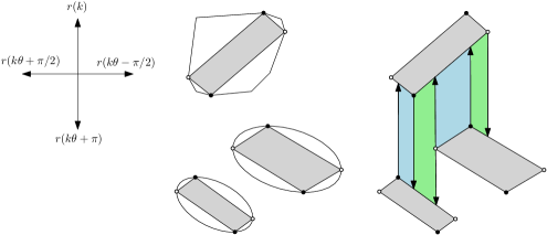
In order to define our data structure, we first define a set of directions. Let be a fixed positive real number. Let be the direction with a counter-clockwise angle of with the positive -axis. Let be the ray originating from the point with a counter-clockwise angle of with the positive -axis. For simplicity, we write and . To simplify the discussion, we will assume that to guarantee that if exists, then so does .
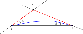
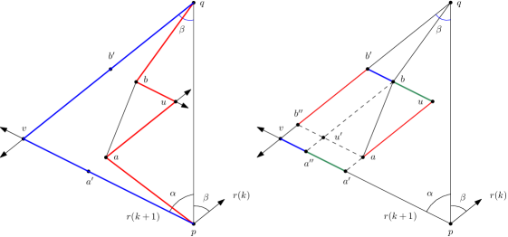
For a 0-region , we define a set of sample points on the boundary of . Let be a sample point on the boundary of such that is extreme in the direction (see Figure 1). When the geometric region is clear from context, we write instead of .
Each 0-region is considered an open set, i.e., if , then . Let define the subset of traversed from point to point in counter-clockwise order, where . We say a line overlaps if and intersect at more than one point. We say two regions, and , are non-overlapping if their interiors do not intersect.
A point can be an extreme point for more than one direction, in which case we call a vertex of . There may be more than one extreme point on for a single direction. If is the extreme point on for consecutive directions , we say , , …, and simultaneously. If there is more than one extreme point for a single direction , these extreme points must lie on some segment , and we say both and are . The sample points on the boundary of a convex region can be computed by traversing the boundary.
Given convex regions with vertices in total, there are sample points, and it takes time to compute them.
Using the sample points on a 0-region , we can generate a simplified -region (a convex polygon) by connecting adjacent sample points of every 0-region (see Figure 1). Using the set of simplified 0-regions, we will generate a set of trapezoidal maps, and we say and are adjacent if they are both adjacent to the same face in a trapezoidal map. We construct the query data structure using Algorithm 1.
This algorithm takes as input a set of non-overlapping and convex 0-regions, and constructs a data structure . The undirected graph is initially empty.
-
1.
Compute the sample points , and add to .
-
2.
Pick an arbitrary sample point as the anchor for every . For each , add to , and set .
-
3.
For each direction , generate a trapezoidal map using , and do the following for each (see [11, Theorem 6.3 and 6.8] for trapezoidal map construction).
-
•
For each face adjacent to and , , add to , and set .
-
•
-
4.
With as the input, generate a -graph .
-
•
For each edge , if and do not belong to the same 0-region, add to , and set .
-
•
-
5.
Return as the data structure.
2.1.1 Analysis
We bound the size of the data structure and its construction time. In Step 1, by Observation 2.1, it takes time to compute all sample points. Step 2 takes time to connect every sample point to its respective anchor. In Step 3, it takes expected time [11] to build the trapezoidal map over for each of the directions. In every , we construct at most three edges in per sample point , if and hit different 0-regions. Therefore , and in total . Once is constructed for all , using the algorithm by Edelsbrunner [15], it takes time to compute the shortest distance between two convex 0-regions for each of the faces. In Step 4, it takes time to construct a -graph using sample points, and cones [22]. Step 4a takes time, since .
Later, we will show that for an approximation factor , we have that . The resulting complexities are summarised below.
Lemma 2.1.
Given an approximation factor , and non-overlapping convex 0-regions with total complexity , one can build the data structure in time, and the total size of is .
To the best of our knowledge, constructing a trapezoidal map using arcs has not been studied before. Therefore, in Algorithm 1, we used the well-studied result on the trapezoidal map construction using segments.
For each direction , we built a trapezoidal map using the simplified 0-regions , see Step 3 of Algorithm 1. Consider the union of and . We argue that constructing a trapezoidal map using the simplified regions captures the structure of the trapezoidal map if we had used the subboundaries of the original regions instead. To do this, we show that if a ray originating from a sample point on 0-region hits a subboundary first, then must hit the segment next.
First, the 0-regions are non-overlapping, so cannot intersect the region enclosed by and . Second, without loss of generality, let coincide with the -axis. By construction, if exists, then and exist, which implies that there exist two sample points: one is the leftmost point of , and one is the rightmost. Therefore, the horizontal span of and are equal. A ray shooting in the direction cannot hit first but misses .
If a ray hits a subboundary first, then must hit next.
With the data structure defined, we analyse the quality of the path we obtain from .
2.2 Trapezoidal map
Before arguing that there exists a good path using the edges constructed, we start with an observation about the pair of points realising the shortest distance between two 0-regions. For a convex region and a point , there exists at least one supporting line going through such that lies entirely in one of the two halfplanes determined by [24]. Let , and . We can observe that if realises , then must be perpendicular to a pair of supporting lines and .
Let and be two convex regions. Let be the line segment realising , where and . The segment must be perpendicular to a pair of supporting lines and .
We will show that if realises the distance between two 0-regions, we can transform into another segment such that is parallel to some direction , and approximates . To do this, we first need a fact (see Appendix LABEL:app:lemma_rotation for a proof).
Lemma 2.2.
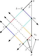
Given a segment , let (resp. ) be the acute angle between and (resp. ), where . Let be the intersection of and . We have that , and .
Proof 2.3.
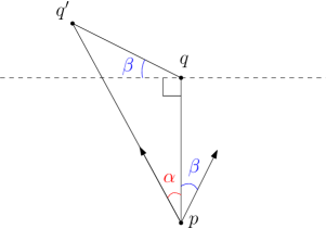
See Figure 2 for the construction. By the law of sines, we have
Filling in our angles, we get
Similarly, by the law of sines, we have
Filling in our angles, we get
The proof is complete.
Let realise . We consider the scenario when is relatively small compared to the horizontal span of (say) . Using the above lemma, we will show that we have constructed a set of edges in connecting two sample points and , such that the total weight of these edges approximates .
Lemma 2.4.
Let , and let realise , where and . Let , and , where points and (resp. and ) are adjacent sample points on 0-region (resp. ). If or , then there exists a path from to such that .
Proof 2.5.
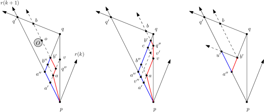
Without loss of generality, assume that . Lemma 2.2 implies that there exists a point such that is in some direction , and .
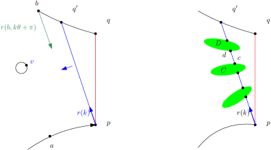
Observe that cannot overlap any 0-region; otherwise, is not optimal. If does not overlap any 0-region (see Figure 3, left), we fix the orientation of , and move along and along , until touches a sample point.
If touches (resp. ), then (resp. ) hits (resp. ). If touches a sample point , must be extreme in the direction . As a result, hits , and hits . In either case, and are adjacent in some face of , and the edge is in by construction. As a result, . This is also trivially true when or is already a sample point.
Otherwise, the segment overlaps a set of 0-regions, and there exists a path from to through (see Figure 3, right). Since the 0-regions do not overlap, the boundaries of the 0-regions in partition into a set of intra-region and inter-region segments. Let be one among the set of inter-region segments, where is on a 0-region , and is on a 0-region . Using the same argument as above, one can slide until it touches a sample point, and edge exists by construction.
In total, traveling from to via the 0-regions must be less costly than , since , and the intra-region segments have weight 0. Summing up the cost of , we have that
2.3 -Graph
In Step 4 of Algorithm 1, we constructed a -graph using the defined sample points. The vertices are simply all sample points. The edges in are constructed using the standard -graph construction [11]. Recall that in Algorithm 1, for every edge , with , , and , we add an edge to , and set .
The -graph constructs a set of “good” edges in when the distances between (resp. ) and its adjacent sample points are small compared to . In this case, we argue that there exists a pair of sample points and , such that . Similar to Lemma 2.2, we first prove a geometric property.
Lemma 2.6.
Given a segment , let (resp. ) be the acute angle between and (resp. ), where . Let be the intersection of and , and let be the intersection of and . Let be the intersection of and . We have that , and .
Proof 2.7.

See Figure 4 for the construction. Without loss of generality, assuming . Using the law of sines in the triangle , we have the following.
| (1) |
Observe that , since is the result of rotating counter-clockwise by . Therefore, is a right triangle, and we have the following.
Using an analogous computation, we obtain
Combining and , we have that
| (2) |
Next, since is a right triangle, we can bound as follows.
Since , all terms are greater than 0, and .
In the case that both and are close to their adjacent sample points, we argue that there exists a pair of sample points such that approximates .
Lemma 2.8.
Let , and let realise , where and . Let , and , where points and (resp. and ) are adjacent sample points on (resp. ). If and , then .
Proof 2.9.
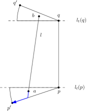
We argue that (see Figure 5), where (resp. ) is the intersection of (resp. ) and (resp. ). Let (resp. ) be the intersection of (resp. ) and (resp. ). Without loss of generality, assume is parallel to the -axis, and , and consider the sample point next to counter-clockwise.
We will first show that must reside in a circular sector. The region is convex; therefore must be below the supporting line . Due to how the sample points are constructed, the sample point must be above . Since , must reside in the disk centered at with radius . Combining the above restrictions, we have that must reside in the smaller circular sector of enclosed by and . An analogous argument shows that must reside in the smaller circular sector of enclosed by and .
Consider the line through , and observe that pushing along towards the boundary of strictly increases . Next, now that lies on the boundary of , we push towards along the boundary of . This also increases , since . Now that , an analogous argument applies to , since . In conclusion, .
By Lemma 2.6, , and the proof is complete.
2.4 The quality of the path
For now, assume that and lie in some 0-region. An optimal - path consists of a set of segments, where the endpoints of each segment lie on the boundaries of the 0-regions. A segment either lies within a 0-region or connects two different 0-region. Since it costs nothing to follow an edge inside a 0-region, the weight of is the total weight of those edges connecting different 0-regions.
Let realise the distance between 0-regions and , where lies on between sample points and , and lies on between sample points and . In Lemma 2.4, we have shown that if or , there exists a path from a sample point on to a sample point on of length at most .
In Lemma 2.8, we have shown that if and , there exist sample points and , such that . To obtain a path between and in this case, we rely on the -graph. The tightest bounds on the length of this path are due to Bose et al. [4], who showed that the spanning ratio of a -graph is at most .
In summary, if , there exists a path from to such that
Given an approximation factor , we compute a proper value for as follows.
Using , we can construct the data structure . Combining Lemma 2.4 and Lemma 2.8, we have the following.
Lemma 2.10.
Data structure contains a path from sample point to sample point such that , where is the optimal path from to .
2.5 Finding a shortest path amidst -regions
Now that we know good paths exist between all pairs of sample points, it remains to include our arbitrary query points and . Given the data structure , a point , and a point , we query the approximate shortest path from to using Algorithm 2.
This algorithm takes as input a point and a point , and a data structure storing a set of 0-regions. It outputs an -approximated weighted shortest path from to . In Step 1 and Step 2, this algorithm shows how to add to , and the same operations are used to add .
-
1.
For each trapezoidal map , do the following for point .
-
(a)
Query the face containing .
-
(b)
Let be adjacent to 0-regions and . Add to , and set . Perform the same operation for and .
-
(a)
-
2.
Add to . Specifically, using as the apex, we construct a set of disjoint cones with -angle. For each point closest to in each cone, add to , and set . For every existing vertex , and every existing edge , if is closer to than is, add to , and set . (Note that -graph uses projected distance instead of Euclidean distance.)
-
3.
Use Dijkstra’s shortest path algorithm to compute a path from to in . Transform into a path in the original environment and return .
Once and are added to , they are treated as 0-region with no interior. The point is its extreme point in every direction. Therefore, the distance between and its adjacent sample points is . As a result, Lemma 2.4 and Lemma 2.8 both apply. Thus with and added contains a -approximation of the shortest path from to , which Dijkstra’s shortest path algorithm will find.
2.5.1 Analysis
Finally, we look at the query time. Recall that . In Step 1, we consider trapezoidal maps. For each trapezoidal map, it takes time to perform a point-location query [11], and it takes time to compute [15]. In Step 2, it takes time to find the closest point of in each cone, and at the same time check if is closest to any point . In Step 3, it takes time to run Dijkstra’s shortest path algorithm to find the shortest path from to in [16]. It takes time to transform into a path in the environment. The query time is .
See 1.1
3 Partial weak Fréchet similarity
This section highlights one application of our data structure: approximating the partial weak Fréchet similarity. This problem was previously considered by Buchin et al. [7] and De Carufel et al. [13]. We start with an introduction for the Fréchet distance and the weak Fréchet distance, eventually leading us to the formal definition of the partial weak Fréchet similarity problem.
The Fréchet distance is a popular measure of the similarity between two polygonal curves. An orientation-preserving reparameterisation is a continuous and bijective function such that , and . The between two curves and with respect to the reparameterisations and , is defined as follows.
Consider the scenario where a person is walking his dog with a leash connecting them: the person needs to stay on while walking according to , and the dog needs to stay on while walking according to . The maximum leash length is the width between and with respect to the reparameterisations and . The standard Fréchet distance is the minimum leash length required over all possible walks (defined by reparameterisations and ).
Problems relating to the Fréchet distance are commonly solved in a configuration space called the freespace diagram. The free space with respect to the Fréchet distance is the union of all pairs of points and such that the distance between and is at most . As opposed to the free space, we will call the forbidden space.
The freespace diagram is a data structure that stores the free space in cells. Alt and Godau [3] showed that the intersection of the free space with each cell is the intersection of an ellipse and a rectangle. Therefore the free space in each cell is convex, and its boundary is of constant complexity. For two polygonal curves with complexity , Alt and Godau [3] proved the following fact.
Fact 1.
The freespace diagram contains at most cells, and it can be constructed in time. The free space inside each cell is the intersection of an ellipse and a rectangle.
It is well-known that if one can find an -monotone path in from the bottom-left corner to the top-right corner via the free space, then .
The notion of weak Fréchet distance relaxes the requirement of the reparameterisation : it still needs to be continuous but not bijective. This means that the person and the dog can walk backward. To determine if the weak Fréchet distance is at most , we need to find only a (potentially not -monotone) path through the free space from to in . Buchin et al. [8] showed that there is no strongly subquadratic time algorithm for approximating the weak Fréchet distance within a factor less than 3 unless the strong exponential-time hypothesis fails.
Buchin et al. [7] proposed the partial Fréchet similarity (partial similarity in short) to deal with the Fréchet distance’s sensitivity to outliers. Instead of determining whether a leash of length is enough to complete the walk, partial similarity determines how much can be completed given a leash of length . The partial similarity is the total length of the portion of two curves that are matched under the Fréchet distance .
Let be the distance between point and point under the norm. Let be the norm of the vector . Under the metric, given the desired Fréchet distance , the partial similarity of curves and with respect to the reparameterisations and is formally defined as follows [7].
Naturally, we want to compute a pair of reparameterisations and that maximise the partial similarity. To do this, Buchin et al. [7] proposed a cubic time algorithm. They showed that it is sufficient to find an -monotone path from to such that intersects as much free space as possible, i.e., should be maximised. When the distance measure between two curves is the more natural -metric, De Carufel et al. [13] proposed a cubic time algorithm with an additive error. They showed that finding a path that intersects as much free space as possible is equivalent to finding a path that intersects as little forbidden space as possible. They formalised the latter as the Minimum-Exclusion (MinEx) problem. They also showed that the MinEx problem is equivalent to the weighted shortest -monotone path problem: computing a -monotone weighted shortest path from to in the freespace diagram, where the weight in the forbidden space is one, and the weight in the free space is zero. Under the weak Fréchet distance, the monotonicity requirement is removed.
Therefore, solving the weak Fréchet version of the MinEx problem under the metric is equivalent to finding a weighted shortest path amidst a set of non-overlapping and convex -regions, where each 0-region is of constant complexity. Using Theorem 1.1 and Fact 1, we have the following theorem.
See 1.2
4 Shortest path amidst 0-regions and obstacles
In this section, we generalise our data structure from Section 2 to allow convex obstacles that cannot be traversed, i.e., obstacles with weight . Our problem is finding an approximate shortest path amidst 0-regions and obstacles. More concretely, we consider the following problem.
Problem 4.1.
In the planar-subdivision induced by the plane with weight , and a set of non-overlapping convex regions consisting of obstacles with weight , and -regions with weight , given an approximation error , find a -approximate weighted shortest path from point to point .
In this section, we redefine as the minimum distance between two geometric regions and in a weighted setting. The -graph can be constructed in an environment with obstacles. Clarkson [10] described such construction over points and polygonal obstacles, and proved that a path that -approximates exists in the -graph, where and are vertices. We will use this -graph in the rest of the paper.
Like in the previous section, we will first describe the construction of the data structure and analyse the time and space complexity. We then show that contains a good path between every pair of sample points. We use this to argue the approximation ratio for arbitrary and .
4.1 Construction of the data structure
In order to deal with obstacles, we need to define two new types of sample points. For clarity, we refer to the sample points defined previously as the original sample points. In Section 2, a trapezoidal map was only used to determine if two 0-regions should be connected, and we did not explicitly compute the intersection of a vertical segment and the boundary of a region. With the introduction of obstacles, we do need such intersections. Consider a sample point . When constructing , we shoot two vertical rays from , one upwards and one downwards. Let be the first intersection of with the boundary of some region that is not . We call a propagated sample point.
The other type of sample points we need is the tangent sample points. Given two disjoint obstacles and , and a common tangent , if touches at point and at , we add and as tangent sample points. When we say a point is a sample point, can be any type of sample point.
Recall that is the simplified region by connecting every pair of adjacent sample points of . is the set of simplified 0-regions, and is the set of simplified obstacles. We formally define the construction of our data structure. Given a set of convex obstacles and a set of convex -regions, we build our data structure using Algorithm 3.
This algorithm takes as input a set of non-overlapping and convex regions, including 0-regions and obstacles , and constructs a data structure . The undirected graph is initially empty.
-
1)
Compute the original sample points , and add them to .
-
2)
For each direction , generate a trapezoidal map using .
-
3)
For every , do the following for every face adjacent to and , .
-
(a)
Compute the propagated sample points, and add them to .
-
(b)
If and are both 0-regions, add to , and set .
-
(c)
If at least one of and is an obstacle, let and be the vertical segments defining , where , and . Add edges and to . Set and .
-
(d)
If and are both obstacles, we compute their common tangents. For each common tangent that touches at and at , add and to .
-
(a)
-
4)
Redefine as the polygon generated by connecting adjacent sample points of , original, propagated, and tangent sample points included. With and as the input, generate a -graph .
-
•
For each edge , if and belongs to different regions and , add to and set .
-
•
-
5)
For every pair of adjacent sample points on an obstacle, add to edges, and set .
-
6)
Pick an arbitrary sample point as the anchor for every . For each sample point of a -region , add to , and set .
-
7)
Return as the data structure.
4.1.1 Analysis
Recall that we are given an approximation error and a set of non-overlapping convex regions consisting of obstacles and 0-regions . There are regions, and the total complexity of is . In Step 1, it takes time to compute the sample points. In Step 2, it takes expected time to construct the trapezoidal maps [11].
Step 3 considers trapezoidal map faces. In Step 3a, given a vertical segment intersecting a non-vertical segment , it takes time to use a binary search on to find the intersection of and . In Step 3b, using the algorithm by Edelsbrunner [15], it takes time to compute the distance between two 0-regions. In Step 3c, it takes constant time to compute the length of the vertical segments. In Step 3d, using the algorithm by Kirkpatrick and Snoeyink [19], and Guibas et al. [18], it takes time to compute at most four common tangents. In total, Step 3 takes time, and we add at most tangent and propagated sample points.
In Step 4, using Clarkson’s algorithm [10], it takes time to generate a -graph with obstacles using sample points and cones. In Step 5, it takes time to generate an edge and set the weight for every pair of adjacent sample points. Step 6 takes time to connect every sample point in a 0-region to its anchor.
We generate original sample points. We generate a constant number of propagated and tangent sample points for each of the faces. As a result, each propagated or tangent sample point contributes a constant number of edges in . A -graph constructed with sample points, and cones has at most edges. Therefore . We summarise the complexities below.
Lemma 4.2.
Given an approximation error , and non-overlapping convex regions including -regions and obstacles with total complexity , one can build the data structure in expected time, and the total size of is .
The structure of the rest of the section is as follows. By Lemma 4.3, the distance between two adjacent sample points on the boundary of an obstacle approximates the straight line segment. Therefore, we show that we can “snap” the vertices of an optimal path to our sample points. For every segment , we then argue that either the trapezoidal map or the -graph contains a path approximating to within a factor of .
4.2 Walking on the boundary is not expensive
We first argue that if and are adjacent sample points of , then approximates within a factor of . Therefore, if we find a path amidst the simplified obstacles, we only need to pay a small factor to transform into a path amidst the original obstacles. Then, we prove that if is part of the optimal path, we can replace with a path , such that approximates .
Lemma 4.3.
Let and be adjacent sample points on , where appear after in a counter-clockwise walk. We have that .
Proof 4.4.
See Figure 6. Let be the intersection of and . By convexity of , . By the construction of the sample points, . Let , and let . Then, using the law of sines, we have the following.
The above expression is maximised when , resulting in the following.
The above lemma implies the following. Let be the distance between point and point in the environment with simplified obstacles and simplified 0-regions, and let be the path achieving this distance. If we partition using the sample points, in the worst case, each segment connects adjacent sample points on obstacles. This implies the following corollary.
Corollary 4.5.
Let and be two sample points. We have that .
4.3 Snapping a segment of the optimal path to the sample points
Gewali et al. [17] defined three types of locally optimal edges joining two simple polygonal regions, and they proved that the shortest path from to must be comprised of these locally optimal edges [17, Lemma 2.5] (ignoring edges in 0-regions). For convex obstacles and 0-regions, we need to consider only four types of segments.
Fact 2.
If segment is in the optimal weighted path amidst convex and non-overlapping 0-regions and obstacles, there must exists two supporting lines and such that belong to one of the following cases (ignoring segments in 0-regions).
-
1)
connects two 0-regions such that and .
-
2)
connects the point on a 0-region and the point on an obstacle such that , and .
-
3)
lies on one of the common tangent of two different obstacles.
-
4)
and are two points on the same obstacle, and or .
In Section 4.3.1, 4.3.2, and 4.3.3, we handle each type of edge in Case 1, 2, and 3, respectively. For an edge in each of these cases, we argue that a good path in our data structure approximates . Section 4.4 summarises the approximating ratio using the Case 4 edges.
More specifically, in the following subsections, we argue that for each type of segment , there exists a path constructed using our data structure such that the length of approximates . If is parallel to a direction , based on the construction of the sample points and Fact 2, and are both sample points, and the argument is straightforward. Therefore, we will focus on the scenario where is not parallel to any predefined direction. We assume without loss of generality that lies between the direction and , and (resp. ) is the measure of the acute angle between (resp. ) and . Furthermore, by Corollary 4.5, we consider only simplified obstacles.
4.3.1 Case 1: connects two -regions
We observe that, unfortunately, Lemma 2.4 does not trivially apply. When we rotate to , if overlaps obstacles, a path generated using the skewed set of obstacles can be much longer than , since the path would have to take a detour around the obstacles. The following lemmas resolve this issue.
Lemma 4.6.
Let and be two -regions. Let , where , and . If , where is a sample point adjacent to , then there exists a sample point such that .
Proof 4.7.
In Lemma 2.4, we showed that if , we can transform into . If intersects no obstacles, there exists a path from to such that approximates , which also implies this lemma. Otherwise, intersects at least one obstacle. Without loss of generality, we assume that is aligned with the -axis, where .
First, consider a horizontal ray , and rotate counter-clockwise until the new ray, , hits a sample point on the boundary of some simplified obstacle (see Figure 7, left). Let the counter-clockwise rotation from to be . With and defined, let be the first sample point that is hit by rotating the ray counter-clockwise. We continue this process until either is parallel with direction , or hits a sample point on . Let this final ray be , and hits at a sample point . Indeed, if is in the direction , then hits , and is a propagated sample point.
Similarly, let . We perform the same process starting from . Let be the sample points generated, where , and let be the set of angles generated.
Let the intersection of and be . We will show the following.
| (1) |
Observe that , since the sweep-ray process stops once the ray is parallel with direction . Let be the point on such that is parallel with . Let be the point on , such that (see Figure 7, right). By triangle inequality, . By Lemma 2.2, . Combining the above, we have the following.
Using an analogous argument on the sample points , and the fact that , we proved Equality (1). We have shown that there exist two sample points and , such that , completing the proof.
Lemma 4.8.
Let and be two -regions. Let , where , and . If and , where (resp. ) is a sample point adjacent to (resp. ), then .
Proof 4.9.
If overlaps no obstacles, . Therefore, we focus on the case where overlaps at least one obstacle. Let (resp. ) be the intersection of (resp. ) and . See Figure 8, left for the construction.
Observe that if overlaps an obstacle , then cannot overlap or . Assume the opposite that overlaps . Since the regions are non-overlapping, and , the sample point would have to lie in . Therefore, the ray hits . As a result, a propagated sample point is closer to than , contradicting the assumption that is the closest sample point to . Analogously, cannot overlap .
Consider the intersection of and . We argue that . Since no simplified obstacles can intersect or , we can build a convex path from to within circumventing all obstacles. By Lemma 4.3, .
Let be the intersection of and , and let point be the intersection of and . Using analogous argument in Lemma 2.6, we argue that is maximised when and . Since must be above , below and within a distance from , must lie in the smaller circular sector of the disk bounded by and .
With fixed, consider pushing along until lies on the boundary of . is either above or below ; see Figure 8, middle and right, for an illustration of the respective case. We will show that strictly increases throughout this process. Observe that by construction, pushing towards strictly increases while remains unchanged.
Let be the intersection of and . If lies on , pushing towards increases both and . If lies on , let be the intersection of and . Let be the intersection of and . We argue that is maximised when and . Specifically, the length we gain () is more than the length we lose ().
We argue that . Since is a parallelogram, and . Therefore, we have that . By construction, is a right triangle with as the hypotenuse. As a result, , and . Therefore, with fixed, is maximised when . Using an analogous argument by fixing at , we have that is maximised when and . Combining the above arguments and Lemma 2.6, we have that
We combine Lemma 4.6 and Lemma 4.8 to obtain a bound on the path length where and both lie on -regions. Note that when two points and lie on the boundary of the same 0-region, .
Lemma 4.10.
Let and be two convex 0-regions. Let , where and . There exists a pair of sample points and , such that .
4.3.2 Case 2: connects two obstacles
Using Fact 2, we know that if connects two obstacles, then must coincide with a common tangent of and . When two obstacles are close, (and ) may be very far from its adjacent sample points. Hence, we need the tangent sample points when two obstacles are close (connected via a trapezoidal map). We now show that if and lie on obstacles, an approximate path exists in .
Lemma 4.11.
Let and be two convex obstacles. Let , where and . There exists a pair of sample points and , such that .
Proof 4.12.
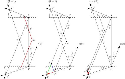
We first observe that if and are connected using the trapezoidal map, then both tangent sample points and were added by construction. Clearly, . Therefore, we consider the scenario when and are not connected using the trapezoidal map. Without loss of generality, let lie on the -axis with , and let lie between and .
If both and lie on the same side of the line through , we assume that without loss of generality, they lie on the left side (see Figure 9). Let be the closest sample point of , and let be the closest sample point of , such that and . Observe that must be above , and similarly, must be below .
Since is the closest sample point to and is the closest sample point of , we have that and . If overlaps no obstacles, . Since we do not need to take a detour from to , it is sufficient to find an upperbound on . Therefore, we focus on the worse case where overlaps at least one obstacle. Let be the intersection of and . It remains true that if an obstacle overlaps and simultaneously, there must exist a propagated sample point on that is closer to than is. Therefore the arguments in Lemma 4.8 apply, and .
Let be the intersection of and (see Figure 10, left). We argue that is maximised when lies on and lies on . Then, when both and lie on their respective rays, we show that the total length is at most . To do this, we partition the latter and show that each partition (or two partitions combined) pays for a segment in the former.
By constructing the sample points, and must reside in . The segment must lie between the directions and , as otherwise, and are connected via the trapezoidal map. As a result, , and is to the right of . See Figure 10, right for the following definitions. Let be the intersection of and . Observe that and . Let (resp. ) be the intersection of (resp. ) and . Both and are well-defined, since , , and are parallel. The points and are defined similarly.
Using the triangle inequality, we have that . We observe that and . Combining the above facts, if we focus on , we have
| (1) |
Similarly,
| (2) |
Combining (1) and (2), and the fact that , we have the following.

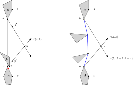
Using analogous arguments, if and lie on the opposite sides of (see Figure 11, left), and an obstacle overlaps , part of must lie in either triangle or (not both).
Without loss of generality, assume that overlaps . If additionally overlaps , a propagated sample point is closer to than , contradicting the assumption that is the closest sample point. An analogous argument applies when overlaps . Therefore if overlaps , then must reside in the either or , where (resp. ) is the intersection of (resp. ) and .
We can construct two convex paths and (see Figure 11, right); resides in and connects to , and resides in and connects to . By Lemma 4.3, we have that
| (1) |
We now upperbound (1). Let be the intersection of and (see Figure 12). Let point be the reflection of along . Observe that since is above , must be above , and . Let (resp. ) be the intersection of (resp. .
Using an analogous charging argument, we have that
Combining with the bound on in the case that and lie on the same side of , we have that
4.3.3 Case 3: connects a 0-region and an obstacle
In this section, we prove that if connects an obstacle and a -region , there is a path that approximate .
Lemma 4.13.
Let be a convex obstacle and let be a convex -region. Let , where and . There exists a pair of sample points and , such that .
Proof 4.14.

Let be aligned with the -axis, such that . If is in some direction , then both and are sample points, and . Therefore, we consider the case where is between direction and . Let (resp. ) be the acute angle between (resp. ) and (see Figure 13).
Let be the first sample point in a counter-clockwise order after . Let be the first sample point in a clockwise order after . Let be the intersection of and . By convexity and the placement of our sample points, must be above , and must lie below .
If is parallel with , then cannot overlap any obstacle . Otherwise, there exists a sample point in the direction of (see Figure 13, left). Since must lie on or to the left of , generates a propagated sample point on , and is closer to than is, contradicting the assumption that is the closest sample point. Therefore, .
To bound , we observe that is maximised when lies on (see Figure 13, right). Let be the intersection of and . Observe that is perpendicular to . We have that , since is a leg of the right triangle , and is the hypotenuse. Using the arguments in Lemma 4.10, . We thus have a path from to via and of length
If is not parallel with , the ray must intersect at some point ( does not propagate to ). For the same reasons as before, an obstacle overlaps neither nor . Let . Consider sliding towards along the concatenated polygonal chain until the ray touches (see Figure 14). Observe that cannot intersect an obstacle during the slide. Indeed, if touches an obstacle at point , must be a sample point with respect to the direction , and propagates to with the ray . Let (resp. ) be the point on such that (resp. ) is parallel to . Let be the intersection of and . Let be the point on such that is parallel to .
When we stop the sliding, either 1) is on , or 2) is on (see Figure 14, left and middle, respectively). In order to avoid obstacles, we have to take a detour from to . In both cases, we argue that the length of the detour is at most . In case 1, the maximum length of the detour we must take is . We use a charging argument: pays for , and pays for . , and by triangle inequality, . Therefore, .
In case 2, the maximum length of the detour is . Let be the point on such that is parallel to . Let be the intersection of and . Let be the point on such that is parallel to . Using analogous argument, pays for , and pays for . By triangle inequality, pays for , and pays for . For both cases, we have that
| (1) |
Next, we argue that is at most (see Figure 14, right). Let be the point on such that is parallel to . By construction, is parallel to , and is parallel to . The triangle is therefore a right triangle with as the hypotenuse. , and therefore we have that
| (2) |
Combining (1), (2), Lemma 2.2, and the fact that lies in a 0-region, we complete the proof with the following.
4.4 The quality of the path
In Lemma 4.10, 4.11, and 4.13, we have shown that for every segment in Case 1-3 in Fact 2, either there exists a path such that approximates , or there exist two sample points and such that approximates . Taking the maximum ratio in the three lemmas, we have the following.
For a Case 4 segment , where both and lies on the obstacle , assume without loss of generality that occurs before in , and let .
If contains no sample point, then assume that the optimal path uses segment to reach , and to leave . We argue that there exists an approximate path that approximates . Let (resp. ) be the closest sample point to (resp. ), such that . In Lemma 4.10, 4.11, and 4.13, we have payed for a path from to though and a path from to through . Since there is no sample point on , instead of going from to and to , we take the path directly. The unused cost of and pays for .
Let (resp. ) be the orthogonal projection of (resp. ) on . Clearly, and . By Lemma 4.3, . Therefore, we connect and using to generate a path , and we have that
If contains at least one sample point , then by Lemma 4.3, we have that
Bose and van Renssen [6] showed that in an environment with polygonal obstacles, a -graph has a spanning ratio of at most . We also need to apply the factor to traverse the boundaries of convex obstacles to account for the difference compared to the boundaries of simplified obstacles, as in Lemma 4.3. We obtain the following bound when .
Given an approximation error , we compute the parameter as the following.
Lemma 4.15.
In , there exists a path between any pair of sample points such that .
4.5 Finding a shortest path amidst -regions and obstacles
Given the data structure , a point , and a point , we query the approximate shortest path from to using Algorithm 4.
This algorithm takes as input a data structure storing a set of 0-regions and a set of obstacles, a point , and a point . It outputs an -approximated weighted shortest path from to . In Step 2 and Step 3, this algorithm shows how to add to , and the same operations are used to add .
-
1.
Add and to .
-
2.
For each trapezoidal map , do the following for point .
-
(a)
Query the face containing . Let be adjacent to and , .
-
(b)
Add the propagated sample points and —which are generated by and , respectively—to .
-
(c)
If is a -region, add and set . Do the same for .
-
(d)
If is an obstacle, add , and set . Compute the common tangents of and . For each common tangent touching at point , add to . Do the same for .
-
(a)
-
3.
Add and the additional sample points generated in Step 2 to . For each newly added point , using as the apex, we construct a set of disjoint cones with angle . For each point closest to in each cone, add to , and set . For every existing vertex , and every existing edge . If is closer to than is, add to , and set .
-
4.
Use Dijkstra’s shortest path algorithm to compute a path from to in . Transform into a path in the original environment and return .
Using the query algorithm, we treat both and as convex obstacles with no interior. This preserves the properties of the trapezoidal maps and the -graph, and enables us to apply the earlier lemmas.
4.5.1 Analysis
We now analyse the query time. In Step 2, we perform a set of operations for each of the trapezoidal maps. In Step 2a, it takes time to find the face containing . In Step 2b, it takes time to use a binary search to compute the intersection of a ray and a convex boundary with complexity. In Step 2c, it takes time to compute the distance between and a convex region using the algorithm by Edelsrunner [15]. In Step 2d, it takes time to compute the common tangent using the algorithms by Kirkpatrick and Snoeink [19], and Guibas et al. [18]. In total, Step 2 takes time.
Inserting into generates a constant number of sample points. In Step 3, for each additional sample point , it takes time to find the closest point of in each cone, and at the same time, check if is closest to any point . In Step 4, it takes to run Dijkstra’s shortest path algorithm. There are vertices, and edges, therefore Dijkstra’s algorithm takes time to return a path comprised of at most edges. It takes time to transform into a path in the environment by traversing the boundaries of the regions.
In total, it takes time to query the approximate - shortest path. Combining the above analysis with Lemma 4.2, 4.10, 4.11, and 4.13, we have the following.
See 1.3
References
- [1] Lyudmil Aleksandrov, Anil Maheshwari, and Jörg-Rüdiger Sack. Approximation algorithms for geometric shortest path problems. In Proceedings of the Thirty-second Annual ACM Symposium on Theory of Computing, pages 286–295, New York, NY, USA, May 2000. Association for Computing Machinery.
- [2] Lyudmil Aleksandrov, Anil Maheshwari, and Jörg-Rüdiger Sack. Determining approximate shortest paths on weighted polyhedral surfaces. Journal of the ACM, 52(1):25–53, January 2005.
- [3] Helmut Alt and Michael Godau. Computing the Fréchet distance between two polygonal curves. International Journal of Computational Geometry & Applications, 05:75–91, March 1995.
- [4] Prosenjit Bose, Jean-Lou de Carufel, Pat Morin, André van Renssen, and Sander Verdonschot. Towards tight bounds on theta-graphs: More is not always better. Theoretical Computer Science, 616:70–93, February 2016.
- [5] Prosenjit Bose, Guillermo Esteban, David Orden, and Rodrigo I. Silveira. On approximating shortest paths in weighted triangular tessellations. Artificial Intelligence, 318:103898, May 2023.
- [6] Prosenjit Bose and André van Renssen. Spanning properties of Yao and theta-graphs in the presence of constraints. International Journal of Computational Geometry & Applications, 29(02):95–120, June 2019.
- [7] Kevin Buchin, Maike Buchin, and Yusu Wang. Exact algorithms for partial curve matching via the Fréchet distance. In Proceedings of the Twentieth Annual ACM-SIAM Symposium on Discrete Algorithms, pages 645–654, USA, January 2009. Society for Industrial and Applied Mathematics.
- [8] Kevin Buchin, Tim Ophelders, and Bettina Speckmann. SETH says: weak fréchet distance is faster, but only if it is continuous and in one dimension. In Proceedings of the Thirtieth Annual ACM-SIAM Symposium on Discrete Algorithms, pages 2887–2901, USA, January 2019. Society for Industrial and Applied Mathematics.
- [9] Siu-Wing Cheng, Jiongxin Jin, and Antoine Vigneron. Triangulation Refinement and Approximate Shortest Paths in Weighted Regions. In Proceedings of the 2015 Annual ACM-SIAM Symposium on Discrete Algorithms, Proceedings, pages 1626–1640. Society for Industrial and Applied Mathematics, December 2014.
- [10] Kenneth L. Clarkson. Approximation algorithms for shortest path motion planning. In Proceedings of the nineteenth annual ACM Symposium on Theory of Computing, pages 56–65, New York, NY, USA, January 1987. Association for Computing Machinery.
- [11] Mark de Berg, Otfried Cheong, Marc van Kreveld, and Mark Overmars. Computational Geometry: Algorithms and Applications. Springer, Berlin, Heidelberg, 2008.
- [12] Sarita de Berg, Guillermo Esteban, Rodrigo I. Silveira, and Frank Staals. Exact solutions to the Weighted Region Problem, February 2024. arXiv:2402.12028 [cs].
- [13] Jean-Lou de Carufel, Amin Gheibi, Anil Maheshwari, Jörg-Rüdiger Sack, and Christian Scheffer. Similarity of polygonal curves in the presence of outliers. Computational Geometry, 47(5):625–641, July 2014.
- [14] Jean-Lou de Carufel, Carsten Grimm, Anil Maheshwari, Megan Owen, and Michiel Smid. A note on the unsolvability of the weighted region shortest path problem. Computational Geometry, 47(7):724–727, August 2014.
- [15] Herbert Edelsbrunner. Computing the extreme distances between two convex polygons. Journal of Algorithms, 6(2):213–224, June 1985.
- [16] Jeff Erickson. Algorithms. First edition, June 2019.
- [17] Laxmi P. Gewali, Alex C. Meng, Joseph S. B. Mitchell, and Simeon Ntafos. Path planning in 0/1/infinity weighted regions with applications. In Proceedings of the Fourth Annual Symposium on Computational Geometry, pages 266–278, New York, NY, USA, January 1988. Association for Computing Machinery.
- [18] Leonidas Guibas, John Hershberger, and Jack Snoeyink. Compact interval trees: a data structure for convex hulls. International Journal of Computational Geometry & Applications, 01(01):1–22, March 1991.
- [19] David Kirkpatrick and Jack Snoeyink. Computing common tangents without a separating line. In Gerhard Goos, Juris Hartmanis, Jan Leeuwen, Selim G. Akl, Frank Dehne, Jörg-Rüdiger Sack, and Nicola Santoro, editors, Algorithms and Data Structures, volume 955, pages 183–193. Springer Berlin Heidelberg, Berlin, Heidelberg, 1995. Series Title: Lecture Notes in Computer Science.
- [20] Mark Lanthier, Anil Maheshwari, and Jörg-Rüdiger Sack. Approximating weighted shortest paths on polyhedral surfaces. In Proceedings of the Thirteenth Annual Symposium on Computational Geometry, pages 274–283, New York, NY, USA, August 1997. Association for Computing Machinery.
- [21] Joseph S. B. Mitchell and Christos H. Papadimitriou. The weighted region problem: finding shortest paths through a weighted planar subdivision. Journal of the ACM, 38(1):18–73, January 1991.
- [22] Giri Narasimhan and Michiel Smid. Geometric Spanner Network. Cambridge University Press, 2007.
- [23] Zheng Sun and John H. Reif. On finding approximate optimal paths in weighted regions. Journal of Algorithms, 58(1):1–32, January 2006.
- [24] Victor Andreevich Toponogov. Differential Geometry of Curves and Surfaces: A Concise Guide. Birkhauser.