Description of Molecular Chirality and its Analysis via High Harmonic Generation

Abstract

To clarify the microscopic origin of chirality-induced optical effect, we develop an analytical method that extracts the chiral part of the Hamiltonian of molecular electronic states. We demonstrate this method in a model chiral molecule consisting of helically stacked two $N$ regular polygons, and compare it with numerical calculation for chiral discrimination via high-harmonic generation (HHG) of the same molecule. The discrimination signal here is the difference between the harmonic intensity from the bicircular laser field and that from its reflected laser field, resulting in a pseudoscalar quantity that reflects the chirality of the molecule. As a result, we find that, to obtain the large discrimination signal via HHG difference, the increase of capacity to generate the polar quantity is more advantageous than maximizing the conversion efficiency via the optimization of molecular chirality. We speculate this criteria may be extended to other optical and current-induced processes relevant to the chiral molecules and materials.

I Introduction

Chirality, a structural property of an object that lacks reflection and inversion symmetries, is ubiquitous in nature from single molecules, molecular assemblies, crystals to living organisms  [1]. Much effort has been devoted toward understanding the functionality inherent in the chiral systems. In crystals, electronic and phononic band splittings are originated from the chiral symmetry breaking  [2, 3, 4, 5, 6, 7, 8], which has invigorated possibilities in transporting and converting their angular momentums (AMs)  [9, 10, 11]. In particular, properties of the AM in the chiral systems and its relevance to chirality-induced spin selectivity (CISS)  [12, 13, 14, 15] effect have been increasingly focused on. Thus, as well as elucidating the characteristics of chiral materials and establishing efficient means of asymmetric synthesis, discriminating the chirality is also the indispensable problem.

Recent studies have demonstrated that the chirality in quantum systems can be represented as the electric toroidal monopole (ETM)  [16, 17, 18, 19]. This is anti-symmetric with respect to the inversion and reflection and has the time-reversal symmetry, and thus is a generalization of the definition of the chirality by Kelvin and Barron [20]. Because also Hamiltonian of chiral systems should include the ETM, we can formally separate it into the symmetric and anti-symmetric part. The anti-symmetric part is defined by the subtraction of the Hamiltonians with the opposite chiralities, which belongs to the different Hilbert spaces composed of the different electronic basis set. Then, its direct evaluation has a major difficulty. One of the main results of this work is that we develop a method to enables the direct subtraction of the matrix elements, and thus the identification of the chirality.

Using the above identification method, we consider the chiral discrimination signal by light as one example. The chiral systems asymmetrically interact with the chiral light, which can be utilized to optically discriminate the chirality. In circular dichroism (CD), the differential absorption spectrum between the clockwise and the counterclockwise circular polarization of light, which correspond to the spin angular momentum (SAM), is measured. The measured spectrum is the pseudoscalar quantity, i.e., each enantiomer has the opposite sign from the other. The ability to extract the pseudoscalar (more generally the pseudotensor) spectrum can be a clear manifestation of the chiral discrimination. Therefore, it is natural to explore criteria from a microscopic point of view on how to extract a large pseudoscalar spectrum.

Here, we focus on a nonlinear optical process called high harmonic generation (HHG), which is the light emission with frequencies multiple integers of the injected one. As a consequence of the SAM conservation, the atoms and molecules cannot emit the high-harmonics from the light beams with the single circular polarization and requires the bicircular field, the combination of both circular polarizing fields [21, 22, 23]. This bicircular field can break the reflection symmetry, and thus, can be chiral. Therefore, the chiral discriminating HHGs using the bicircular field have been studied [24, 25, 26, 27, 28, 29], wherein the HHG spectrum measurements have demonstrated that its Kuhn $g$-factor is pseudoscalar. We demonstrate our developed identification method in a model chiral molecule consisting of helically stacked two $N$ regular polygons, and compare it with numerical calculation within so-called three-step model [30, 31]. It is found that the increase of the polar quantity is more advantageous than maximizing the conversion efficiency of the molecular chirality to obtain the large difference between the harmonic intensity from the bicircular laser field and that from its reflected laser field.

The remaining part of this paper is organized as follows: In Section II, we introduce the model chiral molecule and its the anti-symmetric part is deduced in Section III. In Section IV, we present the theory of the HHG basisd on the three step model and prove that the Kuhn $g$-factor becomes pseudoscalar using the symmetry argument. In Section V, numerical results of the chiral discriminating HHGs are presented and its correspondence to the chiral part of the Hamiltonian are analyzed. Section VI is devoted to the concluding remarks.

II Model Chiral Molecule

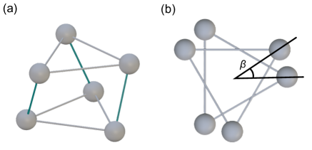
Figure 1: (a) Illustration of the model chiral molecule that consists of two $N=3$ regular polygons. The grey and green lines display the intralayer and interlayer bonds. (b) Top view of our model. Regular polygons are helically stacked with the twist angle $\beta$.

As a model chiral system, we consider a helical stacking of two $N$ regular polygon molecules (see Fig. 1 for $N=3$) characterized by the radius $\rho$, the interlayer distance $h$, and the twist angle $\beta$. The position of the $j$th atom ($j=1,\ldots,N$) in the $k$th layer ($k=1,2$) is written as $\bm{R}_{kj}(\beta)=(\rho\cos 2\theta_{kj},\rho\sin 2\theta_{kj},(k-1)h)^{\top}$ with $\theta_{kj}=(k-1)\beta/2+(j-1)\alpha/2$ and $\alpha=2\pi/N$ being the rotation angle. To break the reflection symmetry, the twist angle have to satisfy $0<\vab{\beta}<\alpha/2$. Chirality reversal corresponds to the inversion of the twist angle, $\beta\to-\beta$, under the action of the reflection operator $\hat{\sigma}$ with respect to the $xz$-plane, $\hat{\sigma}\bm{R}_{kj}(\beta)=\bm{R}_{kj}(-\beta)$.

Based on the Slater–Koster method [32, 33], we construct the tight-binding Hamiltonian $\hat{H}(\beta)$ using the electronic basis states $\{\ket*{\phi_{kj}^{\nu}(\beta)}\}$ that consist of $2\mathrm{s}$ ($\nu=0$) , $2\mathrm{p}_{z}$ ($\nu=z$), and $2\mathrm{p}_{\pm}=2\mathrm{p}_{x}\pm i2\mathrm{p}_{y}$ ($\nu=\pm$) orbitals from each atom, where $\ket*{\phi_{kj}^{\nu}(\beta)}$ represents the orbital $\nu$ centered at $\bm{R}_{kj}(\beta)$, $\innerproduct*{\bm{r}}{\phi_{kj}^{\nu}(\beta)}=\phi^{\nu}(\bm{r}-\bm{R}_{kj}(\beta))$. We consider the electronic bonds between the adjacent atoms in the same layer (intralayer) and the ones with the same $j$ in the different layers (interlayer). The latter bond is characterized by the helical angle $\gamma=\arctan(h/2\rho\sin(\beta/2))$ and is necessary to endow the chirality with the electronic state. The Slater–Koster overlaps for the intralayer bond are denoted by $V_{\lambda\nu}^{s}$ ($s=\sigma$ and $\pi$ for parallel with and perpendicular to the bonding), which is parametrized by $V$, and those for the interlayer bond are denoted by $W_{\lambda\nu}^{s}$, which is parametrized by $W$. For the constructed Hamiltonian and its detailed derivation, see Appendix. A.

The groundstate $\ket{\phi_{\mathrm{GS}}(\beta)}$ is the eigenstate of $\hat{H}(\beta)$, and hence, belong to the irreducible representation (IRREP) of the point group $\mathrm{C}_{N}$, because $\hat{H}(\beta)$ possess the $N$-fold rotational symmetry. Each eigenstate $\ket*{\phi_{m}(\beta)}$ is classified by its rotational quantum number or the pseudo AM [9, 34], $m$, through the relation $\hat{C}_{N}\ket{\phi_{m}(\beta)}=e^{-im\alpha}\ket{\phi_{m}(\beta)}$ with $\hat{C}_{N}$ being the $N$-fold rotational operator. For $N$-odd and even cases, the pseudo AM takes the value $m=0,\pm 1,\ldots,\pm(N-1)/2$ and $m=0,\pm 1,\ldots,\pm(N-1)/2,N/2$, respectively. The time-reversal symmetry enforces the degeneracy of $\ket*{\phi_{m}(\beta)}$ and $\ket*{\phi_{-m}(\beta)}$. Thus, the groundstate becomes $\ket{\phi_{\mathrm{GS}}(\beta)}=(\ket*{\phi_{m}(\beta)}+\ket*{\phi_{-m}(\beta)})/\sqrt{2}$.

III Description of Molecular Chirality

To discuss the correspondence between the molecular chirality and the Kuhn $g$-factor, we extract the anti-symmetric part of the Hamiltonian with respect to the reflection operation. This part is formally written as $\hat{G}_{0}(\beta)=[\hat{H}(\beta)-\hat{H}(-\beta)]/2$, which satisfies $\hat{\sigma}\hat{G}_{0}(\beta)\hat{\sigma}^{\dagger}=-\hat{G}_{0}(\beta)$. Because the matrix element $\innerproduct*{[}{[}3]{\phi_{ki}^{\lambda}(\beta^{\prime})}{\hat{H}(\beta)}{\phi_{lj}^{\nu}(\beta^{\prime})}$ is well-defined only for the $\beta=\beta^{\prime}$ cases, the direct subtraction of the Hamiltonians with the opposite $\beta$ requires the transformation from $\ket*{\phi_{kj}^{\nu}(0)}$ to $\ket*{\phi_{kj}^{\nu}(\pm\beta)}$. For that purpose, we first translate the orbital center from $\bm{R}_{kj}(\beta)$ to $\bm{R}_{kj}(0)$ as

$$\phi^{\nu}(\bm{r}-\bm{R}_{kj}(0)) =\exp\ab[-\frac{i}{\hbar}\bm{\hat{p}}\cdot(\bm{R}_{kj}(0)-\bm{R}_{kj}(\beta))]$$

$$\quad\times\phi^{\nu}(\bm{r}-\bm{R}_{kj}(\beta))$$

$$=\hat{T}_{kj}(\beta)\phi^{\nu}(\bm{r}-\bm{R}_{kj}(\beta)),$$ (1)

where $\hat{\bm{p}}=-i\hbar\bm{\nabla}$ is the momentum operator. This procedure is similar to pullback or push forward mapping in the Lie derivative [35]. Expressing the orbital as the product of the radial distribution and the spherical harmonics, the achiral basis with $\beta=0$ can be written as a linear combination of the chiral basis states,

$$\ket*{\phi_{kj}^{\nu}(0)}=\hat{T}_{kj}(\beta)\ket*{\phi_{kj}^{\nu}(\beta)}=\sum_{\nu^{\prime}}g_{kj}^{\nu\nu^{\prime}}(\beta)\ket*{\phi_{kj}^{\nu^{\prime}}(\beta)}$$ (2)

with $g_{kj}^{\nu\nu^{\prime}}(\beta)\in\mathbb{C}$ (see Appendix. B for details). This allows us to expand the Hamiltonians with the achiral basis states as $\hat{H}(\beta)=\sum_{klij\lambda\nu}\innerproduct*{[}{[}3]{\phi_{ki}^{\lambda}(0)}{\hat{H}(\beta)}{\phi_{lj}^{\nu}(0)}\outerproduct*{\phi_{ki}^{\lambda}(0)}{\phi_{lj}^{\nu}(0)}$ with

$$\innerproduct*{[}{[}3]{\phi_{ki}^{\lambda}(0)}{\hat{H}(\beta)}{\phi_{lj}^{\nu}(0)}$$

$$=\sum_{\lambda^{\prime}\nu^{\prime}}(g_{ki}^{\lambda\lambda^{\prime}}(\beta))^{\ast}g_{lj}^{\nu\nu^{\prime}}(\beta)\innerproduct*{[}{[}3]{\phi_{ki}^{\lambda^{\prime}}(\beta)}{\hat{H}(\beta)}{\phi_{lj}^{\nu^{\prime}}(\beta)},$$ (3)

This procedure also applies to $\hat{H}(-\beta)$, and hence, allows us to directly evaluate the anti-symmetric term $\hat{G}_{0}(\beta)$ by simply subtracting the matrix elements. For the small $\beta$, $\hat{G}_{0}(\beta)$ is decomposed into two terms as

$$\hat{G}_{0}(\beta)=\hat{G}_{0}^{\mathrm{coup}}(\beta)+\hat{G}_{0}^{\mathrm{pos}}(\beta)+\mathcal{O}(\beta^{2}),$$ (4)

where $\hat{G}_{0}^{\mathrm{coup}}(\beta)$ depends on $\beta$ from the interlayer bonds described by the helical angle $\gamma$ and $\hat{G}_{0}^{\mathrm{pos}}(\beta)$ depends on $\beta$ from the atomic position itself combined with the $\gamma$-independent interlayer coupling elements. The former is expressed as

$$\innerproduct*{[}{[}3]{\phi_{2j}^{\lambda}(0)}{\hat{G}_{0}^{\mathrm{coup}}(\beta)}{\phi_{1j}^{\nu}(0)}=\frac{i}{\sqrt{2}}\frac{\rho\beta}{h}\begin{pmatrix}O&M\\ -M^{\dagger}&O\end{pmatrix},$$ (5)

where $\nu$ is taken in order $\{0,z,+,-\}$. The $2\times 2$ matrix $M$ is defined by $M_{11}=-M_{12}=W_{sp}^{\sigma}$ and $M_{21}=-M_{22}=W_{pp}^{\sigma}-W_{pp}^{\pi}$. Thus, the chirality appears as the imaginary hopping, which is proportional to the radius $\rho$ and inversely to the interlayer distance $h$. This feature is consistent with the fact that $\rho/h$ corresponds to the ratio between the curvature and the torsion in helices. The latter is expressed as

$$\innerproduct*{[}{[}3]{\phi_{2j}^{\lambda}(0)}{\hat{G}_{0}^{\mathrm{pos}}(\beta)}{\phi_{1j}^{\nu}(0)}=\frac{\zeta\rho\beta}{\sqrt{2}}\begin{pmatrix}0&0&u_{1}&u_{1}^{\ast}\\ 0&0&-u_{1}&-u_{1}^{\ast}\\ -u_{2}^{\ast}&0&0&0\\ u_{2}&0&0&0\end{pmatrix},$$ (6)

with $u_{1}=-ie^{-i(j-1)\alpha}W_{ss}^{\sigma}/\sqrt{3}$, $u_{2}=\sqrt{3}e^{-i(j-1)\alpha}W_{pp}^{\pi}/2$, and $\zeta$ being the exponent of the radial component of the orbitals. Hereafter, we compare this result with the numerical calculation results in Sec. V.

IV Chiral Discriminating High-Harmonic Generation

IV.1 Three step model

Typical spectra and behaviors of HHG for molecular systems can be successfully explained by the three-step model [30, 31]: The electron is first tunnel-ionized, which is further accelerated by the laser field. Finally, the electron recombines with its parent ion emitting the high-harmonics. The intensity of the $n$th harmonics is given by $I_{n}=(n\omega)^{4}\vab*{\bm{\mu}(n\omega)}^{2}=(n\omega)^{4}\vab*{\int_{0}^{\infty}\difc{t}{}\,\bm{\mu}(t)e^{in\omega t}}^{2}$ with $\bm{\mu}$ being the electric dipole moment. In the quantum mechanical formulation of the three step model, the electron–photon interaction is treated within the electric dipole approximation. Furthermore, assuming that only the single active electron participates in the HHG process, the depletion of the ground state can be neglected, and the nuclear positions are fixed (the frozen nuclear approximation), the electric dipole moment at time $t$ is represented as  [31, 36, 37]

$$\bm{\mu}(t) =\imaginary\int_{0}^{t}\difc{\tau}{}\,C(\tau)\bm{d}^{\ast}(\bm{p}_{\mathrm{st}}-e\bm{A}(t))e^{-\frac{i}{\hbar}S(\bm{p}_{\mathrm{st}},t,t-\tau)}$$

$$\times\bm{d}(\bm{p}_{\mathrm{st}}-e\bm{A}(t-\tau))\cdot\bm{E}(t-\tau),$$ (7)

with $C(\tau)=\frac{2}{\hbar}\ab(\frac{2\pi m_{\mathrm{e}}\hbar}{\eta+i\tau})^{3/2}$, the vector potential $\bm{A}$, the electric field $\bm{E}=-\difcp{\bm{A}}{t}$, the electron charge $e$, and the electron mass $m_{\mathrm{e}}$. Here, $\eta$ and $\bm{p}_{\mathrm{st}}=\int_{t-\tau}^{t}\difc{t^{\prime}}{}\,e\bm{A}(t^{\prime})/\tau$ denote the regularization constant and the stationary momentum, respectively, both of which come from the saddle point approximation in the momentum space integral. During the acceleration process, the strong field approximation is invoked, wherein the interaction between the ionized electron and the nuclei is neglected, yielding the propagator described by the action $S(\bm{p},t,t-\tau)=\int_{t-\tau}^{t}\difc{t^{\prime}}{}[(\bm{p}-e\bm{A}(t^{\prime}))^{2}/2m_{\mathrm{e}}+I_{\mathrm{p}}]$ with $I_{\mathrm{p}}$ being the ionization potential. The ionization amplitude is defined as $\bm{d}(\bm{p})=\innerproduct*{[}{[}3]{\bm{p}}{e\hat{\bm{r}}}{\phi_{\mathrm{GS}}}$, where $\hat{\bm{r}}$ is the electron position operator. In this formulation, the chiral effect is contained in $\bm{d}$ and $\bm{d}^{\ast}$ through the dependence on $\ket{\phi_{\mathrm{GS}}(\beta)}$. In our model, where the groundstate is given by $\ket*{\phi_{\mathrm{GS}}(\beta)}=(\ket*{\phi_{m}(\beta)}+\ket*{\phi_{-m}(\beta)})/\sqrt{2}$, $\bm{\mu}(t)$ is a sum of the IRREP-resolved electric dipoles, $\bm{\mu}(t)=[\bm{\mu}_{m}(t)+\bm{\mu}_{-m}(t)]/2$, where $\bm{\mu}_{m}(t)$ is obtained by replacing $\ket{\phi_{\mathrm{GS}}(\beta)}$ in Eq. (7) with $\ket*{\phi_{m}(\beta)}$, because the ionized electron returns to its original state or orbital, and hence, the mixing of the states with the different $m$ can be neglected.

IV.2 Pseudoscalar property of HHG signal

The chiral discrimination is quantified by the Kuhn $g$-factor [38], which is generalized to the HHG signals as defined below. To prove that the Kuhn $g$-factor is a pseudoscalar quantity, we assume that the molecular rotational axis is fixed and parallel with the propagation direction of the light beams. This assumption affects the signals quantitatively, but is not the prerequisite for the pseudoscalar nature as exemplified by the numerical [28] and experimental [24, 25] studies for randomly oriented molecules. Then, the vector potential for the bicircular field is given by

$$\bm{A}(t)=A_{+}\bm{e}_{+}e^{-ir_{+}\omega t}+A_{-}\bm{e}_{-}e^{-ir_{-}\omega t}+\mathrm{c.c.},$$ (8)

where $\bm{e}_{\pm}=\frac{1}{\sqrt{2}}(1,\pm i,0)^{\top}$ are the polarization vectors and $A_{\pm}$ is the corresponding amplitudes with the fundamental frequency $\omega$ and $r_{\pm}\in\mathbb{N}$. This is transformed under the reflection operation to $\bar{\bm{A}}(t)=\hat{\sigma}\bm{A}(t)$ obtained by interchanging the polarization vectors, $\bm{e}_{\pm}\to\bm{e}_{\mp}$. In the cases of $A_{+}\neq A_{-}$ or $r_{+}\neq r_{-}$, the inequality $\bar{\bm{A}}(t)\neq\bm{A}(t)$ holds, and thus, the bicircular field is chiral. The reflection operation also acts as $\hat{\sigma}\ket*{\phi_{m}(\beta)}\equiv\ket*{\phi_{-m}(-\beta)}$, which straghtforwardly leads to $\bm{\mu}(n\omega,\bm{A},\beta)=\hat{\sigma}\bm{\mu}(n\omega,\bar{\bm{A}},-\beta)$, and thus, $I_{n}(\bm{A},\beta)=I_{n}(\bar{\bm{A}},-\beta)$. Now, it is clear that the Kuhn $g$-factor

$$g(\beta)\coloneqq 2\frac{I_{n}(\bm{A},\beta)-I_{n}(\bar{\bm{A}},\beta)}{I_{n}(\bm{A},\beta)+I_{n}(\bar{\bm{A}},\beta)},$$ (9)

is pseudoscalar, $g(\beta)=-g(-\beta)$, for all harmonic orders $n$. We also introduce the unnormalized $g$-factor, which we call $\tilde{g}$-factor, as $\tilde{g}(\beta)\coloneqq I_{n}(\bm{A},\beta)-I_{n}(\bar{\bm{A}},\beta)$ to discuss the correspondence between the molecular chirality and the HHG signal. The $\tilde{g}$-factor is also the pseudoscalar.

V Results

To calculate the electric dipole moment Eq. (7), we performed the numerical integration using the Gauss–Kronrod quadrature method [39] with the quad precision arithmetics. Throughout the calculation, we set to $\omega A_{+}=\quantity[per-mode=symbol]{3d10}{\per}$, $\omega A_{-}=\quantity[per-mode=symbol]{4d10}{\per}$, $r_{+}=1$, $r_{-}=2$, and $\omega=\quantity{1}{}$ for the laser field, and $\rho=\quantity{0.256}{}$, $V=\quantity{0.5}{}$, $W=\quantity{0.2}{}$, and $I_{\mathrm{p}}=\quantity{14}{}$ for the chiral molecule. Hereafter, we focus on the $N=3$ with $m=\pm 1$ case only, but the qualitative consistency was also checked for the $N=4$ with $m=\pm 1$ and the $N=6$ with $m=\pm 1$ and $\pm 2$ cases.

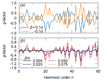
Figure 2: (a) Calculated $g$-factors for $\beta=0.1\,\alpha$ (blue line) and $\beta=-0.1\,\alpha$ (orange line). Each enantiomer is interconverted to the other by inverting $\beta$. (b) Twist angle, $\beta$, dependence of the $g$-factor. The interlayer distance is fixed to $h=\quantity{0.6}{}$.

Figure 3: (a) Calculated $\tilde{g}$-factors for various values of the interlayer distance, $h$. (b) The $\tilde{g}$-factor decomposition into the $x+y$-component, $\vab*{\mu_{x}(n\omega)}^{2}+\vab*{\mu_{y}(n\omega)}^{2}$, and the $z$-component, $\vab*{\mu_{z}(n\omega)}^{2}$, for the harmonic orders $n=28$ and $34$. Twist angle is fixed to $\beta=0.005\,\alpha$.

Figure 2(a) depicts the $g$-factor for each enantiomer of our model chiral molecule. The pseudoscalar property is confirmed for all harmonic orders $n$, because the $g$-factor is reversed by inverting the twist angle, $\beta$. The $g$-factor has a value in $-2\leq g\leq 2$ and its increasing is advantageous for the chiral discrimination. In Fig. 2(a), this value can exceeds $1.0$, which is much larger than typical values of the CD. This is because the CD is contributed from the magnetic dipole moment in the light–matter interaction, the magnitude of which is sufficiently smaller than that of the electric dipole moment.

Next, we examine the correspondence between the molecular chirality of Eqs. (5), (6) and the $g$-factor. Hereafter, we focus on the small $\beta$ region, where the Hamiltonian is approximated as $\hat{H}(\beta)\approx\hat{H}(0)+\hat{G}_{0}^{\mathrm{coup}}(\beta)+\hat{G}_{0}^{\mathrm{pos}}(\beta)$. In Fig. 2(b), we present the $g$-factors for the various values of $\beta$, where the $g$-factor monotonically increases as $\beta$ is increased. Because the twist angle does not change the molecular size, which is the another element to affect the signal, this feature can be attributed to the linear $\beta$-dependence of $\hat{G}_{0}^{\mathrm{coup}}(\beta)$ and $\hat{G}_{0}^{\mathrm{pos}}(\beta)$, and thus, the increase of the molecualr chirality.

To analyze the correspondance without consideration of the effects from $\hat{G}_{0}^{\mathrm{pos}}(\beta)$, we consider the $h$-dependence of the chiral discriminating signals, because $\hat{G}_{0}^{\mathrm{pos}}(\beta)$ has no $h$-dependence. To remove further the contribution from the symmetric part of the Hamiltonian of the denominator in Eq. (8), we present the $\tilde{g}$-factors for various values of $h$ in Fig. 3(a), where the peak intensities are a monotonic increasing function of $h$. For the peaks of $n=28$ and $34$, we decompose this into $\vab*{\mu_{x}(n\omega)}^{2}+\vab*{\mu_{y}(n\omega)}^{2}$ and $\vab*{\mu_{z}(n\omega)}^{2}$ depicted in Fig. 3(b), where the $x+y$-component is negligibly small, and thus, the $z$-component dominantly contributes to the $\tilde{g}$-factor. We further found that this $z$-component scales quadratically with $h$. To unveil the origin of this, the ionization amplitude $\bm{d}(\bm{p})$ is expanded with the basis states as

$$\bm{d}(\bm{p})=\sum_{kj\nu}b_{kj}^{\nu}e^{-i\bm{p}\cdot\bm{R}_{kj}/\hbar}\ab(\bm{R}_{kj}+i\hbar\difcp*{}{\bm{p}})\tilde{\phi}^{\nu}(\bm{p}),$$ (10)

where $b_{kj}^{\nu}$ is the linear coefficient for the basis $\ket*{\phi_{kj}^{\nu}}$ and $\tilde{\phi}^{\nu}(\bm{p})$ is the momentum representation of $\phi^{\nu}$. Eqs. (7) and (10) shows that the quadratic dependence is originated from the $z$-component, $(\bm{R}_{kj})_{z}=(k-1)h$, of the first term of Eq. (10) for the recombination process, $\bm{d}^{\ast}$, and not the ionization process. This is because the ionization amplitude emerges as the form $\bm{d}\cdot\bm{E}$ and does not depend on this term due to no $z$-component of $\bm{E}(\tau)$. Therefore, the chiral discriminating HHG can be interpreted as the quantification of the longitudinal dipole moment at the recombination converted from the transverse dipole moment in the ionization process. Because increasing the interlayer distance, $h$, decreases $\hat{G}_{0}^{\mathrm{coup}}(\beta)$, simultaneously increasing the molecular size, this result also indicates that the enhancement of the electric dipole moment by enlarging the molecular size contributes dominantly to the $\tilde{g}$-factor rather than increasing the molecular chirality, $\hat{G}_{0}^{\mathrm{coup}}(\beta)$. This may be because the $z$-component of Eq. (10) is proportional to $h$ and unbounded, whereas the chiral contributions from $b_{kj}^{\nu}$ and $\bm{R}_{kj}$ are bounded by the normalization condition of the wavefunction and the helical angle $\gamma$ appeared as $\sin\gamma$ and $\cos\gamma$, respectively. What should be noted here is that this $z$-component is contributed only from the $2\mathrm{p}_{z}$-orbitals, which are involved only in the chiral cases. Indeed, in the achiral case with $\beta=0$, the $2\mathrm{p}_{z}$-orbital belong to the different IRREP from the other orbitals, and thus, they are orthogonal.

VI Concluding Remarks

In this study, we have developed the analytical method that extracts the anti-symmetric part of the Hamiltonian that describes the chirality. Our approach is based on the translation of the orbital center of each electronic basis from the achiral system to the chiral system. This allows us to expand the chiral Hamiltonians with the achiral basis states, enabling the direct subtraction of the matrix elements of the different chirality. As a demonstration of this method, we consider the model chiral molecule that consists of helically stacked two $N$ regular polygons and investigate the correspondence between the chiral part of our model and the Kuhn $g$-factor in HHG. Numerical results shows that the $g$-factor is the pseudoscalar quantity reflecting the chirality of the molecule. Calculated values are much larger than the typical values of the CD and slightly larger than that reported in Ref. [25] of the gaseous molecules. Extension of our result to the randomly oriented molecules may give the quantitatively consistent result with the experiments. Numerical results also reveal that the enhancement of the electric dipole moment dominantly contributes to increasing the spectra even when this enhancement is accompanied by reducing the molecular chirality. This finding may have the following implication: The chiral molecules and materials have an ability to interconvert the polar and axial quantities. This inverconversion works efficiently for the strong chiral systems. However, to obtain the large axial quantity from the polar one, increasing capacity to generate the axial quantity can be effective (and vice versa). We demonstrated this for the light-induced electric dipole moment in the HHG, and therefore, expect that this validity can be extended to other optical processes. Furthermore, this may also be relevant to the effects induced by the metal–molecule interaction with or without the charge injection in the chiral systems, especially the CISS, wherein the interrelation between the charge redistribution and the formation of the anti-parallel spin pair [40, 41, 42] is hypothesized as one of the keys to understand the CISS mechanism [43, 15].

Our method developed in this paper is also applicable to other chiral systems such as helices and crystals. Generalization to the systems with the spin–orbit, electron–phonon, and electron–photon interactions will be of great interest in elucidating the microscopic insight into the AM exchange among them [44, 45, 46], which is left for future studies.

Appendix A Construction of tight-binding Hamiltonian

In this Appendix, the tight-binding Hamiltonian of the model chiral molecule introduced in Sec. II is constructed using the Slater–Koster method following Refs. [32, 33]. For notational simplicity, we omit $\beta$ to specify the chirality from the description.

The matrix element of the Hamiltonian is written as

$$H_{ki,lj}^{\lambda\nu}\coloneqq\innerproduct*{[}{[}3]{\phi_{ki}^{\lambda}}{\hat{H}}{\phi_{lj}^{\nu}}=E_{ki,lj}^{\lambda\nu}\exp\ab(i\xi_{ki,lj}^{\lambda\nu})$$ (11)

where $E_{ki,lj}^{\lambda\nu}$ is the overlap integral and $\xi_{ki,lj}^{\lambda\nu}$ is the phase factor that is determined to maintain the molecular symmetry. Let $\hat{\bm{n}}(\nu_{ki})$ denote the unit vector along the orbital $\ket*{\phi_{ki}^{\nu}}$. Then, the overlap integral can be expressed as

$$E_{ki,lj}^{\lambda\nu} =\aab*{\hat{\bm{n}}(\lambda_{ki}),\hat{\bm{n}}(\nu_{lj})}V_{\lambda\nu}^{\pi}$$

$$+\aab*{\hat{\bm{R}}_{lj,ki},\hat{\bm{n}}(\lambda_{ki})}\aab*{\hat{\bm{R}}_{lj,ki},\hat{\bm{n}}(\nu_{lj})}\ab(V_{\lambda\nu}^{\sigma}-V_{\lambda\nu}^{\pi})$$ (12)

where $V_{\lambda\nu}^{\sigma}$ and $V_{\lambda\nu}^{\pi}$ are the Slater–Koster overlaps and $\bm{R}_{lj,ki}=\bm{R}_{lj}-\bm{R}_{ki}$ is the bond vector. The normalized bond vector, $\hat{\bm{R}}_{lj,ki}\equiv\bm{R}_{lj,ki}/\vab*{\bm{R}_{lj,ki}}$, is given by

$$\hat{\bm{R}}_{lj,ki} =-\sin(\theta_{lj}+\theta_{ki})\cos\gamma_{lj,ki}\bm{e}_{x}$$

$$\quad+\cos(\theta_{lj}+\theta_{ki})\cos\gamma_{lj,ki}\bm{e}_{y}$$

$$\quad+\sin\gamma_{lj,ki}\bm{e}_{z}$$ (13)

with $\theta_{ki}=[(k-1)\beta+(i-1)\alpha]/2$, $\theta_{lj,ki}=\theta_{lj}-\theta_{ki}$ and $\gamma_{lj,ki}=\arctan[(l-k)h/2\rho\sin\theta_{lj,ki}]$. With these notations, $\hat{\bm{n}}(\nu_{ki})$ is written as $\hat{\bm{n}}(s_{ki})=\hat{\bm{R}}_{lj,ki}$, $\hat{\bm{n}}(s_{lj})=-\hat{\bm{R}}_{lj,ki}$, $\hat{\bm{n}}(x_{ki})=\cos 2\theta_{ki}\bm{e}_{x}+\sin 2\theta_{ki}\bm{e}_{y}$, $\hat{\bm{n}}(y_{ki})=-\sin 2\theta_{ki}\bm{e}_{x}+\cos 2\theta_{ki}\bm{e}_{y}$, and $\hat{\bm{n}}(z_{ki})=\bm{e}_{z}$. Hence, we can obtain the analytical expressions of the overlap integrals, $E_{ki,lj}^{\lambda\nu}$, by directly evaluating Eq. (12). The details of the calculation is given in Refs. [33]. Finally, we can obtain the matrix elements for the intralayer bond as

$$H_{kj,kj\pm 1}^{ss} =-V_{ss}^{\sigma}$$ (14)

$$H_{kjkj\pm 1}^{zz} =V_{pp}^{\pi}$$ (15)

$$H_{kj,kj\pm 1}^{zs} =H_{kj,kj\pm 1}^{sz}=0$$ (16)

$$H_{kj,kj\pm 1}^{s\eta} =-H_{kj,kj\pm 1}^{\eta s}=\pm\frac{i\eta}{\sqrt{2}}e^{\pm i\eta\pi/2}V_{sp}^{\sigma}$$ (17)

$$H_{kj,kj\pm 1}^{z\eta} =H_{kj,kj\pm 1}^{\eta z}=0$$ (18)

$$H_{kj,kj\pm 1}^{\eta\eta} =\frac{1}{2}e^{\mp i\eta\alpha}\ab(V_{pp}^{\sigma}+V_{pp}^{\pi})$$ (19)

$$H_{kj,kj\pm 1}^{\eta\bar{\eta}} =-\frac{1}{2}\ab(V_{pp}^{\sigma}-V_{pp}^{\pi})$$ (20)

and for the interlayer bond as

$$H_{kj,k\pm 1j}^{ss} =-W_{ss}^{\sigma}$$ (21)

$$H_{kj,k\pm 1j}^{zz} =W_{pp}^{\pi}+\sin^{2}\gamma\ab(W_{pp}^{\sigma}-W_{pp}^{\pi})$$ (22)

$$H_{kj,k\pm 1j}^{zs} =H_{kj,k\pm 1j}^{sz}=\pm\sin\gamma W_{sp}^{\sigma}$$ (23)

$$H_{kj,k\pm 1j}^{s\eta} =\ab(H_{kj,k\pm 1j}^{\eta s})^{\ast}=\pm\frac{i\eta}{\sqrt{2}}e^{i(j-1)\eta\alpha}\cos\gamma W_{sp}^{\sigma}$$ (24)

$$H_{kj,k\pm 1j}^{z\eta} =\ab(H_{kj,k\pm 1j}^{\eta z})^{\ast}$$

$$=\frac{i\eta}{2\sqrt{2}}e^{i(j-1)\eta\alpha}\sin 2\gamma\ab(W_{pp}^{\sigma}-W_{pp}^{\pi})$$ (25)

$$H_{kj,k\pm 1j}^{\eta\eta} =W_{pp}^{\pi}+\frac{1}{2}\cos^{2}\gamma\ab(W_{pp}^{\sigma}-W_{pp}^{\pi})$$ (26)

$$H_{kj,k\pm 1j}^{\eta\bar{\eta}} =-\frac{1}{2}\cos^{2}\gamma\ab(W_{pp}^{\sigma}-W_{pp}^{\pi}).$$ (27)

In the above, the unknown parameters are the Slater–Koster overlap constants. To determine these, we take the carbon atom as a reference [32, 33] and set to $V_{ss}^{\sigma}=-1.40\,V$, $V_{sp}^{\sigma}=1.84\,V$, $V_{pp}^{\sigma}=3.24\,V$, $V_{pp}^{\pi}=-0.81\,V$, and $W_{ss}^{\sigma}=-1.40\,W$, $W_{sp}^{\sigma}=1.84\,W$, $W_{pp}^{\sigma}=3.24\,W$, $W_{pp}^{\pi}=-0.81\,W$.

Appendix B Extraction of the anti-symmetric part of the Hamiltonian

In this Appendix, we present a method to evaluate the anti-symmetric part of the Hamilonian, and identify the key parameters describing the chirality of the system.

The Hamiltonian is separated formally into the symmetric and anti-symmetric terms with respect to the reflection operation as

$$\hat{H}(\beta)=\hat{Q}_{0}(\beta)+\hat{G}_{0}(\beta),$$ (28)

where $\hat{Q}_{0}(\beta)=[\hat{H}(\beta)+\hat{H}(-\beta)]/2$ and $\hat{G}_{0}(\beta)=[\hat{H}(\beta)-\hat{H}(-\beta)]/2$ satisfy $\hat{\sigma}\hat{Q}_{0}(\beta)\hat{\sigma}^{\dagger}=\hat{Q}_{0}(\beta)$ and $\hat{\sigma}\hat{G}_{0}(\beta)\hat{\sigma}^{\dagger}=-\hat{G}_{0}(\beta)$, respectively. The anti-symmetric term $\hat{G}_{0}$ is defined as the subtraction of the Hamiltonians, each of which has the different chirality and is expanded in terms of the chirality-dependent electronic basis states. Because the vanishing twist angle, $\beta=0$, corresponds to the achiral system, and using the fact that the chirality enters as the atomic positions in the orbital center, eash basis is related to the achiral basis as

$$\phi^{\nu}(\bm{r}-\bm{R}_{kj}(0)) =\exp\ab(-\frac{i}{\hbar}\bm{\hat{p}}\cdot(\bm{R}_{kj}(0)-\bm{R}_{kj}(\beta)))$$

$$\times\phi^{\nu}(\bm{r}-\bm{R}_{kj}(\beta))$$

$$=\hat{T}_{kj}(\beta)\phi^{\nu}(\bm{r}-\bm{R}_{kj}(\beta))$$ (29)

where $\hat{\bm{p}}=-i\hbar\gradient$ is the momentum operator. The exponent is expressed as

$$-\frac{i}{\hbar}\hat{\bm{p}}\cdot(\bm{R}_{kj}(0)-\bm{R}_{kj}(\beta))$$

$$=i\rho\sin\ab(\frac{k-1}{2}\beta)\ab[e^{i\kappa_{kj}}\ab(\partial_{x}-i\partial_{y})-e^{-i\kappa_{kj}}\ab(\partial_{x}+i\partial_{y})].$$ (30)

with $\kappa_{kj}=(k-1)\beta/2+(j-1)\alpha$. Because the nuclei are fixed, the differential operator for $\bm{r}$ is equivalent to that for $\bm{r}^{\prime}=\bm{r}-\bm{R}_{kj}(\beta)=(x^{\prime},y^{\prime},z^{\prime})^{\top}$, $\partial_{a}=\partial_{a^{\prime}}$ ($a=x,y,z$). By expressing the orbitals as $\phi^{\nu}(\bm{r}^{\prime})=R_{n}(r^{\prime})Y_{l}^{m}(\theta^{\prime},\varphi^{\prime})$, where $R_{n}$ and $Y_{l}^{m}$ are the radial distributions and the spherical harmonics with $n,l,m$ being the quantum number corresponding to the orbital $\nu$, the differential operator acts as

$$\ab(\partial_{x^{\prime}}\pm i\partial_{y^{\prime}})\phi^{\nu} =e^{\pm i\varphi^{\prime}}\left[\sin\theta^{\prime}Y_{l}^{m}\difcp{R_{n}}{r^{\prime}}\right.$$

$$\left.+\frac{R_{n}}{r^{\prime}}\ab(\cos\theta^{\prime}\difcp{}{\theta^{\prime}}\pm i\frac{1}{\sin\theta^{\prime}}\difcp{}{\varphi^{\prime}})Y_{l}^{m}\right].$$ (31)

Assuming that the Hamiltonian is spanded by the $2\mathrm{s}$, $2\mathrm{p}_{z}$, and $2\mathrm{p}_{\pm}$ orbitals, and hence, the contribution from the other is negligibly small, the action of the differential operator becomes

$$\ab(\partial_{x}\pm i\partial_{y})\phi^{0}(\bm{r}^{\prime}) =-\sqrt{\frac{2}{3}}\zeta\phi^{\pm}(\bm{r}^{\prime})$$ (32)

$$\ab(\partial_{x}\pm i\partial_{y})\phi^{z}(\bm{r}^{\prime}) =0$$ (33)

$$\ab(\partial_{x}\pm i\partial_{y})\phi^{\pm}(\bm{r}^{\prime}) =0$$ (34)

$$\ab(\partial_{x}\pm i\partial_{y})\phi^{\mp}(\bm{r}^{\prime}) =-\sqrt{\frac{3}{2}}\zeta\phi^{0}(\bm{r}^{\prime}),$$ (35)

with $\zeta$ being the exponent of the radial distbribution, $R_{n}(r)\propto r^{n-1}e^{-\zeta r}$.

What is necessary is to represent the action of $\hat{T}_{kj}(\beta)$ on the orbital space $\{\phi^{\nu}(\bm{r}^{\prime})\}_{\nu}$, namely, to determine the coefficients that satisfies $\hat{T}_{kj}(\beta)\phi^{\nu}(\bm{r}^{\prime})=\sum_{\nu^{\prime}}g_{kj}^{\nu\nu^{\prime}}(\beta)\phi^{\nu^{\prime}}(\bm{r}^{\prime})$ with $g_{kj}^{\nu\nu^{\prime}}(\beta)\in\mathbb{C}$. For that purpose, the eigenstates of the operator $i(e^{i\kappa_{kj}}(\partial_{x}-i\partial_{y})-e^{-i\kappa_{kj}}(\partial_{x}+i\partial_{y}))$ as the linear coupling of $\bm{\phi}^{\prime}=(\phi^{0}(\bm{r}^{\prime}),\phi^{+}(\bm{r}^{\prime}),\phi^{-}(\bm{r}^{\prime}))^{\top}$ needs to be constructed. The orbital $\phi^{z}(\bm{r}^{\prime})$ does not couple to the other orbital and itself form the eigenstate. From Eq. (35), the action of the above operator is written as

$$i(e^{i\kappa_{kj}}(\partial_{x}-i\partial_{y})-e^{-i\kappa_{kj}}(\partial_{x}+i\partial_{y}))\bm{\phi}^{\prime}$$

$$=-\sqrt{\frac{2}{3}}\zeta\begin{pmatrix}0&-ie^{-i\kappa_{kj}}&ie^{i\kappa_{kj}}\\ \frac{3}{2}ie^{i\kappa_{kj}}&0&0\\ -\frac{3}{2}ie^{-i\kappa_{kj}}&0&0\end{pmatrix}\bm{\phi}^{\prime}.$$ (36)

Hence, we have to diagonalize the matrix in the right hand side of Eq. (36). This can be straightforwardly done, resulting to the eigenvalues $\epsilon_{0}=0$ and $\epsilon_{\pm}=\mp\sqrt{2}\zeta$ with the corresponding eigenstates

$$\psi_{0} =\frac{1}{\sqrt{2}}\ab(e^{i\kappa_{kj}}\phi^{+}+e^{-i\kappa_{kj}}\phi^{-}),$$ (37)

$$\psi_{\pm} =\mp i\sqrt{\frac{2}{5}}\phi^{0}+\sqrt{\frac{3}{10}}\ab(e^{i\kappa_{kj}}\phi^{+}-e^{-i\kappa_{kj}}\phi^{-}),$$ (38)

respectively. Inversely, each orbital can be expressed in terms of the eigenstates as

$$\phi^{0} =\sqrt{\frac{5}{8}}i\ab(\psi_{+}-\psi_{-})$$ (39)

$$\phi^{\pm} =e^{\mp i\kappa_{kj}}\ab[\frac{1}{\sqrt{2}}\psi_{0}\pm\sqrt{\frac{5}{24}}\ab(\psi_{+}+\psi_{-})]$$ (40)

Using these results, the action of $\hat{T}_{kj}(\beta)$ on the orbitals $\bm{\phi}=(\phi^{0}(\bm{r}^{\prime}),\phi^{z}(\bm{r}^{\prime}),\phi^{+}(\bm{r}^{\prime}),\phi^{-}(\bm{r}^{\prime}))^{\top}$ is calculated and summarized as $\hat{T}_{kj}(\beta)\bm{\phi}=g_{kj}(\beta)\bm{\phi}$ with

$$g_{kj}(\beta)$$

$$=\begin{pmatrix}c_{k}&0&-\frac{\sqrt{3}}{2}s_{k}e^{i\kappa_{kj}}&\frac{\sqrt{3}}{2}s_{k}e^{-i\kappa_{kj}}\\ 0&1&0&0\\ \frac{i}{\sqrt{3}}s_{k}e^{-i\kappa_{kj}}&0&\frac{1+c_{k}}{2}&\frac{1-c_{k}}{2}e^{-i2\kappa_{kj}}\\ -\frac{i}{\sqrt{3}}s_{k}e^{i\kappa_{kj}}&0&\frac{1-c_{k}}{2}e^{i2\kappa_{kj}}&\frac{1+c_{k}}{2}\end{pmatrix}$$ (41)

with $s_{k}=\sinh\tau_{k}$, $c_{k}=\cosh\tau_{k}$, and $\tau_{k}=\sqrt{2}\zeta\rho\sin(\frac{k-1}{2}\beta)$.

Now, let us calculate the anti-symmetric part of the Hamiltonian, $\hat{G}_{0}(\beta)=[\hat{H}(\beta)-\hat{H}(-\beta)]/2$ expanded in terms of the achiral basis states. The matrix element is given by

$$\innerproduct*{[}{[}3]{\phi_{ki}^{\lambda}(0)}{\hat{G}_{0}(\beta)}{\phi_{lj}^{\nu}(0)}$$

$$=\frac{1}{2}\sum_{\lambda^{\prime}\nu^{\prime}}\left[(g_{ki}^{\lambda\lambda^{\prime}}(\beta))^{\ast}g_{lj}^{\nu\nu^{\prime}}(\beta)\innerproduct*{[}{[}3]{\phi_{ki}^{\lambda^{\prime}}(\beta)}{\hat{H}(\beta)}{\phi_{lj}^{\nu^{\prime}}(\beta)}\right.$$

$$\left.-(g_{ki}^{\lambda\lambda^{\prime}}(-\beta))^{\ast}g_{lj}^{\nu\nu^{\prime}}(-\beta)\innerproduct*{[}{[}3]{\phi_{ki}^{\lambda^{\prime}}(-\beta)}{\hat{H}(-\beta)}{\phi_{lj}^{\nu^{\prime}}(-\beta)}\right].$$ (42)

Using Eq. (41), the right hand side of the above equation can be calculated, which has the matrix form in the orbital space

$$\innerproduct*{[}{[}3]{\phi_{2j}^{\lambda}(0)}{\hat{G}_{0}(\beta)}{\phi_{1j}^{\nu}(0)}=\begin{pmatrix}f_{1}&0&f_{3}&f_{3}^{\ast}\\ f_{2}&0&f_{4}&f_{4}^{\ast}\\ f_{5}+f_{6}&f_{7}&f_{8}&-f_{8}^{\ast}+f_{9}\\ f_{5}^{\ast}-f_{6}^{\ast}&f_{7}^{\ast}&-f_{8}+f_{9}^{\ast}&f_{8}^{\ast}\\ \end{pmatrix},$$ (43)

where its elements are defined as

$$f_{1} =-i\sqrt{\frac{3}{2}}\imaginary(a_{1})W_{sp}^{\sigma}$$ (44)

$$f_{2} =-i\sqrt{\frac{3}{2}}\imaginary(a_{1})\sin\gamma(W_{pp}^{\sigma}-W_{pp}^{\pi})$$ (45)

$$f_{3} =-\frac{i}{\sqrt{3}}a_{2}W_{ss}^{\sigma}+\frac{i}{\sqrt{2}}a_{3}W_{sp}^{\sigma}$$ (46)

$$f_{4} =\frac{i}{\sqrt{3}}a_{2}\sin\gamma W_{ss}^{\sigma}+\frac{i}{\sqrt{2}}a_{3}\sin\gamma(W_{pp}^{\sigma}-W_{pp}^{\pi})$$ (47)

$$f_{5} =-\frac{i}{\sqrt{2}}\cosh\tau\cos\gamma W_{sp}^{\sigma}$$ (48)

$$f_{6} =-\frac{\sqrt{3}}{2}\ab(a_{2}^{\ast}W_{pp}^{\pi}+\real(a_{2})\cos^{2}\gamma(W_{pp}^{\sigma}-W_{pp}^{\pi}))$$ (49)

$$f_{7} =-\frac{i}{\sqrt{2}}\sin\gamma\cos\gamma(W_{pp}^{\sigma}-W_{pp}^{\pi})$$ (50)

$$f_{8} =\frac{i}{\sqrt{6}}a_{1}W_{sp}^{\sigma}-\frac{i}{2}a_{4}\cos^{2}\gamma(W_{pp}^{\sigma}-W_{pp}^{\pi})$$ (51)

$$f_{9} =-ia_{4}^{\ast}W_{pp}^{\pi}$$ (52)

with

$$a_{1} =e^{-i(j-1)\alpha}\sinh\tau\sin\frac{\beta}{2}\cos\gamma$$ (53)

$$a_{2} =e^{-i(j-1)\alpha}\sinh\tau\cos\frac{\beta}{2}$$ (54)

$$a_{3} =\cosh^{2}\frac{\tau}{2}+e^{-2i(j-1)\alpha}\sinh^{2}\frac{\tau}{2}\cos\beta$$ (55)

$$a_{4} =e^{-2i(j-1)\alpha}\sinh^{2}\frac{\tau}{2}\sin\beta$$ (56)

and $\tau=\tau_{2}=\sqrt{2}\zeta\rho\sin(\beta/2)$. In the above elements, we can distinguish two origins of $\beta$-dependence, which are the atomic position through the dependence on $j$ and the interlayer bond through the dependence on the helical angle $\gamma$. These two contributions are decouped in the first order component of $\beta$. Therefore, for the sufficiently small $\beta$ region, the elements from the former and the latter origins are expressed as $f_{i}^{\mathrm{pos}}$ and $f_{i}^{\mathrm{coup}}$, respectively and are written as $f_{1}^{\mathrm{pos}}=f_{2}^{\mathrm{pos}}=f_{5}^{\mathrm{pos}}=f_{7}^{\mathrm{pos}}=f_{8}^{\mathrm{pos}}=f_{9}^{\mathrm{pos}}=0$,

$$f_{3}^{\mathrm{pos}} =-\frac{i}{\sqrt{6}}\zeta\rho\beta e^{-i(j-1)\alpha}W_{ss}^{\sigma},$$ (57)

$$f_{4}^{\mathrm{pos}} =\frac{i}{\sqrt{6}}\zeta\rho\beta e^{-i(j-1)\alpha}W_{ss}^{\sigma},$$ (58)

$$f_{6}^{\mathrm{pos}} =-\sqrt{\frac{3}{8}}\zeta\rho\beta e^{i(j-1)\alpha}W_{pp}^{\pi},$$ (59)

$f_{1}^{\mathrm{coup}}=f_{2}^{\mathrm{coup}}=f_{6}^{\mathrm{coup}}=f_{8}^{\mathrm{coup}}=f_{9}^{\mathrm{coup}}=0$,

$$f_{3}^{\mathrm{coup}} =\frac{i}{\sqrt{2}}\frac{\rho}{h}\beta W_{sp}^{\sigma},$$ (60)

$$f_{4}^{\mathrm{coup}} =\frac{i}{\sqrt{2}}\frac{\rho}{h}\beta(W_{pp}^{\sigma}-W_{pp}^{\pi}),$$ (61)

$$f_{5}^{\mathrm{coup}} =-\frac{i}{\sqrt{2}}\frac{\rho}{h}\beta W_{sp}^{\sigma},$$ (62)

$$f_{7}^{\mathrm{coup}} =-\frac{i}{\sqrt{2}}\frac{\rho}{h}\beta(W_{pp}^{\sigma}-W_{pp}^{\pi}).$$ (63)

References

- Wagnière [2007] G. H. Wagnière, On Chirality and the Universal Asymmetry: Reflections on Image and Mirror Image (John Wiley & Sons, 2007).
- Božovic [1984] I. Božovic, Possible band-structure shapes of quasi-one-dimensional solids, Phys. Rev. B 29, 6586 (1984).
- Ishito et al. [2022] K. Ishito, H. Mao, Y. Kousaka, Y. Togawa, S. Iwasaki, T. Zhang, S. Murakami, J. Kishine, and T. Satoh, Truly chiral phonons in -HgS, Nat. Phys. 19, 35 (2022).
- Ishito et al. [2023] K. Ishito, H. Mao, K. Kobayashi, Y. Kousaka, Y. Togawa, H. Kusunose, J. Kishine, and T. Satoh, Chiral phonons: Circularly polarized Raman spectroscopy and ab initio calculations in a chiral crystal tellurium, Chirality 35, 338 (2023).
- Ueda et al. [2023] H. Ueda, M. García-Fernández, S. Agrestini, C. P. Romao, J. van den Brink, N. A. Spaldin, K.-J. Zhou, and U. Staub, Chiral phonons in quartz probed by X-rays, Nature 618, 946 (2023).
- Oishi et al. [2024] E. Oishi, Y. Fujii, and A. Koreeda, Selective observation of enantiomeric chiral phonons in -quartz, Phys. Rev. B 109, 104306 (2024).
- Tsunetsugu and Kusunose [2023] H. Tsunetsugu and H. Kusunose, Theory of Energy Dispersion of Chiral Phonons, J. Phys. Soc. Jpn. 92, 023601 (2023).
- Kato and Kishine [2023] A. Kato and J. Kishine, Note on Angular Momentum of Phonons in Chiral Crystals, J. Phys. Soc. Jpn. 92, 075002 (2023).
- Zhang and Niu [2015] L. Zhang and Q. Niu, Chiral Phonons at High-Symmetry Points in Monolayer Hexagonal Lattices, Phys. Rev. Lett. 115, 115502 (2015).
- Fransson [2023] J. Fransson, Chiral phonon induced spin polarization, Phys. Rev. Research 5, L022039 (2023).
- Ohe et al. [2024] K. Ohe, H. Shishido, M. Kato, S. Utsumi, H. Matsuura, and Y. Togawa, Chirality-Induced Selectivity of Phonon Angular Momenta in Chiral Quartz Crystals, Phys. Rev. Lett. 132, 056302 (2024).
- Göhler et al. [2011] B. Göhler, V. Hamelbeck, T. Z. Markus, M. Kettner, G. F. Hanne, Z. Vager, R. Naaman, and H. Zacharias, Spin Selectivity in Electron Transmission Through Self-Assembled Monolayers of Double-Stranded DNA, Science 331, 894 (2011).
- Inui et al. [2020] A. Inui, R. Aoki, Y. Nishiue, K. Shiota, Y. Kousaka, H. Shishido, D. Hirobe, M. Suda, J. Ohe, J. Kishine, H. M. Yamamoto, and Y. Togawa, Chirality-Induced Spin-Polarized State of a Chiral Crystal , Phys. Rev. Lett. 124, 166602 (2020).
- Evers et al. [2022] F. Evers, A. Aharony, N. Bar-Gill, O. Entin-Wohlman, P. Hedegård, O. Hod, P. Jelinek, G. Kamieniarz, M. Lemeshko, K. Michaeli, V. Mujica, R. Naaman, Y. Paltiel, S. Refaely-Abramson, O. Tal, J. Thijssen, M. Thoss, J. M. van Ruitenbeek, L. Venkataraman, D. H. Waldeck, B. Yan, and L. Kronik, Theory of Chirality Induced Spin Selectivity: Progress and Challenges, Adv. Mater. 34, 2106629 (2022).
- Bloom et al. [2024] B. P. Bloom, Y. Paltiel, R. Naaman, and D. H. Waldeck, Chiral Induced Spin Selectivity, Chem. Rev. 124, 1950 (2024).
- Oiwa and Kusunose [2022] R. Oiwa and H. Kusunose, Rotation, Electric-Field Responses, and Absolute Enantioselection in Chiral Crystals, Phys. Rev. Lett. 129, 116401 (2022).
- Kishine et al. [2022] J. Kishine, H. Kusunose, and H. M. Yamamoto, On the Definition of Chirality and Enantioselective Fields, Isr. J. Chem. 62, e202200049 (2022).
- Kusunose et al. [2024] H. Kusunose, J. Kishine, and H. M. Yamamoto, Emergence of chirality from electron spins, physical fields, and material-field composites, Appl. Phys. Lett. 124, 260501 (2024).
- Inda et al. [2024] A. Inda, R. Oiwa, S. Hayami, H. M. Yamamoto, and H. Kusunose, Quantification of chirality based on electric toroidal monopole, J. Chem. Phys. 160, 184117 (2024).
- Barron [1986] L. D. Barron, Symmetry and molecular chirality, Chem. Soc. Rev. 15, 189 (1986).
- Eichmann et al. [1995] H. Eichmann, A. Egbert, S. Nolte, C. Momma, B. Wellegehausen, W. Becker, S. Long, and J. K. McIver, Polarization-dependent high-order two-color mixing, Phys. Rev. A 51, R3414 (1995).
- Milošević [2015] D. B. Milošević, Circularly polarized high harmonics generated by a bicircular field from inert atomic gases in the state: A tool for exploring chirality-sensitive processes, Phys. Rev. A 92, 043827 (2015).
- Huang et al. [2018] P.-C. Huang, C. Hernández-García, J.-T. Huang, P.-Y. Huang, C.-H. Lu, L. Rego, D. D. Hickstein, J. L. Ellis, A. Jaron-Becker, A. Becker, S.-D. Yang, C. G. Durfee, L. Plaja, H. C. Kapteyn, M. M. Murnane, A. H. Kung, and M.-C. Chen, Polarization control of isolated high-harmonic pulses, Nat. Photon. 12, 349 (2018).
- Cireasa et al. [2015] R. Cireasa, A. E. Boguslavskiy, B. Pons, M. C. H. Wong, D. Descamps, S. Petit, H. Ruf, N. Thiré, A. Ferré, J. Suarez, J. Higuet, B. E. Schmidt, A. F. Alharbi, F. Légaré, V. Blanchet, B. Fabre, S. Patchkovskii, O. Smirnova, Y. Mairesse, and V. R. Bhardwaj, Probing molecular chirality on a sub-femtosecond timescale, Nat. Phys. 11, 654 (2015).
- Harada et al. [2018] Y. Harada, E. Haraguchi, K. Kaneshima, and T. Sekikawa, Circular dichroism in high-order harmonic generation from chiral molecules, Phys. Rev. A 98, 021401 (2018).
- Smirnova et al. [2015] O. Smirnova, Y. Mairesse, and S. Patchkovskii, Opportunities for chiral discrimination using high harmonic generation in tailored laser fields, J. Phys. B: At. Mol. Opt. Phys. 48, 234005 (2015).
- Wang et al. [2017] D. Wang, X. Zhu, X. Liu, L. Li, X. Zhang, P. Lan, and P. Lu, High harmonic generation from axial chiral molecules, Opt. Express 25, 23502 (2017).
- Ayuso et al. [2018] D. Ayuso, P. Decleva, S. Patchkovskii, and O. Smirnova, Chiral dichroism in bi-elliptical high-order harmonic generation, J. Phys. B At. Mol. Opt. Phys. 51, 06LT01 (2018).
- Neufeld et al. [2019] O. Neufeld, D. Ayuso, P. Decleva, M. Y. Ivanov, O. Smirnova, and O. Cohen, Ultrasensitive Chiral Spectroscopy by Dynamical Symmetry Breaking in High Harmonic Generation, Phys. Rev. X 9, 031002 (2019).
- Corkum [1993] P. B. Corkum, Plasma perspective on strong field multiphoton ionization, Phys. Rev. Lett. 71, 1994 (1993).
- Lewenstein et al. [1994] M. Lewenstein, Ph. Balcou, M. Yu. Ivanov, A. L’Huillier, and P. B. Corkum, Theory of high-harmonic generation by low-frequency laser fields, Phys. Rev. A 49, 2117 (1994).
- Harrison [1989] W. A. Harrison, Electronic structure and the properties of solids: the physics of the chemical bond (Dover Publications, 1989).
- Varela et al. [2016] S. Varela, V. Mujica, and E. Medina, Effective spin-orbit couplings in an analytical tight-binding model of DNA: Spin filtering and chiral spin transport, Phys. Rev. B 93, 155436 (2016).
- Zhang and Murakami [2022] T. Zhang and S. Murakami, Chiral phonons and pseudoangular momentum in nonsymmorphic systems, Phys. Rev. Research 4, L012024 (2022).
- Nakahara [2003] M. Nakahara, Geometry, Topology and Physics, Second Edition (CRC press, 2003).
- Hasović and Milošević [2012] E. Hasović and D. B. Milošević, Strong-field approximation for above-threshold ionization of polyatomic molecules, Phys. Rev. A 86, 043429 (2012).
- Odžak et al. [2016] S. Odžak, E. Hasović, and D. B. Milošević, Strong-field-approximation theory of high-order harmonic generation by polyatomic molecules, Phys. Rev. A 93, 043413 (2016).
- Kuhn [1930] W. Kuhn, The Physical Significance of Optical Rotatory Power, Trans. Faraday Soc. 26, 293 (1930).
- [39] J. Williams, I. Pribec, and S. Ehlert, Modern Fortran QUADPACK Library for 1D numerical quadrature, https://github.com/jacobwilliams/quadpack.
- Kumar et al. [2017] A. Kumar, E. Capua, M. K. Kesharwani, J. M. L. Martin, E. Sitbon, D. H. Waldeck, and R. Naaman, Chirality-induced spin polarization places symmetry constraints on biomolecular interactions, Proc. Natl. Acad. Sci. USA 114, 2474 (2017).
- Ben Dor et al. [2017] O. Ben Dor, S. Yochelis, A. Radko, K. Vankayala, E. Capua, A. Capua, S.-H. Yang, L. T. Baczewski, S. S. P. Parkin, R. Naaman, and Y. Paltiel, Magnetization switching in ferromagnets by adsorbed chiral molecules without current or external magnetic field, Nat. Commun. 8, 14567 (2017).
- Nakajima et al. [2023] R. Nakajima, D. Hirobe, G. Kawaguchi, Y. Nabei, T. Sato, T. Narushima, H. Okamoto, and H. M. Yamamoto, Giant spin polarization and a pair of antiparallel spins in a chiral superconductor, Nature 613, 479 (2023).
- Fransson [2021] J. Fransson, Charge Redistribution and Spin Polarization Driven by Correlation Induced Electron Exchange in Chiral Molecules, Nano Lett. 21, 3026 (2021).
- Li et al. [2022] C. Li, R. Requist, and E. K. U. Gross, Energy, Momentum, and Angular Momentum Transfer between Electrons and Nuclei, Phys. Rev. Lett. 128, 113001 (2022).
- Bian and Subotnik [2024] X. Bian and J. Subotnik, Angular Momentum Transfer between a Molecular System and a Continuous Circularly Polarized Light Field under the Born-Oppenheimer Framework (2024), arXiv:2403.01284 [physics.chem-ph] .
- Maslov et al. [2024] M. Maslov, G. M. Koutentakis, M. Hrast, O. H. Heckl, and M. Lemeshko, Theory of Angular Momentum Transfer from Light to Molecules (2024), arXiv:2310.00095 [physics.atom-ph] .