Semi-Markov Processes in Open Quantum Systems. III. Large Deviations of First Passage Time Statistics

Abstract

A semi-Markov process method is used to calculate large deviations of first passage time statistics of counting variables in open quantum systems. The core formula is an equation of poles. Although it also calculates large deviations of counting statistics of the same variables, the degrees of the equation are distinct with respect to the two statistics. Because the former is usually lower than the latter in the quantum case, analytical solutions for the first passage time statistics are possible. We illustrate these results via a driven two-level quantum system and apply them to explore quantum violations of the classical kinetic and thermodynamic uncertainty relations.

I Introduction

In our preceding three papers [1, 2, 3], a semi-Markov process (sMP) method was developed to investigate the large deviations (LDs) of the counting statistics in open quantum systems  [4, 5, 6, 7]. Our results show that the method is not only intuitive in terms of the physical picture but also effective in analyzing and calculating the LDs [8]. In addition, the method shows a certain flexibility when it is extended to a complex situation in which random resetting with or without memory is involved in the quantum processes [3]. When we combine these results with an earlier application of an sMP in deriving a quantum uncertainty relation [9] and the latest application in analyzing the dynamics of metastable Markov open quantum systems [10], we believe that the sMP method still has the potential to explore other new issues related to nonequilibrium quantum processes. In this paper, we report a new case: calculating the LDs of the first passage time (FPT) statistics.

In contrast to the LDs of the counting statistics, which describe nonequilibrium large fluctuations in the counting variables at fixed large times, the LDs of the FPT statistics describe large fluctuations in time as the same counting variables reach large thresholds [11, 12, 13]. Although the two statistics are distinct, Gingrich and Horowitz demonstrated that they are indeed conjugated; that is, their respective scaled cumulant generating functions (SCGFs) are inverse functions of each other [14]. Importantly, the latter can be calculated by finding the largest real eigenvalues of the tilted generators of the classical or quantum master equation [15, 5, 6, 16]. We want to emphasize that this conjugated relation does not indicate that to obtain the LDs of the FPT statistics, solving for the LDs of the counting statistics is inevitable. Moreover, previous studies have shown that calculating the SCGFs of the counting statistics is not easy even for simple open quantum systems because we have to find the largest real roots of higher-order polynomials [17, 2], which is usually analytically intractable. Therefore, developing a method for calculating the LDs of FPT statistics that is independent of solving for the LDs of counting statistics is essential. In this work, we will show that the sMP method is available for achieving this aim.

The remainder of this paper is organized as follows. In Sec. (II), we sketch the sMP method for open quantum systems. In Sec. (III), after defining a generating function for the LDs of the FPT statistics, we derive an equation of poles for solving the SCGFs. In Sec. (IV), a driven quantum two-level system (TLS) is used to illustrate our theoretical results, which include analytically calculating the SCGFs of the FPT statistics, developing an inverse function method for calculating the SCGFs of the counting statistics, and exploring quantum violations of the classical uncertainty relations. Section (V) concludes this paper.

II Semi-Markov process method for open quantum systems

The sMP method has been reviewed several times in previous papers [1, 2, 3]. Here, its introduction is brief. The dynamics of open quantum systems whose ensemble dynamics are characterized by the Markov quantum master equation [18] can be unraveled into quantum jump trajectories in single systems [19, 20, 21, 22, 23, 24, 18]. A quantum jump trajectory is composed of deterministic pieces and random collapses of wave functions. Figure (1) shows this scenario in a driven TLS: the gray dots in the right column represent quantum states $|1\rangle$ and $|2\rangle$, and the curves and arrows denote that the wave functions of a single system depart from or randomly collapse into these states. If the whole evolution of the wave functions is traced, the trajectory is essentially Markovian. Nevertheless, if only the collapse events of the wave functions are considered, which include the collapsed quantum states and collapse times, the trajectory can be thought of as a realization of a certain sMP. Under this consideration, the role of the continuous pieces is replaced by the waiting time distributions (WTDs) of the sMP [25].

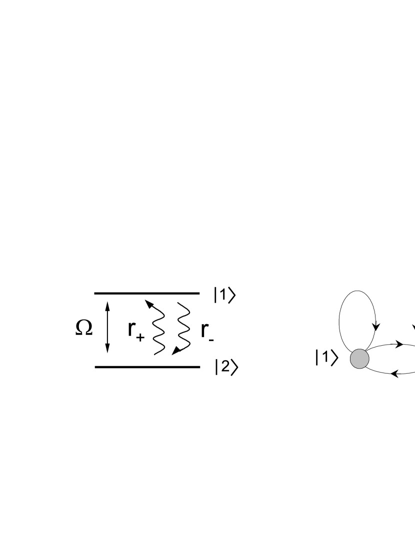
Figure 1: Schematic diagrams of a driven quantum two-level system surrounded by a finite temperature environment and quantum jump trajectories.

III Calculating large deviations of first passage time statistics

We consider an open quantum system with $M$ collapsed quantum states. We assume that a quantum jump trajectory of the system with $N$ collapses starts with a fixed quantum state $\phi_{\eta}$ and that the last collapsed state is $\phi_{\gamma}$. We denote it as

$${\bf X}(t,N)=(\gamma,\alpha_{N-1},\cdots,{\alpha_{2}},{\alpha_{1}},\eta),$$ (1)

where $t$ is the duration of the trajectory, ${\alpha_{i}}$ is the type of collapsed state that occurs at time $t_{i}$, $i=1,\cdots,N$, and $\alpha_{N}=\gamma$. The time-extensive counting variable in the quantum jump trajectory is

$$C[{\bf X}(t,N)]=\sum_{i=1}^{N}w_{\alpha_{i}\alpha_{i-1}}.$$ (2)

where the coefficient $w_{\alpha_{i-1}\alpha_{i}}$ is a weight and is specified by the collapsed states at the adjacent times $t_{i-1}$ and $t_{i}$. Note that here, $\alpha_{0}$ is $\eta$. Although the weights are arbitrary, in practice, they simply equal $\pm 1$ or $0$. In this paper, we focus on these random variables. In this case, Eq. (2) is always an integer.

III.1 Generating function

We are interested in $F(T|n)$, which is the probability distribution for the counting variable (2) first passing a fixed value $n$ at time $T$, especially in the LDs of the random variable $\tau=T/|n|$. We assume that the distribution satisfies the LD principle [8]:

$$F(T|n)\sim e^{-nI_{+}(\tau)}u(n)+e^{nI_{-}(\tau)}u(-n),$$ (3)

where $I_{\pm}$ are the rate functions as $n$ tends to positive infinity and negative infinity, respectively, and $u(n)$ is the unit step function. We assume that the values of $n$ are positive and negative. It is more convenient to investigate the moment generating function (MGF) than the distribution itself:

$$M_{F}(\nu|n)=\int_{0}^{+\infty}dTF(T|n)e^{-\nu T}.$$ (4)

From the LD principle (3), we have the following approximation:

$$M_{F}(\nu|n) \sim e^{n\psi_{+}(\nu)}u(n)+e^{n\psi_{-}(\nu)}u(-n),$$ (5)

where $\psi_{\pm}$ are the SCGFs and are equal to the Legendre transforms of the rate functions $I_{\pm}$, that is,

$$\psi_{\pm}(\nu)=\mp\min_{\tau}\{\nu\tau+I_{\pm}(\tau)\}.$$ (6)

The presence of a fixed integer makes the calculation of the MGF complex. This difficulty can be circumvented by calculating the $z$-transform of $n$ [26]:

$$Z_{F}(\nu|z)=\sum_{n=-\infty}^{+\infty}\ M_{F}(\nu|n)z^{-n}.$$ (7)

The reason is clear from Eq. (13). We simply call Eq. (7) the generating function. According to Eq. (5), this function is expected to have the following approximation:

$$Z_{F}(\nu|z)\sim\frac{1}{1-z^{-1}e^{\psi_{+}(\nu)}}+\frac{1}{1-ze^{-\psi_{-}(\nu)}}.$$ (8)

Two comments are in order. First, the exponentials of the SCGFs of the FPT distribution are just the two poles of the generating function. Hence, if we obtained these poles, e.g., $z^{*}(\nu)$, we would have

$$\psi_{\pm}(\nu)=\ln z^{*}(\nu).$$ (9)

Second, the validity of Eq. (7) indicates that the region of convergence (ROC) of $Z_{F}$ in the $z$-plane is a circle whose radius is in the range of $\exp[\psi_{+}(\nu)]$ to $\exp[\psi_{-}(\nu)]$ [26]. We emphasize that Eq. (9) does not imply that the SCGFs are simply solved from the algebraic equation of the generating function because the number of poles could be more than two. Further analyses are needed .

III.2 Equation of poles

Here, we show how to calculate the generating function $Z_{F}$ of the open quantum system. We let $T_{\alpha\beta}(n|t)$ be the joint transition probability that the quantum system starts from quantum state $\phi_{\beta}$, the last collapsed state is $\phi_{\alpha}$, and the counting variable (2) is $n$ at time $t$, simultaneously. We let $F_{\alpha}(T|n)$ be the FPT distribution of the counting variable passing through $n$ at time $T$ and the last collapsed state being $\phi_{\alpha}$. Obviously,

$$F(T|n)=\sum_{\alpha=1}^{M}F_{\alpha}(T|n).$$ (10)

Note the difference between $t$ and $T$: the former is a fixed duration of the quantum process, whereas the latter is a random variable. Saito and Dhar [11] and Ptaszynski [28] argued that the probabilities satisfy the following equation:

$$\sum_{\beta=1}^{M}{\hat{T}}_{\alpha\beta}(n|\nu)P_{\beta}(0)=\sum_{\gamma=1}^{M}\hat{T}_{\alpha\gamma}(0|\nu){\hat{F}}_{\gamma}(\nu|n),$$ (11)

where $P_{\beta}(0)$ is the probability of the quantum system being in state $\phi_{\beta}$ initially. In the remainder of this paper, we use a “hat” placed over a symbol to denote the Laplace transform with respect to time $t$. Further applying the $z$-transforms of $n$ to both sides of Eq. (11) yields

$$\sum_{\beta=1}^{M}{\bar{\hat{T}}}_{\alpha\beta}(z|\nu)P_{\beta}(0)=\sum_{\gamma=1}^{M}\hat{T}_{\alpha\gamma}(0|\nu){\bar{\hat{F}}}_{\gamma}(\nu|z).$$ (12)

Here, we place a “bar” over a symbol to denote the z-transform of the discrete $n$. Equation (12) is more concise when it is written in matrix form:

$$\bar{\hat{{\mathbb{T}}}}(z|\nu){\bf P}(0)={\hat{{\mathbb{T}}}}(0|\nu){\bar{\hat{\bf F}}}(\nu|z),$$ (13)

where we use a symbol in bold font to indicate a column matrix, e.g., $[{\bf P}(0)]_{\alpha}=P_{\alpha}(0)$, and use a symbol in blackboard bold to indicate a matrix, e.g., $[{\bar{\hat{{\mathbb{T}}}}}]_{\alpha\beta}=\bar{\hat{T}}_{\alpha\beta}$. By substituting Eq. (37) of the counting statistics into Eq. (13), we arrive at the final expression for the generating function of the FPT distribution:

$$Z_{F}(\nu|z) = {\bf 1}^{T}{\bar{\hat{\bf F}}}(\nu|z)$$ (14)

$$= {\bf 1}^{T}{\hat{{\mathbb{T}}}^{-1}(0|\nu)}\hat{{\mathbb{S}}}(\nu){\left[{\mathbb{I}}-{\mathbb{W}}(\nu,z)\right]^{-1}}{\bf P}(0),$$

where the row matrix is ${\bf 1}^{T}=(1\cdots,1)$, superscript $T$ denotes the transpose, and ${\mathbb{I}}$ is the unit matrix. In Eq. (14), the elements of the matrices $\mathbb{W}$ and $\mathbb{S}$ are

$$[{\mathbb{W}}]_{\alpha\beta}=\hat{p}_{\alpha|\beta}(\nu)z^{-w_{\alpha\beta}}$$ (15)

and

$$[\hat{{\mathbb{S}}}]_{\alpha\beta}={\hat{S}}_{\alpha}(\nu)\delta_{\alpha\beta},$$ (16)

respectively, where $\delta_{\alpha\beta}$ is the Kronecker delta symbol. In the former equation, $\hat{p}_{\alpha|\beta}(\nu)$ is the Laplace transform of the WTD $p_{\alpha|\beta}(t)$ for the system starting from the quantum state $\phi_{\beta}$, continuously evolving, and then collapsing to the quantum state $\phi_{\alpha}$ at age $t$. In the latter equation, $\hat{S}_{\alpha}(\nu)$ is the Laplace transform of the survival distribution (SD) $S_{\alpha}(t)$ for the system starting from the quantum state $\phi_{\beta}$ and continuously evolving until time $t$ without collapse. The matrix element $\bar{\hat{T}}_{\alpha\beta}$ is explained in Appendix A. The preceding discussion clearly shows that the generating function $Z_{F}$ is rational, i.e., a ratio of polynomials in $z$. Therefore, the inverse $z$-transform or the MGF $M_{F}(\nu|n)$ must be a linear combination of the right-sided ($\propto u(n)$) and left-sided ($\propto u(-n)$) exponentials [26], the bases of which are determined by the poles and the latter satisfy the following algebraic equation:

$$\det[{\mathbb{I}}-{\mathbb{W}}(\nu,z)]=0.$$ (17)

This is the main result of this work. We call this the equation of poles. Because the ROC of a rational $z$-transform is always bounded by its two poles and does not contain any poles [26], the inverse $z$-transforms for the other poles with smaller magnitude than the left-bounded pole are the right-sided exponentials, whereas the inverse $z$-transforms for the other poles with larger magnitude than the right-bounded pole are the left-sided exponentials. According to the LD principle [8], the terms on the right-hand side of Eq. (5) are the dominant functions of the MGF when $|n|$ tends to infinity. Therefore, we arrive at a key conclusion that $z^{*}$ in Eq. (9) are just the right-bounded and left-bounded poles of the ROC. Crucially, these bounded poles are also given by the valid condition of Eq. (14) that the convergence radius of the matrix $\mathbb{W}$ must be less than 1. Thus far, the value $n$ of the counting variable (2) has been assumed to be positive and negative. If the value of a counting variable is always nonnegative, the previous discussion is slightly modified to adapt to the new situation. Here, we do not present this procedure because of its simplicity. We emphasize that only the terms with subscript $+$ in Eqs. (3)-(9) are currently involved.

Before closing this section, we comment on the known conjugation relationship between the LDs of the FTP and the counting statistics [14] in the quantum case. We have proven that the SCGF of the counting statistics is obtained by solving for the largest real root of the same equation of poles (17) with respect to $\nu$ instead of $\lambda$; see Appendix A. Because both statistics are based on the same ROC, the corresponding SCGFs are indeed inverse functions of each other. Notably, the degrees of the algebraic equation could be distinct with respect to $z$ and $\nu$. This distinction is exploited when we attempt to analytically solve for the LDs of the FPT statistics in the quantum TLS.

IV Quantum Two-Level System

We use the typical quantum TLS to illustrate the previous theoretical results. This system is driven by a resonant field and is surrounded by an environment with inverse temperature $\beta$; see the schematic diagram in the left column of Fig. (1). In the interaction picture, the quantum master equation of the system is

$$\partial_{t}\rho(t) = -{\rm i}\left[H,\rho(t)\right]+r_{-}[\sigma_{-}\rho(t)\sigma_{+}-\frac{1}{2}\{\sigma_{+}\sigma_{-},\rho(t)\}]$$ (18)

$$+r_{+}[\sigma_{+}\rho(t)\sigma_{-}-\frac{1}{2}\{\sigma_{-}\sigma_{+},\rho(t)\}].$$

Here, the Planck constant $\hbar$ is set to 1, $H=-\Omega(\sigma_{-}+\sigma_{+})/2$ represents the interaction Hamiltonian between the TLS and the resonant field, $\sigma_{\pm}$ represents the raising and lowering Pauli operators, and $\Omega$ represents the Rabi frequency. The coefficients $r_{-}=r_{0}(\bar{n}+1)$ and $r_{+}=r_{0}{\bar{n}}$ are the pumping and damping rates, respectively, where $r_{0}$ is the spontaneous decay rate and $\bar{n}$ is the Bose–Einstein distribution of the environment. The two rates satisfy the detailed balance condition $r_{-}=r_{+}\exp{(\beta\omega_{0})}$, and $\omega_{0}$ is the energy level difference. Obviously, the excited state $|1\rangle$ and the ground state $|2\rangle$ are the two collapsed quantum states. Then, the equation of pole (17) is simply

$$[1-\hat{p}_{1|1}(\nu)z^{-w_{11}}][1-\hat{p}_{2|2}(\nu)z^{-w_{22}}]-\hat{p}_{2|1}(\nu)\hat{p}_{1|2}(\nu)z^{-w_{12}-w_{21}}=0.$$ (19)

The Laplace transforms of the WTDs of the system are exactly known [1]. Considering that they are useful in the calculations, we list them at the end of Appendix B.

IV.1 Two exact large deviations of first passage time distributions

We consider two counting variables and solve for their respective SCGFs for the FPT statistics. The first is the number of collapses to the quantum state $|2\rangle$, that is, $w_{21}=w_{22}=1$ and $w_{11}=w_{12}=0$. In quantum optics, collapses to the ground state indicate emissions of photons. Hence, this variable is also interpreted as a count of single photons [24]. Note that its value is nonnegative. By substituting the Laplace transforms of the WTDs $p_{\alpha|\beta}$ for $\alpha,\beta=1,2$ into Eq. (19), simple algebraic operations lead us to

$$[2r_{+}r_{-}\xi(\nu)+r_{-}\Omega^{2}]z^{-1}-2\xi(\nu)[\xi^{2}(\nu)+4\mu^{2}]+r_{+}\Omega^{2}=0,$$ (20)

where $\xi(\nu)=\nu+r/2$, $r=r_{-}+r_{+}$, $16\mu^{2}=4\Omega^{2}-\delta^{2}$, and $\delta=r_{-}-r_{+}$. According to Eq. (9), the SCGF is then simply

$$\psi_{+}(\nu)=\ln\frac{2r_{+}r_{-}\xi(\nu)+r_{-}\Omega^{2}}{2\xi(\nu)[\xi^{2}(\nu)+4\mu^{2}]-r_{+}\Omega^{2}}.$$ (21)

The weights of the second counting variable are $w_{21}=w_{22}=1$ and $w_{11}=w_{12}=-1$. Now, its value can be positive or negative. If we multiply it $\omega_{0}$, the resulting quantity will be the heat of a quantum jump trajectory [29, 30]. Simple algebraic operators of Eq. (19) yields

$$z^{-2}-2b(\nu)z^{-1}+r_{+}/r_{-}=0,$$ (22)

where the coefficient $b(\nu)=\left[\xi^{3}(\nu)+\xi(\nu)(4\mu^{2}-r_{-}r_{+})\right]/\Omega^{2}r_{-}$. This is a quadratic equation in $z$. Then, the two SCGFs of the FPT statistics are

$$\psi_{\pm}(\nu)=-\ln\left[b(\nu)\pm\sqrt{b^{2}(\nu)-r_{+}/r_{-}}\right],$$ (23)

respectively. Because the two rates $r_{\pm}$ satisfy the detailed balance condition, we easily prove that the two SCGFs (23) satisfy the fluctuation theorem

$$\psi_{+}(\nu)=\beta\omega_{0}-\psi_{-}(\nu).$$ (24)

We depict these three SCGFs in Fig. (2)(a) and (b) for a set of parameters.

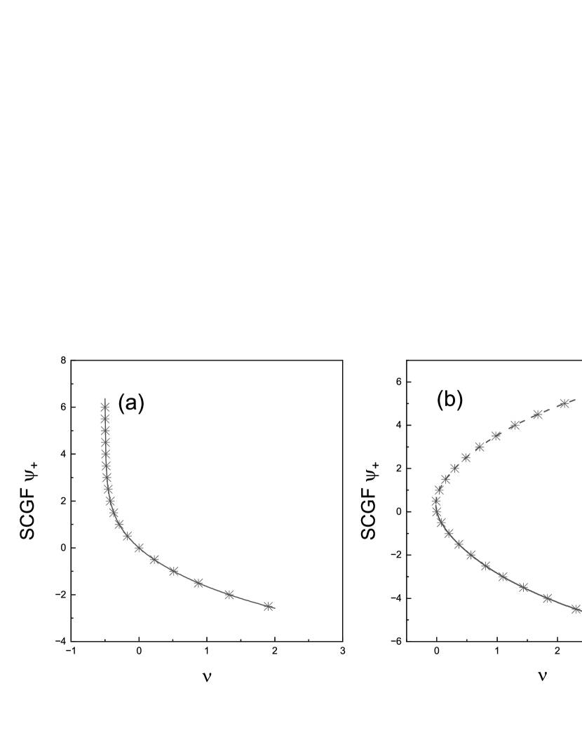
Figure 2: (a) The solid curve is the SCGF $\psi_{+}(\nu)$ of the variable that counts collapses to the ground state. (b) The solid curve and dashed curves are the SCGFs $\psi_{+}(\nu)$ and $\psi_{-}(\nu)$ of the other counting variable, respectively. This random variable is related to the heat production of the quantum jump trajectory. In both panels, the physical parameters are $\omega_{0}=1$, $r_{-}=1$, $r_{+}=0.5$, and $\Omega=0.8$. The star symbols denote the inverse functions of the SCGFs of the counting statistics for the same counting variables.

IV.2 An inverse function method for calculating large deviations of counting statistics

The SCGFs in Fig. (2) can be verified by depicting the inverse functions of the SCGFs of the counting statistics for the same counting variables. As we noted at the end of Sec. (III), the latter are obtained by solving for the largest real roots of Eqs. (20) and (22) with respect to $\nu$ (a function of $\lambda$) [1]; see the star symbols in Fig. (2). Obviously, the degrees of the polynomials of the FPT and counting statistics are distinct: the former are $1$ and $2$, whereas the latter are all 3. This inspires us to use a numerical method to solve for the LDs of the counting statistics in certain quantum systems. If the degree of the equation of poles of $z$ is less than or equal to 3 and far smaller than that of $\nu$, we can first analytically solve the SCGFs $\psi_{\pm}(\nu)$ of the FPT statistics and then perform an inverse function transform, i.e., exchange the positions of $\nu$ and $\psi_{\pm}$ to obtain the SCGFs of the counting statistics. An advantage of this method is that it avoids the procedure of finding the largest real roots of higher-degree polynomials . For example, in the quantum three-level system with one collapsed quantum state that is schematically shown in Fig. (3), the degree of the equation of poles of $\nu$ is 6. In contrast, the degree of the same equation of $z$ is $1$ [3]. We test the method in the system, and the data are very satisfactory; see Fig. (3).

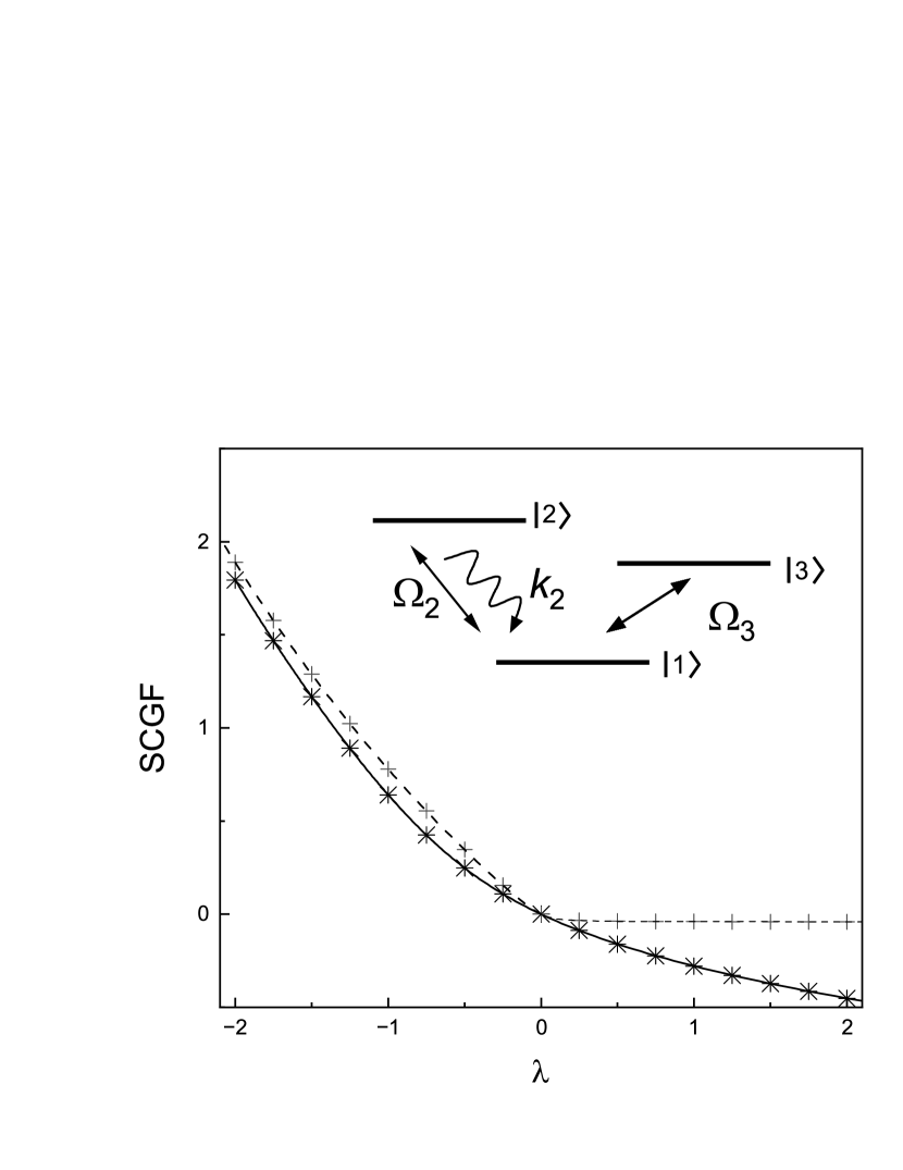
Figure 3: Schematic diagram of a driven quantum three-level system with one collapsed quantum state $|1\rangle$ and the SCGFs of the counting statistics for the random variable counting the number of collapses to the state $|1\rangle$. The star and cross symbols represent the SCGF data obtained by solving for the largest real root of a 6-degree polynomial, where two sets of physical parameters are used [3]. The solid and dashed curves represent the SCGF data obtained via the inverse function method. Note that the features of the SCGFs depend on the values of the parameters [3, 16].

IV.3 Violations of classical uncertainty relations

In the past several years, quantum violations of the classical thermodynamic uncertainty relation (TUR) [32, 33] and kinetic uncertainty relation (KUR) [12] have attracted much interest. [34, 35, 36, 37, 38, 9, 39, 40]. Because Gingrich and Horowitz noted that both uncertainty relations are conjugated in the counting statistics and FPT statistics [14], we are interested in applying the exact SCGFs, Eqs. (21) and (23), to study the same question. The first is the classical KUR [41]. Its conjugation in the FPT statistics written in terms of the SCGF is

$$-\left.\frac{\psi_{+}^{\prime\prime}}{\psi_{+}^{\prime}}\right|_{\nu=0}\geq\frac{1}{\langle k\rangle},$$ (25)

where $\langle k\rangle$ represents the mean activity and prime (^′) and double prime (^′′) denote the first and second derivatives with respect to $\nu$, respectively. Here, the random counting variable of interest is the number of collapses to the ground state $|2\rangle$. On the basis of Eq. (21), we easily calculate the left-hand side of Eq. (25), and the result is

$$\frac{2\Omega^{2}+r^{2}+4r_{+}r_{-}}{r_{-}(\Omega^{2}+rr_{+})}-\frac{6r}{2\Omega^{2}+r^{2}}.$$ (26)

The mean activity is equal to the reciprocal of the mean random variable $\langle T/K\rangle$ in the large $K$ limit, where $K$ is the full counting variable. We let the SCGF of the FPT statistics of the full counting variable be $\psi_{k}(\nu)$. The corresponding equation of poles is obtained by setting $w_{ij}=1$ for $i,j=1,2$ in Eq. (2), that is,

$$2r_{+}r_{-}\xi z^{-2}+\Omega^{2}rz^{-1}-2\xi(\xi^{2}+4\mu^{2})=0.$$ (27)

Then, the right-hand side of Eq. (25), or the classical kinetic bound, is

$$\frac{1}{\langle k\rangle}=-\psi_{k}^{\prime}(0)=\frac{2\Omega^{2}+r^{2}}{r(\Omega^{2}+2r_{+}r_{-})}.$$ (28)

In Fig. (4)(a), using two independent dimensionless parameters, $r_{0}/\Omega$ and $\bar{n}$, we numerically depict the exact curve on which the inequality (25) reduces to an equality. We see that quantum violation of the KUR is not uncommon in the parameter space; see the shaded area therein. Equations (26) and (28) simply explain the validity of the KUR at very small and large $r_{0}/\Omega$. If the Rabi frequency is very large, $\it i.e.$, $r_{0}/\Omega\ll 1$, the two equations are approximately $1/r_{-}$ and $1/r$, respectively. Obviously, $1/r_{-}>1/r$. If the Rabi frequency is very small, $\it i.e.$, $r_{0}/\Omega\gg 1$, the two equations are approximately the equations for the classical KUR in an incoherent TLS. Under this situation, the inequality must be valid [12]. An algebra also proves this. Note that these two cases are independent of $\bar{n}$. We see that quantum violations of the KUR mainly occurs at smaller $\bar{n}$ and intermediate Rabi frequencies. To illustrate this observation, in Fig. (4)(b), we specifically depict Eqs. (26) and (28) as functions of $r_{0}/\Omega$ at fixed $\bar{n}=0.15$. There are two quantum bounds for the KUR in the literature. On the basis of the sMP perspective on quantum jump trajectories, Carollo et al. derived a factor $\chi$ to replace the mean activity [9],

$$\chi=\sum_{\alpha,\beta=1}^{2}\frac{\sigma^{2}_{\beta\alpha}}{\tau^{2}_{\beta\alpha}}R_{\beta\alpha}c_{\alpha}.$$ (29)

The precise meanings of the involved coefficients are discussed in Appendix B. We show the numerical data for the quantum bound $1/\chi$ in Fig. (4)(b); see the dashed curve. Another interesting quantum bound was proposed by Van Yu and Saito [38]. They corrected the mean activity to

$$\langle k\rangle+Q=\langle k\rangle\left(1+\frac{8\Omega^{2}}{r^{2}}\right).$$ (30)

Considering that Ref. [40] presented a careful derivation, we do not explain the correction but only directly present the final expression. We depict the quantum bound $1/(\langle k\rangle+Q)$ in Fig. (4)(b); see the dotted curve therein. We see that these two quantum bounds are always valid. In particular, they uniformly converge to the classical bound at larger $r_{0}/\Omega$, that is, that of the incoherent TLS. At a larger Rabi frequency, however, their predictions completely deviate. Apparently, the bound of Eq. (29) is better than the bound of Eq. (30).

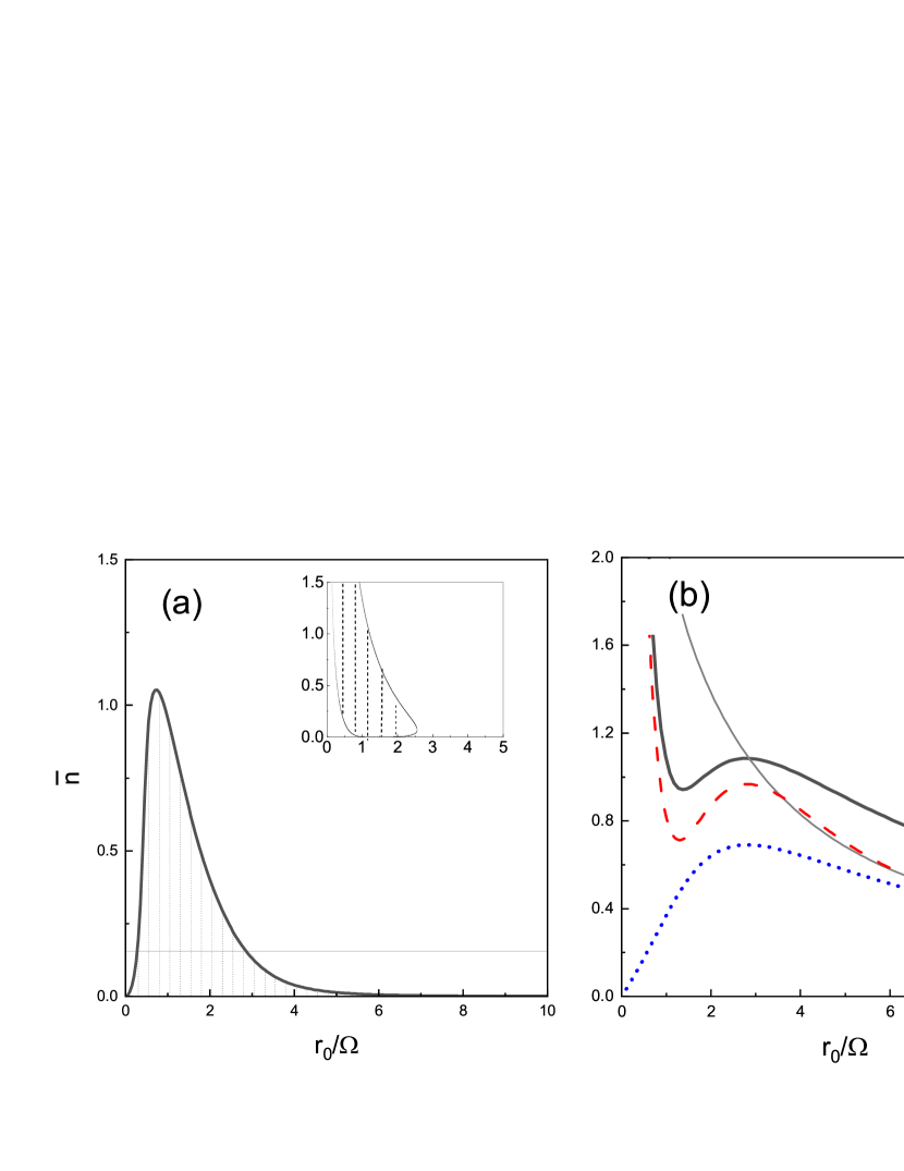
Figure 4: (a) The curve indicates the values of $r_{0}/\Omega$ ($x$-axis) and $\bar{n}$ ($y$-axis) on which the classical KUR of the quantum TLS reduces to equality. The uncertainty relation is violated in the area enclosed by the curve and $x$-axis. The $\bar{n}$ value of the horizontal line is $0.15$. The inset shows the curve on which the classical TUR of the same quantum system reduces to equality. (b) The black solid curve and gray thin curve represent the data calculated using the left-hand side and right-hand side (the classical bound) of the classical KUR, Eqs. (26) and (28), respectively. The dashed and dotted curves are the quantum bounds $1/\chi$ and $1/(\langle k\rangle+Q)$, respectively.

We briefly discuss the classical TUR to close this work. The classical TUR of an asymmetric current in the FPT statistics

expressed in terms of the SCGF is [14]

$$-\left.\frac{\psi_{+}^{\prime\prime}}{\psi_{+}^{\prime}}\right|_{\nu=0}\geq\frac{2k_{B}}{\langle\sigma\rangle},$$ (31)

where $k_{B}$ is the Boltzmann constant, $\langle\sigma\rangle$ is the mean entropy production rate, and we assume that the mean current is positive. The rate of the second counting variable mentioned in Sec. (IV.1) is an asymmetric current of the quantum TLS. Accordingly, the general Eq. (31) is reduced to

$$\beta\omega_{0}\left.\frac{\psi^{\prime\prime}_{+}}{(\psi^{\prime}_{+})^{2}}\right|_{\nu=0}\geq 2.$$ (32)

Here, we use the relation $k_{B}/\langle\sigma\rangle=-\psi_{+}^{\prime}(0)/\beta\omega_{0}$. By substituting the exact Eq. (23) and performing simple algebraic operations, we obtain the left-hand side of Eq. (32):

$$\beta\omega_{0}\left[\frac{r}{\delta}-\frac{6\Omega^{2}\delta r}{(2\Omega^{2}+r^{2})^{2}}\right].$$ (33)

Similar to the case of the KUR, using the parameters $r_{0}/\Omega$ and $\bar{n}$, we numerically determine the curve on which the inequality (32) reduces to an equality; see the inset of Fig. (4)(a). We find that violation of the classical TUR is also not uncommon. In particular, the area of violation is very distinct from that in which the classical KUR is satisfied. Menczel et al.. [36] investigated the causes of the violation in detail. They also obtained the same Eq. (33) as a special case of a general equation in the presence of detuning; see Eq. (10) therein. Note that the preceding derivations were carried out for the counting statistics, in which a characteristic polynomial technique was used [17]. Therefore, this consistency again demonstrates the conjugation between these two statistics.

V Discussion and Conclusions

In this paper, we apply the sMP method to calculate the large deviations of the FPT statistics in open quantum systems. We find that the SCGFs can be obtained by solving an algebraic equation of poles and calculating the logarithm of the solution. Because the same equation is used to solve for the SCGFs of the counting statistics for the same counting variables, the conclusion that large deviations of the FPT statistics and counting statistics are conjugated and connected by inverse functions to each other is explicitly obtained in the quantum regime. An intriguing finding of this paper is that the degrees of the equation of poles are distinct with respect to the two statistics, at least in the typical quantum system with which we are concerned. Because the degree of the polynomial for the FPT statistics is usually smaller than that for the counting statistics, analytically solving for the former SCGFs is possible. Hence, instead of the conclusion that one should first solve for the large deviations of the counting statistics and then obtain the large deviations of the FPT statistics through the inverse function, our result indicates that a converse procedure is more useful in open quantum systems. In addition, we use the analytical SCGFs of the FPT statistics to explore quantum violations of the classical KUR and TUR. The relationships between the two statistics are shown again. Intriguingly, the quantum bound based on the sMP perspective is tighter than other quantum bounds are. Clarifying the cause and its implications for quantum TUR deserves further investigation. We hope that in the near future, we will report this progress.

Acknowledgments This work was supported by the National Natural Science Foundation of China under Grants No. 12075016 and 11575016.

Appendix A Joint transition probabilities of counting statistics

In terms of the WTDs, the probability distribution of the trajectory (1) is

$${\cal P}[{\bf X}(t,N)]=S_{\gamma}(t-t_{N})p_{\gamma|\alpha_{N-1}}(t_{N}-t_{N-1})\cdots p_{\alpha_{2}|\alpha_{1}}(t_{2}-t_{1})p_{\alpha_{1}|\eta}(t_{1}),$$ (34)

where the first term on the right-hand side of the equation is the SD

$$S_{\gamma}(t)=\int_{t}^{\infty}\sum_{\beta=1}^{M}p_{\beta|\gamma}(s)ds.$$ (35)

The joint transition probability of the counting variable (2) is formally expressed by the trajectory distribution as

$$T_{\gamma\eta}(n|t)=\sum_{N=0}^{\infty}\sum_{{\bf X}(t,N)}{\cal P}[{\bf X}(t,N)]\delta_{nC[{\bf X}(t,N)]}.$$ (36)

Note that the second summation is presented in shorthand notation: it represents the sums of all possible intermediate collapsed states $\phi_{\alpha_{i}}$ and integrals for all times $t_{i}$, $0\leq t_{1}\leq\cdots\leq t_{N}\leq t$. Equation (36) is complex. However, it can be dramatically simplified by calculating the Laplace transform of time $t$ and the $z$-transform of count $n$ simultaneously. The result is

$$\bar{\hat{T}}_{\gamma\eta}(z|\nu) = {\hat{S}}_{\gamma}(\nu)\sum_{N=0}^{\infty}{\hat{p}}_{\gamma|\alpha_{N-1}}(\nu)z^{-w_{\gamma\alpha_{N-1}}}\cdots{\hat{p}}_{\alpha_{2}|\alpha_{1}}(\nu)z^{-w_{\alpha_{2}\alpha_{1}}}{\hat{p}}_{\alpha_{1}|\eta}(\nu)z^{-w_{\alpha_{1}\eta}}$$ (37)

$$= \left[\hat{{\mathbb{S}}}(\nu)\sum_{N=0}^{\infty}{\mathbb{W}}^{N}(\nu,z)\right]_{\gamma\eta}$$

$$= \left[\hat{{\mathbb{S}}}(\nu)\hskip 2.84544pt\left(\mathbb{I-W}(\nu,z)\right)^{-1}\right]_{\gamma\eta}.$$

Here, we defined an $M\times M$ matrix $\mathbb{W}$ and diagonal matrix $\hat{\mathbb{S}}$, and their elements are given in Eqs. (15) and (16), respectively. We emphasize that the spectral radius of the matrix $\mathbb{W}$ must be less than $1$ to ensure convergence of the sum of the power matrices. In our preceding paper [1], we defined a matrix $\mathbb{G}$ to calculate the generating function of the counting statistics:

$$Z_{C}(z|\nu) = {\bf 1}^{T}{\mathbb{G}}^{-1}(z,\nu){\bf P}(0),$$ (38)

where $z=\exp(\lambda)$ and $\lambda$ are the parameters of the counting statistics of the counting variable (2). The elements of the matrix $\mathbb{G}$ are

$$[{\mathbb{G}}]_{\gamma\gamma} = \frac{1-\hat{p}_{\gamma|\gamma}(\nu)z^{-w_{\gamma\gamma}}}{\hat{S}_{\gamma}(\nu)}$$ (39)

$${\rm}[{\mathbb{G}}]_{\gamma\eta} = -\frac{\hat{p}_{\gamma|\eta}(\nu)z^{-w_{\gamma\eta}}}{\hat{S}_{\gamma}(\nu)},{\hskip 2.84544pt}\gamma\neq\eta,$$ (40)

respectively. It is easy to see that

$${\mathbb{G}}(\nu,z)=\left[\mathbb{I-W}(\nu,z)\right]{\hat{\mathbb{S}}}^{-1}(\nu),$$ (41)

and the matrix ${\mathbb{G}}^{-1}$ is just the joint transition probability matrix $\mathbb{T}$ for the counting statistics. Several comments are on order. First, Eq. (38) is a quantum extension of the equation derived by Andrieux and Gaspard many years ago when they studied the current fluctuation theorem in the classical sMPs of classical stochastic systems [42]. Second, Eq. (41) implies that the SCGF of the counting statistics is obtained by solving the same equation of pole (17) with respect to $\nu$ (a function of $\lambda$). Finally, there is still another expression for the matrix $\mathbb{G}$:

$${\mathbb{G}}(z,\nu) = \nu{\mathbb{I}}-{\mathbb{L}}(z,\nu)$$ (42)

where the elements of the matrix $\mathbb{L}$ are

$$[{\mathbb{L}}]_{\gamma\gamma} = \frac{\hat{p}_{\gamma|\gamma}(\nu)z^{-\omega_{\gamma\gamma}}-\sum_{\alpha=1}^{M}{\hat{p}}_{\alpha|\gamma}(\nu)}{\hat{S}_{\gamma}(\nu)}$$ (43)

and $[{\mathbb{L}}]_{\gamma\eta}=[{\mathbb{G}}]_{\gamma\eta}$, with $\gamma\neq\eta$. The matrix $\mathbb{L}$ is the quantum extension [1] of the tilted generator of a classical sMP [43]. If all the weights $w_{\gamma\eta}$ and diagonal elements ${\hat{p}}_{\gamma\gamma}$ are zero, this matrix reduces to the standard generator of the sMP in the frequency domain [44].

Appendix B The factor $\chi$ of Carollo et al. [9]

In Eq. (29), the coefficients $c_{\alpha}$ for $\alpha=1,2$ represent the rates of the quantum system collapsing into quantum state $\phi_{\alpha}$ in the steady state. They can be written in terms of the Laplace transforms of the WTDs [1, 9] as

$$c_{1} = \left.\frac{{\hat{p}}_{12}}{{\hat{p}}_{12}\tau_{1}+{\hat{p}}_{21}\tau_{2}}\right|_{\nu=0},$$ (44)

$$c_{2} = \left.\frac{{\hat{p}}_{21}}{{\hat{p}}_{12}\tau_{1}+{\hat{p}}_{21}\tau_{2}}\right|_{\nu=0},$$ (45)

where $\tau_{\alpha}={\hat{p}}^{\prime}_{1\alpha}+{\hat{p}}^{\prime}_{2\alpha}$ is the mean time of the quantum system starting from quantum state $\phi_{\alpha}$ and continuously evolving without collapse, that is, the mean age of deterministic evolution. The coefficient $R_{\beta\alpha}$ is the transition probability of a Markov chain embedded in the sMP, which is simply equal to $\left.\hat{p}_{\beta\alpha}\right|_{\nu=0}$. The coefficients $\sigma^{2}_{\beta\alpha}$ and $\tau_{\beta\alpha}$ are the variance and mean of the time that the quantum system starts from the quantum state $\phi_{\alpha}$ and finally collapses to state $\phi_{\beta}$, respectively [9]. Their ratio is

$$\frac{\sigma^{2}_{\beta\alpha}}{\tau^{2}_{\beta\alpha}}=\left.\frac{{\hat{p}}^{\prime\prime}_{\beta\alpha}{\hat{p}}_{\beta\alpha}}{\hat{p}^{\prime 2}_{\beta\alpha}}\right|_{\nu=0}-1.$$ (46)

By substituting the exact formulas for the Laplace transforms of the WTDs of the quantum TLS [1], we can obtain exact expressions for each term in Eq. (29). Because this is a straightforward procedure and several expressions are lengthy, we do not present them here. To make this paper self-contained, the Laplace transforms of the WTDs of the quantum TLS are listed below:

$$\hat{p}_{1|1}(\nu) = r_{+}\frac{\Omega^{2}}{2\xi(\nu)[\xi^{2}(\nu)+4\mu^{2}]},$$

$$\hat{p}_{1|2}(\nu) = r_{+}\frac{\xi^{2}(\nu)+\delta\xi(\nu)/2+\Omega^{2}/2}{\xi(\nu)[\xi^{2}(\nu)+4\mu^{2}]}$$

$$\hat{p}_{2|1}(\nu) = r_{-}\frac{\xi^{2}(\nu)-\delta\xi(\nu)/2+\Omega^{2}/2}{\xi(\nu)[\xi^{2}(\nu)+4\mu^{2}]},$$

$$\hat{p}_{2|2}(\nu) = r_{-}\frac{\Omega^{2}}{2\xi(\nu)[\xi^{2}(\nu)+4\mu^{2}]}.$$ (47)

References

- [1] Fei Liu. Semi-markov processes in open quantum systems: Connections and applications in counting statistics. Phys. Rev. E, 106:054152, Nov 2022.
- [2] Fei Liu. Semi-markov processes in open quantum systems. ii. counting statistics with resetting. Phys. Rev. E, 108:064101, Dec 2023.
- [3] Fei Liu. Asymptotic large deviations of counting statistics in open quantum systems. Phys. Rev. E, 108:064111, Dec 2023.
- [4] Lee H. Levitov, L. S. and G. B Lesovik. Electron counting statistics and coherent states of electric current. J. Math. Phys, 1996.
- [5] D. A. Bagrets and Yu. V. Nazarov. Full counting statistics of charge transfer in coulomb blockade systems. Phys. Rev. B, 67:085316, Feb 2003.
- [6] Massimiliano Esposito, Upendra Harbola, and Shaul Mukamel. Nonequilibrium fluctuations, fluctuation theorems, and counting statistics in quantum systems. Rev. Mod. Phys., 81(4):1665, 2009.
- [7] Samuel L. Rudge and Daniel S. Kosov. Counting quantum jumps: A summary and comparison of fixed-time and fluctuating-time statistics in electron transport. J. Chem. Phys., 151(3), 07 2019. 034107.
- [8] Hugo Touchette. The large deviation approach to statistical mechanics. Phys. Rep., 478(1-3):1–69, 2008.
- [9] Federico Carollo, Robert L. Jack, and Juan P. Garrahan. Unraveling the large deviation statistics of markovian open quantum systems. Phys. Rev. Lett., 122(13):130605, April 2019.
- [10] Calum A. Brown, Katarzyna Macieszczak, and Robert L. Jack. Unraveling metastable markovian open quantum systems. Phys. Rev. A, 109:022244, Feb 2024.
- [11] K. Saito and A. Dhar. Waiting for rare entropic fluctuations. Europhys. Lett., 2016.
- [12] Juan P. Garrahan. Simple bounds on fluctuations and uncertainty relations for first-passage times of counting observables. Phys. Rev. E, 95:032134, Mar 2017.
- [13] Todd R Gingrich, Grant M Rotskoff, and Jordan M Horowitz. Inferring dissipation from current fluctuations. Journal of Physics A: Mathematical and Theoretical, 50(18):184004, April 2017.
- [14] Todd R. Gingrich and Jordan M. Horowitz. Fundamental bounds on first passage time fluctuations for currents. Phys. Rev. Lett., 119:170601, Oct 2017.
- [15] Joel L. Lebowitz and Herbert Spohn. J. Stat. Phys., 95(1/2):333–365, 1999.
- [16] Juan P. Garrahan and Igor Lesanovsky. Thermodynamics of quantum jump trajectories. Phys. Rev. Lett., 104(16):160601, Apr 2010.
- [17] M. Bruderer, L. D. Contreras-Pulido, M. Thaller, L. Sironi, D. Obreschkow, and M. B. Plenio. Inverse counting statistics for stochastic and open quantum systems: the characteristic polynomial approach. New J. Phys., 16 (2014)(3):033030, 2014.
- [18] Heinz-Peter Breuer and Francesco Petruccione. The theory of open quantum systems. Oxford university press, 2002.
- [19] B. R. Mollow. Pure-state analysis of resonant light scattering: Radiative damping, saturation, and multiphoton effects. Phys. Rev. A, 12:1919–1943, Nov 1975.
- [20] P. Zoller, M. Marte, and D. F. Walls. Quantum jumps in atomic systems. Phys. Rev. A, 35:198–207, Jan 1987.
- [21] M.D. Srinivas and E.B. Davies. Photon counting probabilities in quantum optics. Opt. Acta., 28(7):981–996, 1981.
- [22] Howard Carmichael. An open systems approach to Quantum Optics, volume 18. Springer, 1993.
- [23] Klaus Mølmer, Yvan Castin, and Jean Dalibard. Monte carlo wave-function method in quantum optics. J. Opt. Soc. Am. B, 10(3):524–538, Mar 1993.
- [24] M.B. Plenio and P.L. Knight. The quantum-jump approach to dissipative dynamics in quantum optics. Rev. Mod. Phys., 70(1):101, 1998.
- [25] Sheldon M. Ross. Stochastic Processes. John Wiley & Sons, New York, 2nd edition edition, 1995.
- [26] Alan V.oppenheim, Alan S. Willsky, and S. Hamid Nawab. Signals and Systems. Prentice-Hall, Inc.:Upper Saddle River, NJ., 2nd edition edition, 1997.
- [27] In this work, fortunately, the number of poles of the quantum TLS is indeed less than or equal to 2.
- [28] Krzysztof Ptaszyński. First-passage times in renewal and nonrenewal systems. Phys. Rev. E, 97:012127, Jan 2018.
- [29] Heinz-Peter Breuer. Quantum jumps and entropy production. Phys. Rev. A, 68:032105, Sep 2003.
- [30] Fei Liu and Jingyi Xi. Characteristic functions based on a quantum jump trajectory. Phys. Rev. E, 94:062133, Dec 2016.
- [31] Many efficient algorithms exist for finding the roots of polynomials. Nevertheless, our method is simple.
- [32] Andre C. Barato and Udo Seifert. Thermodynamic uncertainty relation for biomolecular processes. Phys. Rev. Lett., 114:158101, Apr 2015.
- [33] Todd R. Gingrich, Jordan M. Horowitz, Nikolay Perunov, and Jeremy L. England. Dissipation bounds all steady-state current fluctuations. Phys. Rev. Lett., 116:120601, Mar 2016.
- [34] Krzysztof Ptaszyński. Coherence-enhanced constancy of a quantum thermoelectric generator. Phys. Rev. B, 98:085425, Aug 2018.
- [35] Obinna Abah and Eric Lutz. Efficiency of heat engines coupled to nonequilibrium reservoirs. EPL (Europhysics Letters), 106(2):20001, April 2014.
- [36] Paul Menczel, Eetu Loisa, Kay Brandner, and Christian Flindt. Thermodynamic uncertainty relations for coherently driven open quantum systems. Journal of Physics A: Mathematical and Theoretical, 54(31):314002, jul 2021.
- [37] Alex Arash Sand Kalaee, Andreas Wacker, and Patrick P. Potts. Violating the thermodynamic uncertainty relation in the three-level maser. Phys. Rev. E, 104:L012103, Jul 2021.
- [38] Tan Van Vu and Keiji Saito. Thermodynamics of precision in markovian open quantum dynamics. Phys. Rev. Lett., 128:140602, Apr 2022.
- [39] Yoshihiko Hasegawa. Quantum thermodynamic uncertainty relation for continuous measurement. Phys. Rev. Lett., 125:050601, Jul 2020.
- [40] Michael J. Kewming, Anthony Kiely, Steve Campbell, and Gabriel T. Landi. First passage times for continuous quantum measurement currents, 2023.
- [41] J. P. Garrahan, R. L. Jack, V. Lecomte, E. Pitard, K. van Duijvendijk, and F. van Wijland. Dynamical first-order phase transition in kinetically constrained models of glasses. Phys. Rev. Lett., 98:195702, May 2007.
- [42] D. Andrieux and P. Gaspard. Fluctuation theorem for currents in semi-markov processes. J. Stat. Mech.: Theor. Exp, page P11007, 2008.
- [43] Massimiliano Esposito, Upendra Harbola, and Shaul Mukamel. Fluctuation theorem for counting statistics in electron transport through quantum junctions. Phys. Rev. B, 75:155316, Apr 2007.
- [44] H. Qian and H. Wang. Continuous time random walks in closed and open single-molecule systems with microscopic reversibility. Europhys. Lett., 76(1):15–21, 2006.