AAA

We show that the near-brane back-reaction of M2 branes ending on M5 branes has a rich “spike structure” that is determined by partitioning the numbers of M2 branes that are terminating on groups of M5 branes. The near-brane limit of the metric describing these branes has an AdS₃ factor, implying the existence of a dual CFT. Each partition of the M2 and M5 charges among spikes gives rise to a different “mohawk” revealing a new layer of brane fractionation. We conjecture that all these mohawks are dual to ground states of near-brane-intersection CFT’s. We show that the supergravity solutions describing these mohawks are part of the large families of AdS₃ $\times S^{3}\times S^{3}$ solutions described in [1]. We identify precisely which of these families are relevant to brane intersections and show that the AdS₃ invariance emerges from the self-similarity of the spikes.

1 Introduction

The study of intersecting brane systems has a vast and diverse history in String Theory. One can gain significant insight by treating the branes perturbatively, or using the brane actions to determine their dynamics, while the fully back-reacted supergravity solutions for intersecting branes can be very challenging. This problem can be simplified by smearing the brane distribution, but this can wipe out essential dynamical details, especially if one is trying to describe black-hole microstructure [2, 3, 4]. Ideally one would like supergravity solutions that describe unsmeared brane intersections, but such solutions typically involve metrics and fluxes that are characterized by complicated systems of non-linear equations.

There are two ways in which such non-linear systems can be rendered manageable. The first is to try to arrange a very high level of symmetry so that the configuration only depends on one or two variables. In this situation, the equations sometimes simplify to a linear system. However, such a high level of symmetry often involves smearing out structures that one wants to investigate. The second approach is to consider some form of “near-brane” limit in which some of the functional dependence of the solution is controlled by scale invariance, while the remaining equations can be reduced to a linear system. In this paper we will make a detailed exploration of an example of such a near-brane limit.

We focus on stacks of M2 and M5 branes that intersect along a common $\mathbb{R}^{1,1}$. The intersection is thus co-dimension $4$ in the M5 branes, and we will impose spherical symmetry in these directions along the stack of M5 branes. The intersecting M2-M5 system also has co-dimension $4$ in the complete space time, and we will also impose spherical symmetry in these transverse directions. The solution therefore has an $\mathbb{R}^{1,1}\times SO(4)\times SO(4)$ symmetry, and depends on three variables, $(u,v,z)$, where $u,v$ are, respectively, radial coordinates in the M5 branes and the transverse space, while $z$ is the remaining coordinate along the M2 branes. This class of brane intersections has been extensively studied, and the general solution is governed by a non-linear Monge-Ampère-like equation [5, 6, 7, 8, 9].

As an offshoot of the study of Janus solutions, a near-brane limit of intersecting M2 and M5 branes was constructed by seeking out solutions with an $SO(2,2)\times SO(4)\times SO(4)$ symmetry [10, 11, 12, 13, 14, 15, 1]. These solutions contain a warped product of AdS₃ $\times S^{3}\times S^{3}$, with the remaining two dimensions described by a Riemann surface, coordinatized by $(\xi,\rho)$. The underlying BPS equations were also simplified to a linear system. In [8] it was shown how a class of these solutions could be mapped onto a near-brane limit of the M2-M5 intersections described in [6, 7]. In particular, it was shown how, in such a limit, the coordinates $(u,v,z)$ can be recast in terms of the scale coordinate, $\mu$, of a Poincaré AdS₃ and the coordinates $(\xi,\rho)$ of the Riemann surface. This work also implicitly implies that, by reducing the problem to only two non-trivial variables, the Monge-Ampère-like system can be reduced to a linear set of equations.

Despite this mapping, it remained unclear what kind of M2-M5 systems the solutions of [1] describe. The complication is that the solutions of [1] involve choices of the Riemann surface and choices of poles and residues in a single function, $G$, that defines the flux sources. These choices are inextricably linked by requiring regularity of the solution. In this paper we will make a detailed analysis of certain families of solutions constructed in [1] and show that they describe, what appears from infinity, to be a single stack of semi-infinite M2 branes ending on, and deforming, a single stack of M5 branes. More precisely, the brane stacks are all coincident at infinity but, because the M2 branes pull on the M5 branes, the back-reaction causes these stacks to resolve into physically separated spikes ( a “mohawk”), with the distance between each spike being controlled by the number of M2’s and M5’s making up each spike.

More generally, we suspect that any near-brane limit that leads to such an AdS₃ factor is necessarily limited to a single intersection. The argument is simple: a more complicated intersection must involve a scale that would violate the symmetries of the AdS₃. Consider, for example, a supergravity solution for an M2 brane stretched between two M5 branes. As we will see, the supergravity solution for a single intersection faithfully reproduces a geometry consistent with the spike created by an F1 ending on a D-brane [16, 17]. An M2 brane stretched between M5’s must look like two spikes that meet one another, as depicted in Fig. 1, creating a two-sided tube between the M5’s. Around this tube there will be a $7$-cycle that is a Gaussian surface for the M2 charge. In the configuration shown in Fig. 1, this $7$-cycle will reach a minimum size at some value of the putative AdS radius. This will break the scale invariance of the AdS.

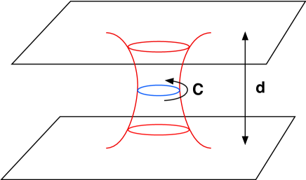
Figure 1: An M2 brane stretched between two M5 branes. In the back-reacted solution, the branes will be stretched and the minimum circumference, $C$, around the M2 branes will depend on the separation, $d$, of the M5 branes.

The near-brane AdS₃ geometries that we investigate are limited to a single intersection, but the solutions are far from being featureless. Once the back-reaction is incorporated via a supergravity solution, we find spikes created by M2 branes ending on M5 branes that have a profile [16, 17, 6]:

$$z~{}\sim~{}\frac{c}{u^{2}}\,.$$ (1.1)

The right-hand side is generically a harmonic function sourced by the M2’s ending on the M5’s, and is thus proportional to $u^{-2}$ given the spherical symmetry. The steepness of the spike, $c$, is determined by the ratio of the number, $Q_{M2}$, of M2 branes that are pulling and the number, $Q_{M5}$, of M5 branes being deformed. Indeed, $c\sim\frac{Q_{M2}}{Q_{M5}}$. However, as we will show, the AdS₃ can accommodate any number of spikes with different steepnesses and the self-similarity of (1.1) is what leads to the scale invariance. Thus we can partition the stack of M5 branes into groups, and choose the number of M2’s that end on each group. This results in different spikes whose steepness is controlled by the value of $\frac{Q_{M2}}{Q_{M5}}$ in each group.

 

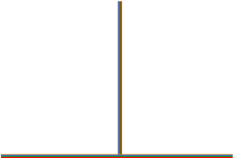
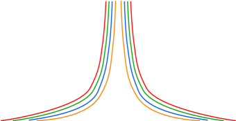
Figure 2: Brane fractionation at a single intersection as a result of back-reacted brane bending. If the bent branes are self-similar, preserving a scale invariance, then the near-brane description can result in an AdS geometry.

Upon turning on the back-reaction, the different groups spatially separate according to their steepness. This is depicted in Fig. 2. The residues of the function, $G$, control the number of M5’s in each group, while the location of the poles of $G$ on the Riemann surface is controlled by the steepness, and thus encodes the M2 charge in each group. In this way, a “single intersection” of non-back-reacted branes actually resolves into a complex of multiple, self-similar intersections whose components localize at different points on the Riemann surface. At infinity, the brane configuration converges to a stack of coincident M5’s in one direction and M2’s in another, but as one zooms into the intersection, the M2’s and M5’s resolve into physically separated groups.

It is interesting to note that this brane picture describes the solutions of [1] that have $AdS_{4}/\mathbb{Z}_{2}$ asymptotics, as well as the solutions that have $AdS_{7}$ asymptotics. The $AdS_{4}/\mathbb{Z}_{2}$ asymptotics is not surprising: after all, as one goes up the semi-infinite M2 branes, far away from the M5 branes, one expects the geometry they source to be $AdS_{4}\times S^{7}$. However, for the asymptotically-$AdS_{7}$ geometries one might naively hope that they describe M2 branes sandwiched between M5 branes [1]. However, as we will discuss in Section 3, these solutions are simply a zoom-in limit at the bottom of the spike depicted in Fig. 2, and hence are degenerate limit of an M2-M5 infinite spike.

In Section 2 we review the known supergravity solutions for M2-M5 intersections, focussing on the geometry that emerges in the near-intersection limit. We follow this, in Section 3, with our primary example because it has all the essential features of a single intersection. In Section 4 we return to the general near-intersection solutions and compute, in detail, the M2-brane charge density function, and evaluate it at all the sources in the example. This gives us the picture of the M2-M5 mohawk: a collection of self-similar spikes separated according to steepness. Section 5 contains some final comments. In Appendix A we show how M5-brane probes reproduce a key characteristic of the mohawk. That is, given a supergravity solution M2-M5 mohawk, one can analyze the forces experienced by a probe component of the mohawk (an M5-brane with an M2 spike, which in the coordinates of [1] is extended along the $AdS_{3}\times S_{3}$ part of the geometry). We show that the probe has an equilibrium position on the boundary of the Riemann surface depends linearly on the amount of M2 flux along the probe world-volume. This implies that the relation between the M2 charge and the steepness of the spike is that same as that in the spikes whose backreaction gives rise to the background $AdS_{3}\times S_{3}\times S_{3}$ solution.

2 General M2-M5 intersections and AdS₃ limits

2.1 General M2-M5 intersections

As described in the Introduction, the brane configuration becomes much clearer in the original formulation of [6, 7], and we follow the discussion in [8, 9]. The M2 directions correspond to the coordinates $(x^{0},x^{1},x^{2})=(t,y,z)$, while the coordinates along the M5 branes are $(t,y,x^{3},\dots,x^{6})$. The transverse directions are thus $(x^{7},\dots,x^{10})$, and will be denoted by $\vec{v}\in{\mathbb{R}}^{4}$. Similarly, we use a vector, $\vec{u}\in\mathbb{R}^{4}$, to denote the directions, $(x^{3},\dots,x^{6})$, transverse to the M2 inside in M5. Since we are going to focus on a single brane intersection, we will impose spherical symmetry in both these $\mathbb{R}^{4}$’s.

The $\frac{1}{4}$-BPS solution then has a metric of the form:

$$ds_{11}^{2}~{}=~{}e^{2A_{0}}\,\Big{[} -dt^{2}~{}+~{}dy^{2}~{}+~{}(-\partial_{z}w)\,\big{(}dz~{}+~{}(\partial_{z}w)^{-1}\,(\partial_{u}w)\,du\big{)}^{2}$$ (2.1)

$$~{}+~{}e^{-3A_{0}}\,(-\partial_{z}w)^{-\frac{1}{2}}\,\big{(}du^{2}~{}+~{}u^{2}\,d\Omega_{3}^{2}\big{)}~{}+~{}e^{-3A_{0}}\,(-\partial_{z}w)^{\frac{1}{2}}\,\big{(}dv^{2}~{}+~{}v^{2}\,d{\Omega^{\prime}}_{3}^{2}\big{)}\Big{]}\,,$$

where $u=|\vec{u}|$, $v=|\vec{v}|$ and $d\Omega_{3}^{2}$, $d{\Omega^{\prime}}_{3}^{2}$ are the metrics of unit three-spheres in each $\mathbb{R}^{4}$ factor.

Based on this, we adopt the frames:

$$e^{0}~{}={} e^{A_{0}}\,dt\,,\qquad e^{1}~{}=~{}e^{A_{0}}\,dy\,,\qquad e^{2}~{}=~{}e^{A_{0}}\,(-\partial_{z}w)^{\frac{1}{2}}\,\big{(}dz~{}+~{}(\partial_{z}w)^{-1}\,(\partial_{u}w)\,du\big{)}\,,$$ (2.2)

$$e^{3}~{}={} e^{-\frac{1}{2}A_{0}}\,(-\partial_{z}w)^{-\frac{1}{4}}\,du\,,\qquad e^{4}~{}=~{}e^{-\frac{1}{2}A_{0}}\,(-\partial_{z}w)^{\frac{1}{4}}\,\,dv\,,$$

$$e^{i+4}~{}={} e^{-\frac{1}{2}A_{0}}\,(-\partial_{z}w)^{-\frac{1}{4}}\,\sigma_{i}\,,\qquad e^{i+7}~{}=~{}e^{-\frac{1}{2}A_{0}}\,(-\partial_{z}w)^{\frac{1}{4}}\,\tilde{\sigma}_{i}\,,\qquad{i=1,2,3}\,.$$

where $\sigma_{i}$ and $\tilde{\sigma}_{i}$ are left-invariant one-forms on the unit three-spheres.

The fluxes are then given by:

$$C^{(3)}~{}=~{}-e^{0}\wedge e^{1}\wedge e^{2}~{}+~{}(\partial_{z}w)^{-1}\,\big{(}u^{3}\partial_{u}w\big{)}\,{\rm Vol}({S^{3}})~{}+~{}\,\big{(}v^{3}\partial_{v}w\big{)}\,{\rm Vol}({{S^{\prime}}^{3}})\,,$$ (2.3)

where ${\rm Vol}({S^{3}})$ and ${\rm Vol}({{S^{\prime}}^{3}})$ are the volume forms of the unit three-spheres.

The complete solution is determined by a pre-potential, $G_{0}(\vec{u},\vec{v},z)$, that satisfies a generalization of the Monge-Ampère equation:

$${\cal L}_{v}G_{0}~{}=~{}({\cal L}_{u}G_{0})\,(\partial_{z}^{2}G_{0})~{}-~{}(\nabla_{\vec{u}}\partial_{z}G_{0})\cdot(\nabla_{\vec{u}}\partial_{z}G_{0})\,,$$ (2.4)

in which ${\cal L}_{u}$ and ${\cal L}_{v}$ denote the Laplacians on each $\mathbb{R}^{4}$:

$${\cal L}_{u}~{}\equiv~{}\nabla_{\vec{u}}\cdot\nabla_{\vec{u}}\,,\qquad{\cal L}_{v}~{}\equiv~{}\nabla_{\vec{v}}\cdot\nabla_{\vec{v}}\,.$$ (2.5)

We will refer to (2.4) as the maze equation.

Given a solution of the maze equation, the metric and flux functions are given by:

$$w~{}=~{}\partial_{z}G_{0}\,,\qquad e^{-3A_{0}}\,(-\partial_{z}w)^{\frac{1}{2}}~{}=~{}{\cal L}_{v}G_{0}\,.$$ (2.6)

Substituting these into (2.4) gives the relation:

$$e^{-3A_{0}}\,(\partial_{z}w)^{-\frac{1}{2}}~{}-~{}(\partial_{z}w)^{-1}\,(\nabla_{\vec{u}}\,w)\cdot(\nabla_{\vec{u}}\,w)~{}=~{}-{\cal L}_{u}G_{0}\,.$$ (2.7)

2.2 The near-intersection limit

The “near-brane” limit of M2-M5 intersections is also an implicit part of the work on Janus solutions in M-theory [18, 10, 11, 12, 13, 14, 15, 1, 8]. We therefore summarize the key results of [1].

The metric and fluxes have the form:

$$ds_{11}^{2} ~{}=~{}e^{2A}\,\big{(}\,\hat{f}_{1}^{2}\,ds_{AdS_{3}}^{2}~{}+~{}\hat{f}_{2}^{2}\,ds_{S^{3}}^{2}~{}+~{}\hat{f}_{3}^{2}\,ds_{{S^{\prime}}^{3}}^{2}~{}+~{}h_{ij}d\sigma^{i}d\sigma^{j}\,\big{)}\,,$$ (2.8)

$$C^{(3)} ~{}=~{}b_{1}\,\hat{e}^{012}~{}+~{}b_{2}\,\hat{e}^{345}~{}+~{}b_{3}\,\hat{e}^{678}\,,$$

where the metrics $ds_{AdS_{3}}^{2}$, $ds_{S^{3}}^{2}$ and $ds_{{S^{\prime}}^{3}}^{2}$ are the metrics of unit radius on AdS₃ and the three-spheres and $\hat{e}^{012}$, $\hat{e}^{345}$ and $\hat{e}^{678}$ are the corresponding volume forms.

The functions $e^{2A}$, $\hat{f}_{j}$, $b_{j}$, and the two-dimensional metric, $h_{ij}$, are, a priori, arbitrary functions of $(\sigma^{1},\sigma^{2})$. One now imposes the BPS equations and the equations of motion so as to determine all the functions in terms of a complex function, $G$, and a real function $h$.

The two dimensional metric is required to be that of a Riemann surface, $\Sigma$, with Kähler potential, $\log(h)$:

$$h_{ij}d\sigma^{i}d\sigma^{j}~{}=~{}\frac{\partial_{w}h\partial_{\bar{w}}h}{h^{2}}\,|dw|^{2}\,,$$ (2.9)

where $w$ is a complex coordinate and $h$ is harmonic:

$$\partial_{w}\partial_{\bar{w}}h~{}=~{}0\,.$$ (2.10)

Again, following [8], we introduce the real and imaginary parts of $w$ via:

$$w~{}=~{}\xi~{}+~{}i\,\rho\quad\Rightarrow\quad\partial_{w}~{}=~{}{\textstyle\frac{1}{2}}\displaystyle\,\big{(}\partial_{\xi}~{}-~{}i\,\partial_{\rho}\big{)}\,,\qquad\partial_{\bar{w}}~{}=~{}{\textstyle\frac{1}{2}}\displaystyle\,\big{(}\partial_{\xi}~{}+~{}i\,\partial_{\rho}\big{)}\,.$$ (2.11)

It is also convenient to introduce the harmonic conjugate, $\tilde{h}$, of $h$, defined by requiring that $-\tilde{h}+ih$ is holomorphic:

$$\partial_{\bar{w}}(-\tilde{h}+ih)~{}=~{}0\,.$$ (2.12)

Since $-\tilde{h}+ih$ is holomorphic we can use them as local coordinates on the Riemann surface, or, equivalently we can take

$$-\tilde{h}~{}+~{}ih~{}=~{}2\,w~{}=~{}2\,(\xi~{}+~{}i\,\rho)\quad\Leftrightarrow\quad h~{}=~{}-i(w-\bar{w})\,.$$ (2.13)

This (locally) fixes the metric of the Riemann surface to be a multiple of the canonical form Poincaré metric:

$$h_{ij}d\sigma^{i}d\sigma^{j}~{}=~{}\frac{d\xi^{2}~{}+~{}d\rho^{2}}{4\,\rho^{2}}\,.$$ (2.14)

The metric functions in (2.8) are determined in terms of a complex function $G(w,\bar{w})$:

$$\hat{f}_{1}^{-2}~{}=~{}\gamma^{-1}\,(\gamma+1)^{2}\,(G\overline{G}~{}-~{}1)\,,\qquad\hat{f}_{2}^{-2}~{}=~{}W_{+}\,,\qquad\hat{f}_{3}^{-2}~{}=~{}W_{-}\,,\$$ (2.15)

and

$$e^{6A}~{}=~{}h^{2}\,(G\overline{G}~{}-~{}1)\,W_{+}\,W_{-}~{}=~{}\gamma\,(\gamma+1)^{-2}\,h^{2}\,\hat{f}_{1}^{-2}\,\hat{f}_{2}^{-2}\,\hat{f}_{3}^{-2}\,,$$ (2.16)

where:

$$W_{\pm}~{}\equiv~{}|G~{}\pm~{}i|^{2}~{}+~{}\gamma^{\pm 1}\,(G\overline{G}~{}-~{}1)\,.$$ (2.17)

The parameter, $\gamma$, lies in the range, $-1\leq\gamma\leq 1$, and is a “deformation” parameter that determines the underlying exceptional superalgebra $D(2,1;\gamma)\oplus D(2,1;\gamma)$ [1]. As we will describe below, and as noted in [8], in connecting these near-brane solutions to the M2-M5 intersections described in Section 2.1 we will fix $\gamma=1$.

The BPS equations require that $G$ satisfies the equation:

$$\partial_{w}\,G~{}=~{}{\textstyle\frac{1}{2}}\displaystyle\,(\,G+\overline{G}\,)\,\partial_{w}\log(h)\,.$$ (2.18)

If one writes $G$ in terms of real and imaginary parts, $G=g_{1}+ig_{2}$, and uses the local coordinates (2.13), this equation becomes:

$$\partial_{\xi}g_{1}~{}+~{}\partial_{\rho}g_{2}~{}=~{}0\,,\qquad\partial_{\xi}g_{2}~{}-~{}\partial_{\rho}g_{1}~{}=~{}-\frac{1}{\rho}\,g_{1}\,.$$ (2.19)

These equations imply that one can define potentials, $\Phi$, and $\tilde{\Phi}$ via:

$$\partial_{\xi}\tilde{\Phi}~{}=~{}-\frac{2}{\rho}\,g_{1}~{}=~{}-\frac{1}{\rho}\,\partial_{\rho}\Phi\,,\qquad\partial_{\rho}\tilde{\Phi}~{}=~{}-\frac{2}{\rho}\,g_{2}~{}=~{}\frac{1}{\rho}\,\partial_{\xi}\Phi\,.$$ (2.20)

Consistency with (2.19) means that these potentials must satisfy second-order differential equations:

$$\Big{(}\partial_{\xi}^{2}~{}+~{}\partial_{\rho}^{2}~{}-~{}\frac{1}{\rho}\,\partial_{\rho}\Big{)}\,\Phi~{}=~{}0\,,$$ (2.21)

and

$$\partial_{\xi}^{2}\tilde{\Phi}~{}+~{}\frac{1}{\rho}\,\partial_{\rho}\big{(}\,\rho\,\partial_{\rho}\tilde{\Phi}\,\big{)}\,~{}=~{}0\,.$$ (2.22)

The flux functions, $b_{i}$, are also determined by $G$ and its potentials:

$$b_{1} ~{}=~{}\frac{1}{2}\,\bigg{[}\,\frac{\rho\,g_{1}}{(G\overline{G}~{}-~{}1)}+\Phi\bigg{]}\,,\qquad b_{2}~{}=~{}\frac{4\,\rho\,g_{1}}{W_{+}}-(\Phi+2\,\xi)\,,$$ (2.23)

$$b_{3} ~{}=~{}\frac{4\,\rho\,g_{1}}{W_{-}}-(\Phi-2\,\xi)\,,$$

which, as we will discuss extensive below, are well-defined locally and up to the addition of constants.

2.3 The near-brane limit of M2-M5 intersections

To summarize, in order to map the solution in Section 2.2 to the near-brane limit of the spherically-symmetric brane-intersection of Section 2.1 one can take:

$$\gamma=1\,,\qquad u=(\mu\rho)^{\frac{1}{2}}\,e^{-\frac{1}{4}\,\tilde{\Phi}}\,,\qquad v=(\mu\rho)^{\frac{1}{2}}\,e^{+\frac{1}{4}\,\tilde{\Phi}}\,,\qquad z=\frac{1}{2\rho\mu}\,e^{\frac{1}{2}\,\tilde{\Phi}}\,\big{(}\Phi+2\,\xi\big{)}\,.$$ (2.24)

$$w~{}=~{}-\frac{1}{2\rho\mu}\,e^{-\frac{1}{2}\,\tilde{\Phi}}(\Phi-2\xi)\,.$$ (2.25)

It is interesting to note that (2.24) and (2.25) imply

$$u^{2}\,z~{}=~{}{\textstyle\frac{1}{2}}\displaystyle\,\big{(}\Phi+2\,\xi\big{)}\,,\qquad v^{2}\,w~{}=~{}-{\textstyle\frac{1}{2}}\displaystyle\,\big{(}\Phi-2\,\xi\big{)}\,,$$ (2.26)

$$e^{0}~{}={} \frac{\mu\,e^{A}}{2\,\sqrt{G\bar{G}-1}}\,dt\,,\qquad e^{1}~{}=~{}\frac{\mu\,e^{A}}{2\,\sqrt{G\bar{G}-1}}\,dy\,,$$ (2.27)

$$e^{2}~{}={} -\frac{\,e^{A}}{\rho\,\sqrt{(G\bar{G}-1)\,W_{+}\,W_{-}}}\,\bigg{(}\rho\,g_{1}\,\frac{d\mu}{\mu}+(G\bar{G}-1)\big{(}g_{2}\,d\xi-g_{1}\,d\rho\big{)}\bigg{)}\,,$$

$$e^{3}~{}={} \frac{e^{A}}{2\,\sqrt{W_{+}}}\,\bigg{(}\frac{d\mu}{\mu}+\frac{d\rho}{\rho}+\frac{1}{\rho}\big{(}g_{1}\,d\xi+g_{2}\,d\rho\big{)}\bigg{)}\,,$$

$$e^{4}~{}={} \frac{e^{A}}{2\,\sqrt{W_{-}}}\,\bigg{(}\frac{d\mu}{\mu}+\frac{d\rho}{\rho}-\frac{1}{\rho}\big{(}g_{1}\,d\xi+g_{2}\,d\rho\big{)}\bigg{)}\,,$$

$$e^{i+4}~{}={} \frac{e^{A}}{2\,\sqrt{W_{+}}}\,\sigma_{i}\,,\qquad e^{i+7}~{}=~{}\frac{e^{A}}{2\,\sqrt{W_{-}}}\,\tilde{\sigma}_{i}\,,\qquad{i=1,2,3}\,.$$

3 Primary example

Our primary example is designed to produce the near-brane limit of a stack of M2’s ending on a stack of M5’s. We will choose a very simple Riemann surface, the Poincaré upper half plane, which corresponds to taking $h$ to have a single zero and a pole $w=\infty$:

$$h=-i(w-\bar{w})\,.$$ (3.1)

The choice of $G$ is more complicated. The most general solution can involve three species of branes: M5 branes with non-back-reacted world-volume along $(t,y,x^{3},\dots,x^{6})$, M5 branes, (usually denoted M5’) along $(t,y,x^{7},\dots,x^{10})$ and M2 branes along $(t,y,z)$. We wish to exclude the M5’ branes but want M5 sources, and this determines the pole structure of $G$. Moreover to get an AdS₄ $\times S^{7}$ geometry, corresponding to semi-infinite M2 branes, the function $G$ must contain a “flip-term” on the boundary of the Riemann surface [1]:

$$h=-i(w-\bar{w}),\ \ \ \ \ G=-\left(i\frac{w-{\alpha}}{|w-{\alpha}|}+\sum_{a=1}^{n+1}\frac{\zeta_{a}{\rm{Im}}(w)}{(\bar{w}-\xi_{a})|w-\xi_{a}|}\right)\,,$$ (3.2)

where the parameters ${\alpha}$, $\xi_{a}$ and $\zeta_{a}$ are real. Without loss of generality we will also take

$${\alpha}<\xi_{1}<\xi_{2}\cdots<\xi_{n+1}.$$ (3.3)

The flip term changes the boundary value of $G$ from $+i$ to $-i$ at $w={\alpha}$ and $w=\infty$. We have included the flip parameter, ${\alpha}$, so that it is easy to pass to a no-flip solution (in which $G=-i$ on the entire boundary) by taking ${\alpha}\to-\infty$. In this way one can easily see that the no-flip solution is a degenerate limit of the solution with a flip.

The poles in $G$ lie on the boundary ($\rho=0$) at $w=\xi_{a}$, and the residue parameters, $\zeta_{a}$, represent the M5 charges sourced by these poles. As depicted in Fig. 3, we have chosen the poles to lie in the interval ${\alpha}<\xi<\infty$, where $G=-i$. This implements the choice of only M5 (and not M5’) sources. Metric regularity then requires $\zeta_{a}>0$.

Using the coordinates (2.11), one can write the real and the imaginary parts of $G=g_{1}+ig_{2}$ as:

$$g_{1}=\frac{\rho}{\sqrt{(\xi-{\alpha})^{2}+\rho^{2}}}~{}-~{}\sum_{a=1}^{n+1}\frac{\zeta_{a}\rho(\xi-\xi_{a})}{\left((\xi-\xi_{a})^{2}+\rho^{2}\right)^{3/2}}\,,$$ (3.4)

$$g_{2}=-\left(\frac{(\xi-{\alpha})}{\sqrt{(\xi-{\alpha})^{2}+\rho^{2}}}+\sum_{a=1}^{n+1}\frac{\zeta_{a}\rho^{2}}{\left((\xi-\xi_{a})^{2}+\rho^{2}\right)^{3/2}}\right).$$

Figure 3: Schematic representation of the Riemann surface $\Sigma$ with the topology of a disc. The red arc denotes the region on the boundary of $\Sigma$ where $G=-i$ and the blue arc denotes the region on the boundary where $G=i$. The solid dot $\bullet$ marks the pole in $h$ at $w=\infty$, the poles in $G$ at $w=\xi_{a}$ are denoted by the symbol $\otimes$ on the red arc and the circle $\circ$ denotes the flip in $G$ at $w={\alpha}$.

One then easily obtains the potentials (2.20):

$$\tilde{\Phi}=2\,\bigg{(}\log({\alpha}\,\rho)~{}-~{}\log\left(\xi-{\alpha}+\sqrt{(\xi-{\alpha})^{2}+\rho^{2}}\right)~{}-~{}\sum_{a=1}^{n+1}\frac{\zeta_{a}}{\sqrt{(\xi-\xi_{a})^{2}+\rho^{2}}}\bigg{)}\,,$$ (3.5)

$$\Phi=2\,\bigg{(}{\alpha}~{}+~{}\sqrt{(\xi-{\alpha})^{2}+\rho^{2}}~{}+~{}\sum_{a=1}^{n+1}\frac{\zeta_{a}(\xi-\xi_{a})}{\sqrt{(\xi-\xi_{a})^{2}+\rho^{2}}}\bigg{)}.$$

The potentials $\Phi,\tilde{\Phi}$ are defined up to a constant shift. In the expressions above we have adjusted the constant part of the potentials so that they have a smooth ${\alpha}\to-\infty$ limit. It is easy to check that in the ${\alpha}\to-\infty$ limit, one obtains the potentials discussed in [8].

To obtain a more geometric picture of the brane layout, it is useful to express the solution in terms of the $u,v,z$ coordinates given in (2.24):

$$u~{}=~{} \sqrt{\frac{\mu}{|\alpha|}}\left(\xi-{\alpha}+\sqrt{(\xi-{\alpha})^{2}+\rho^{2}}\right)^{1/2}e^{\frac{1}{2}\hat{\Phi}},$$

$$v~{}=~{} \rho\,\sqrt{\mu|\alpha|}\left(\xi-{\alpha}+\sqrt{(\xi-{\alpha})^{2}+\rho^{2}}\right)^{-1/2}e^{-\frac{1}{2}\hat{\Phi}}\,,$$ (3.6)

$$z~{}=~{} \frac{|\alpha|}{\mu}\left(\xi-{\alpha}+\sqrt{(\xi-{\alpha})^{2}+\rho^{2}}\right)^{-1}e^{-\hat{\Phi}}\Bigg{(}\xi+{\alpha}+\sqrt{(\xi-{\alpha})^{2}+\rho^{2}}+\sum_{a=1}^{n+1}\frac{\zeta_{a}(\xi-\xi_{a})}{\sqrt{(\xi-\xi_{a})^{2}+\rho^{2}}}\Bigg{)}\,,$$

where we have defined:

$$\hat{\Phi}~{}\equiv~{}\sum_{a=1}^{n+1}\frac{\zeta_{a}}{\sqrt{(\xi-\xi_{a})^{2}+\rho^{2}}}\,.$$ (3.7)

It is also useful to introduce polar coordinates at the flip point:

$$\xi-{\alpha}~{}=~{}\lambda^{2}\,\cos\theta\,,\qquad\rho~{}=~{}\lambda^{2}\,\sin\theta\,,$$ (3.8)

which leads to:

$$u~{}={} \sqrt{\frac{2\,\mu}{|\alpha|}}\,\,\lambda\,\cos\Big(\frac{\theta}{2}\Big{missing})\,e^{\frac{1}{2}\hat{\Phi}}\,,\qquad v~{}=~{}\sqrt{\frac{2\,\mu}{|\alpha|}}\,\,\lambda\,\sin\Big(\frac{\theta}{2}\Big{missing})\,e^{-\frac{1}{2}\hat{\Phi}},$$ (3.9)

$$z~{}={} \frac{|\alpha|}{2\,\mu}\bigg{(}\lambda\,\cos\Big(\frac{\theta}{2}\Big{missing})\bigg{)}^{-2}e^{-\hat{\Phi}}\Bigg{(}2\,{\alpha}~{}+~{}\lambda^{2}\,\cos^{2}\Big{(}\frac{\theta}{2}\Big{)}~{}+~{}\sum_{a=1}^{n+1}\frac{\zeta_{a}(\xi-\xi_{a})}{\sqrt{(\xi-\xi_{a})^{2}+\rho^{2}}}\Bigg{)}\,.$$

Note that $\rho\geq 0$ corresponds to $0\leq\theta\leq\pi$. Also note that

$$\hat{z}~{}\equiv~{}u^{2}\,z~{}={} \xi+{\alpha}+\sqrt{(\xi-{\alpha})^{2}+\rho^{2}}~{}+~{}\sum_{a=1}^{n+1}\frac{\zeta_{a}(\xi-\xi_{a})}{\sqrt{(\xi-\xi_{a})^{2}+\rho^{2}}}$$ (3.10)

$$~{}{\to}~{}\ \ (\xi+\alpha)~{}+~{}|\xi-\alpha|~{}+~{}\sum_{a=1}^{n+1}\,\zeta_{a}\,{\rm sign}(\xi-\xi_{a})\quad{\rm as}\quad\rho\to 0\,.$$

These coordinate changes reveal much about the configuration.

First, the brane sources all lie along $\rho=0$, which corresponds to $v=0$. It is evident from (2.1) that $v=0$ defines the origin of the $\mathbb{R}^{4}$ transverse to the M2-M5 system.

The M5 sources are defined by $(\xi=\xi_{a},\rho=0)$. From (3.10), one has at these points:

$$\hat{z}|_{\xi=\xi_{a},\rho=0}~{}=~{}2\xi_{a}~{}-~{}\sum_{b=1}^{a-1}\zeta_{b}~{}+~{}\sum_{b=a+1}^{n+1}\zeta_{b}\,,$$ (3.11)

which is a constant on each brane. Indeed, the M5 brane world-volume is defined by $(t,y)$ and the $\mathbb{R}^{4}$ with radial coordinate $u$. One sees from (3.6) that along this world volume one has:

$$z~{}\sim~{}\frac{1}{\mu}\,,\qquad u~{}\sim~{}\sqrt{\mu}\,.$$ (3.12)

This shows that the M5 brane is deformed into a “spike” in the M2 direction, $z$, with the AdS scale sweeping the radial coordinate in the combined world-volume. As expected from the results of [16, 17, 6], the spike profile is determined by the harmonic function ($u^{-2}$) sourced by the M2 branes inside the M5 world-volume. One also sees how the AdS scale invariance arises: It represents the scaling self-similarity (3.12) of all the spike profiles. In Appendix A, we use M5-brane probes to confirm this picture of the solution described by (3.2). That is, we show that an M5-brane probe with a world-volume along $AdS_{3}\times S_{3}$, and carrying M2 flux, feels no force when located at a point on the boundary of $\Sigma$ that is determined by the probe’s M2 flux.

As discussed in the Introduction, in more complicated multi-intersections of branes, the M2 brane profile becomes more complicated, such as in Fig. 1, and the self-similarity is lost. It is this that defines, and restricts the range of, the near-brane, AdS limit.

The constant of proportionality in (3.12) determines the steepness of the spike profile, and this is determined by (3.11). Observe that these values are monotonically increasing in $a$ because $\zeta_{a}>0$ and because of (3.3). The M5 brane sources are thus a separated collection of spikes (at different values of $\xi_{a}$) and each such collection is progressively steeper, as depicted in Fig. 2. It is this picture (and Fig. 4) that led to us refer to this configuration as a “mohawk.” We will discuss the steepness more extensively in Section 4.4.

Far from the M5 sources, the function $\hat{\Phi}$ vanishes, and one has

$$u^{2}~{}+~{}v^{2}~{}\approx~{}\frac{2\,\mu}{|\alpha|}\,\,\lambda^{2}\,.$$ (3.13)

This defines the asymptotic radial coordinate, and $S^{7}$, in the $\mathbb{R}^{4}\times\mathbb{R}^{4}$ factors of (2.1). This $S^{7}$ is the Gaussian surface surrounding the M2 branes.

In the limit $\lambda\to 0$, the metric (2.8) takes the form:

$$ds^{2}_{11}~{}=~{}B_{1}\,ds^{2}_{AdS_{3}}~{}+~{}B_{2}\,\bigg{[}d\lambda^{2}+\lambda^{2}\bigg{(}d\Big{(}\frac{\theta}{2}\Big{)}^{2}+\cos^{2}\Big{(}\frac{\theta}{2}\Big{)}\,ds^{2}_{S^{3}}+\sin^{2}\Big{(}\frac{\theta}{2}\Big{)}\,ds^{2}_{S^{\prime 3}}\bigg{)}\bigg{]},$$ (3.14)

where

$$B_{1}~{}=~{}\frac{4}{B_{2}^{2}}~{}=~{}\left(4\sum_{a=1}^{n+1}\frac{\zeta_{a}}{(\xi_{a}-\alpha)^{2}}\right)^{-2/3}\,.$$ (3.15)

Since $0\leq\theta\leq\pi$, the factor in square brackets in (3.14) is precisely the metric of flat $\mathbb{R}^{8}$. There are no sources at $\lambda=0$.

As $\lambda\to\infty$, the metric (2.8) takes the form:

$$ds^{2}~{}=~{}\bigg{[}B^{\prime}_{1}\,\lambda^{4}\,ds^{2}_{AdS_{3}}~{}+~{}B^{\prime}_{2}\,\frac{d\lambda^{2}}{\lambda^{2}}\bigg{]}~{}+~{}B^{\prime}_{2}\bigg{[}d\Big{(}\frac{\theta}{2}\Big{)}^{2}+\cos^{2}\Big{(}\frac{\theta}{2}\Big{)}\,ds^{2}_{S^{3}}+\sin^{2}\Big{(}\frac{\theta}{2}\Big{)}\,ds^{2}_{S^{\prime 3}}\bigg{]}\,,$$ (3.16)

where

$$B^{\prime}_{1}~{}=~{}\frac{4}{B^{\prime 2}_{2}}~{}=~{}\bigg{[}2\,\bigg{(}\sum_{a=1}^{n+1}\,\zeta_{a}\bigg{)}^{2}+4\sum_{a=1}^{n+1}\,\zeta_{a}\,(\xi_{a}-\alpha)\bigg{]}^{-2/3}\,.$$ (3.17)

The second factor in (3.16) is exactly the round metric on $S^{7}$, but now the metric has stabilized to a fixed radius given by (3.17). In Section 4.4, we will show that the term in the square brackets of (3.17) is a simple multiple of the total M2 charge of the system.

The first factor in (3.16) is a section of the metric on an AdS₄. The easiest way to see this is to note that if $\hat{ds}^{2}_{AdS_{3}}$ denotes the metric on a unit global AdS₃, then the metric on a unit global AdS₄ may be written as:

$$\hat{ds}^{2}_{AdS_{4}}~{}=~{}d\sigma^{2}~{}+~{}\cosh^{2}\sigma\,\hat{ds}^{2}_{AdS_{3}}\,,$$ (3.18)

where $-\infty<\sigma<\infty$. In the same way that one can scale global AdS metrics to get Poincaré AdS metrics, one can scale (3.18) to arrive at the first factor of (3.16). In this sense the latter metric, with $0<\lambda<\infty$, defines an AdS${}_{4}/\mathbb{Z}_{2}$.

The important point here is that the large-$\lambda$ region of the metric is precisely that of a stack of M2 branes with a radius of curvature determined by the M2-charge.

4 Computing the M2 Charges

The equations of motion for $C^{(3)}$ are

$$d*F^{(4)}~{}=~{}-\frac{1}{2}\,F^{(4)}\wedge F^{(4)}\,,$$ (4.1)

which imply the existence of an M2-charge density, $C^{(6)}$, defined by:

$$dC^{(6)}~{}=~{}*F^{(4)}~{}+~{}\frac{1}{2}\,C^{(3)}\wedge F^{(4)}~{}+~{}{\rm exact}\,.$$ (4.2)

One should note that this is a Page charge: it is conserved, because of (4.1), but it is gauge dependent. For the near-intersection limit of Section 2.2, one can write this as:

$$dC^{(6)}~{}=~{}-d\Omega_{1}\,\hat{e}^{345678}~{}+~{}d\Omega_{2}\,\hat{e}^{678012}~{}+~{}d\Omega_{3}\,\hat{e}^{345012}\,,$$ (4.3)

where the six-forms, $\hat{e}^{adcdef}$, are the wedge products of the volume forms introduced in (2.8), and the $d\Omega_{j}$ are one-forms on the Riemann surface, $\Sigma$. The M2 charge is determined by the first term in (4.3), and so we focus on this.

4.1 The flux functions

Computing $C^{(6)}$ turns out to involve a few subtleties and so we provide some details here. There is a discussion of this in [1], however we will elucidate this further and make some (minor) corrections. To facilitate comparison with [1], we will adopt their notation and conventions (except we set $\gamma=1$), and use their slightly different normalization of the flux functions.

We introduce the potentials, $\hat{b}_{i}$:

$$\hat{b}_{1} ~{}\equiv~{}\frac{h\,(G+\overline{G})}{(G\overline{G}~{}-~{}1)}+4\,\Phi~{}+~{}\hat{b}_{1}^{0}\,,$$ (4.4)

$$\hat{b}_{2} ~{}\equiv~{}-\frac{h\,(G+\overline{G})}{W_{+}}+(\Phi-\tilde{h})~{}+~{}\hat{b}_{2}^{0}\,,\qquad\hat{b}_{3}~{}\equiv~{}\frac{h\,(G+\overline{G})}{W_{-}}-(\Phi+\tilde{h})~{}+~{}\hat{b}_{3}^{0}\,,$$

where we have also included constants of integration, $\hat{b}_{j}^{0}$, as they will be important in constructing the M2-charge densities.

Using (4.2) and (4.3), one finds that the normalized one-form, $d\widehat{\Omega}_{1}$, is given by:

$$\partial_{w}\widehat{\Omega}_{1}~{}=~{}\frac{i\,h\,(G\overline{G}-1)^{2}}{W_{+}W_{-}}\,\partial_{w}\hat{b}_{1}~{}-~{}\frac{1}{2}\,\big{(}\hat{b}_{2}\,\partial_{w}\hat{b}_{3}-\hat{b}_{3}\,\partial_{w}\hat{b}_{2}\big{)}~{}+~{}\partial_{w}\hat{\eta}_{1}\,,$$ (4.5)

and its complex conjugate. The function, $\hat{\eta}_{1}$, reflects the fact that $d\widehat{\Omega}_{1}$ is ambiguous up to an exact piece. With the normalizations of (4.4) and the choices in (2.23) (see, also, the footnote), it turns out that the original $C^{(6)}$ is obtained from (4.3) and $\Omega_{1}=\widehat{\Omega}_{1}$.

4.2 Non-trivial cycles and smooth fluxes

To compute the M2-charges, we need to determine the non-trivial $7$-cycles, and then choose $\hat{\eta}_{1}$ so that $d\widehat{\Omega}_{1}$ is well-defined on each such cycle. Having done that, we integrate $dC^{(6)}$ over that $7$-cycle by using Stokes’ theorem and the values $\widehat{\Omega}_{1}$ at the endpoints of carefully chosen curves.

The $7$-cycles are either $S^{7}$ or $S^{4}\times S^{3}$, and they can be described using the two $S^{3}$’s of the geometry and a curve in $\Sigma$ that we will parametrize by $\theta$. Along this curve, the relevant part of the geometry has the schematic form:

$$ds_{7}^{2}~{}=~{}d\theta^{2}~{}+~{}k_{1}(\theta)^{2}\,ds_{S^{3}}^{2}~{}+~{}k_{2}(\theta)^{2}\,ds_{{S^{\prime}}^{3}}^{2}\,,$$ (4.6)

for some functions $k_{j}(\theta)$. One obtains an $S^{7}$ if $k_{1}$ vanishes at one end of the $\theta$-curve and $k_{2}$ vanishes at the other end. One obtains $S^{4}\times S^{3}$ if one of the $k_{i}$ remains strictly positive along the curve while the other $k_{j}$ vanishes at both ends.

In the geometry (2.8), the $S^{3}$’s pinch off at the boundary of $\Sigma$, ($\rho\to 0$), where $G\to\pm i$. A curve running between any two points on the boundary of $\Sigma$ thus describes a $7$-cycle, and it is topologically non-trivial if the curve is non-contractible, which happens if the curve surrounds singular points of $G$ or $h$. We will only consider situations in which such singular points also lie at the boundary of $\Sigma$. Because of the symmetry, the integrals over the $S^{3}$’s are trivial, giving a factor of $4\pi^{4}$, which we will largely ignore. The only non-trivial aspect of the calculation is the integral of $d\widehat{\Omega}_{1}$ along the curve in $\Sigma$. If $\widehat{\Omega}_{1}$ is continuous along the curve, the integral reduces to the difference of values of $\widehat{\Omega}_{1}$ at the end points of the curve:

$$\int_{X_{7}}\,dC^{(6)}~{}=~{}4\pi^{4}\ \widehat{\Omega}_{1}\,\Big{|}_{\xi=\xi_{-}}^{\xi=\xi_{+}}\,,$$ (4.7)

where the endpoints of the curve are at $\rho=0$ and $\xi=\xi_{\pm}$.

As one approaches the boundary of $\Sigma$, the potentials, $\hat{b}_{j}$, generically remain finite, and so there is a danger that $d\widehat{\Omega}_{1}$ will be singular because the right-hand-side of (4.5) is finite while a sphere metric is pinching off. One can adjust the constants, $\hat{b}_{2}^{0}$ and $\hat{b}_{3}^{0}$, so that $\hat{b}_{2}$ vanishes at one point and $\hat{b}_{3}$ vanishes at some other point. In this way, one can use the constants to ensure that $d\widehat{\Omega}_{1}$ is well-defined on any topological $S^{7}$. However, a problem can arise for cycles that are topologically $S^{4}\times S^{3}$: smoothness seems to require that the same $\hat{b}_{j}$ must vanish at two different points.

To resolve this problem, one has to use a non-trivial exact part, $d\hat{\eta}_{1}$. Specifically, if $G\to-i\epsilon$ at both ends of the curve, one can obtain a smooth $d\widehat{\Omega}_{1}$ by setting:

$$\partial_{w}\widehat{\Omega}_{1}~{}=~{}\frac{i\,h\,(G\overline{G}-1)^{2}}{W_{+}W_{-}}\,\partial_{w}\hat{b}_{1}~{}-~{}\frac{1}{2}\,\big{(}\hat{b}_{2}\,\partial_{w}\hat{b}_{3}-\hat{b}_{3}\,\partial_{w}\hat{b}_{2}\big{)}~{}-~{}\frac{1}{2}\,\epsilon\,\partial_{w}\big{(}\hat{b}_{2}\,\hat{b}_{3}\big{)}\,.$$ (4.8)

To see how this works, observe that as $G\to-i$, the metric on $S^{3}$ remains finite, while ${S^{\prime}}^{3}$ pinches off. This means that $\hat{b}_{2}$ is non-singular (for any $\hat{b}_{2}^{0}$) on the cycle, while finite $\hat{b}_{3}$ will lead to a singular $d\widehat{\Omega}_{1}$ at the pinch-off points. Taking $\epsilon=1$ in (4.8) converts the source to $\hat{b}_{2}\,\partial_{w}\hat{b}_{3}$, with no “bare” $\hat{b}_{3}$, thus obviating the effects of a finite $\hat{b}_{3}$. Similarly, as $G\to+i$, the metric on ${S^{\prime}}^{3}$ remains finite and ${S}^{3}$ pinches off, making finite $\hat{b}_{2}$ dangerous, but taking $\epsilon=-1$ cancels the bare $\hat{b}_{2}$ in (4.8).

We now see how this works in detail by computing $\widehat{\Omega}_{1}$ explicitly.

4.3 Computing the flux potential, $\hat{\Omega}_{1}$

Again, following [1], the solution to (4.8) has the form

$$\widehat{\Omega}_{1}~{}={} \frac{h}{2\,W_{+}}\Big{[}h\,(G\overline{G}-1)~{}+~{}(\Phi+\tilde{h})(G+\overline{G})\Big{]}~{}-~{}\frac{h}{2\,W_{-}}\Big{[}h\,(G\overline{G}-1)~{}+~{}(\Phi-\tilde{h})(G+\overline{G})\Big{]}$$ (4.9)

$$~{}-~{}\frac{1}{2}\,\hat{b}_{2}^{0}\,\bigg{[}\frac{h\,(G+\overline{G})}{W_{-}}-(\Phi+\tilde{h})\bigg{]}~{}-~{}\frac{1}{2}\,\hat{b}_{3}^{0}\,\bigg{[}\frac{h\,(G+\overline{G})}{W_{+}}-(\Phi-\tilde{h}))\bigg{]}$$

$$~{}-~{}\tilde{h}\,\Phi~{}+~{}\Lambda~{}-~{}\frac{1}{2}\,\epsilon\,\hat{b}_{2}\,\hat{b}_{3}\,,$$

where $\Lambda$ satisfies:

$$\partial_{w}\Lambda~{}=~{}i\,h\,\partial_{w}\Phi~{}-~{}2i\,\Phi\,\partial_{w}h\,.$$ (4.10)

The integrability condition for the equation for $\Lambda$ follows from the equation (2.21) for $\Phi$. Specifically, one can write (4.10) as

$$\partial_{\xi}\Lambda~{}=~{}2\rho\,\partial_{\rho}\Phi~{}-~{}4\,\Phi\,,\qquad\partial_{\rho}\Lambda~{}=~{}-2\rho\,\partial_{\xi}\Phi\,.$$ (4.11)

Eliminating $\Lambda$ from these equations gives (2.21), while eliminating $\Phi$ leads to:

$$\partial_{\xi}^{2}\Lambda~{}+~{}\partial_{\rho}^{2}\Lambda~{}-~{}\frac{3}{\rho}\,\partial_{\rho}\Lambda~{}=~{}0\,.$$ (4.12)

Finally, using (4.4), observe that

$$-\frac{1}{2}\,\epsilon\,\hat{b}_{2}\,\hat{b}_{3}~{}={} \frac{1}{2}\,\epsilon\,\frac{h^{2}\,(G+\overline{G})^{2}}{W_{+}W_{-}}~{}+~{}\frac{1}{2}\,\epsilon\,\big{(}\Phi-\tilde{h}+\hat{b}_{2}^{0}\big{)}\big{(}\Phi+\tilde{h}-\hat{b}_{3}^{0}\big{)}$$ (4.13)

$$~{}-~{}\epsilon\,\bigg{[}\frac{h}{2\,W_{+}}\big{(}\Phi+\tilde{h}-\hat{b}_{3}^{0}\big{)}(G+\overline{G})~{}+~{}\frac{h}{2\,W_{-}}\big{(}\Phi-\tilde{h}+\hat{b}_{2}^{0}\big{)}(G+\overline{G})\bigg{]}$$

and hence

$$\widehat{\Omega}_{1}~{}={} \frac{1}{2}\,\epsilon\,\frac{h^{2}\,(G+\overline{G})^{2}}{W_{+}W_{-}}~{}+~{}\frac{i\,h^{2}\,(G\overline{G}-1)(G-\overline{G})}{W_{+}W_{-}}$$ (4.14)

$$~{}-~{}\frac{1}{2}\,(1-\epsilon)\,\big{(}\hat{b}_{3}^{0}-(\Phi+\tilde{h})\big{)}\,\bigg{[}\frac{h}{W_{+}}\,(G+\overline{G})-\big{(}\Phi-\tilde{h}\big{)}\bigg{]}$$

$$~{}-~{}\frac{1}{2}\,(1+\epsilon)\,\big{(}\hat{b}_{2}^{0}+(\Phi-\tilde{h})\big{)}\,\bigg{[}\frac{h}{W_{-}}\,(G+\overline{G})-\big{(}\Phi+\tilde{h}\big{)}\bigg{]}$$

$$~{}-~{}\frac{1}{2}\,\epsilon\,\big{(}\Phi^{2}-\tilde{h}^{2}\big{)}~{}-~{}\tilde{h}\,\Phi~{}+~{}\Lambda~{}-~{}\frac{1}{2}\,\epsilon\,\hat{b}_{2}^{0}\,\hat{b}_{3}^{0}\,.$$

Consider the limit of $\widehat{\Omega}_{1}$ as $\rho\to 0$. Recall that, in this limit, one has $G\to\mp i$ which means $W_{\pm}\sim{\cal O}(\rho^{2})$ and $W_{\mp}\to 4$. It follows that the first two terms in (4.14) vanish. If one has M5 brane sources in the $G\to-i$ region, as we do in the example of Section 3, then, as we discussed above, we use the gauge with $\epsilon=+1$ for $\Omega_{1}$ to be well-defined. This leaves:

$$\widehat{\Omega}_{1}\big{|}_{\rho=0}~{}={} \Big{(}\Lambda~{}-~{}\tilde{h}\,\Phi~{}+~{}\frac{1}{2}\,\big{(}\Phi^{2}-\tilde{h}^{2})~{}+~{}\hat{b}_{2}^{0}\,\big{(}\Phi+\tilde{h})\Big{.}$$ (4.15)

. $$~{}-~{}\frac{1}{2}\,\hat{b}_{2}^{0}\,\hat{b}_{3}^{0}~{}-~{}\big{(}\hat{b}_{2}^{0}+(\Phi-\tilde{h})\big{)}\frac{h}{W_{-}}\,(G+\overline{G})\Big{)}\Big{|}_{\rho=0}\,.$$

Conversely, if the M5 brane source lies in the $G\to+i$ region, one must use the gauge with $\epsilon=-1$, and one is left with:

$$\widehat{\Omega}_{1}\big{|}_{\rho=0}~{}={} \Big{(}\Lambda~{}-~{}\tilde{h}\,\Phi~{}-~{}\frac{1}{2}\,\big{(}\Phi^{2}-\tilde{h}^{2})~{}+~{}\hat{b}_{3}^{0}\,\big{(}\Phi-\tilde{h})\Big{.}$$ (4.16)

. $$~{}+~{}\frac{1}{2}\,\hat{b}_{2}^{0}\,\hat{b}_{3}^{0}~{}-~{}\big{(}\hat{b}_{3}^{0}-(\Phi+\tilde{h})\big{)}\,\frac{h}{W_{+}}(G+\overline{G})\Big{)}\Big{|}_{\rho=0}\,.$$

Since we want to focus on the example in Section 3, we will use (4.15) and we will drop the constant term $\hat{b}_{2}^{0}\,\hat{b}_{3}^{0}$ as this can be absorbed into the definition of $\Lambda$.

In our example, all the M5 brane sources lie in the $G\to-i$ region and we can actually choose a gauge in which $\widehat{\Omega}_{1}$ is globally well-defined. As discussed above, we need to arrange for $\hat{b}_{2}$ to vanish at the boundary where $G\to+i$. From (4.4), one therefore must choose:

$$\hat{b}_{2}^{0}~{}=~{}-\big{(}\Phi-\tilde{h}\big{)}\big{|}_{\rho=0,\,G\to+i}\,.$$ (4.17)

The left-hand side of this equation is a constant, while the right-hand side is potentially a function of $\xi$, however we will see that, the right-hand side is a constant in the $G\to+i$ region ($\xi<{\alpha}$). Moreover, for $\xi>{\alpha}$, $W_{-}\to 4$, and hence the non-trivial term of the second line of (4.15) vanishes for all $\xi$ to give:

$$\widehat{\Omega}_{1}\big{|}_{\rho=0}~{}=~{}\Big{(}\Lambda~{}-~{}\tilde{h}\,\Phi~{}+~{}\frac{1}{2}\,\big{(}\Phi^{2}-\tilde{h}^{2})~{}+~{}\hat{b}_{2}^{0}\,\big{(}\Phi+\tilde{h})\Big{)}\Big{|}_{\rho=0}\,.$$ (4.18)

The value of $\hat{b}_{2}^{0}$-term reflects another gauge choice: observe that if one makes a shift $\Phi\to\Phi+\beta$, where $\beta$ is a constant, then (4.11) implies that $\Lambda\to\Lambda-4\,\beta\xi=\Lambda+2\,\beta\tilde{h}$ and therefore

$$\widehat{\Omega}_{1}\big{|}_{\rho=0}~{}\to~{}\widehat{\Omega}_{1}\big{|}_{\rho=0}~{}+~{}\beta\,\big{(}\Phi+\tilde{h}\big{)}~{}+~{}\frac{1}{2}\,\beta^{2}~{}+~{}\hat{b}_{2}^{0}\,\beta\,.$$ (4.19)

Thus shifting $\Phi$ by a constant results in a shift of $\hat{b}_{2}^{0}$, and an irrelevant constant shift in $\Lambda$.

4.4 Computing the flux potential, $\hat{\Omega}_{1}$ for the example

For the solution described in Section 3, with $\Phi$ given by (LABEL:phitildephi), we find:

$$\Lambda=-4\,\bigg{[} \,2\,{\alpha}\,\xi+(\xi-{\alpha})\sqrt{(\xi-{\alpha})^{2}+\rho^{2}}~{}-~{}\alpha^{2}$$ (4.20)

$$~{}-~{}\sum_{a=1}^{n+1}\zeta_{a}\,\bigg{(}\frac{\rho^{2}}{\sqrt{(\xi-\xi_{a})^{2}+\rho^{2}}}-2\sqrt{(\xi-\xi_{a})^{2}+\rho^{2}}\,\bigg{)}\bigg{]}\,,$$

where we have added a constant term, $4\alpha^{2}$, so as to make the ${\alpha}\rightarrow-\infty$ limit finite. Taking $\rho\to 0$ in this example, we find:

$$g_{2}\big{|}_{\rho=0}{} =~{}-{\rm sign}(\xi-{\alpha})\,,$$ (4.21)

$$\Phi\big{|}_{\rho=0}{} =~{}2\,\Big{(}{\alpha}+|\xi-{\alpha}|+\sum_{a=1}^{n+1}\,\zeta_{a}\,{\rm sign}(\xi-\xi_{a})\Big{)}\,,$$

$$\Lambda\big{|}_{\rho=0}{} =~{}-4\,\bigg{[}\,2\,{\alpha}\,\xi+\,|\xi-{\alpha}|\,(\xi-{\alpha})~{}-~{}\alpha^{2}~{}+~{}2\,\sum_{a=1}^{n+1}\zeta_{a}\,|\xi-\xi_{a}|\,\bigg{]}\,.$$

From (3.4) one has, as $\rho\to 0$,

$$G~{}\to~{}-{\rm sign}(\xi-{\alpha})\,i.$$ (4.22)

We have computed (4.18) with the gauge choice (4.17), which reduces to:

$$\hat{b}_{2}^{0}~{}=~{}-\big{(}\Phi-\tilde{h}\big{)}\big{|}_{\rho=0,\,\xi<{\alpha}}~{}=~{}-2\,\bigg{(}2\,{\alpha}~{}-~{}\sum_{a=1}^{n+1}\,\zeta_{a}\bigg{)}\,,$$ (4.23)

and we find:

$$\widehat{\Omega}_{1}\big{|}_{\rho=0}~{}={} 2\,\bigg{(}\sum_{a=1}^{n+1}\,{\rm sign}(\xi-\xi_{a})\,\zeta_{a}\bigg{)}^{2}~{}+~{}8\,\sum_{a=1}^{n+1}\,{\rm sign}(\xi-\xi_{a})\,\zeta_{a}\,\xi_{a}~{}+~{}2\,\hat{b}^{0}\,\sum_{a=1}^{n+1}\,\zeta_{a}\,{\rm sign}(\xi-\xi_{a})$$ (4.24)

$$~{}-~{}4\,\big{(}1-{\rm sign}(\xi-{\alpha})\big{)}\,(\xi-{\alpha})\,\bigg{(}\frac{1}{2}\,\hat{b}^{0}~{}+~{}2\,\alpha~{}+~{}\sum_{a=1}^{n+1}\,\zeta_{a}\,{\rm sign}(\xi-\xi_{a})\bigg{)}\,.$$

Observe that the second line manifestly vanishes for ${\alpha}<\xi<\infty$. Moreover, for $-\infty<\xi<{\alpha}$, one has ${\rm sign}(\xi-\xi_{a})=-1$, for all $a$, because of (3.3), and so the second line vanishes as a result of the gauge choice (4.23). Therefore, with our gauge choices, the result may be written:

$$\widehat{\Omega}_{1}\big{|}_{\rho=0}~{}=~{}2\,\bigg{(}\sum_{a=1}^{n+1}\,\big{(}1+{\rm sign}(\xi-\xi_{a})\big{)}\,\zeta_{a}\bigg{)}^{2}~{}+~{}8\,\sum_{a=1}^{n+1}\,\big{(}1+{\rm sign}(\xi-\xi_{a})\big{)}\,\,\zeta_{a}\,(\xi_{a}-{\alpha})\,,$$ (4.25)

where we have adjusted the constant term to recast the expression in a simple form that vanishes as $\xi\to-\infty$, and in which every term is positive (recall that $\zeta_{a}>0$).

This expression for $\widehat{\Omega}_{1}\big{|}_{\rho=0}$ is globally defined for $-\infty<\xi<\infty$, $\xi\neq\xi_{a}$, and it is locally constant, as required by conservation of the Page charge.

Using this, one can compute the M2 charge sourced at each singular point, $\xi_{a}$:

$$Q_{M2,a}~{}\equiv~{}\widehat{\Omega}_{1}\big{|}_{\rho=0,\,\xi=\xi_{a}+\varepsilon}~{}-~{}\widehat{\Omega}_{1}\big{|}_{\rho=0,\,\xi=\xi_{a}-\varepsilon}~{}=~{}8\,\zeta_{a}\,\bigg{(}2\,(\xi_{a}-\alpha)~{}+~{}\zeta_{a}~{}+~{}2\sum_{b=1}^{a-1}\,\zeta_{b}\bigg{)}\,,$$ (4.26)

for some small $\varepsilon>0$. Note that, with our gauge choices, all these charges are positive.

The total M2 charge is given by:

$$Q_{M2,total}~{}=~{}\widehat{\Omega}_{1}\big{|}_{\rho=0,\,\xi\to+\infty}~{}-~{}\widehat{\Omega}_{1}\big{|}_{\rho=0,\,\xi\to-\infty}~{}=~{}8\,\bigg{(}\sum_{a=1}^{n+1}\,\zeta_{a}\bigg{)}^{2}~{}+~{}16\,\sum_{a=1}^{n+1}\,\zeta_{a}\,(\xi_{a}-\alpha)\,,$$ (4.27)

and one can easily check see that this is also given by the sum of the contributions (4.26), as required by conservation.

Returning to the metric at infinity, (3.16) and (3.17), we see that radius of curvature is determined by $Q_{M2,total}$.

4.5 The brane-intersection mohawk

As we discussed in Section 3, it is very useful to define the spike-profile coordinate, $\hat{z}$:

$$\hat{z}~{}\equiv~{}u^{2}\,z~{}=~{}{\textstyle\frac{1}{2}}\displaystyle\,\big{(}\Phi+2\,\xi\big{)}~{}=~{}(\xi+{\alpha})~{}+~{}\sqrt{(\xi-{\alpha})^{2}~{}+~{}\rho^{2}}+\sum_{a=1}^{n+1}\frac{\zeta_{a}(\xi-\xi_{a})}{\sqrt{(\xi-\xi_{a})^{2}+\rho^{2}}}\,.$$ (4.28)

Note that, for $\rho=0$, $\hat{z}$ is constant for $\xi<{\alpha}$, and is linear in $\xi$ for $\xi>{\alpha}$ except for jumps at each M5 source by $2\zeta_{a}$. The heights of these jumps are essentially the M5 charge of the source. Moreover, the spike-profile at each source can be written as:

$$\lim_{\rho\to 0}\Big{(}\hat{z}+{\textstyle\frac{1}{2}}\displaystyle\,\hat{b}_{2}^{0}\Big{)}\Big{|}_{\xi=\xi_{a}}~{}=~{}2\,(\xi_{a}-\alpha)~{}+~{}\bigg{(}\zeta_{a}~{}+~{}2\sum_{b=1}^{a-1}\,\zeta_{b}\bigg{)}~{}=~{}\frac{Q_{M2,a}}{8\,\zeta_{a}}\,.$$ (4.29)

This means that the spike-profile at each source has the form:

$$\lim_{\rho\to 0}\Big{(}\hat{z}+{\textstyle\frac{1}{2}}\displaystyle\,\hat{b}_{2}^{0}\Big{)}\Big{|}_{\xi=\xi_{a}}~{}=~{}\frac{Q_{M2,a}}{2\,Q_{M5,a}}\,.$$ (4.30)

where we have used the fact that the M5 charge is $4\,\zeta_{a}$ [1]. This equation has a very simple meaning: the spike is caused by M2’s pulling on the M5’s, and the steepness of the spike is determined by the number of M2’s pulling on the M5’s divided by the number of M5’s being pulled. Note that we have written the offset in $\hat{z}$ in terms of $\hat{b}_{2}^{0}$ to reflect the fact that the offset is part of a gauge choice.

One can also write this formula as:

$$\lim_{\rho\to 0}\hat{z}\,\big{|}_{\xi=\xi_{a}}~{}\sim~{}\frac{\big{(}Q_{M2,a}~{}-~{}{\textstyle\frac{1}{2}}\displaystyle\,\hat{b}_{2}^{0}\,Q_{M5,a}\big{)}}{Q_{M5,a}}\,.$$ (4.31)

From the perspective of brane intersections, the coordinates $(u,v,z)$, and hence $\hat{z}$, are universal, and necessarily gauge invariant. This means that the right-hand side of (4.31) is gauge invariant. Indeed, observe that the combination in the numerator has the form of the gauge invariant brane charge associated with each spike.

As noted in Section 3, another very important feature of (4.26) and (4.30) is that these quantities increase monotonically with $a$, because $\zeta_{a}>0$ and $\xi_{a+1}>\xi_{a}$. This leads to an intuitively satisfying picture of the back-reacted brane intersection. Before back-reaction, one has a stack of coincident M2 branes ending on a stack of coincident M5 branes. One can partition the M5’s into groups, with the number in each such group determined by $\zeta_{a}$. One is then allowed to choose how many M2’s terminate on and dissolve into each of the these groups of M5’s. This is determined by the number in the numerator of (4.31). The more M2’s terminating on each group of M5’s, the greater the bending of the M5 branes: the groups of M5’s bend according to the value of each term in (4.31). This causes the groups of M5’s to physically separate into distinct localized sources at $\xi=\xi_{a}$, as determined by (4.31). The sources are ordered according to steepness, with the steepest localized at $\xi=\xi_{n+1}$ and the least steep localized at $\xi=\xi_{1}$. The M2 charges thus determine the parameters, $\xi_{a}$. This is depicted schematically in Fig. 4.

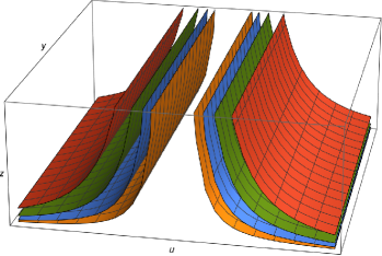
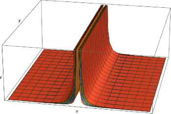
Figure 4: The “Mohawk:” the bending of the groups of M5 branes by intersecting M2 branes. The groups are separated and bent according to the value of $\frac{Q_{M2}}{Q_{M5}}$. At infinity, the M2 and M5 branes limit to coincident stacks, as depicted in the figure on the right. The two plots show the mohawk closer in and zoomed out, revealing the separation of the branes and their asymptotic convergence.

5 Final comments

Our primary interest in brane fractionation is to capture the twisted sectors of the CFT’s that arise on coincident stacks of two species of brane. The standard work-horse for CFT’s on brane intersections is the D1-D5 system in which the CFT has a well-understood, weak-coupling limit. Here we have focussed on M2-M5 intersections because the structure of the solutions on the internal manifold is simpler.

In the standard picture, the twisted sectors, and the majority of microstates, emerge from some form of fractionation leading to a “Higgs Branch.” In the D1-D5 system one gets $4N_{1}N_{5}$ scalars from the instanton moduli space of D1’s inside D5’s. For the M2-M5 system, these scalars come from the $4N_{2}N_{5}$ positions of the fractionated branes depicted in the first part of Fig. 5.

To capture this fractionation with supergravity, one has to fractionate the branes only partially, so that each “brane segment” still has a sufficiently large number of branes to produce a significant gravitational back-reaction. We also have to choose the compactification scale to be sufficiently large so that the supergravity approximation is valid.

In this paper we have shown that brane fractionation can happen at two qualitatively different levels. The first is the one we just described. However, we have shown that there is a second fractionation, depicted in Fig. 2 and the second part of Fig. 5, which occurs at each individual intersection. This fractionation preserves an AdS isometry, creating what we have called the M2-M5 mohawk. Since this second fractionation occurs within a single AdS₃, its holographic interpretation should be captured by the conformal field theory dual to a single brane intersection.

Consider one such intersection with $N_{2}$ M2 branes and $N_{5}$ M5 branes, and the “intersection CFT” that it creates. This can result in many different mohawk configurations that are characterized by all the possible sets of $\frac{N_{2,a}}{N_{5,a}}$ consistent with the total brane charges. We conjecture that each of these different mohawk configurations corresponds to a ground state of this CFT. It would be interesting to count how many such configurations exist for a total $N_{2}$ and $N_{5}$. This is given by the total number of ways one can write families of fractions of the type $\frac{N_{2,a}}{N_{5,a}}$ with $\sum_{a}N_{2,a}=N_{2}$ and $\sum_{a}N_{5,a}=N_{5}$. We leave the evaluation of this number and its large-$N$ growth to mathematics aficionados. More broadly, one would like to obtain a more complete understanding of the underlying CFT and its ground-state structure.

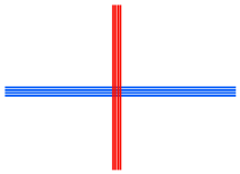
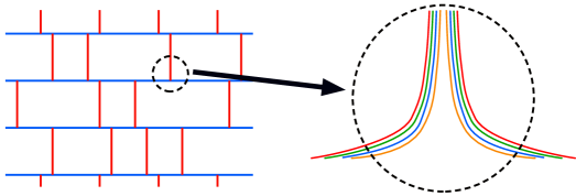
Figure 5: Brane fractionation. The first step shows “standard” brane fractionation in flat space. The second step shows “second-level” fractionation in a near-brane limit in which the back-reaction creates self-similar spikes whose scale invariance is transmogrified into an AdS₃ space. In the first step the moduli are the positions of each brane segment, while, in the second step, the position of each spike is controlled by the charge ratio in the spike.

The results presented here suggest a number of very interesting follow-up projects. First, following on from [9], it would be very interesting to add momentum waves to these mohawk solutions so as to obtain $\frac{1}{8}$-BPS microstate geometries. More specifically, the goal of studying supergravity solutions that describe fractionated branes is to see how supergravity can access the twisted sectors of the CFT. If one can add independent momentum waves to each and every intersection point, then one will obtain a coherent supergravity model of the fractionated black-hole microstructure. As it was originally envisaged [4, 19, 20, 8, 21, 9], this momentum partitioning was to be done at the “first level” of partitioning as depicted in the first part of Fig. 5. The challenge in this approach is that the intersecting brane system is governed by a non-linear system of equations. (Nevertheless, the equations governing the momentum excitations and related fluxes were shown to be linear in [9].)

The new opportunity presented by this work is the emergence of the second level of fractionation in a near-brane limit, depicted in the second part of Fig. 5. These solutions are simpler, the background is governed by linear equations, and the brane intersections are characterized via the geometry of a Riemann surface. These near-brane geometries and their fractionation will thus provide a simpler setting for the investigation of momentum partitioning at fractionated intersections.

While we believe our example in Section 3 is representative, it is, from the perspective of [1], only a small subset of a diverse family of solutions. In particular, there is the parameter, $\gamma$, that determines the representation of the underlying superalgebra, and there is also the option to consider more general Riemann surfaces with more general flux functions, $G$. Indeed, there is a discussion of “Lego pieces” in [1] that suggests that one might be able to plumb together more complicated brane intersections using multiply punctured Riemann surfaces.

In this paper, we took the Riemann surface to be the entire Poincaré half plane. Moreover, as noted in [8, 9], the residual supersymmetry also allows one to include additional M5-brane sources, usually denoted as M5’, that share $(t,y)$ but fill the spatial directions transverse to the original M2 and M5 branes. These directions are described by $v$ and the sphere $S^{\prime}{}^{3}$ in Section 2. We have excluded such M5’ sources. (This is why we chose all the sources in Section 3 to be in the region $G\to-i$.) Based on the analysis in [9], we also set the supersymmetry parameter, $\gamma$, to $1$.

All of this greatly limits the “Lego pieces” described in [1], and excluding M5’ brane sources places further limitations. It would be interesting to see if one can do something more general by freeing up the $\gamma$-parameter, and allowing a more general geometry for the common intersection of the branes. On the other hand, there has to be a price for taking the near-brane limit and getting an AdS factor in the geometry. As we have discussed in our example, the scaling of the AdS arises from the self-similarity of the bending of brane intersections. There must be a similar scale invariance in other brane intersections described by the results in [1], and, as we remarked in the Introduction, this will still limit the possibilities.

The near-brane limits of the intersecting M2-M5 system that can be incorporated as components of microstate geometries will therefore be a restricted sub-class of the families of solutions obtained in [1]. Nevertheless, we suspect that one can generalize beyond the example presented here, and even in this example we have seen that there is a rich structure to the “mohawk” that will prove invaluable to understanding momentum-carrying black-hole microstates.

Acknowledgements: We would like to thank Costas Bachas and Eric d’Hoker for interesting discussions. The work of IB and NPW was supported in part by the ERC Grant 787320 - QBH Structure. The work of IB was also supported in part by the ERC Grant 772408 - Stringlandscape and by grant NSF PHY-2309135 to the Kavli Institute for Theoretical Physics (KITP). The work of SC received funding under the Framework Program for Research and “Horizon 2020” innovation under the Marie Skłodowska-Curie grant agreement no 945298. This work was supported in part by the FACCTS Program at the University of Chicago. The work of DT was supported in part by the Onassis Foundation - Scholarship ID: F ZN 078-2/2023-2024 and by an educational grant from the A. G. Leventis Foundation. The work of NPW was also supported in part by the DOE grant DE-SC0011687.

Appendices

Appendix A Probe M5-branes

We demonstrated in the main text that the solutions in Section 3 correspond to a single stack of semi-infinite M2-branes ending on a single stack of M5 branes, which, as one gets closer to their intersection, separate into different M2-M5 spikes depending on the values of $\xi_{a}$ and $\zeta_{a}$. The AdS radius, $\mu$, sweeps the radial direction in the combined world-volume. In this Appendix, we would like to underline and elucidate our interpretation of the supergravity geometry by using probes that are M5 branes with an M2 spike. These probes have nontrivial M5 worldvolume fluxes. We expect that one can add such a “spiked” brane probe to the background determined by (3.2) and, because of (4.26), we anticipate that such probe branes will feel no force when located on the boundary of the Riemann surfaces at a $\xi$-position that scales linearly with the amount of M2 world-volume charge. We show that both of these expectations are correct.

Instead of working with the M5-brane action, which is rather complicated [22], we will reduce the M-theory background to a Type-IIA one and evaluate the action of a spiked D4 brane. We start with the metric and fluxes in (2.8) and use the Poincaré $AdS_{3}$ metric:

$$ds_{11}^{2} ~{}=~{}f_{1}^{2}\left(\frac{d\mu^{2}}{\mu^{2}}+\mu^{2}\left(-dt^{2}+dy^{2}\right)\right)~{}+~{}f_{2}^{2}\,ds_{S^{3}}^{2}~{}+~{}f_{3}^{2}\,ds_{{S^{\prime}}^{3}}^{2}~{}+~{}f_{4}^{2}|dw|^{2}\,,$$ (A.1)

$$C^{(3)} ~{}=~{}b_{1}\,\hat{e}^{012}~{}+~{}b_{2}\,\hat{e}^{345}~{}+~{}b_{3}\,\hat{e}^{678}\,,$$

where we have absorbed the overall $e^{2A}$ factor into the $f_{i}$’s, which are given by:

$$f_{1}^{6} =\frac{h^{2}W_{+}W_{-}}{64(G\overline{G}-1)^{2}}\,,\hskip 30.0ptf_{2}^{6}=\frac{h^{2}(G\overline{G}-1)W_{-}}{W_{+}^{2}}\,,$$ (A.2)

$$f_{3}^{6} =\frac{h^{2}(G\overline{G}-1)W_{+}}{W_{-}^{2}}\,,\hskip 20.0ptf_{4}^{6}=\frac{|\partial_{w}h|^{6}}{h^{4}}(G\overline{G}-1)W_{+}W_{-}\,.$$

In order to go to a Type IIA duality frame, we reduce the 11-dimensional solution along the $y$ direction. Using the usual relations between type IIA and 11-dimensional supergravity solutions

$$ds_{11}^{2} =e^{-\frac{2\phi}{3}}ds_{10}^{2}+e^{\frac{4\phi}{3}}(dx+C_{1})^{2}\,,$$ (A.3)

$$C_{3}^{\prime} =C_{3}+B_{2}\wedge dx\,,$$ (A.4)

where $x$ is the direction along which we reduce, we arrive at the following type IIA solution:

$$ds_{10}^{2} =-\mu^{3}f_{1}^{3}dt^{2}+\frac{f_{1}^{3}}{\mu}d\mu^{2}+\mu f_{1}f_{2}^{2}ds_{S^{3}}^{2}+\mu f_{1}f_{3}^{2}ds_{{S^{\prime}3}^{3}}^{2}+\mu f_{1}f_{4}^{2}|dw|^{2}\,,$$ (A.5)

$$C_{3} =b_{2}\,\hat{e}^{345}~{}+~{}b_{3}\,\hat{e}^{678}\,,\hskip 15.0ptB_{2}=-\mu b_{1}dt\wedge d\mu\,,\hskip 15.0pte^{2\phi}=\mu^{3}f_{1}^{3}\,.$$

We consider a probe M5-brane extending along $AdS_{3}\times S^{3}$ with world-volume M2 flux on it. We will take the worldvolume of the brane to be along the $AdS_{3}$ factor of the metric, since this is the only way for the probe to preserve the symmetries of the background. However, since we reduce along $y$ we will instead study a D4-brane with world-volume F1 flux along it. We will take the world-volume of the D4 to be parametrized by $(\eta_{0},\eta_{1},\eta_{2},\eta_{3},\eta_{4})$ with $(\eta_{0},\eta_{1})$ identified respectively with $t$ and $\mu$ and $(\eta_{2},\eta_{3},\eta_{4})$ identified with the coordinates on $S^{3}$. The induced metric on our probe brane is therefore:

$$d\tilde{s}_{5}^{2}=-\mu^{3}f_{1}^{3}dt^{2}+\frac{f_{1}^{3}}{\mu}d\mu^{2}+\mu f_{1}f_{2}^{2}ds_{S^{3}}^{2}$$ (A.6)

and the induced NS-NS and RR fields are

$$\tilde{B}_{2}=-\mu b_{1}dt\wedge d\mu\,,\quad\quad\tilde{C}_{3}=b_{2}\hat{e}^{345}\,.$$ (A.7)

In order to account for the F1 charge, we turn on a world-volume 2-form field of the form:

$$F_{2}~{}=~{}\mathcal{F}dt\wedge d\mu~{}=~{}(\partial_{t}A_{\mu}-\partial_{\mu}A_{0})\,dt\wedge d\mu\,,$$ (A.8)

where the gauge potential, $A$, and the Maxwell field, $\mathcal{F}$, are, in principle, functions of $\mu$ and the Riemann surface coordinates $(\xi,\rho)$.

It is then straightforward to compute the DBI and WZ actions:

$$S_{DBI} =-T_{4}\int\,d^{5}\eta e^{-\phi}\sqrt{-\det\left(\tilde{G}_{\alpha\beta}+F_{\alpha\beta}+\tilde{B}_{\alpha\beta}\right)}=-T_{4}\int dt\,dy\,d\Omega_{3}\,f_{2}^{3}\sqrt{\mu^{2}f_{1}^{6}-(\mathcal{F}-\mu b_{1})^{2}}\,,$$

$$S_{WZ} =-T_{4}\int\,e^{\tilde{B}_{2}+\tilde{F}_{2}}\wedge\oplus_{n}\tilde{C}_{n}=-T_{4}\int dt\,dy\,d\Omega_{3}\,(F-\mu b_{1})b_{2}-T_{4}\int\,\tilde{C}_{5}\,.$$ (A.9)

In order to determine $\tilde{C}_{5}$, we need to use the fact that:

$$F_{p} =dC_{p-1}\hskip 88.0pt\text{for }p<3\,,$$

$$F_{p} =dC_{p-1}+H_{3}\wedge C_{p-3}\hskip 25.0pt\text{for }p\geq 3\,,$$ (A.10)

$$F_{6} =\star F_{4}\,,\hskip 20.0ptF_{8}=\star F_{2}\,.$$

Employing these and noting that $C_{1}=0$ we arrive at

$$dC_{5}= \star\left(db_{2}\wedge\hat{e}^{345}\right)+\mu b_{3}db_{1}\wedge dt\wedge d\mu\wedge\hat{e}^{678}\,$$ (A.11)

$$\star\left(db_{3}\wedge\hat{e}^{678}\right)+\mu b_{2}db_{1}\wedge dt\wedge d\mu\wedge\hat{e}^{345}\,,$$

where $\star$ denotes the 10-dimensional Hodge star operator. The first term of the expression above gives a $C_{5}$ along the Riemann surface, $\Sigma$, and $dt\wedge d\mu\wedge\hat{e}^{678}$, while the second gives a $C_{5}$ along $\Sigma$ and $dt\wedge d\mu\wedge\hat{e}^{345}$. Since we only need the pullback of $C_{5}$ to the D4-brane probe world-volume, we only need the terms of the second line, which give the following contribution:

$$\mu\frac{f_{1}^{3}f_{2}^{3}}{f_{3}^{3}}\left(\partial_{\xi}b_{3}\,d\rho-\partial_{\rho}b_{3}\,d\xi\right)\wedge dt\wedge d\mu\wedge d\Omega_{3}+\mu b_{2}\left(\partial_{\xi}\,d\xi+\partial_{\rho}\,d\rho\right)\wedge dt\wedge d\mu\wedge d\Omega_{3}\,.$$ (A.12)

Integrating this expression is quite complicated and since we will eventually only care about the derivative of $C_{5}$ along the $\xi$ direction we will leave (A.12) as it is.

The conjugate momentum to $\mathcal{F}$ captures the number of F1 strings (or equivalently M2 branes) that form the spike that ends to the D4 (or M5) branes:

$$\Pi=\frac{\partial\mathcal{L}}{\partial{(\partial_{t}A_{\mu})}}=\left(-b_{2}+\frac{f_{2}^{3}\left(\mathcal{F}-\mu b_{1}\right)}{\sqrt{\mu^{2}f_{1}^{6}-\left(\mathcal{F}-\mu b_{1}\right)^{2}}}\right)\,.$$ (A.13)

The Hamiltonian density is now easily obtained:

$$\mathcal{H}~{}=~{}\Pi\,(\partial_{t}A_{\mu})~{}-~{}\mathcal{L}~{}=~{}-\mu b_{1}b_{2}+f_{2}^{3}\frac{\mu b_{1}\left(\mathcal{F}-\mu b_{1}\right)+\mu^{2}f_{1}^{6}}{\sqrt{\mu^{2}f_{1}^{6}-\left(\mathcal{F}-\mu b_{1}\right)^{2}}}+\tilde{C}_{5}\,.$$ (A.14)

The equation of motion obtained by varying the action, (A.9), with respect to $A_{0}$, yields $\partial_{\mu}\Pi=0$. This is satisfied if one chooses $\mathcal{F}=\mu F(\rho,\xi)$. Solving for $F$ in (A.13), we obtain

$$F~{}=~{}b_{1}\pm\frac{f_{1}^{3}|b_{2}+\Pi|^{2}}{\sqrt{f_{2}^{6}+\left(b_{2}+\Pi\right)^{2}}}\,,$$ (A.15)

which we use to express the Hamiltonian only in terms of $\Pi$:

$$\mathcal{H}/\mu~{}=~{}-b_{1}b_{2}+f_{1}^{3}\sqrt{f_{2}^{6}+\left(b_{2}+\Pi\right)^{2}}\pm b_{1}|b_{2}+\Pi|+\tilde{C}_{5}\,.$$ (A.16)

This Hamiltonian is a function of the Riemann-surface coordinates $(\xi,\rho)$, but we are interested in putting probes on $\partial\Sigma$ and so we will take its $\rho\rightarrow 0$ limit. We will then interpret it as a potential in the $\xi$ direction and find its minima for a given value of $\Pi$ in a given background geometry. The expression in (A.16) has two possible forms depending on which solution of $F$ we choose in (A.15) and on whether $b_{2}+\Pi$ is less or greater than zero. This choice depends on whether we add M2 or anti-M2 charge to the M5-world-volume. For the particular example we will study here we will take the minus solution and assume that $b_{2}+\Pi<0$ to arrive at

$$\mathcal{H}/\mu=\Pi\,b_{1}+f_{1}^{3}\sqrt{f_{2}^{6}+\left(b_{2}+\Pi\right)^{2}}+\tilde{C}_{5}\,.$$ (A.17)

Moreover, we will express $b_{i}$ in terms of $\hat{b}_{i}$ (see the discussion below (4.4)) and we will factor out $\frac{\nu_{3}\sigma}{c_{1}^{3}c_{2}^{3}}$ to simplify our computation. Keeping only the $d\xi$ terms in (A.12) and noting that $c_{1}c_{2}c_{3}f_{1}f_{2}f_{3}=\sigma h$ we arrive at:

$$\partial_{\xi}\mathcal{H}=\frac{\nu_{3}\sigma}{c_{1}^{3}c_{2}^{3}}\partial_{\xi}\hat{\mathcal{H}}=\frac{1}{8}\left(8\,\partial_{\xi}\left(f_{1}^{3}\sqrt{f_{2}^{6}+(\Pi-\hat{b}_{2})^{2}}\right)+(\Pi-\hat{b}_{2})\,\partial_{\xi}\hat{b}_{1}-\frac{h^{3}}{f_{3}^{6}}\partial_{\rho}\hat{b}_{3}\right)\,.$$ (A.18)

In Fig. 6 we depict the function $\partial_{\xi}\mathcal{H}$ for various values of $\Pi$ and for solutions with two and three poles in $G$. By explicitly computing the zeros of this function we observe that they follow a linear growth in $\Pi$. In particular, we find that

$$\xi_{0}\simeq-\frac{1}{4}\Pi+c\,,$$ (A.19)

where $\xi_{0}$ denotes the minimum of $\mathcal{H}$ and $c$ is a constant that depends on our gauge choices and the parameters of the particular solution we are probing.

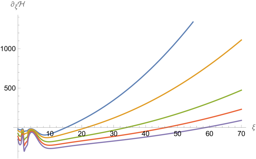
(a) Two-pole solution

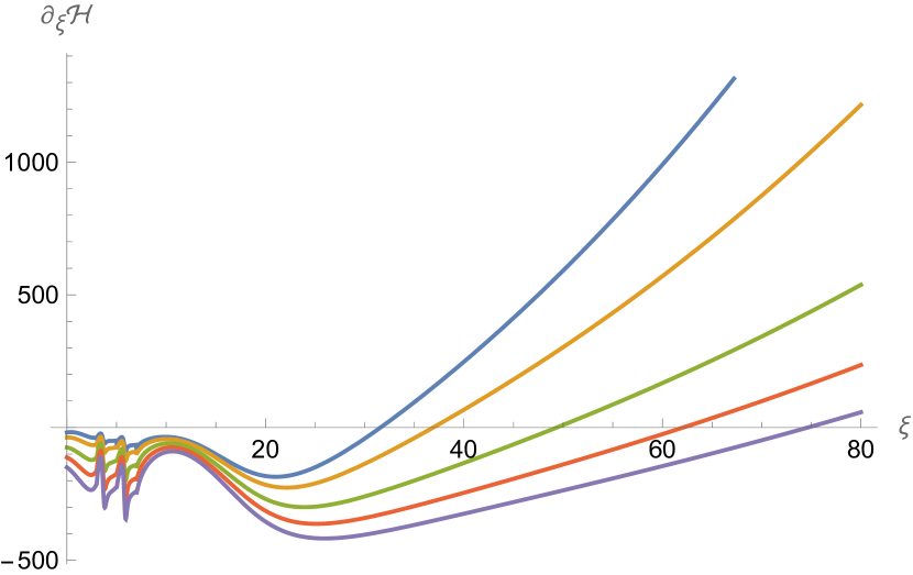
(b) Three-pole solution

Figure 6: Solution with two poles in $G$ with parameters $(\xi_{1},\xi_{2},\zeta_{1},\zeta_{2},\hat{b}_{0}^{2})=(1,3,1,1,4)$ (a) and solution with three poles in $G$ with parameters $(\xi_{1},\xi_{2},\xi_{3},\zeta_{1},\zeta_{2},\zeta_{3},\hat{b}_{0}^{2})=(3,5,7,1,2,3,12)$ (b). In both graphs $\Pi$ takes the values $(-25,-50,-100,-150,-200)$ from left to right.

The relation, (A.19), is expected since $\Pi$ roughly corresponds to $\sim Q_{M2}/Q_{M5}$ and if we think of our probe as another spike in the solution we are examining, we expect from (4.26) that its position on the $\xi$ axis will scale with $Q_{M2}$ in the following way:

$$\frac{Q_{M2,0}}{Q_{M5,0}}\sim-\frac{16\zeta_{0}}{4\zeta_{0}}\xi_{0}\quad\Rightarrow\quad\xi_{0}\sim-\frac{1}{4}\Pi\,.$$ (A.20)

For the values of $\Pi$ and solution parameters we used in Fig. 6 there are only minima to the right of the background spikes. However, for smaller values of $\Pi$ one can generally find a minimum also to the left of the spikes, and for sufficient separation between the location of the various poles it is also possible to find a minimum in between them. We therefore find that the equilibrium positions of our probes match precisely with the supergravity solution and our interpretation of it.

References

- [1] C. Bachas, E. D’Hoker, J. Estes, and D. Krym, “M-theory Solutions Invariant under ,” Fortsch. Phys. 62 (2014) 207–254, arXiv:1312.5477 [hep-th].
- [2] I. Bena, N. Ceplak, S. Hampton, Y. Li, D. Toulikas, and N. P. Warner, “Resolving black-hole microstructure with new momentum carriers,” JHEP 10 (2022) 033, arXiv:2202.08844 [hep-th].
- [3] I. Bena, E. J. Martinec, S. D. Mathur, and N. P. Warner, “Snowmass White Paper: Micro- and Macro-Structure of Black Holes,” arXiv:2203.04981 [hep-th].
- [4] I. Bena, E. J. Martinec, S. D. Mathur, and N. P. Warner, “Fuzzballs and Microstate Geometries: Black-Hole Structure in String Theory,” arXiv:2204.13113 [hep-th].
- [5] J. de Boer, A. Pasquinucci, and K. Skenderis, “AdS / CFT dualities involving large 2-D N=4 superconformal symmetry,” Adv. Theor. Math. Phys. 3 (1999) 577–614, arXiv:hep-th/9904073 [hep-th].
- [6] O. Lunin, “Strings ending on branes from supergravity,” JHEP 09 (2007) 093, arXiv:0706.3396 [hep-th].
- [7] O. Lunin, “Brane webs and 1/4-BPS geometries,” JHEP 0809 (2008) 028, arXiv:0802.0735 [hep-th].
- [8] I. Bena, A. Houppe, D. Toulikas, and N. P. Warner, “Maze Topiary in Supergravity,” arXiv:2312.02286 [hep-th].
- [9] I. Bena, R. Dulac, A. Houppe, D. Toulikas, and N. P. Warner, “Waves on Mazes,” arXiv:2404.14477 [hep-th].
- [10] E. D’Hoker, J. Estes, M. Gutperle, and D. Krym, “Exact Half-BPS Flux Solutions in M-theory. I: Local Solutions,” JHEP 08 (2008) 028, arXiv:0806.0605 [hep-th].
- [11] E. D’Hoker, J. Estes, M. Gutperle, and D. Krym, “Exact Half-BPS Flux Solutions in M-theory II: Global solutions asymptotic to AdS(7) x S**4,” JHEP 12 (2008) 044, arXiv:0810.4647 [hep-th].
- [12] E. D’Hoker, J. Estes, M. Gutperle, D. Krym, and P. Sorba, “Half-BPS supergravity solutions and superalgebras,” JHEP 12 (2008) 047, arXiv:0810.1484 [hep-th].
- [13] E. D’Hoker, J. Estes, M. Gutperle, and D. Krym, “Janus solutions in M-theory,” JHEP 06 (2009) 018, arXiv:0904.3313 [hep-th].
- [14] E. D’Hoker, J. Estes, M. Gutperle, and D. Krym, “Exact Half-BPS Flux Solutions in M-theory III: Existence and rigidity of global solutions asymptotic to AdS(4) x S**7,” JHEP 09 (2009) 067, arXiv:0906.0596 [hep-th].
- [15] N. Bobev, K. Pilch, and N. P. Warner, “Supersymmetric Janus Solutions in Four Dimensions,” JHEP 06 (2014) 058, arXiv:1311.4883 [hep-th].
- [16] C. G. Callan and J. M. Maldacena, “Brane death and dynamics from the Born-Infeld action,” Nucl. Phys. B 513 (1998) 198–212, arXiv:hep-th/9708147.
- [17] N. R. Constable, R. C. Myers, and O. Tafjord, “The Noncommutative bion core,” Phys. Rev. D 61 (2000) 106009, arXiv:hep-th/9911136.
- [18] O. Lunin, “1/2-BPS states in M theory and defects in the dual CFTs,” JHEP 10 (2007) 014, arXiv:0704.3442 [hep-th].
- [19] I. Bena, S. D. Hampton, A. Houppe, Y. Li, and D. Toulikas, “The (amazing) super-maze,” JHEP 03 (2023) 237, arXiv:2211.14326 [hep-th].
- [20] I. Bena, N. Čeplak, S. D. Hampton, A. Houppe, D. Toulikas, and N. P. Warner, “Themelia: the irreducible microstructure of black holes,” arXiv:2212.06158 [hep-th].
- [21] I. Bena and R. Dulac, “Born-Infeld supermaze waves,” JHEP 05 (2024) 063, arXiv:2312.13447 [hep-th].
- [22] I. A. Bandos, K. Lechner, A. Nurmagambetov, P. Pasti, D. P. Sorokin, and M. Tonin, “Covariant action for the superfive-brane of M theory,” Phys. Rev. Lett. 78 (1997) 4332–4334, arXiv:hep-th/9701149.