Interpretation of recently discovered single bottom baryons in the relativistic flux tube model

Abstract

Following recent experimental progress in the study of bottom baryons, we systematically calculate the mass spectra of $\Lambda_{b}$, $\Xi_{b}$, $\Sigma_{b}$, $\Xi_{b}^{{}^{\prime}}$, and $\Omega_{b}$ baryons with a quark-diquark picture in the framework of a relativistic flux tube model with spin-dependent interactions in the j-j coupling scheme. Furthermore, we calculate the strong decay width of bottom baryons decaying into a bottom baryon and a light pseudoscalar meson. A good agreement is found between the calculated masses and the experimentally available masses of singly bottom baryons. By analysing both mass spectra and strong decay widths, we interpret $\Sigma_{b}(6097)$ as a $1P(3/2^{-})$ state and $\Xi_{b}(6100)$ as a $1P(1/2^{-})$ state of $\Xi_{b}$ baryon. The $\Xi_{b}(6227)$ is identified to be an orbital excitation $1P$ of the $\Xi_{b}^{{}^{\prime}}$ baryon with $J^{P}=3/2^{-}$. Further, we determine $\Xi_{b}(6327)$ and $\Xi_{b}(6333)$ as a $1P(3/2^{-})$ state and $1P(5/2^{-})$ state, respectively, of $\Xi_{b}^{{}^{\prime}}$ baryon. From the obtained mass spectra, we construct the Regge trajectories in the $(J,M^{2})$ plane, which are found to be essentially linear, parallel, and equidistant. Our predictions for higher orbital and radial excited states can help experimentalists identify missing excited states of singly bottom baryons.

I INTRODUCTION

The discovery of a new hadron always comes up with a hint for us to better understand how quarks interact with each other in the hadronic system. Within the hadronic family, singly heavy baryons have an important position, as both chiral symmetry and heavy quark symmetry play a significant role in their dynamics. A thorough investigation of the observed singly heavy baryon can help us improve our understanding of the nature of the strong interaction in the domain of quark confinement. Experiments have observed more than 40 states of singly charmed baryons so far. However, searching for the single bottom baryon states is a difficult challenge for experimentalists since more energy and beam luminosity are required for their production. Furthermore, due to their short lifetime, they are extremely difficult to detect. Fig. 1 shows the experimental progress in discovering the singly bottom baryon states.

Figure 1: The experimentally observed states of singly bottom baryons

The first experimental observation of a singly bottom baryon, named $\Lambda_{b}(5620)^{0}$, was achieved in 1981 by CERN R415 [1]. After 14 years of this observation, in 1995, DELPHI announced the discovery of the first strange bottom baryons, $\Xi_{b}^{0}$ and $\Xi_{b}^{-}$ [2]. Then, $\Sigma_{b}^{\pm}$ and $\Sigma_{b}^{*\pm}$, were reported by the CDF experiment in 2007, long after the previous discovery [3]. In the following year, the first doubly strange bottom baryon, $\Omega_{b}^{-}$, was also observed by the D0 detector at the Fermilab Tevatron Collider [4].

Then, in the following years, especially with the start of LHCb Run 1, in 2011, many bottom baryons were expected to be observed. In 2012, CMS collaboration came up with the observation of $\Xi_{b}(5945)^{0}$ state [5]. In the same year, two narrow P-wave $\Lambda_{b}^{0}$ baryons, denoted as $\Lambda_{b}(5912)^{0}$ and $\Lambda_{b}(5920)^{0}$, were also discovered by the LHCb Collaboration [6], which was later confirmed by the CDF Collaboration [7]. In 2015, LHCb reported the ground state of $\Xi_{b}^{\prime}$ baryon, denoted as $\Xi_{b}^{{}^{\prime}}(5935)^{-}$, and the $\Xi_{b}(5955)^{-}$ state    [8] by analysing the data of run 1. In 2016, the isospin partner of $\Xi_{b}(5955)^{-}$, which is denoted a $\Xi_{b}(5945)^{0}$, was confirmed by LHCb with more precise measurement of mass [9].

At that point, many states were about to be identified as LHCb had taken collision data from run 2 in the period of 2015–2018. In 2018, they announced the discovery of $\Xi_{b}(6227)^{-}$ state [10] and two orbital excited states of $\Sigma_{b}$ baryon, $\Sigma_{b}(6097)^{+}$ and $\Sigma_{b}(6097)^{-}$ [11]. In 2019, they again reported two D-wave $\Lambda_{b}^{0}$ candidates, $\Lambda_{b}(6146)^{0}$ and $\Lambda_{b}(6152)^{0}$ [12]. The first observation of the four excited states of $\Omega_{b}$ baryon, named $\Omega_{b}(6316)^{-}$, $\Omega_{b}(6330)^{-}$, $\Omega_{b}(6340)^{-}$, and $\Omega_{b}(6350)^{-}$, was also announced by LHCb in 2020 [13]. Later in that year, they again observed $\Lambda_{b}(6070)^{0}$ state [14], which was subsequently confirmed by the CMS [15] experiment.

In 2021, the isospin partner of $\Xi_{b}(6227)^{-}$, named $\Xi_{b}(6227)^{0}$, is reported by LHCb [16]. In the same year, the CMS collaboration came up with the observation of $\Xi_{b}(6100)^{-}$ state [17]. Later in the same year, two new $\Xi_{b}$ states, namely $\Xi_{b}(6327)^{0}$ and $\Xi_{b}(6333)^{0}$, are reported by the LHCb collaboration [18].

These experimental discoveries have motivated a variety of theoretical studies. The systematic study of the mass spectra of all singly bottom baryons, up to high radial and orbital excited states, was first performed by Ebert et. al. [19]. The recent theoretical study on the mass spectra of singly bottom baryons includes the work by Garcia-Tecocoatzi et. al. in which the Hamiltonian model is used with a three-quark and a quark-diquark picture of baryons [20]. The authors in ref. [21, 22] study the mass spectra of both strange and non-strange singly bottom baryons using the relativistic quark model. In addition to these recent studies, it has been studied by the non-relativistic constituent quark model [23, 24, 25, 26], the hyper-central constituent quark model [27, 28, 29], the Regge trajectory model [30], the QCD spectral sum rules [31, 32], the QCD bag model [33], the QCD sum rule [34, 35], the lattice QCD [36, 37]. The more theoretical studies with more references can be found in review articles [38, 39, 40, 41].

Although there are multiple theoretical and experimental approaches, very few states of single bottom baryons have been established. The spin-parity of $\Sigma_{b}(6097)$, $\Xi_{b}(6100)$ $\Xi_{b}(6227)$, $\Xi_{b}(6327)$, $\Xi_{b}(6333)$, $\Omega_{b}(6316)$, $\Omega_{b}(6330)$, $\Omega_{b}(6340)$, and $\Omega_{b}(6350)$ are still unknown. Assigning spin parity is crucial as it aids in determining their experimental properties. As various theoretical approaches yield different predictions about the spin parity for these states, it is important to do more theoretical investigations and compare them with experimental data in order to identify them. This motivates us to systematically examine the mass spectra of single-bottom baryons.

In Ref.[42], the authors have calculated the mass spectrum of $\Lambda_{c/b}$ and $\Xi_{c/b}$ baryons utilising a linear Regge relation derived in a relativistic flux tube model. However, they opt out of investigating other singly heavy baryonic systems ($\Sigma_{c/b}$, $\Xi_{c/b}^{{}^{\prime}}$, and $\Omega_{c/b}$ baryons) containing vector diquarks due to the intricate nature of spin-dependent interactions. In our previous work [43, 44], we conducted calculations of the mass spectra for all singly charmed baryons using this linear Regge relation developed from the relativistic flux tube model that incorporates the spin-dependent interactions in the j-j coupling scheme. The aim of the present article is to extend this model to calculate the single-bottom baryon mass spectra. This will help us to assign possible spin parity to the experimentally detected states and to predict the masses of unobserved excited states, which can provide some significant information for future experiments.

The structure of the paper is as follows: In Section II, we describe the details of the relativistic flux tube model for singly bottom baryons, as well as the methodology employed to calculate their mass spectra. In section III, we present the formulation to compute the strong decay widths. In Section IV, we discuss the results  and compare them with other theoretical estimations. In addition, we discuss  our assignment to the available experimental states  by examining their mass spectrum and decay widths. In Section V, we present our conclusion.

II MASS SPECTRUM

II.1 Singly bottom baryons in RFT model

The singly bottom baryons can be seen as a bound system of a bottom quark ($b$) and two light quarks ($qq$, where q represents $u$, $d$, or $s$ quarks). There are different types of interactions in the system, such as quark-quark interaction, quark-gluon interaction, and gluon-gluon interaction, that make it a complex system to study.

To simplify this problem a bit, the heavy quark symmetry suggests that the coupling between two light quarks is stronger than the coupling between a bottom quark and a light quark [45]. It follows that two light quarks might couple first to form a diquark, which could then couple with a bottom quark, resulting in singly bottom baryonic states. In this way, we can reduce the three-body problem ($bqq$) into a two-body problem by taking a heavy-bottom-quark-light-diquark picture of singy bottom baryons. In this picture, the diquark is assumed to stay in ground state i.e. the relative motion between two light quarks are restricted and the two light quarks excite together as a pair relative to the bottom quark. This mode of excitation is called $\lambda$-mode of excitation. In contrast, within the three-body picture of the baryon, there also exists the $\rho$-mode of excitation, which involves the relative motion between the two light quarks. In quark-diquark baryon picture, as the $\rho$-mode of excitation is absent, the number of possible states decreases significantly compare to that in three-body picture of the baryon [20, 46]. As the $\rho$-mode excitations of singly bottom baryons are not observed experimentally, it supports the idea that singly bottom baryons are better described by a quark-diquark picture [42]. Although $\rho$-mode excitations may not be observed for various reasons, particularly their higher energy levels, large decay widths, and suppressed transitions, this suggests that further experimental and theoretical studies are required to understand the structure of singly bottom baryons.

For simplicity, we assume the quark-diquark baryon model in our investigation, which is also supported by a number of theoretical frameworks[47, 48, 49]. In this picture, the diquark and bottom quark are confined inside the baryon through strong interaction carried by gluons. One effective way to capture some essential features of confinement is the relativistic flux tube model. In this model, the confining interaction between bottom quark and diquark is carried out by a thin, string-like object called a flux tube. A gluonic field between the bottom quark and the diquark is restricted to a flux tube having a constant tension ($T$). The light quarks within diquark are assumed to stay in their ground state. The effect of interaction between two light quarks within diquark is included in the mass of diquark. The whole system of the bottom quark, diquark, and flux tube rotates around its centre of mass, giving rise to different quantum states of the system. A linear Regge relation between mass ($\bar{M}$) and angular momentum quantum number ($L$) of a singly heavy baryonic system can be obtained using this model as [42, 43]

$$(\bar{M}-m_{b})^{2}=\frac{\sigma}{2}L+(m_{\mathcal{D}}+m_{b}v_{2}^{2}),$$ (1)

Here, $\sigma=2\pi T$. As the diquark in its ground state with current mass $m_{1}$ and the bottom quark with current quark mass $m_{2}$ rotate with speeds $v_{1}$ and $v_{2}$, respectively, their effective masses are $m_{\mathcal{D}}=m_{1}/\sqrt{1-{v_{1}^{2}}}$ and $m_{b}=m_{2}/\sqrt{1-{v_{2}^{2}}}$, respectively. The light diquark is assumed to rotate with ultra-relativistic speed, which leads to the assumption that it’s speed, $v_{1}=1$.

The distance between the bottom quark and the diquark in this model is given as [42]

$$r=(v_{1}+v_{2})\sqrt{\frac{8L}{\sigma}}.$$ (2)

For a two-body picture of a heavy-light hadronic system, the quantum solution of the RFT model predicts that the Regge trajectories in the $(L,(\bar{M}-m_{b})^{2})$ plane, for different radial excitations, are parallel and equidistant to each other [50, 51, 52]. This study leads us to modify our semi-classical relations (1) and (2) by replacing $L$ with $\lambda n_{r}+L$ (here, $n_{r}=n-1$, whereas n is the principle quantum number having values 1, 2, 3, etc., representing different radial excitations) to get a parallel and equidistant radial Regge trajectories in the $(L,(\bar{M}-m_{b})^{2})$ plane. The modified relationships are

$$(\bar{M}-m_{b})^{2}=\frac{\sigma}{2}[\lambda n_{r}+L]+(m_{\mathcal{D}}+m_{b}v_{2}^{2}),$$ (3)

and

$$r=(v_{1}+v_{2})\sqrt{\frac{8[\lambda n_{r}+L]}{\sigma}}.$$ (4)

Here, $\lambda$ is a parameter of our model that defines the vertical distance between the Regge trajectories (corresponding to principle quantum numbers $n=1,2,3,..$) in the $(L,(\bar{M}-m_{b})^{2})$ plane.

II.2 Spin-dependent splittings and singly bottom baryon states

Since the RFT model assumes the quarks to be spinless particles, we must now account for the contribution to mass from spin-dependent interactions from QCD motivated quark potential model, as

$$\Delta{M}=H_{so}+H_{t}+H_{ss}.$$ (5)

Here, $H_{so}$ is a spin-orbit interaction term, given as [53]

$$\begin{split}H_{so}&=[(\frac{2\alpha}{3r^{3}}-\frac{b^{\prime}}{2r})\frac{1}{m_{\mathcal{D}}^{2}}+\frac{4\alpha}{3r^{3}}\frac{1}{m_{\mathcal{D}}m_{b}}]\mathbf{L}\cdot\mathbf{S_{\mathcal{D}}}\\ &\hskip 8.5359pt+[(\frac{2\alpha}{3r^{3}}-\frac{b^{\prime}}{2r})\frac{1}{m_{b}^{2}}+\frac{4\alpha}{3r^{3}}\frac{1}{m_{\mathcal{D}}m_{b}}]\mathbf{L}\cdot\mathbf{S_{b}}.\\ \end{split}$$ (6)

It comes from the short-range one-gluon exchange contribution and the long-range Thomas-precession term. The spin of bottom quark and diquark is represented by $\mathbf{S_{b}}$ and $\mathbf{S_{\mathcal{D}}}$, respectively. $\mathbf{L}$ denotes the orbital angular momentum of the system. Further, the tensor interaction term,

$$\begin{split}H_{t}&=\frac{4\alpha}{3r^{3}}\frac{1}{m_{\mathcal{D}}m_{b}}[\frac{3(\mathbf{S_{\mathcal{D}}}\cdot\mathbf{r})(\mathbf{S_{b}}\cdot\mathbf{r})}{r^{2}}-\mathbf{S_{\mathcal{D}}}\cdot\mathbf{S_{b}}].\\ \end{split}$$ (7)

results from magnetic-dipole-magnetic-dipole color hyperfine interaction. For simplicity we define, $\mathbf{\hat{B}}$=$3(\mathbf{S_{\mathcal{D}}}\cdot\mathbf{r})(\mathbf{S_{b}}\cdot\mathbf{r})/r^{2}-\mathbf{S_{\mathcal{D}}}\cdot\mathbf{S_{b}}$. Lastly, the spin-spin contact hyperfine interaction is given as

$$\begin{split}H_{ss}&=\frac{32\alpha\sigma_{0}^{3}}{9\sqrt{\pi}m_{\mathcal{D}}m_{b}}e^{-\sigma_{0}^{2}r^{2}}\mathbf{S_{\mathcal{D}}}\cdot\mathbf{S_{b}}.\\ \end{split}$$ (8)

We can determine the parameters $b^{\prime}$ and $\sigma_{0}$ using experimental data. Due to these spin-dependent interactions ($\Delta M$), the states with mass $\bar{M}$ will split into different states having mass $\bar{M}+\Delta M$.

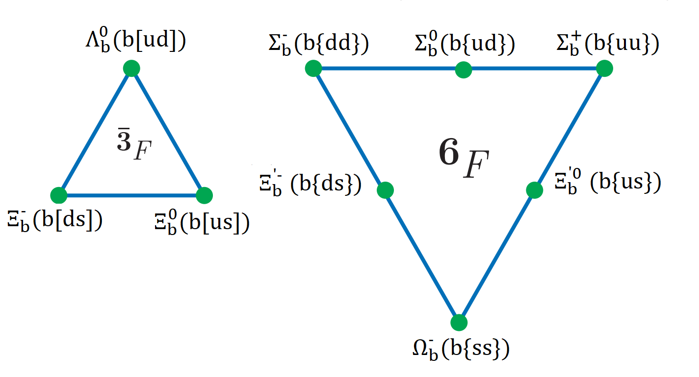
Figure 2: SU(3) flavor multiplets of singly bottom baryons. Anti-triplet($\bar{3}_{F}$) consist of $\Lambda_{b}$ and $\Xi_{b}$ baryons, while sextet($6_{F}$) consist of $\Sigma_{b}$, $\Xi_{b}^{{}^{\prime}}$, and $\Omega_{b}$ baryons.

If $SU_{F}(3)$ symmetry is considered for light quarks (u, d, and s), Pauli’s exclusion principle states that the total wavefunction of a diquark is antisymmetric. The total wave function of diquark consists of a product of its space-, color-, flavor-, and spin-wave functions. As two light quarks are in their ground state, the space wave function of a diquark is symmetric. The color wave function of a diquark is always antisymmetric. These conditions restrict the product of the flavor- and spin-wave functions of diquark to being symmetric. As shown in Fig.2, the SU(3) flavor symmetry of light quarks arranges the singly bottom baryons into two groups: the first is antitriplet ($\bar{3}_{F}$) with antisymmetric flavor wave function of light quarks, and the second is sextet ($6_{F}$) with symmetric flavor wave function of light quarks. To make the product of the flavor- and spin-wave functions of diquarks symmetric, diquarks belonging to the antitriplet and sextet flavor structures have to be spin-antisymmetric and spin-symmetric, respectively. This implies that the spin of a diquark present in $\Lambda_{b}$ and $\Xi_{b}$ baryons is $S_{\mathcal{D}}=0$, while that in $\Sigma_{b}$, $\Xi_{b}^{{}^{\prime}}$, and $\Omega_{b}$ baryons is $S_{\mathcal{D}}=1$. We represent scalar diquarks with $S_{\mathcal{D}}=0$ by $[qq]$, while vector diquarks with $S_{\mathcal{D}}=1$ by $\{qq\}$.

For $\Lambda_{b}$ and $\Xi_{b}$ baryons, the spin-depentent interactions are simple as $S_{\mathcal{D}}=0$. $\mathbf{S_{b}}$ directly couple with  $\mathbf{L}$ to give  $\mathbf{J}=\mathbf{L}+\mathbf{S_{b}}$. Squaring this, we obtain the expectation value of $\mathbf{L}\cdot\mathbf{S_{b}}$ as

$$\langle\mathbf{L}\cdot\mathbf{S_{b}}\rangle=\frac{1}{2}[J(J+1)-L(L+1)-S_{b}(S_{b}+1)].$$ (9)

In spin-dependent interactions, only a term proportional to $\mathbf{L}\cdot\mathbf{S_{b}}$ in spin-orbit interaction ($H_{so}$) survives. This term splits the state with given values of $L$ into two different states having $J=L\pm 1/2$ as listed in Tables 2 and 3.

For $\Sigma_{b}$, $\Xi_{b}^{{}^{\prime}}$, and $\Omega_{b}$ baryons, $\mathbf{S_{\mathcal{D}}}$ can couple with $\mathbf{S_{b}}$ and $\mathbf{L}$ in two ways. One possibility is that $\mathbf{S_{\mathcal{D}}}$ first couple with $\mathbf{S_{b}}$ to the total spin $\mathbf{S}=\mathbf{S_{\mathcal{D}}}+\mathbf{S_{b}}$, which subsequently couple with $\mathbf{L}$ giving total angular momentum $\mathbf{J}=\mathbf{L}+\mathbf{S}$. This way is called the  $L-S$  coupling scheme. The other way is that $\mathbf{S_{\mathcal{D}}}$ first couple with $\mathbf{L}$ to give the total angular momentum of diquark $\mathbf{j}=\mathbf{S_{\mathcal{D}}}+\mathbf{L}$, and then $\mathbf{j}$ couple with $\mathbf{S_{b}}$ to give $\mathbf{J}=\mathbf{j}+\mathbf{S_{b}}$. This scheme is known as the $j-j$ coupling scheme. The $j-j$ coupling scheme is preferred for singly bottom baryons due to their adherence to heavy quark symmetry. As a result of these couplings, the state with orbital angular momentum $L$ split into different states (as listed in Table 1, 4-6) defined by $j$ and $J$, where $j$ is diquark’s angular momentum quantum number and $J$ is the total angular momentum quantum number of the given state. Accordingly, we calculate the expectation values of $\mathbf{L}\cdot\mathbf{S_{\mathcal{D}}}$, $\mathbf{L}\cdot\mathbf{S_{b}}$, $\mathbf{S_{\mathcal{D}}}\cdot\mathbf{S_{b}}$, and $\mathbf{\hat{B}}$ in the $j-j$ coupling scheme and list them in Table 1. The computation of expectation values for these operators for $S$-wave, $P$-wave, and $D$-wave is presented in our previous work [43], and that for $F$-wave and $G$-wave is given in Appendix.

II.3 Determination of parameters

This section lists the values of parameters for readers’ convenience. The parameters involved in this theoretical model are $m_{b}$, $m_{\mathcal{D}}$, $v_{2}$, $\sigma$, $\lambda$, $\alpha$, $b^{\prime}$, and $\sigma_{0}$. Some of these parameters have already been extracted in our previous work [43] using experimentally available states of singly charmed baryons. The masses of diquarks ($m_{\mathcal{D}}$), with specific spin and quark combination ($[qq]$ or $\{qq\}$), were determined to be $m_{\mathcal{D}[u,d]}=0.503$ GeV, $m_{\mathcal{D}[d,s]}=0.687$ GeV, $m_{\mathcal{D}\{u,u\}}=0.714$ GeV, $m_{\mathcal{D}\{d,s\}}=0.841$ GeV, and $m_{\mathcal{D}\{s,s\}}=0.959$ GeV. Parameters involved in spin-dependent relations were calculated to be $\alpha$=0.426, $b^{\prime}$=-0.076 GeV², and $\sigma_{0}$=0.373248 GeV. The calculated value of $\lambda$ for $\Lambda_{b}$ and $\Xi_{b}$ baryons was 1.565, and that for $\Sigma_{b}$, $\Xi_{b}^{{}^{\prime}}$, and $\Omega_{b}$ baryons was 1.295. We adopt these previously extracted parameters to calculate the mass spectra of single-bottom baryons so that consistency is maintained in the model.

Additionally, we use the current quark mass of the bottom quark ($m_{2}=4.18$ GeV [54]) and the experimental mass of the ground state ($|1S,1/2^{+}\rangle$) of the $\Lambda_{b}$ baryon to get $m_{b}=4.499$ GeV and $v_{2}=0.37$. We calculate the spin average mass of the $1P$-wave for the $\Lambda_{b}$ baryon from the experimentally available masses of $\Lambda_{b}(5912)^{0}$ and $\Lambda_{b}(5920)^{0}$ states to extract $\sigma_{\Lambda_{b}}=1.512$ GeV². However, for other singly bottom baryons, the states belonging to the $1P$-wave are yet to be identified, which restricts us from directly extracting $\sigma$ from experimental data. Within the singly bottom baryonic family, all systems have the same heavy component, which is a bottom quark, but the mass of the light diquark varies due to different quark combinations and its spin (0 or 1). Consequently, the string tension of these systems could be a function of the diquark’s mass. In our previous work, for the singly charmed baryonic family, the string tension was assumed to be proportional to the $q^{th}$ power of the mass of diquark, i.e.

$$\sigma\propto m_{\mathcal{D}}^{q}.$$ (10)

We were able to describe the experimentally observed excited states of singly charmed baryons based on this assumption. The value of $q$ was determined to be 0.661. Inspired by this, we assume that relation [10] can also be applied to the singly bottom baryonic family. The ratio of $\sigma$ for $\Xi_{b}$ baryon and that for $\Lambda_{b}$ baryon,

$$\frac{\sigma_{\Xi_{b}}}{\sigma_{\Lambda_{b}}}=\left(\frac{m_{\mathcal{D}[d,s]}}{m_{\mathcal{D}[u,d]}}\right)^{q},$$ (11)

allow us to find $\sigma_{\Xi_{b}}=1.857$ GeV². Similarly, we obtain $\sigma_{\Sigma_{b}}=1.904$ GeV², $\sigma_{\Xi_{b}^{{}^{\prime}}}=2.122$ GeV², and $\sigma_{\Omega_{b}}=2.315$ GeV². Once the parameters of this model are extracted, we calculate the masses of possible states of singly bottom baryons in the quark-diquark picture.

Table 1: Expectation value of operators involved in spin-dependent interactions in the $j-j$ coupling scheme for possible states of singly heavy baryons having vector diquark [43].

$(L,J,j)$	$\langle\mathbf{S_{\mathcal{D}}\cdot L}\rangle$	$\langle\mathbf{S_{b}\cdot L}\rangle$	$\langle\mathbf{\hat{B}}\rangle$	$\langle\mathbf{S_{\mathcal{D}}\cdot S_{b}}\rangle$
$(S,1/2,1)$	0	0	0	-1
$(S,3/2,1)$	0	0	0	${1}/{2}$
$(P,1/2,0)$	-2	0	0	0
$(P,1/2,1)$	-1	$-{1}/{2}$	-1	$-{1}/{2}$
$(P,3/2,1)$	-1	${1}/{4}$	${1}/{2}$	${1}/{4}$
$(P,3/2,2)$	1	$-{3}/{4}$	${3}/{10}$	$-{3}/{4}$
$(P,5/2,2)$	1	${1}/{2}$	$-{1}/{5}$	${1}/{2}$
$(D,1/2,1)$	-3	$-{3}/{2}$	-1	${1}/{2}$
$(D,3/2,1)$	-3	${3}/{4}$	${1}/{2}$	$-{1}/{4}$
$(D,3/2,2)$	-1	$-{5}/{4}$	$-{1}/{2}$	$-{1}/{4}$
$(D,5/2,2)$	2	$-{4}/{3}$	${8}/{21}$	$-{2}/{3}$
$(D,5/2,3)$	-1	${5}/{6}$	${1}/{3}$	${1}/{6}$
$(D,7/2,3)$	2	1	$-{2}/{7}$	${1}/{2}$
$(F,3/2,2)$	-4	-2	$-{4}/{5}$	${1}/{2}$
$(F,5/2,2)$	-4	${4}/{3}$	${8}/{15}$	$-{1}/{3}$
$(F,5/2,3)$	-1	$-{11}/{6}$	$-{1}/{3}$	$-{1}/{6}$
$(F,7/2,3)$	3	$-{15}/{8}$	${5}/{12}$	$-{5}/{8}$
$(F,7/2,4)$	-1	${11}/{8}$	${1}/{4}$	${1}/{8}$
$(F,9/2,4)$	3	${3}/{2}$	$-{1}/{3}$	${1}/{2}$
$(G,5/2,3)$	-5	$-{5}/{2}$	$-{5}/{7}$	${1}/{2}$
$(G,7/2,3)$	-5	${15}/{8}$	${15}/{28}$	$-{3}/{8}$
$(G,7/2,4)$	-1	$-{19}/{8}$	$-{1}/{4}$	$-{1}/{8}$
$(G,9/2,4)$	4	$-{12}/{5}$	${24}/{55}$	$-{3}/{5}$
$(G,9/2,5)$	-1	${19}/{10}$	${1}/{5}$	${1}/{10}$
$(G,11/2,5)$	4	2	$-{4}/{11}$	${1}/{2}$

Table 2: Masses of $\Lambda_{b}$ baryonic states predicted in the present work with the masses from experiments (PDG) and other theoretical studies. The masses are expressed in units of MeV. The asterisk (*) denotes that these experimental masses are taken as inputs to determine parameters.

$(n,L,J,j)$	States$|nL,J^{P}\rangle$	Present	PDG [54]	[19]	[20]	[42]	[21]	[55]
(1, 0, 1/2, 0)	$|1S,1/2^{+}\rangle$	5619.6	5619.60(0.17)*	5620	5611	5619	5622	5620
(2, 0, 1/2, 0)	$|2S,1/2^{+}\rangle$	6061.0	6072.30(2.90)	6089	6233		6041	6026
(3, 0, 1/2, 0)	$|3S,1/2^{+}\rangle$	6402.6		6455			6352	6406
(4, 0, 1/2, 0)	$|4S,1/2^{+}\rangle$	6691.6		6756			6388	6765
(5, 0, 1/2, 0)	$|5S,1/2^{+}\rangle$	6946.7		7015				7106
(6, 0, 1/2, 0)	$|6S,1/2^{+}\rangle$	7177.6		7256				7431
(7, 0, 1/2, 0)	$|7S,1/2^{+}\rangle$	7390.1
(1, 1, 1/2, 1)	$|1P,1/2^{-}\rangle$	5908.4	5912.19(0.17)*	5930	5916	5911	5898	5930
(1, 1, 3/2, 1)	$|1P,3/2^{-}\rangle$	5922.0	5920.09(0.17)*	5942	5925	5920	5913	5924
(2, 1, 1/2, 1)	$|2P,1/2^{-}\rangle$	6284.3		6326			6238
(2, 1, 3/2, 1)	$|2P,3/2^{-}\rangle$	6287.9		6333			6249	6304
(3, 1, 1/2, 1)	$|3P,1/2^{-}\rangle$	6590.5		6645			6544
(3, 1, 3/2, 1)	$|3P,3/2^{-}\rangle$	6592.4		6651			6552	6662
(4, 1, 1/2, 1)	$|4P,1/2^{-}\rangle$	6856.8		6917			6566
(4, 1, 3/2, 1)	$|4P,3/2^{-}\rangle$	6858.1		6922			6575	7002
(5, 1, 1/2, 1)	$|5P,1/2^{-}\rangle$	7095.9		7157
(5, 1, 3/2, 1)	$|5P,3/2^{-}\rangle$	7096.8		7171				7327
(6, 1, 1/2, 1)	$|6P,1/2^{-}\rangle$	7314.6
(6, 1, 3/2, 1)	$|6P,3/2^{-}\rangle$	7315.4
(1, 2, 3/2, 2)	$|1D,3/2^{+}\rangle$	6157.7	6146.20(0.40)	6190	6224	6147	6137	6128
(1, 2, 5/2, 2)	$|1D,5/2^{+}\rangle$	6166.2	6152.50(0.40)	6196	6239	6153	6145	6213
(2, 2, 3/2, 2)	$|2D,3/2^{+}\rangle$	6484.6		6526			6432
(2, 2, 5/2, 2)	$|2D,5/2^{+}\rangle$	6488.5		6531			6440	6527
(3, 2, 3/2, 2)	$|3D,3/2^{+}\rangle$	6763.7		6811			6705
(3, 2, 5/2, 2)	$|3D,5/2^{+}\rangle$	6766.2		6814			6709	6826
(4, 2, 3/2, 2)	$|4D,3/2^{+}\rangle$	7011.8		7060			6757
(4, 2, 5/2, 2)	$|4D,5/2^{+}\rangle$	7013.6		7063			6763	7113
(5, 2, 3/2, 2)	$|5D,3/2^{+}\rangle$	7237.3
(5, 2, 5/2, 2)	$|5D,5/2^{+}\rangle$	7238.8						7389
(1, 3, 5/2, 3)	$|1F,5/2^{-}\rangle$	6372.4		6408		6346	6338	6320
(1, 3, 7/2, 3)	$|1F,7/2^{-}\rangle$	6379.3		6411		6351	6343	6489
(2, 3, 5/2, 3)	$|2F,5/2^{-}\rangle$	6666.5		6705			6616
(2, 3, 7/2, 3)	$|2F,7/2^{-}\rangle$	6670.6		6708			6622
(3, 3, 5/2, 3)	$|3F,5/2^{-}\rangle$	6924.7		6964			6849
(3, 3, 7/2, 3)	$|3F,7/2^{-}\rangle$	6927.5		6966			6852
(4, 3, 5/2, 3)	$|4F,5/2^{-}\rangle$	7157.8		7196			6932
(4, 3, 7/2, 3)	$|4F,7/2^{-}\rangle$	7159.9		7197			6936
(5, 3, 5/2, 3)	$|5F,5/2^{-}\rangle$	7371.9
(5, 3, 7/2, 3)	$|5F,7/2^{-}\rangle$	7373.6
(1, 4, 7/2, 4)	$|1G,7/2^{+}\rangle$	6564.6		6598		6523	6514	6506
(1, 4, 9/2, 4)	$|1G,9/2^{+}\rangle$	6570.7		6599		6526	6517	6754
(2, 4, 7/2, 4)	$|2G,7/2^{+}\rangle$	6834.3		6867			6793
(2, 4, 9/2, 4)	$|2G,9/2^{+}\rangle$	6838.4		6868			6798
(3, 4, 7/2, 4)	$|3G,7/2^{+}\rangle$	7075.7					6986
(3, 4, 9/2, 4)	$|3G,9/2^{+}\rangle$	7078.7					6989
(1, 5, 9/2, 5)	$|1H,9/2^{-}\rangle$	6740.2		6767			7093	6687
(1, 5,11/2, 5)	$|1H,11/2^{-}\rangle$	6745.8		6766			7095	7009
(2, 5, 9/2, 5)	$|2H,9/2^{-}\rangle$	6990.9
(2, 5,11/2, 5)	$|2H,11/2^{-}\rangle$	6994.9

Table 3: The same as Table 2, but with regard to the $\Xi_{b}$ baryonic states.

$(n,L,J,j)$	States$|nL,J^{P}\rangle$	Present	PDG [54]	[19]	[20]	[42]	[22]	[55]
(1, 0, 1/2, 0)	$|1S,1/2^{+}\rangle$	5803.6	5797.0(0.6)	5803	5801	5801	5806	5792
(2, 0, 1/2, 0)	$|2S,1/2^{+}\rangle$	6275.7		6266	6377		6224	6203
(3, 0, 1/2, 0)	$|3S,1/2^{+}\rangle$	6646.3		6601			6480	6588
(4, 0, 1/2, 0)	$|4S,1/2^{+}\rangle$	6961.8		6913			6568	6952
(5, 0, 1/2, 0)	$|5S,1/2^{+}\rangle$	7241.2		7165				7298
(6, 0, 1/2, 0)	$|6S,1/2^{+}\rangle$	7494.7		7415				7629
(7, 0, 1/2, 0)	$|7S,1/2^{+}\rangle$	7728.3
(1, 1, 1/2, 1)	$|1P,1/2^{-}\rangle$	6111.8	6100.3(0.6)	6120	6082	6097	6084	6120
(1, 1, 3/2, 1)	$|1P,3/2^{-}\rangle$	6125.7		6130	6092	6106	6097	6093
(2, 1, 1/2, 1)	$|2P,1/2^{-}\rangle$	6517.8		6496			6421
(2, 1, 3/2, 1)	$|2P,3/2^{-}\rangle$	6521.5		6502			6432	6460
(3, 1, 1/2, 1)	$|3P,1/2^{-}\rangle$	6851.4		6805			6690
(3, 1, 3/2, 1)	$|3P,3/2^{-}\rangle$	6853.4		6810			6700	6807
(4, 1, 1/2, 1)	$|4P,1/2^{-}\rangle$	7142.8		7068			6732
(4, 1, 3/2, 1)	$|4P,3/2^{-}\rangle$	7144.1		7073			6739	7138
(5, 1, 1/2, 1)	$|5P,1/2^{-}\rangle$	7405.0		7302
(5, 1, 3/2, 1)	$|5P,3/2^{-}\rangle$	7406.0		7306				7453
(6, 1, 1/2, 1)	$|6P,1/2^{-}\rangle$	7645.4
(6, 1, 3/2, 1)	$|6P,3/2^{-}\rangle$	7646.2
(1, 2, 3/2, 2)	$|1D,3/2^{+}\rangle$	6380.6		6366	6368	6344	6320	6316
(1, 2, 5/2, 2)	$|1D,5/2^{+}\rangle$	6389.4		6373	6383	6349	6327	6380
(2, 2, 3/2, 2)	$|2D,3/2^{+}\rangle$	6735.9		6690			6613
(2, 2, 5/2, 2)	$|2D,5/2^{+}\rangle$	6740.0		6696			6621	6687
(3, 2, 3/2, 2)	$|3D,3/2^{+}\rangle$	7040.9		6966			6883
(3, 2, 5/2, 2)	$|3D,5/2^{+}\rangle$	7043.5		6970			6888	6980
(4, 2, 3/2, 2)	$|4D,3/2^{+}\rangle$	7312.7		7208			6890
(4, 2, 5/2, 2)	$|4D,5/2^{+}\rangle$	7314.6		7212			6894	7262
(5, 2, 3/2, 2)	$|5D,3/2^{+}\rangle$	7560.4
(5, 2, 5/2, 2)	$|5D,5/2^{+}\rangle$	7561.9						7533
(1, 3, 5/2, 3)	$|1F,5/2^{-}\rangle$	6613.7		6577		6555	6518	6506
(1, 3, 7/2, 3)	$|1F,7/2^{-}\rangle$	6620.8		6581		6559	6523	6654
(2, 3, 5/2, 3)	$|2F,5/2^{-}\rangle$	6934.6		6863			6795
(2, 3, 7/2, 3)	$|2F,7/2^{-}\rangle$	6938.7		6867			6801
(3, 3, 5/2, 3)	$|3F,5/2^{-}\rangle$	7217.3		7114			7032
(3, 3, 7/2, 3)	$|3F,7/2^{-}\rangle$	7220.2		7117			7034
(4, 3, 5/2, 3)	$|4F,5/2^{-}\rangle$	7473.0		7339			7057
(4, 3, 7/2, 3)	$|4F,7/2^{-}\rangle$	7475.3		7342			7060
(5, 3, 5/2, 3)	$|5F,5/2^{-}\rangle$	7708.4
(5, 3, 7/2, 3)	$|5F,7/2^{-}\rangle$	7710.2
(1, 4, 7/2, 4)	$|1G,7/2^{+}\rangle$	6823.2		6760		6743	6692	6690
(1, 4, 9/2, 4)	$|1G,9/2^{+}\rangle$	6829.5		6762		6747	6695	6918
(2, 4, 7/2, 4)	$|2G,7/2^{+}\rangle$	7118.2		7020			6970
(2, 4, 9/2, 4)	$|2G,9/2^{+}\rangle$	7122.4		7032			6975
(3, 4, 7/2, 4)	$|3G,7/2^{+}\rangle$	7382.9					7167
(3, 4, 9/2, 4)	$|3G,9/2^{+}\rangle$	7386.1					7169
(1, 5, 9/2, 5)	$|1H,9/2^{-}\rangle$	7015.2		6933
(1, 5,11/2, 5)	$|1H,11/2^{-}\rangle$	7021.0		6934				7712
(2, 5, 9/2, 5)	$|2H,9/2^{-}\rangle$	7289.8
(2, 5,11/2, 5)	$|2H,11/2^{-}\rangle$	7294.1

Table 4: The same as Table 2, but with regard to the $\Sigma_{b}$ baryonic states.

$(n,L,J,j)$	States$|nL,J^{P}\rangle$	Present	PDG [54]	[19]	[20]	[21]	[55]
(1, 0, 1/2, 1)	$|1S,1/2^{+}\rangle$	5816.2	5810.56(0.25)	5808	5811	5820	5811
(1, 0, 3/2, 1)	$|1S,3/2^{+}\rangle$	5837.0	5830.32(0.27)	5834	5835	5849	5830
(2, 0, 1/2, 1)	$|2S,1/2^{+}\rangle$	6229.3		6213	6397	6225	6275
(2, 0, 3/2, 1)	$|2S,3/2^{+}\rangle$	6234.3		6226	6421	6246	6291
(3, 0, 1/2, 1)	$|3S,1/2^{+}\rangle$	6557.1		6575		6430	6707
(3, 0, 3/2, 1)	$|3S,3/2^{+}\rangle$	6558.3		6583		6450	6720
(4, 0, 1/2, 1)	$|4S,1/2^{+}\rangle$	6838.2		6869		6566	7113
(4, 0, 3/2, 1)	$|4S,3/2^{+}\rangle$	6838.5		6876		6579	7124
(5, 0, 1/2, 1)	$|5S,1/2^{+}\rangle$	7088.6		7124			7497
(5, 0, 3/2, 1)	$|5S,3/2^{+}\rangle$	7088.7		7129			7506
(6, 0, 1/2, 1)	$|6S,1/2^{+}\rangle$	7316.8					7862
(6, 0, 3/2, 1)	$|6S,3/2^{+}\rangle$	7316.8					7869
(1, 1, 1/2, 0)	$|1P,1/2^{-}\rangle$	6030.2		6095	6098	6113	6095
(1, 1, 1/2, 1)	$|1P,1/2^{-}\rangle$	6075.0		6101	6113	6107	6101
(1, 1, 3/2, 1)	$|1P,3/2^{-}\rangle$	6097.4	6095.80(1.7)	6087	6107	6116	6087
(1, 1, 3/2, 2)	$|1P,3/2^{-}\rangle$	6201.3		6096	6122	6104	6105
(1, 1, 5/2, 2)	$|1P,5/2^{-}\rangle$	6214.6		6084	6137	6119	6118
(2, 1, 1/2, 0)	$|2P,1/2^{-}\rangle$	6434.4		6430		6447
(2, 1, 1/2, 1)	$|2P,1/2^{-}\rangle$	6457.1		6440		6442
(2, 1, 3/2, 1)	$|2P,3/2^{-}\rangle$	6463.6		6423		6450	6506
(2, 1, 3/2, 2)	$|2P,3/2^{-}\rangle$	6513.2		6430		6439
(2, 1, 5/2, 2)	$|2P,5/2^{-}\rangle$	6517.1		6421		6452	6489
(3, 1, 1/2, 0)	$|3P,1/2^{-}\rangle$	6739.8		6742		6648
(3, 1, 1/2, 1)	$|3P,1/2^{-}\rangle$	6756.5		6756		6643
(3, 1, 3/2, 1)	$|3P,3/2^{-}\rangle$	6759.7		6736		6650	6884
(3, 1, 3/2, 2)	$|3P,3/2^{-}\rangle$	6795.4		6742		6641
(3, 1, 5/2, 2)	$|3P,5/2^{-}\rangle$	6797.1		6732		6652	6840
(4, 1, 1/2, 0)	$|4P,1/2^{-}\rangle$	7003.7		7008		6739
(4, 1, 1/2, 1)	$|4P,1/2^{-}\rangle$	7017.4		7024		6736
(4, 1, 3/2, 1)	$|4P,3/2^{-}\rangle$	7019.4		7003		6741	7242
(4, 1, 3/2, 2)	$|4P,3/2^{-}\rangle$	7048.3		7009		6734
(4, 1, 5/2, 2)	$|4P,5/2^{-}\rangle$	7049.4		6999		6743	7174
(1, 2, 1/2, 1)	$|1D,1/2^{+}\rangle$	6317.7		6311	6393	6338
(1, 2, 3/2, 1)	$|1D,3/2^{+}\rangle$	6328.7		6285	6388	6344	6293
(1, 2, 3/2, 2)	$|1D,3/2^{+}\rangle$	6379.9		6326	6403	6338	6375
(1, 2, 5/2, 2)	$|1D,5/2^{+}\rangle$	6472.9		6270	6418	6345	6386
(1, 2, 5/2, 3)	$|1D,5/2^{+}\rangle$	6390.2		6284	6404	6338	6346
(1, 2, 7/2, 3)	$|1D,7/2^{+}\rangle$	6481.0		6260	6440	6346	6393
(2, 2, 1/2, 1)	$|2D,1/2^{+}\rangle$	6650.6		6636		6639
(2, 2, 3/2, 1)	$|2D,3/2^{+}\rangle$	6656.4		6612		6645
(2, 2, 3/2, 2)	$|2D,3/2^{+}\rangle$	6691.8		6647		6639
(2, 2, 5/2, 2)	$|2D,5/2^{+}\rangle$	6753.2		6598		6639	6778
(2, 2, 5/2, 3)	$|2D,5/2^{+}\rangle$	6696.9		6612		6646
(2, 2, 7/2, 3)	$|2D,7/2^{+}\rangle$	6757.0		6590		6647	6751
(3, 2, 1/2, 1)	$|3D,1/2^{+}\rangle$	6927.9				6828
(3, 2, 3/2, 1)	$|3D,3/2^{+}\rangle$	6931.7				6833
(3, 2, 3/2, 2)	$|3D,3/2^{+}\rangle$	6960.1				6828
(3, 2, 5/2, 2)	$|3D,5/2^{+}\rangle$	7008.0				6827	7148
(3, 2, 5/2, 3)	$|3D,5/2^{+}\rangle$	6963.3				6833
(3, 2, 7/2, 3)	$|3D,7/2^{+}\rangle$	7010.3				6834	7091
(1, 3, 3/2, 2)	$|1F,3/2^{-}\rangle$	6558.7		6550
(1, 3, 5/2, 2)	$|1F,5/2^{-}\rangle$	6567.2		6501
(1, 3, 5/2, 3)	$|1F,5/2^{-}\rangle$	6624.6		6564
(1, 3, 7/2, 3)	$|1F,7/2^{-}\rangle$	6712.3		6472			6655
(1, 3, 7/2, 4)	$|1F,7/2^{-}\rangle$	6632.2		6500
(1, 3, 9/2, 4)	$|1F,9/2^{-}\rangle$	6718.6		6459			6657
(1, 4, 5/2, 3)	$|1G,5/2^{-}\rangle$	6770.4		6749
(1, 4, 7/2, 3)	$|1G,7/2^{-}\rangle$	6777.7		6688
(1, 4, 7/2, 4)	$|1G,7/2^{-}\rangle$	6840.6		6761
(1, 4, 9/2, 4)	$|1G,9/2^{-}\rangle$	6928.3		6648			6913
(1, 4, 9/2, 5)	$|1G,9/2^{-}\rangle$	6847.1		6687
(1, 4, 11/2, 5)	$|1G,11/2^{-}\rangle$	6933.9		6635			6910

Table 5: The same as Table 2, but with regard to the $\Xi_{b}^{{}^{\prime}}$ baryonic states.

$(n,L,J,j)$	States$|nL,J^{P}\rangle$	Present	PDG [54]	[19]	[20]	[22]	[55]
(1, 0, 1/2, 1)	$|1S,1/2^{+}\rangle$	5945.1	5935.02(0.05)	5936	5927	5943	5935
(1, 0, 3/2, 1)	$|1S,3/2^{+}\rangle$	5962.7	5955.33(0.13)	5963	5951	5971	5952
(2, 0, 1/2, 1)	$|2S,1/2^{+}\rangle$	6366.5		6329	6483	6350	6329
(2, 0, 3/2, 1)	$|2S,3/2^{+}\rangle$	6371.4		6342	6507	6370	6316
(3, 0, 1/2, 1)	$|3S,1/2^{+}\rangle$	6705.8		6687		6535	6700
(3, 0, 3/2, 1)	$|3S,3/2^{+}\rangle$	6707.2		6695		6554	6660
(4, 0, 1/2, 1)	$|4S,1/2^{+}\rangle$	6998.5		6978		6691	7051
(4, 0, 3/2, 1)	$|4S,3/2^{+}\rangle$	6998.8		6984		6705	6987
(5, 0, 1/2, 1)	$|5S,1/2^{+}\rangle$	7259.9		7229			7386
(5, 0, 3/2, 1)	$|5S,3/2^{+}\rangle$	7260.0		7234			7300
(6, 0, 1/2, 1)	$|6S,1/2^{+}\rangle$	7498.5					7706
(6, 0, 3/2, 1)	$|6S,3/2^{+}\rangle$	7498.5					7600
(1, 1, 1/2, 0)	$|1P,1/2^{-}\rangle$	6185.1		6227	6199	6238	6227
(1, 1, 1/2, 1)	$|1P,1/2^{-}\rangle$	6219.7	6227.9(0.9)	6233	6213	6232	6233
(1, 1, 3/2, 1)	$|1P,3/2^{-}\rangle$	6242.0	6227.9(0.9)	6224	6208	6240	6224
(1, 1, 3/2, 2)	$|1P,3/2^{-}\rangle$	6325.7	6327.28(0.35)	6234	6223	6229	6229
(1, 1, 5/2, 2)	$|1P,5/2^{-}\rangle$	6338.9	6332.69(0.28)	6226	6238	6243	6240
(2, 1, 1/2, 0)	$|2P,1/2^{-}\rangle$	6591.1		6604		6569
(2, 1, 1/2, 1)	$|2P,1/2^{-}\rangle$	6608.5		6611		6564
(2, 1, 3/2, 1)	$|2P,3/2^{-}\rangle$	6615.1		6598		6572	6605
(2, 1, 3/2, 2)	$|2P,3/2^{-}\rangle$	6654.0		6605		6562
(2, 1, 5/2, 2)	$|2P,5/2^{-}\rangle$	6658.1		6596		6574	6451
(3, 1, 1/2, 0)	$|3P,1/2^{-}\rangle$	6905.3		6906		6758
(3, 1, 1/2, 1)	$|3P,1/2^{-}\rangle$	6918.1		6915		6754
(3, 1, 3/2, 1)	$|3P,3/2^{-}\rangle$	6921.4		6900		6760	6961
(3, 1, 3/2, 2)	$|3P,3/2^{-}\rangle$	6949.1		6905		6752
(3, 1, 5/2, 2)	$|3P,5/2^{-}\rangle$	6951.0		6897		6762	6655
(4, 1, 1/2, 0)	$|4P,1/2^{-}\rangle$	7178.9		7164		6866
(4, 1, 1/2, 1)	$|4P,1/2^{-}\rangle$	7189.4		7174		6863
(4, 1, 3/2, 1)	$|4P,3/2^{-}\rangle$	7191.5		7159		6868	7299
(4, 1, 3/2, 2)	$|4P,3/2^{-}\rangle$	7213.8		7163		6861
(4, 1, 5/2, 2)	$|4P,5/2^{-}\rangle$	7215.0		7156		6869	6853
(1, 2, 1/2, 1)	$|1D,1/2^{+}\rangle$	6478.7		6447	6479	6460
(1, 2, 3/2, 1)	$|1D,3/2^{+}\rangle$	6489.7		6431	6474	6466	6425
(1, 2, 3/2, 2)	$|1D,3/2^{+}\rangle$	6529.1		6459	6488	6460	6508
(1, 2, 5/2, 2)	$|1D,5/2^{+}\rangle$	6604.6		6420	6489	6466	6484
(1, 2, 5/2, 3)	$|1D,5/2^{+}\rangle$	6539.6		6432	6504	6460	6510
(1, 2, 7/2, 3)	$|1D,7/2^{+}\rangle$	6612.9		6414	6526	6467	6516
(2, 2, 1/2, 1)	$|2D,1/2^{+}\rangle$	6818.1		6767		6757
(2, 2, 3/2, 1)	$|2D,3/2^{+}\rangle$	6824.0		6751		6763
(2, 2, 3/2, 2)	$|2D,3/2^{+}\rangle$	6851.0		6775		6758
(2, 2, 5/2, 2)	$|2D,5/2^{+}\rangle$	6899.9		6751		6764	6751
(2, 2, 5/2, 3)	$|2D,5/2^{+}\rangle$	6856.2		6740		6757
(2, 2, 7/2, 3)	$|2D,7/2^{+}\rangle$	6903.9		6736		6765	6672
(3, 2, 1/2, 1)	$|3D,1/2^{+}\rangle$	7104.3				6941
(3, 2, 3/2, 1)	$|3D,3/2^{+}\rangle$	7108.1				6946
(3, 2, 3/2, 2)	$|3D,3/2^{+}\rangle$	7129.7				6941
(3, 2, 5/2, 2)	$|3D,5/2^{+}\rangle$	7167.5				6946	6984
(3, 2, 5/2, 3)	$|3D,5/2^{+}\rangle$	7133.0				6941
(3, 2, 7/2, 3)	$|3D,7/2^{+}\rangle$	7170.0				6946	6824
(1, 3, 3/2, 2)	$|1F,3/2^{-}\rangle$	6728.8		6675		6657
(1, 3, 5/2, 2)	$|1F,5/2^{-}\rangle$	6737.3		6640		6660	6612
(1, 3, 5/2, 3)	$|1F,5/2^{-}\rangle$	6781.4		6686		6657	6777
(1, 3, 7/2, 3)	$|1F,7/2^{-}\rangle$	6851.4		6641		6660	6779
(1, 3, 7/2, 4)	$|1F,7/2^{-}\rangle$	6789.2		6619		6657	6734
(1, 3, 9/2, 4)	$|1F,9/2^{-}\rangle$	6858.0		6610		6661	6780
(1, 4, 5/2, 3)	$|1G,5/2^{-}\rangle$	6949.9		6867
(1, 4, 7/2, 3)	$|1G,7/2^{-}\rangle$	6957.2		6822			6794
(1, 4, 7/2, 4)	$|1G,7/2^{-}\rangle$	7005.5		6876			7036
(1, 4, 9/2, 4)	$|1G,9/2^{-}\rangle$	7074.9		6821			7038
(1, 4, 9/2, 5)	$|1G,9/2^{-}\rangle$	7012.1		6792			6974
(1, 4, 11/2, 5)	$|1G,11/2^{-}\rangle$	7080.7		6782			7034

Table 6: The same as Table 2, but with regard to the $\Omega_{b}$ baryonic states.

$(n,L,J,j)$	States$|nL,J^{P}\rangle$	Present	PDG [54]	[19]	[20]	[21]	[55]
(1, 0, 1/2, 1)	$|1S,1/2^{+}\rangle$	6065.2	6045.2(1.2)	6064	6059	6043	6054
(1, 0, 3/2, 1)	$|1S,3/2^{+}\rangle$	6080.6		6088	6083	6069	6074
(2, 0, 1/2, 1)	$|2S,1/2^{+}\rangle$	6492.0		6450	6590	6446	6455
(2, 0, 3/2, 1)	$|2S,3/2^{+}\rangle$	6496.8		6461	6614	6466	6481
(3, 0, 1/2, 1)	$|3S,1/2^{+}\rangle$	6839.9		6804		6633	6832
(3, 0, 3/2, 1)	$|3S,3/2^{+}\rangle$	6841.4		6811		6650	6864
(4, 0, 1/2, 1)	$|4S,1/2^{+}\rangle$	7141.4		7091		6790	7190
(4, 0, 3/2, 1)	$|4S,3/2^{+}\rangle$	7141.8		7096		6804	7226
(5, 0, 1/2, 1)	$|5S,1/2^{+}\rangle$	7411.5		7338			7531
(5, 0, 3/2, 1)	$|5S,3/2^{+}\rangle$	7411.6		7343			7572
(6, 0, 1/2, 1)	$|6S,1/2^{+}\rangle$	7658.5					7857
(6, 0, 3/2, 1)	$|6S,3/2^{+}\rangle$	7658.5					7902
(1, 1, 1/2, 0)	$|1P,1/2^{-}\rangle$	6322.0	6315.6(0.6)	6330	6318	6334	6359
(1, 1, 1/2, 1)	$|1P,1/2^{-}\rangle$	6350.1	6330.3(0.6)	6339	6333	6329	6365
(1, 1, 3/2, 1)	$|1P,3/2^{-}\rangle$	6372.3	6339.7(0.6)	6331	6328	6336	6348
(1, 1, 3/2, 2)	$|1P,3/2^{-}\rangle$	6442.7	6349.8(0.6)	6340	6342	6326	6360
(1, 1, 5/2, 2)	$|1P,5/2^{-}\rangle$	6455.8		6334	6358	6339	6362
(2, 1, 1/2, 0)	$|2P,1/2^{-}\rangle$	6730.0		6706		6662
(2, 1, 1/2, 1)	$|2P,1/2^{-}\rangle$	6743.9		6710		6658
(2, 1, 3/2, 1)	$|2P,3/2^{-}\rangle$	6750.6		6699		6664	6662
(2, 1, 3/2, 2)	$|2P,3/2^{-}\rangle$	6782.6		6705		6655
(2, 1, 5/2, 2)	$|2P,5/2^{-}\rangle$	6786.8		6700		6666	6653
(3, 1, 1/2, 0)	$|3P,1/2^{-}\rangle$	7051.3		7003		6844
(3, 1, 1/2, 1)	$|3P,1/2^{-}\rangle$	7061.5		7009		6841
(3, 1, 3/2, 1)	$|3P,3/2^{-}\rangle$	7064.9		6998		6846	6962
(3, 1, 3/2, 2)	$|3P,3/2^{-}\rangle$	7087.5		7002		6839
(3, 1, 5/2, 2)	$|3P,5/2^{-}\rangle$	7089.5		6996		6848	6932
(4, 1, 1/2, 0)	$|4P,1/2^{-}\rangle$	7332.7		7257		6969
(4, 1, 1/2, 1)	$|4P,1/2^{-}\rangle$	7341.2		7265		6966
(4, 1, 3/2, 1)	$|4P,3/2^{-}\rangle$	7343.2		7250		6970	7249
(4, 1, 3/2, 2)	$|4P,3/2^{-}\rangle$	7361.4		7258		6964
(4, 1, 5/2, 2)	$|4P,5/2^{-}\rangle$	7362.6		7251		6972	7200
(1, 2, 1/2, 1)	$|1D,1/2^{+}\rangle$	6620.1		6540	6585	6556
(1, 2, 3/2, 1)	$|1D,3/2^{+}\rangle$	6631.2		6530	6581	6561	6557
(1, 2, 3/2, 2)	$|1D,3/2^{+}\rangle$	6662.9		6549	6595	6556	6640
(1, 2, 5/2, 2)	$|1D,5/2^{+}\rangle$	6727.0		6529	6610	6561	6629
(1, 2, 5/2, 3)	$|1D,5/2^{+}\rangle$	6673.5		6520	6596	6555	6620
(1, 2, 7/2, 3)	$|1D,7/2^{+}\rangle$	6735.6		6517	6632	6562	6638
(2, 2, 1/2, 1)	$|2D,1/2^{+}\rangle$	6965.0		6857		6846
(2, 2, 3/2, 1)	$|2D,3/2^{+}\rangle$	6970.9		6846		6852
(2, 2, 3/2, 2)	$|2D,3/2^{+}\rangle$	6992.5		6863		6846
(2, 2, 5/2, 2)	$|2D,5/2^{+}\rangle$	7033.5		6846		6852	6659
(2, 2, 5/2, 3)	$|2D,5/2^{+}\rangle$	6997.8		6837		6846
(2, 2, 7/2, 3)	$|2D,7/2^{+}\rangle$	7037.6		6834		6853	6643
(3, 2, 1/2, 1)	$|3D,1/2^{+}\rangle$	7258.4				7021
(3, 2, 3/2, 1)	$|3D,3/2^{+}\rangle$	7262.3				7026
(3, 2, 3/2, 2)	$|3D,3/2^{+}\rangle$	7279.6				7022
(3, 2, 5/2, 2)	$|3D,5/2^{+}\rangle$	7310.9				7026	6689
(3, 2, 5/2, 3)	$|3D,5/2^{+}\rangle$	7282.9				7021
(3, 2, 7/2, 3)	$|3D,7/2^{+}\rangle$	7313.5				7027	6648
(1, 3, 3/2, 2)	$|1F,3/2^{-}\rangle$	6877.0		6763		6751
(1, 3, 5/2, 2)	$|1F,5/2^{-}\rangle$	6885.5		6737		6754	6744
(1, 3, 5/2, 3)	$|1F,5/2^{-}\rangle$	6921.1		6771		6751	6909
(1, 3, 7/2, 3)	$|1F,7/2^{-}\rangle$	6979.8		6736		6754	6899
(1, 3, 7/2, 4)	$|1F,7/2^{-}\rangle$	6929.0		6719		6750	6870
(1, 3, 9/2, 4)	$|1F,9/2^{-}\rangle$	6986.5		6713		6754	6903
(1, 4, 5/2, 3)	$|1G,5/2^{-}\rangle$	7105.3		6952		6923
(1, 4, 7/2, 3)	$|1G,7/2^{-}\rangle$	7112.7		6916		6925	6926
(1, 4, 7/2, 4)	$|1G,7/2^{-}\rangle$	7151.5		6959		6923	7168
(1, 4, 9/2, 4)	$|1G,9/2^{-}\rangle$	7209.2		6915		6925	7159
(1, 4, 9/2, 5)	$|1G,9/2^{-}\rangle$	7158.3		6892		6922	7111
(1, 4, 11/2, 5)	$|1G,11/2^{-}\rangle$	7215.2		6884		6925	7158

III STRONG DECAY

Heavy hadron chiral perturbation theory (HHChPT), which incorporates heavy-quark symmetry and chiral symmetry, provides the most convenient description for the strong decays of singly bottom baryons into another singly bottom baryon and a light pseudoscalar meson. In this approach, the strong decay width expressions for the $1S$- and $1P$- wave states of singly bottom baryons, derived from the relevant chiral Lagrangian, are presented as follows[56, 57]:

$$\begin{split}\Gamma[\Xi_{b}^{-}{|1P,1/2^{-}\rangle}]&=\Gamma[\Xi_{b}^{-}{|1P,1/2^{-}\rangle}\rightarrow\Xi_{b}^{{}^{\prime}-}\pi^{0},\Xi_{b}^{{}^{\prime}0}\pi^{-}]\\ &=\frac{h_{2}^{2}}{2\pi f_{\pi}^{2}}\left(\frac{1}{4}\frac{M_{\Xi_{b}^{{}^{\prime}-}}}{M_{\Xi_{b}^{-}{|1P,1/2^{-}\rangle}}}E_{\pi^{0}}^{2}p_{\pi^{0}}+\frac{1}{2}\frac{M_{\Xi_{b}^{{}^{\prime}0}}}{M_{\Xi_{b}^{-}{|1P,1/2^{-}\rangle}}}E_{\pi^{-}}^{2}p_{\pi^{-}}\right),\end{split}$$ (12)

$$\begin{split}\Gamma[\Xi_{b}^{-}{|1P,3/2^{-}\rangle}]&=\Gamma[\Xi_{b}^{-}{|1P,3/2^{-}\rangle}\rightarrow\Xi_{b}^{{}^{\prime}-}\pi^{0},\Xi_{b}^{{}^{\prime}0}\pi^{-},\Xi_{b}^{*-}\pi^{0},\Xi_{b}^{*0}\pi^{-}]\\ &=\frac{2h_{8}^{2}}{9\pi f_{\pi}^{2}}\left(\frac{1}{4}\frac{M_{\Xi_{b}^{{}^{\prime}-}}}{M_{\Xi_{b}^{-}{|1P,3/2^{-}\rangle}}}p_{\pi^{0}}^{5}+\frac{1}{2}\frac{M_{\Xi_{b}^{{}^{\prime}0}}}{M_{\Xi_{b}^{-}{|1P,3/2^{-}\rangle}}}p_{\pi^{-}}^{5}\right)\\ &+\frac{h_{2}^{2}}{2\pi f_{\pi}^{2}}\left(\frac{1}{4}\frac{M_{\Xi_{b}^{*-}}}{M_{\Xi_{b}^{-}{|1P,3/2^{-}\rangle}}}E_{\pi^{0}}^{2}p_{\pi^{0}}+\frac{1}{2}\frac{M_{\Xi_{b}^{*0}}}{M_{\Xi_{b}^{-}{|1P,3/2^{-}\rangle}}}E_{\pi^{-}}^{2}p_{\pi^{-}}\right),\end{split}$$ (13)

$$\begin{split}\Gamma[\Sigma_{b}^{+}{|1S,1/2^{+}\rangle}]&=\Gamma[\Sigma_{b}^{+}{|1S,1/2^{+}\rangle}\rightarrow\Lambda_{b}^{0}\pi^{+}]\\ &=\frac{g_{2}^{2}}{2\pi f_{\pi}^{2}}\frac{M_{\Lambda_{b}^{0}}}{M_{\Sigma_{b}^{+}{|1S,1/2^{+}\rangle}}}p_{\pi^{+}}^{3},\end{split}$$ (14)

$$\begin{split}\Gamma[\Sigma_{b}^{+}{|1S,3/2^{+}\rangle}]&=\Gamma[\Sigma_{b}^{+}{|1S,3/2^{+}\rangle}\rightarrow\Lambda_{b}^{0}\pi^{+}]\\ &=\frac{g_{2}^{2}}{2\pi f_{\pi}^{2}}\frac{M_{\Lambda_{b}^{0}}}{M_{\Sigma_{b}^{+}{|1S,3/2^{+}\rangle}}}p_{\pi^{+}}^{3},\end{split}$$ (15)

$$\begin{split}\Gamma[\Sigma_{b}^{+}|1P,1/2^{-}\rangle_{j=0}]&=\Gamma[\Sigma_{b}^{+}|1P,1/2^{-}\rangle_{j=0}\rightarrow\Lambda_{b}^{0}\pi^{+}]\\ &=\frac{h_{3}^{2}}{2\pi f_{\pi}^{2}}\frac{M_{\Lambda_{b}^{0}}}{M_{\Sigma_{b}^{+}|1P,1/2^{-}\rangle_{j=0}}}E_{\pi^{+}}^{2}p_{\pi^{+}},\end{split}$$ (16)

$$\begin{split}\Gamma[\Sigma_{b}^{+}|1P,1/2^{-}\rangle_{j=1}]&=\Gamma[\Sigma_{b}^{+}|1P,1/2^{-}\rangle_{j=1}\rightarrow\Sigma_{b}^{+}\pi^{0},\Sigma_{b}^{0}\pi^{+}]\\ &=\frac{h_{4}^{2}}{4\pi f_{\pi}^{2}}\left(\frac{M_{\Sigma_{b}^{+}}}{M_{\Sigma_{b}^{+}|1P,1/2^{-}\rangle_{j=1}}}E_{\pi^{0}}^{2}p_{\pi^{0}}+\frac{M_{\Sigma_{b}^{0}}}{M_{\Sigma_{b}^{+}|1P,1/2^{-}\rangle_{j=1}}}E_{\pi^{+}}^{2}p_{\pi^{+}}\right),\end{split}$$ (17)

$$\begin{split}\Gamma[\Sigma_{b}^{+}|1P,3/2^{-}\rangle_{j=1}]&=\Gamma[\Sigma_{b}^{+}|1P,3/2^{-}\rangle_{j=1}\rightarrow\Sigma_{b}^{*+}\pi^{0},\Sigma_{b}^{*0}\pi^{+}]\\ &=\frac{h_{9}^{2}}{9\pi f_{\pi}^{2}}\left(\frac{M_{\Sigma_{b}^{*+}}}{M_{\Sigma_{b}^{+}|1P,3/2^{-}\rangle_{j=1}}}p_{\pi^{0}}^{5}+\frac{M_{\Sigma_{b}^{*0}}}{M_{\Sigma_{b}^{+}|1P,3/2^{-}\rangle_{j=1}}}p_{\pi^{+}}^{5}\right),\end{split}$$ (18)

$$\begin{split}\Gamma[\Xi_{b}^{{}^{\prime}-}|1S,3/2^{+}\rangle]&=\Gamma[\Xi_{b}^{{}^{\prime}-}|1S,3/2^{+}\rangle\rightarrow\Xi_{b}^{-}\pi^{0},\Xi_{b}^{0}\pi^{-}]\\ &=\frac{g_{2}^{2}}{2\pi f_{\pi}^{2}}\left(\frac{1}{4}\frac{M_{\Xi_{b}^{-}}}{M_{\Xi_{b}^{{}^{\prime}-}|1S,3/2^{+}\rangle}}p_{\pi^{0}}^{3}+\frac{1}{2}\frac{M_{\Xi_{b}^{0}}}{M_{\Xi_{b}^{{}^{\prime}-}|1S,3/2^{+}\rangle}}p_{\pi^{-}}^{3}\right),\end{split}$$ (19)

$$\begin{split}\Gamma[\Xi_{b}^{{}^{\prime}-}|1P,1/2^{-}\rangle_{j=0}]&=\Gamma[\Xi_{b}^{{}^{\prime}-}|1P,1/2^{-}\rangle_{j=0}\rightarrow\Xi_{b}^{-}\pi^{0},\Xi_{b}^{0}\pi^{-}]\\ &=\frac{h_{3}^{2}}{2\pi f_{\pi}^{2}}\left(\frac{1}{4}\frac{M_{\Xi_{b}^{-}}}{M_{\Xi_{b}^{{}^{\prime}-}|1P,1/2^{-}\rangle_{j=0}}}E_{\pi^{0}}^{2}p_{\pi^{0}}+\frac{1}{2}\frac{M_{\Xi_{b}^{0}}}{M_{\Xi_{b}^{{}^{\prime}-}|1P,1/2^{-}\rangle_{j=0}}}E_{\pi^{-}}^{2}p_{\pi^{-}}\right),\end{split}$$ (20)

$$\begin{split}\Gamma[\Xi_{b}^{{}^{\prime}-}|1P,1/2^{-}\rangle_{j=1}]&=\Gamma[\Xi_{b}^{{}^{\prime}-}|1P,1/2^{-}\rangle_{j=1}\rightarrow\Xi_{b}^{{}^{\prime}-}\pi^{0},\Xi_{b}^{{}^{\prime}0}\pi^{-}]\\ &=\frac{h_{4}^{2}}{4\pi f_{\pi}^{2}}\left(\frac{1}{4}\frac{M_{\Xi_{b}^{{}^{\prime}-}}}{M_{\Xi_{b}^{{}^{\prime}-}|1P,1/2^{-}\rangle_{j=1}}}E_{\pi^{0}}^{2}p_{\pi^{0}}+\frac{1}{2}\frac{M_{\Xi_{b}^{{}^{\prime}0}}}{M_{\Xi_{b}^{{}^{\prime}-}|1P,1/2^{-}\rangle_{j=1}}}E_{\pi^{-}}^{2}p_{\pi^{-}}\right),\end{split}$$ (21)

$$\begin{split}\Gamma[\Xi_{b}^{{}^{\prime}-}|1P,3/2^{-}\rangle_{j=1}]&=\Gamma[\Xi_{b}^{{}^{\prime}-}|1P,3/2^{-}\rangle_{j=1}\rightarrow\Xi_{b}^{{}^{\prime}-}\pi^{0},\Xi_{b}^{{}^{\prime}0}\pi^{-}]\\ &=\frac{h_{9}^{2}}{9\pi f_{\pi}^{2}}\left(\frac{1}{4}\frac{M_{\Xi_{b}^{{}^{\prime}-}}}{M_{\Xi_{b}^{{}^{\prime}-}|1P,3/2^{-}\rangle_{j=1}}}p_{\pi^{0}}^{5}+\frac{1}{2}\frac{M_{\Xi_{b}^{{}^{\prime}0}}}{M_{\Xi_{b}^{{}^{\prime}-}|1P,3/2^{-}\rangle_{j=1}}}p_{\pi^{-}}^{5}\right),\end{split}$$ (22)

$$\begin{split}\Gamma[\Omega_{b}^{-}|1P,1/2^{-}\rangle_{j=0}]&=\Gamma[[\Omega_{b}^{-}|1P,1/2^{-}\rangle_{j=0}\rightarrow\Xi_{b}^{-}K^{0},\Xi_{b}^{0}K^{-}]\\ &=\frac{h_{3}^{2}}{2\pi f_{\pi}^{2}}\left(\frac{M_{\Xi_{b}^{-}}}{M_{\Omega_{b}^{-}|1P,1/2^{-}\rangle_{j=0}}}E_{K^{0}}^{2}p_{K^{0}}+\frac{M_{\Xi_{b}^{0}}}{M_{\Omega_{b}^{-}|1P,1/2^{-}\rangle_{j=0}}}E_{K^{-}}^{2}p_{K^{-}}\right),\end{split}$$ (23)

$$\begin{split}\Gamma[\Omega_{b}^{-}|1P,1/2^{-}\rangle_{j=1}]&=\Gamma[\Omega_{b}^{-}|1P,1/2^{-}\rangle_{j=1}\rightarrow\Xi_{b}^{{}^{\prime}-}K^{0},\Xi_{b}^{{}^{\prime}0}K^{-}]\\ &=\frac{h_{4}^{2}}{4\pi f_{\pi}^{2}}\left(\frac{M_{\Xi_{b}^{{}^{\prime}-}}}{M_{\Omega_{b}^{-}|1P,1/2^{-}\rangle_{j=1}}}E_{K^{0}}^{2}p_{K^{0}}+\frac{M_{\Xi_{b}^{{}^{\prime}0}}}{M_{\Omega_{b}^{-}|1P,1/2^{-}\rangle_{j=1}}}E_{K^{-}}^{2}p_{K^{-}}\right),\end{split}$$ (24)

$$\begin{split}\Gamma[\Omega_{b}^{-}|1P,3/2^{-}\rangle_{j=1}]&=\Gamma[\Omega_{b}^{-}|1P,3/2^{-}\rangle_{j=1}\rightarrow\Xi_{b}^{{}^{\prime}-}K^{0},\Xi_{b}^{{}^{\prime}0}K^{-}]\\ &=\frac{h_{9}^{2}}{9\pi f_{\pi}^{2}}\left(\frac{M_{\Xi_{b}^{{}^{\prime}-}}}{M_{\Omega_{b}^{-}|1P,3/2^{-}\rangle_{j=1}}}p_{K^{0}}^{5}+\frac{M_{\Xi_{b}^{{}^{\prime}0}}}{M_{\Omega_{b}^{-}|1P,3/2^{-}\rangle_{j=1}}}p_{K^{-}}^{5}\right),\end{split}$$ (25)

$$\begin{split}\Gamma[\Omega_{b}^{-}|1P,3/2^{-}\rangle_{j=2}]&=\Gamma[\Omega_{b}^{-}|1P,3/2^{-}\rangle_{j=2}\rightarrow\Xi_{b}^{-}K^{0},\Xi_{b}^{0}K^{-},\Xi_{b}^{{}^{\prime}-}K^{0},\Xi_{b}^{{}^{\prime}0}K^{-}]\\ &=\frac{4h_{10}^{2}}{15\pi f_{\pi}^{2}}\left(\frac{M_{\Xi_{b}^{-}}}{M_{\Omega_{b}^{-}|1P,3/2^{-}\rangle_{j=2}}}p_{K^{0}}^{5}+\frac{M_{\Xi_{b}^{0}}}{M_{\Omega_{b}^{-}|1P,3/2^{-}\rangle_{j=2}}}p_{K^{-}}^{5}\right)\\ &+\frac{h_{11}^{2}}{10\pi f_{\pi}^{2}}\left(\frac{M_{\Xi_{b}^{{}^{\prime}-}}}{M_{\Omega_{b}^{-}|1P,3/2^{-}\rangle_{j=2}}}p_{K^{0}}^{5}+\frac{M_{\Xi_{b}^{{}^{\prime}0}}}{M_{\Omega_{b}^{-}|1P,3/2^{-}\rangle_{j=2}}}p_{K^{-}}^{5}\right),\end{split}$$ (26)

$$\begin{split}\Gamma[\Omega_{b}^{-}|1P,5/2^{-}\rangle_{j=2}]&=\Gamma[\Omega_{b}^{-}|1P,5/2^{-}\rangle_{j=2}\rightarrow\Xi_{b}^{-}K^{0},\Xi_{b}^{0}K^{-},\Xi_{b}^{{}^{\prime}-}K^{0},\Xi_{b}^{{}^{\prime}0}K^{-}]\\ &=\frac{4h_{10}^{2}}{15\pi f_{\pi}^{2}}\left(\frac{M_{\Xi_{b}^{-}}}{M_{\Omega_{b}^{-}|1P,5/2^{-}\rangle_{j=2}}}p_{K^{0}}^{5}+\frac{M_{\Xi_{b}^{0}}}{M_{\Omega_{b}^{-}|1P,5/2^{-}\rangle_{j=2}}}p_{K^{-}}^{5}\right)\\ &+\frac{2h_{11}^{2}}{45\pi f_{\pi}^{2}}\left(\frac{M_{\Xi_{b}^{{}^{\prime}-}}}{M_{\Omega_{b}^{-}|1P,5/2^{-}\rangle_{j=2}}}p_{K^{0}}^{5}+\frac{M_{\Xi_{b}^{{}^{\prime}0}}}{M_{\Omega_{b}^{-}|1P,5/2^{-}\rangle_{j=2}}}p_{K^{-}}^{5}\right).\end{split}$$ (27)

where $p_{\pi/K}$ and $E_{\pi/K}$ represent the pion or kaon’s center of mass momentum and energy, respectively. $f_{\pi}$=132. $g_{2}$ is the coupling constant for  the $P$-wave transition, $h_{2}-h_{4}$ are the coupling constants for the $S$-wave transition, and $h_{8}-h_{11}$ are the coupling constants for the $D$-wave transition. In the framework of HHChPT, $g_{2}=0.591$, $h_{2}=0.437$, and $h_{8}<0.0365$MeV^-1 [56]. According to the quark model, other coupling constants are related to $h_{2}$ or $h_{8}$ by [58]

$$\begin{split}&|h_{3}|=\sqrt{3}|h_{2}|,\hskip 33.83018pt|h_{4}|=2|h_{2}|,\\ &|h_{8}|=|h_{9}|=|h_{10}|,\hskip 14.22636pt|h_{11}|=\sqrt{2}|h_{10}|.\end{split}$$ (28)

Similar expressions to Eq. (12)-(22) can be employed to compute the strong decay widths of the isospin counterparts of baryons outlined in Eq. (12)-(22). The total strong decay widths computed within this framework are presented in the second column of Table 7. By comparing these calculated widths with experimentally measured widths, we assign quantum numbers to the experimentally observed states. The experimental widths from the PDG [54] are listed in the third column alongside the corresponding experimental states in the last column of Table 7. Our results show a good agreement with the experimental widths of $\Xi_{b}$, $\Sigma_{b}$, and $\Xi_{b}^{{}^{\prime}}$ baryons. But, for $\Omega_{b}$ baryon, we observe a large strong decay width, $\Gamma=372.8$ MeV, for the $|1P,1/2^{-}\rangle_{j=0}$ state. The calculated width in Ref.[59, 60, 61] also shows a large width for this state. Further, for $\Omega_{b}^{-}|1P,1/2^{-}\rangle_{j=1}$, $\Omega_{b}^{-}|1P,3/2^{-}\rangle_{j=1}$ states, $\Xi_{b}^{{}^{\prime}}K$ channel is only allowed channel as $\Xi_{b}K$ channel is restricted in heavy quark limit. However, in our model, the $\Xi_{b}^{{}^{\prime}}K$ channel is also suppressed due to phase space constraints. In addition, the widths calculated for $\Omega_{b}^{-}|1P,3/2^{-}\rangle_{j=2}$ and $\Omega_{b}^{-}|1P,5/2^{-}\rangle_{j=2}$ states are much larger than the widths found for the excited resonances for $\Omega_{b}$ baryons, named $\Omega_{b}(6315)$, $\Omega_{b}(6330)$, $\Omega_{b}(6340)$, and $\Omega_{b}(6350)$ [54]. Therefore, it is not possible to attribute any specific spin parity to the four resonances observed for $\Omega_{b}$ baryon. This indicates that additional theoretical and experimental investigation is necessary to identify these states.

Table 7: Strong decay widths (in MeV) of singly bottom baryonic states with available strong decay channels. The strong decay widths are compared with the experimental widths listed in PDG [54] to assign quantum numbers to observed states.

Decay	Present	PDG [54]	Assignment
$\Xi_{b}^{-}$$|1P,1/2^{-}\rangle$$\rightarrow\Xi_{b}^{{}^{\prime}-}\pi^{0},\Xi_{b}^{{}^{\prime}0}\pi^{-}$	3.2	$<1.9$	$\Xi_{b}(6100)^{-}$
$\Xi_{b}^{0}$$|1P,1/2^{-}\rangle$$\rightarrow\Xi_{b}^{{}^{\prime}-}\pi^{+},\Xi_{b}^{{}^{\prime}0}\pi^{0}$	3.2
$\Xi_{b}^{-}$$|1P,3/2^{-}\rangle$$\rightarrow\Xi_{b}^{{}^{\prime}-}\pi^{0},\Xi_{b}^{{}^{\prime}0}\pi^{-},\Xi_{b}^{*-}\pi^{0},\Xi_{b}^{*0}\pi^{-}$	7.6
$\Xi_{b}^{0}$$|1P,3/2^{-}\rangle$$\rightarrow\Xi_{b}^{{}^{\prime}0}\pi^{0},\Xi_{b}^{{}^{\prime}+}\pi^{-},\Xi_{b}^{*0}\pi^{0},\Xi_{b}^{*+}\pi^{-}$	7.6
$\Sigma_{b}^{+}$$|1S,1/2^{+}\rangle$$\rightarrow\Lambda_{b}^{0}\pi^{+}$	7.1	5.0$\pm$0.5	$\Sigma_{b}^{+}$
$\Sigma_{b}^{0}$$|1S,1/2^{+}\rangle$$\rightarrow\Lambda_{b}^{0}\pi^{0}$	7.8
$\Sigma_{b}^{-}$$|1S,1/2^{+}\rangle$$\rightarrow\Lambda_{b}^{0}\pi^{-}$	7.1	5.3$\pm$0.5	$\Sigma_{b}^{-}$
$\Sigma_{b}^{+}$$|1S,3/2^{+}\rangle$$\rightarrow\Lambda_{b}^{0}\pi^{+}$	12.3	9.4$\pm$0.5	$\Sigma_{b}^{*+}$
$\Sigma_{b}^{0}$$|1S,3/2^{+}\rangle$$\rightarrow\Lambda_{b}^{0}\pi^{+}$	12.3
$\Sigma_{b}^{-}$$|1S,3/2^{+}\rangle$$\rightarrow\Lambda_{b}^{0}\pi^{-}$	12.3	10.4$\pm$0.8	$\Sigma_{b}^{*-}$
$\Sigma_{b}^{+}$$|1P,1/2^{-}\rangle_{j=0}$$\rightarrow\Lambda_{b}^{0}\pi^{+}$	288.5
$\Sigma_{b}^{0}$$|1P,1/2^{-}\rangle_{j=0}$$\rightarrow\Lambda_{b}^{0}\pi^{0}$	289.5
$\Sigma_{b}^{-}$$|1P,1/2^{-}\rangle_{j=0}$$\rightarrow\Lambda_{b}^{0}\pi^{-}$	288.5
$\Sigma_{b}^{+}$$|1P,1/2^{-}\rangle_{j=1}$$\rightarrow\Sigma_{b}^{+}\pi^{0},\Sigma_{b}^{0}\pi^{+}$	93.1
$\Sigma_{b}^{0}$$|1P,1/2^{-}\rangle_{j=1}$$\rightarrow\Sigma_{b}^{0}\pi^{0},\Sigma_{b}^{+}\pi^{-},\Sigma_{b}^{-}\pi^{+}$	139.4
$\Sigma_{b}^{-}$$|1P,1/2^{-}\rangle_{j=1}$$\rightarrow\Sigma_{b}^{-}\pi^{0},\Sigma_{b}^{0}\pi^{-}$	93.1
$\Sigma_{b}^{+}$$|1P,3/2^{-}\rangle_{j=1}$$\rightarrow\Sigma_{b}^{*+}\pi^{0},\Sigma_{b}^{*0}\pi^{+}$	$<$ 24.6	31$\pm$6	$\Sigma_{b}(6097)^{+}$
$\Sigma_{b}^{0}$$|1P,3/2^{-}\rangle_{j=1}$$\rightarrow\Sigma_{b}^{*0}\pi^{0},\Sigma_{b}^{*+}\pi^{-},\Sigma_{b}^{*-}\pi^{+}$	$<$ 36.6
$\Sigma_{b}^{-}$$|1P,3/2^{-}\rangle_{j=1}$$\rightarrow\Sigma_{b}^{*-}\pi^{0},\Sigma_{b}^{*0}\pi^{-}$	$<$ 24.6	29$\pm$4	$\Sigma_{b}(6097)^{-}$
$\Xi_{b}^{{}^{\prime}-}$$|1S,3/2^{+}\rangle$$\rightarrow\Xi_{b}^{-}\pi^{0},\Xi_{b}^{0}\pi^{-}$	1.0	1.6$\pm$0.33	$\Xi_{b}(5955)^{-}$
$\Xi_{b}^{{}^{\prime}0}$$|1S,3/2^{+}\rangle$$\rightarrow\Xi_{b}^{0}\pi^{0},\Xi_{b}^{-}\pi^{+}$	1.0	0.9$\pm$0.18	$\Xi_{b}(5945)^{0}$
$\Xi_{b}^{{}^{\prime}-}$$|1P,1/2^{-}\rangle_{j=0}$$\rightarrow\Xi_{b}^{-}\pi^{0},\Xi_{b}^{0}\pi^{-}$	174.9
$\Xi_{b}^{{}^{\prime}0}$$|1P,1/2^{-}\rangle_{j=0}$$\rightarrow\Xi_{b}^{0}\pi^{0},\Xi_{b}^{-}\pi^{+}$	174.9
$\Xi_{b}^{{}^{\prime}-}$$|1P,1/2^{-}\rangle_{j=1}$$\rightarrow\Xi_{b}^{{}^{\prime}-}\pi^{0},\Xi_{b}^{{}^{\prime}0}\pi^{-}$	42.3
$\Xi_{b}^{{}^{\prime}0}$$|1P,1/2^{-}\rangle_{j=1}$$\rightarrow\Xi_{b}^{{}^{\prime}0}\pi^{0},\Xi_{b}^{{}^{\prime}-}\pi^{+}$	42.3
$\Xi_{b}^{{}^{\prime}-}$$|1P,3/2^{-}\rangle_{j=1}$$\rightarrow\Xi_{b}^{{}^{\prime}-}\pi^{0},\Xi_{b}^{{}^{\prime}0}\pi^{-}$	$<$ 21.5	19.9$\pm$2.6	$\Xi_{b}(6227)^{-}$
$\Xi_{b}^{{}^{\prime}0}$$|1P,3/2^{-}\rangle_{j=1}$$\rightarrow\Xi_{b}^{{}^{\prime}0}\pi^{0},\Xi_{b}^{{}^{\prime}-}\pi^{+}$	$<$ 21.5	19${}^{+5}_{-4}$	$\Xi_{b}(6227)^{0}$
$\Omega_{b}^{-}|1P,1/2^{-}\rangle_{j=0}\rightarrow\Xi_{b}^{-}K^{0},\Xi_{b}^{0}K^{-}$	372.8
$\Omega_{b}^{-}|1P,1/2^{-}\rangle_{j=1}\rightarrow\Xi_{b}^{{}^{\prime}-}K^{0},\Xi_{b}^{{}^{\prime}0}K^{-}$	0
$\Omega_{b}^{-}|1P,3/2^{-}\rangle_{j=1}\rightarrow\Xi_{b}^{{}^{\prime}-}K^{0},\Xi_{b}^{{}^{\prime}0}K^{-}$	0
$\Omega_{b}^{-}|1P,3/2^{-}\rangle_{j=2}\rightarrow\Xi_{b}^{-}K^{0},\Xi_{b}^{0}K^{-},\Xi_{b}^{{}^{\prime}-}K^{0},\Xi_{b}^{{}^{\prime}0}K^{-}$	$<$965.65
$\Omega_{b}^{-}|1P,5/2^{-}\rangle_{j=2}\rightarrow\Xi_{b}^{-}K^{0},\Xi_{b}^{0}K^{-},\Xi_{b}^{{}^{\prime}-}K^{0},\Xi_{b}^{{}^{\prime}0}K^{-}$	$<$1228.83

IV RESULTS AND DISCUSSION

Tables 2-6 display the mass spectra for $\Lambda_{b}$, $\Xi_{b}$, $\Sigma_{b}$, $\Xi_{b}^{{}^{\prime}}$, and $\Omega_{b}$ baryons, respectively. In the quark-diquark picture of singly bottom baryons, the possible states and their quantum numbers $(n,L,J,j)$ are given in the second and first columns, respectively. Then we list the calculated masses for these states in the third column. These calculated masses are then compared with the masses of experimentally observed states, as listed in PDG[54] in the fourth column. We also show the mass predictions from other theoretical models in the subsequent columns for comparison.

Further, using the calculated mass spectra of singly bottom baryons, we analyse the Regge trajectories in the $(J,M^{2})$ plane for natural and unnatural parity states, as shown in Figs. 3-7. Each line in these figures corresponds to a different principle quantum number: n = 1, 2, and 3. The computed masses fit well with linear trajectories. Moreover, the Regge trajectories are almost parallel and evenly spaced.

In the next part of this section, we compare our theoretical results with the experimental data to assign possible spin-parity quantum numbers to bottom baryons reported in PDG. Assigning spin parity to states observed experimentally becomes more reliable when conducted through a combination of mass spectra examination and decay analysis. Initially, we employ our mass spectrum to identify resonances of bottom baryons, considering it as the primary factor, with decay width serving as a secondary factor. In instances where the mass spectra suggest multiple assignments, we will turn to decay width calculations to eliminate certain spin-parity possibilities inferred from the mass spectra.

IV.1 $\Lambda_{b}$ baryons

For the $\Lambda_{b}$ baryonic family, the states belonging to $1S$, $1P$, and $1D$ wave have been well established. The two narrow $1P$-wave $\Lambda_{b}$ baryons, denoted as $\Lambda_{b}(5912)$ and  $\Lambda_{b}(5920)$, were first discovered by the LHCb Collaboration in 2012 in the $\Lambda_{b}^{0}\pi^{+}\pi^{-}$ spectrum [6]. They were later confirmed by the CDF collaboration, [7]. Masses of these states are well reproduced in our model. They also match well with Refs. [19, 21, 55, 42, 20]. Since the strong decay channel is not available for $1S$- and $1P$-wave states of the $\Lambda_{b}$ baryon, their strong decay widths are equal to zero. Recently, in 2020, the two $1D$ wave $\Lambda_{b}$ candidates, $\Lambda_{b}^{0}(6146)$ and  $\Lambda_{b}^{0}(6152)$, were also discovered by LHCb in the $\Lambda_{b}^{0}\pi^{+}\pi^{-}$ spectrum  [12]. Here we observe that the experimental masses of these two states are also very close to our prediction for the two states of the $1D$-wave, with differences of 11.5 MeV and 13.7 MeV, respectively. Here, note that the experimental masses of the $1S$- and $1P$-waves of the $\Lambda_{b}$ baryonic system are used as inputs to determine the parameters $m_{b}$ and $\sigma_{\Lambda_{b}}$. We have now calculated the masses of the states belonging to the $1D$-wave using these parameters, which agrees well with the experimentally known states of the $1D$-wave. Furthermore, estimated masses for the $1D$-wave display a good agreement with the results reported in Refs. [42, 21], whereas the predictions made in studies [19, 20, 55] are found to be overestimated.

It is also worth mentioning the recent discovery of the $\Lambda_{b}(6070)$ state by LHCb and CMS experiments [14, 15] in the $\Lambda_{b}^{0}\pi^{+}\pi^{-}$ channel. This state is established to be the first radial excitation ($2S$) of $\Lambda_{b}$ baryon [54]. We observe that it’s experimental mass is in good agreement with the calculated mass for the first radial excitation ($2S$) with a slight difference of 11.3 MeV only. While theoretical studies in Refs. [19, 21, 55, 42, 20] show a deviation of 28–172 MeV. To calculate this radially excited state, we have used the value of parameter $\lambda$, which is extracted from the experimental data of singly charmed baryons in our previous work [43]. A close match between the experimental mass and the calculated mass of $|2S,1/2^{+}\rangle$ state suggests that the parameters extracted from the singly charmed baryons are also able to explain masses of singly bottom baryons, and our predictions for further excited states are reliable.

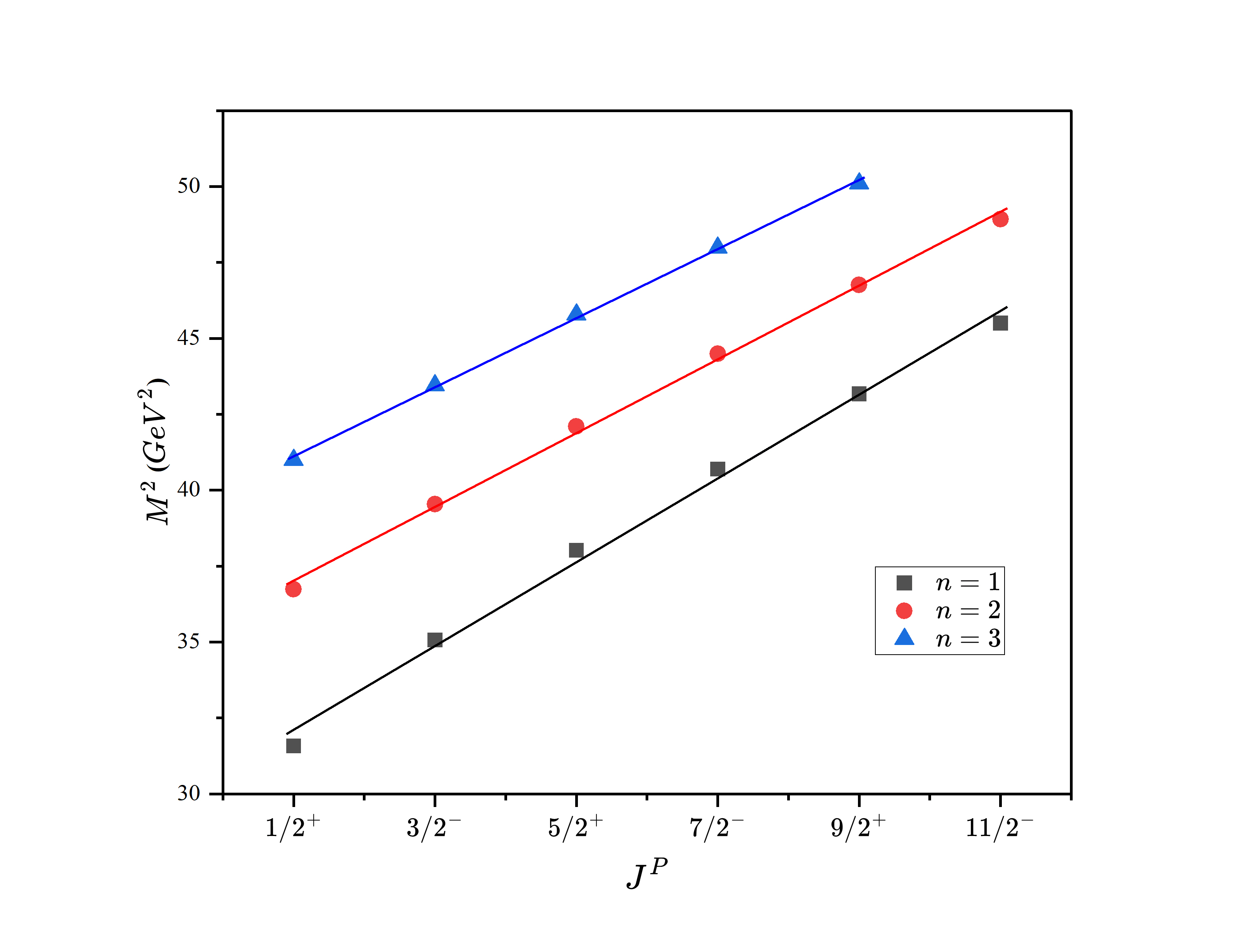
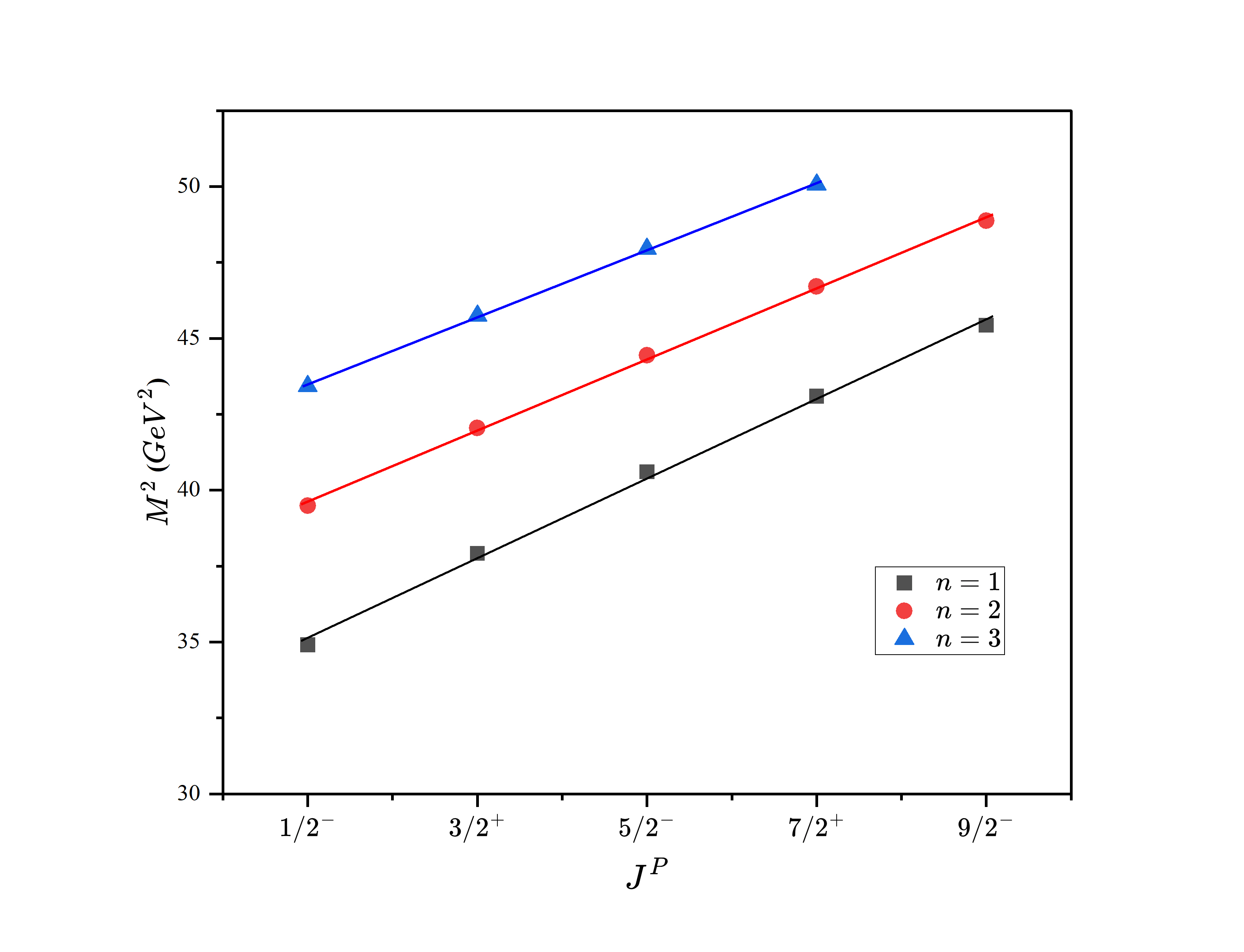
Figure 3: Regge trajectory in the ($J,M^{2}$) plane for $\Lambda_{b}$ baryonic family with natural parity states (left) and unnatural parity states (right).

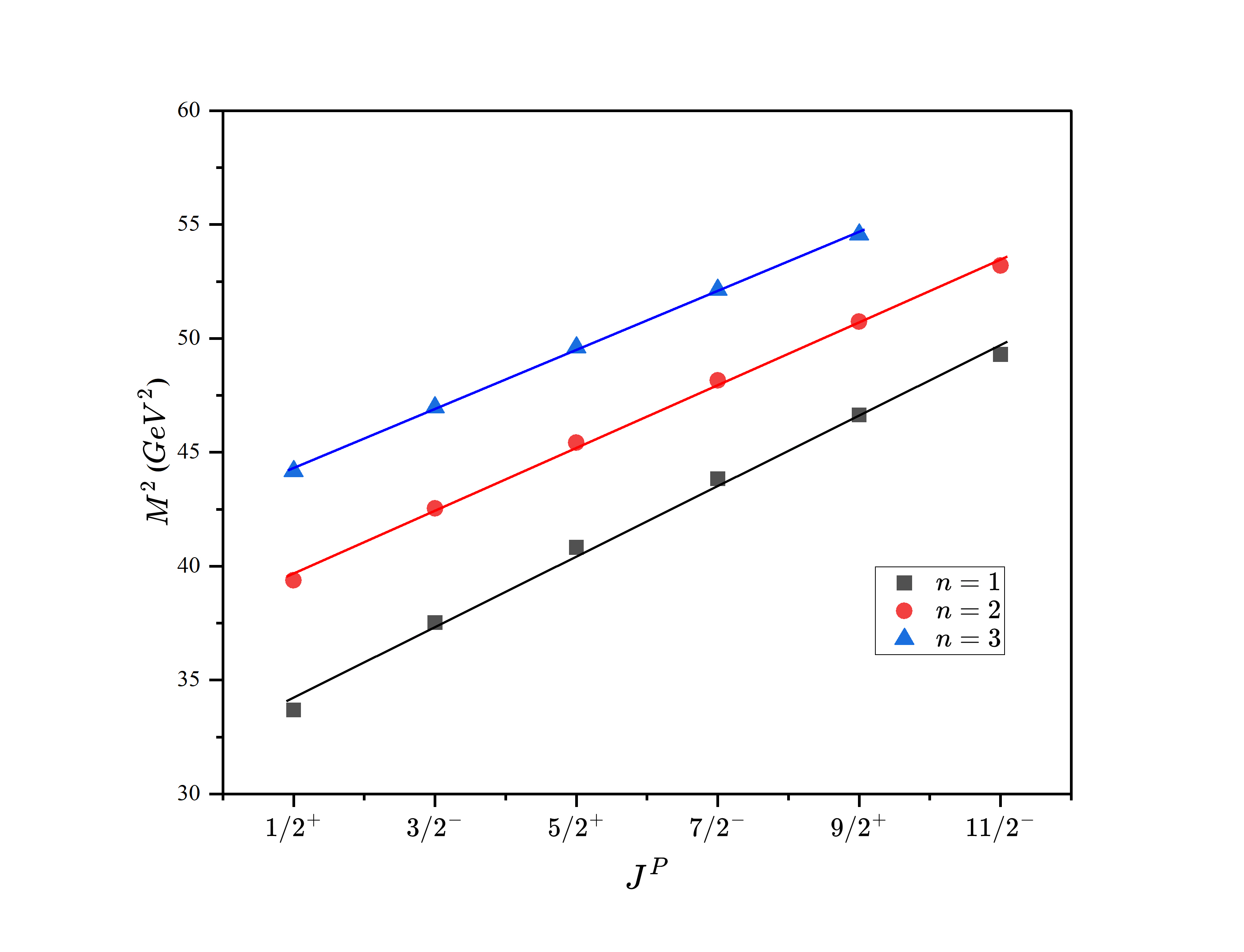
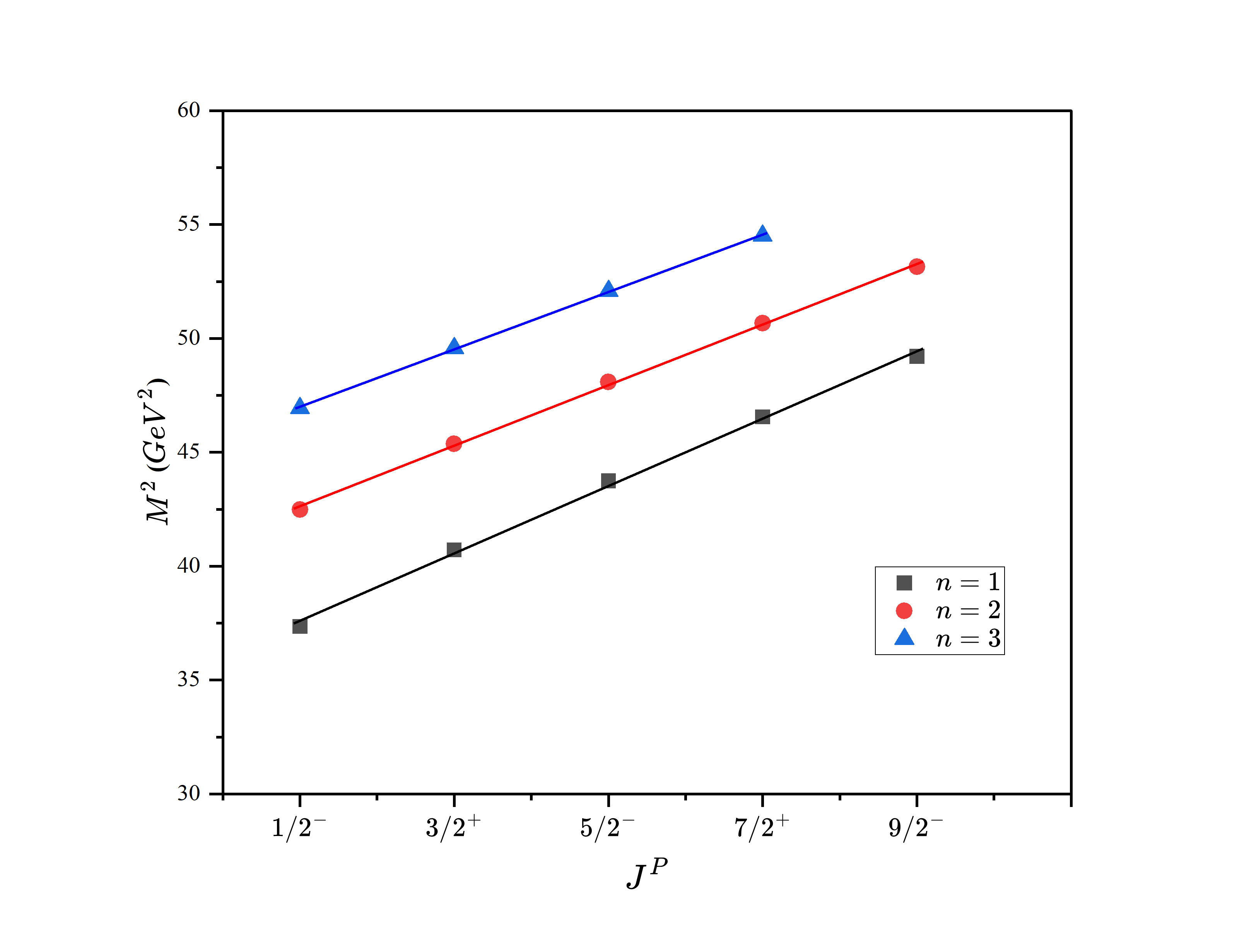
Figure 4: Regge trajectory in the ($J,M^{2}$) plane for $\Xi_{b}$ baryonic family with natural parity states (left) and unnatural parity states (right).

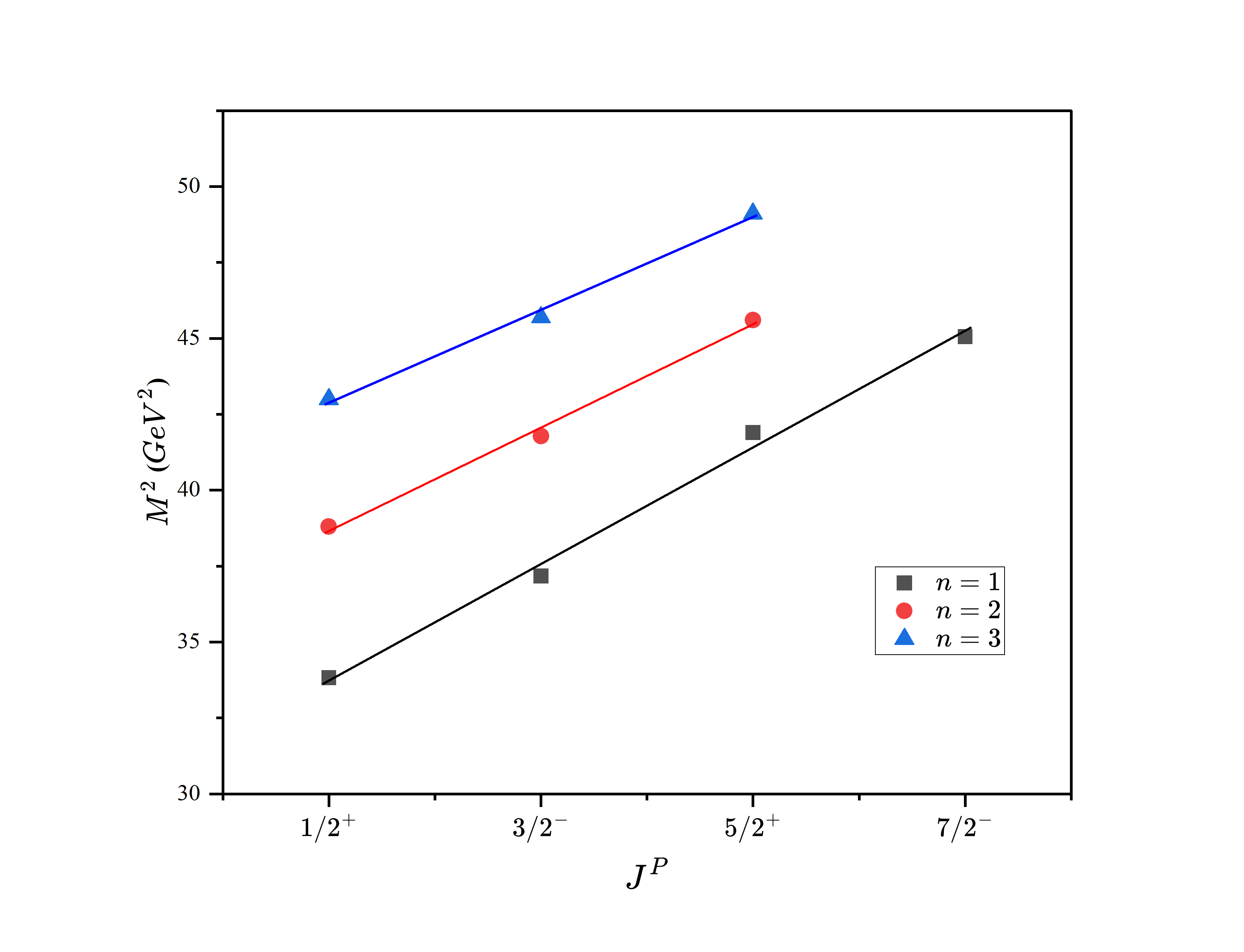
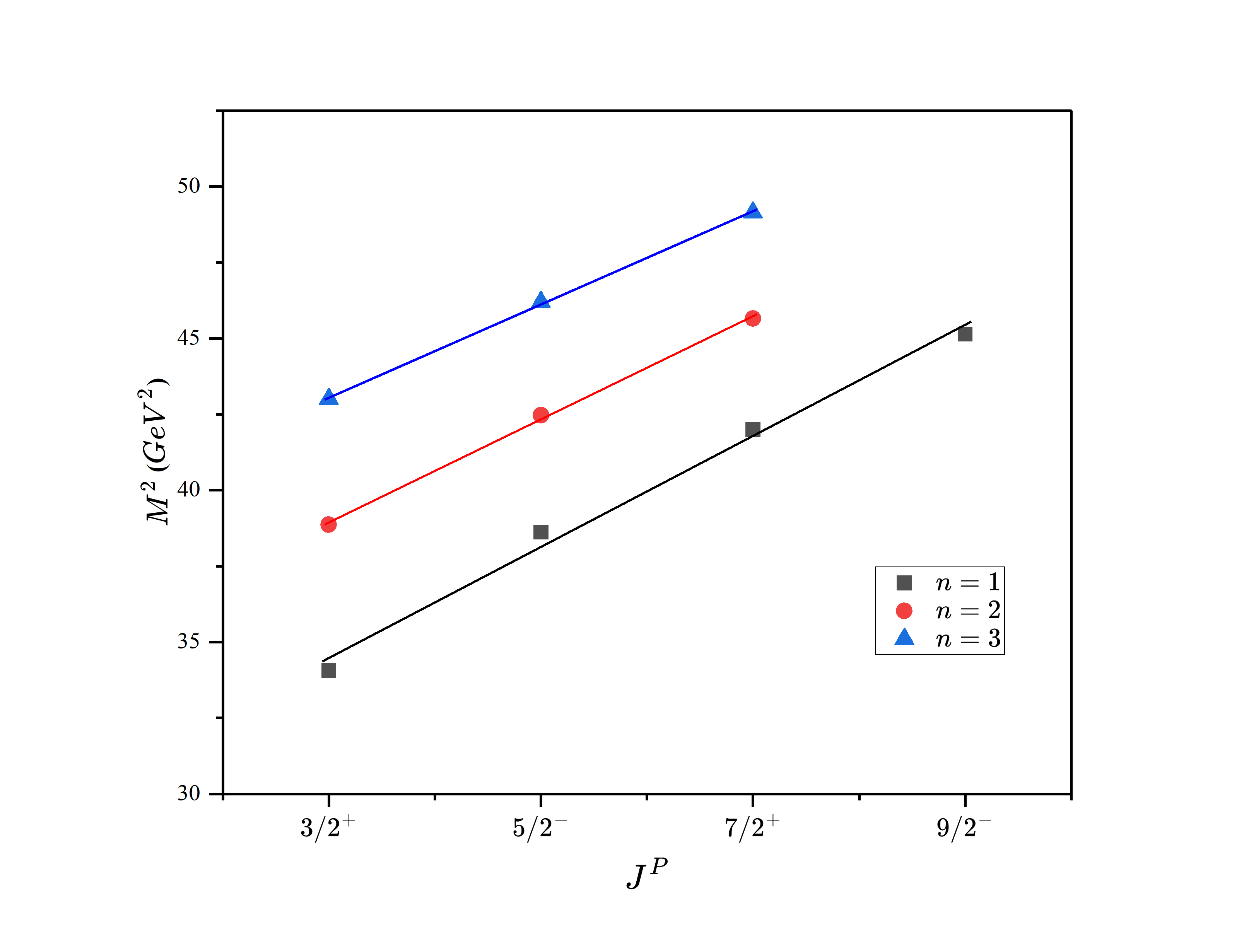
Figure 5: Regge trajectory in the ($J,M^{2}$) plane for $\Sigma_{b}$ baryonic family with natural parity states (left) and unnatural parity states (right).

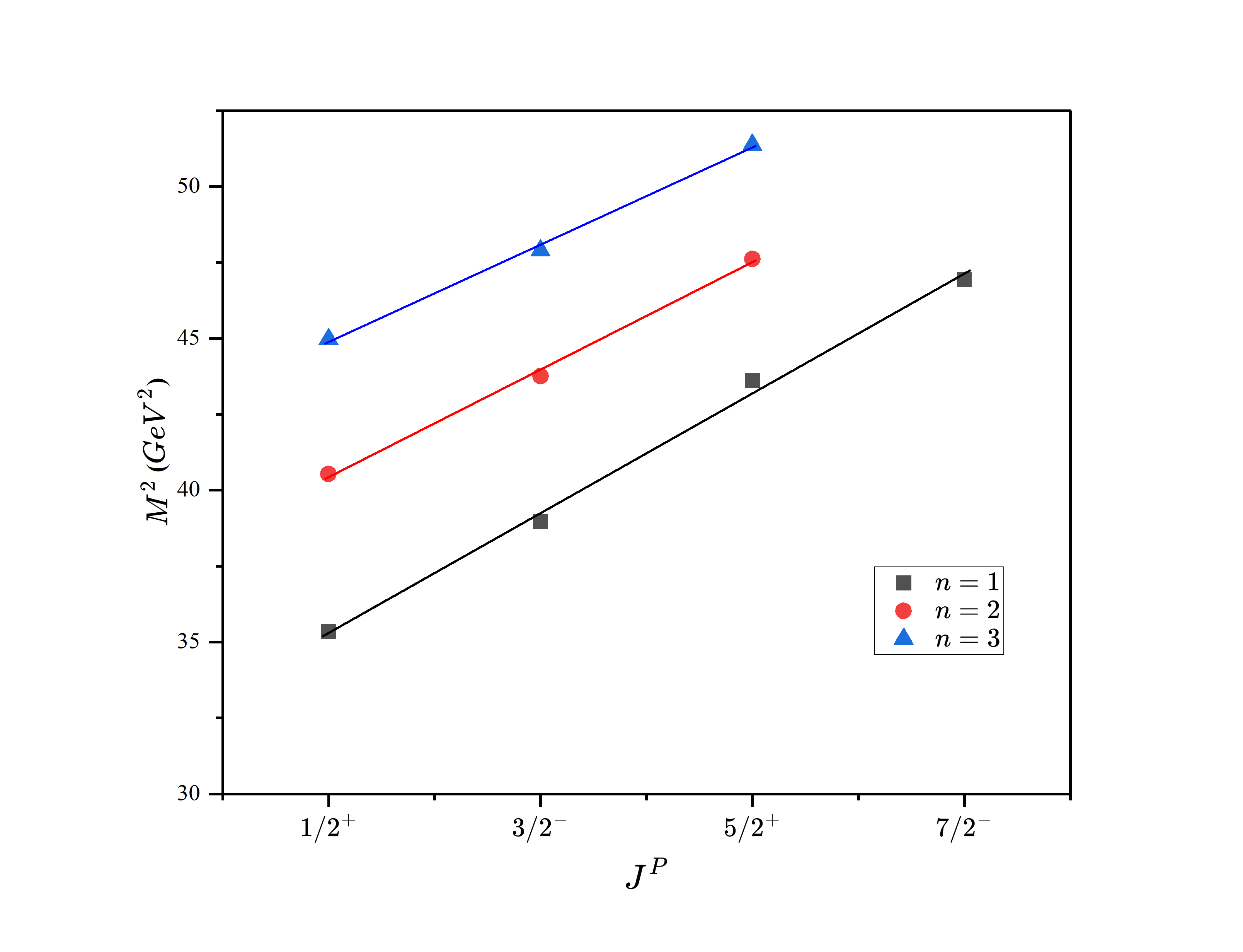
Figure 6: Regge trajectory in the ($J,M^{2}$) plane for $\Xi_{b}^{{}^{\prime}}$ baryonic family with natural parity states (left) and unnatural parity states (right).

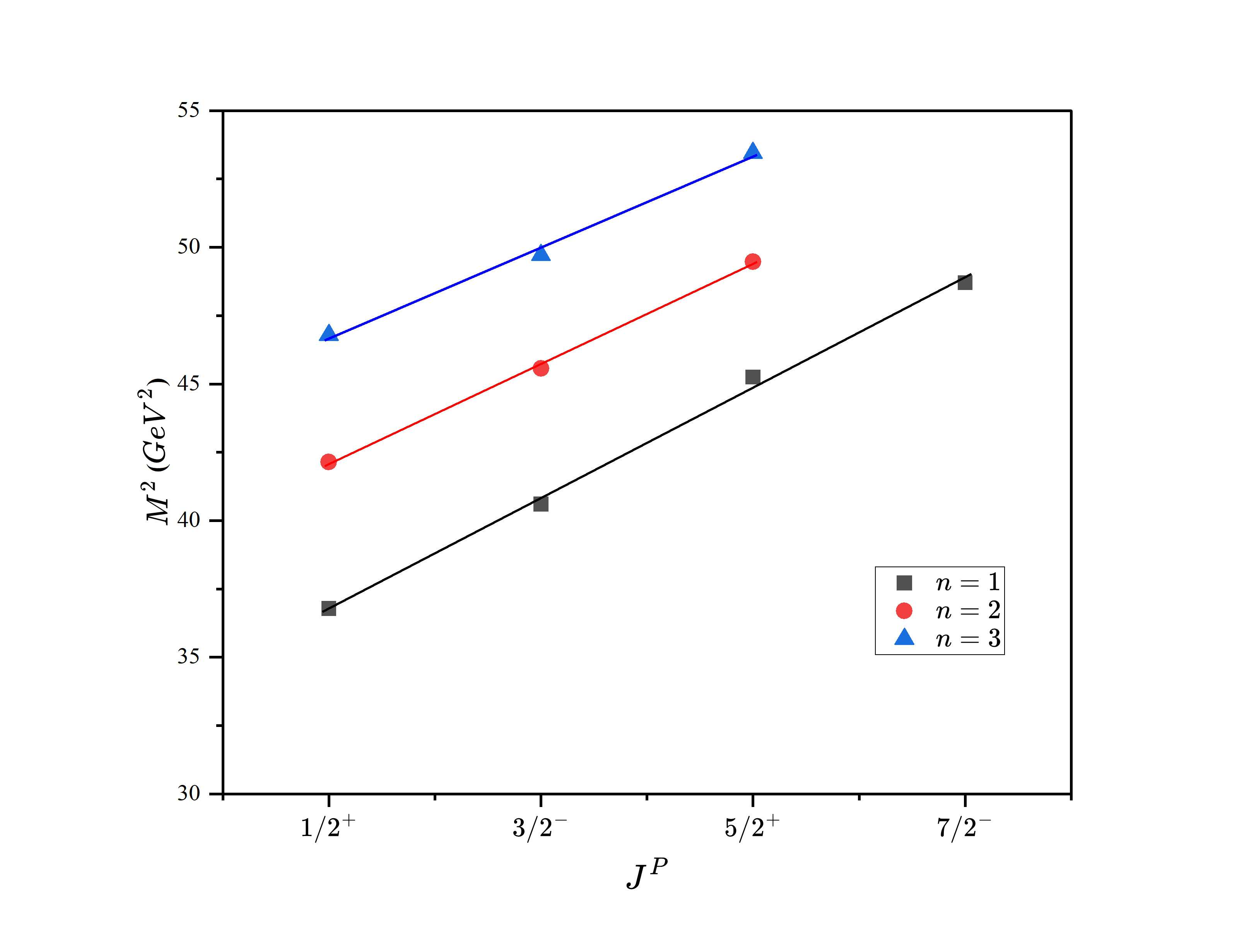
Figure 7: Regge trajectory in the ($J,M^{2}$) plane for $\Omega_{b}$ baryonic family with natural parity states (left) and unnatural parity states (right).

IV.2 $\Xi_{b}$ and $\Xi_{b}^{{}^{\prime}}$ baryons

For the $\Xi_{b}$ baryonic family, only the state belonging to ground state $|1S,1/2^{+}\rangle$ is established. Our calculated mass for this ground state is in good agreement with it, with a difference of only 6.6 MeV. The strong decay is forbidden for the ground state of $\Xi_{b}$ baryon. Recently, in 2021, the CMS experiment reported the $\Xi_{b}(6100)$ state in the $\Xi_{b}^{-}\pi^{+}\pi^{-}$ channel [17]. Its spin parity quantum numbers are not measured in this experiment. But based on similarities with known excited $\Xi_{c}$ baryon states, they predicted this state to be the orbitally excited $\Xi_{b}$ baryon, with spin-parity $J^{P}=\frac{3}{2}^{-}$. However, this spin parity has not yet been verified. Our calculated mass for the $|1P,1/2^{-}\rangle$ state falls very close to the experimentally measured mass of the $\Xi_{b}(6100)$ state, with a difference of only 11.5 MeV. Furthermore, as indicated in Table 7, the decay width of the $\Xi_{b}(6100)$ state closely aligns with the calculated strong decay width of the $|1P,1/2^{-}\rangle$ state compared to the calculated decay width of the $|1P,3/2^{-}\rangle$ state. Hence, we predict $\Xi_{b}(6100)$ state to be a good candidate of $1P$-wave with spin-parity $J^{P}=\frac{1}{2}^{-}$. The mass prediction in Ref.[19] is in favour of this assignment.

For the $\Xi_{b}^{{}^{\prime}}$ baryonic family, the states belonging to the $1S$-wave, with $J^{P}=\frac{1}{2}^{+}$ and $J^{P}=\frac{3}{2}^{+}$, are well determined. Our calculated masses for these states are very close to the experimental masses, with a difference of only 10 MeV and 7.3 MeV, respectively. The strong decay of the ground state of $\Xi_{b}^{{}^{\prime}}$ baryon is forbidden. But, our calculated strong decay width for $\Xi_{b}^{{}^{\prime}-}|1S,3/2^{+}\rangle$ and $\Xi_{b}^{{}^{\prime}0}|1S,3/2^{+}\rangle$ states is compatible with the decay width of the observed states $\Xi_{b}(5955)^{-}$ and $\Xi_{b}(5945)^{0}$, respectively. Further, the $\Xi_{b}(6227)^{-}$ state was observed by the LHCb experiment in the $\Xi_{b}^{0}\pi^{-}$ channel [10]. Later, the LHCb experiment in the $\Xi_{b}^{-}\pi^{+}$ channel observed its isospin partner named $\Xi_{b}(6227)^{0}$. The spin-parity quantum numbers of this state are not yet identified. Our calculated masses for $|1P,1/2^{-}\rangle_{j=1}$ and $|1P,3/2^{-}\rangle_{j=1}$ states of $\Xi_{b}^{{}^{\prime}}$ baryon   are  close to the experimental mass of the $\Xi_{b}(6227)$ baryon. However, the decay width of the $\Xi_{b}(6227)$ state is nearly identical to the strong decay width of the $|1P,3/2^{-}\rangle_{j=1}$ state, which eliminates the possibility of it being the $|1P,1/2^{-}\rangle_{j=1}$ state. Therefore, we identify the $\Xi_{b}(6227)$ baryon as the first orbital excitation ($1P$) of $\Xi_{b}^{{}^{\prime}}$ baryon with  $J^{P}=\frac{3}{2}^{-}$. This assignment is confirmed by Ref.[55]. While in Ref. [19, 22] the predicted masses of states in the $1P$-wave of $\Xi_{b}^{{}^{\prime}}$ baryon are too close to assign specific spin-parity to $\Xi_{b}(6227)$. However, these predictions do provide support for our argument that the $\Xi_{b}(6227)$ belongs to the $1P$-wave of the $\Xi_{b}^{{}^{\prime}}$ baryon. The authors in Ref.[20] also support this argument, but they predict it’s spin-parity to be $J^{P}=\frac{5}{2}^{-}$. At last, in 2021, the LHCb collaboration has observed $\Xi_{b}(6327)$ and $\Xi_{b}(6333)$ states in the $\Lambda_{b}^{0}K^{-}\pi^{+}$ channel [18]. The spin-parity of it is still a mystery. The masses and decay widths of these states were in agreement with the predictions made in Ref.[62, 63] for $1D$-wave $\Xi_{b}$ baryonic states with $J^{P}=\frac{3}{2}^{-}$ and $\frac{5}{2}^{-}$. However, we observe that the masses of $\Xi_{b}(6327)$ and $\Xi_{b}(6333)$ are very close to our predicted masses for the $|1P,3/2^{-}\rangle_{j=2}$ and $|1P,5/2^{-}\rangle$ states of the $\Xi_{b}^{{}^{\prime}}$ baryonic family. Hence, we suggest the alternative possibility that $\Xi_{b}(6327)$ and $\Xi_{b}(6333)$ can be components of the first orbital excitation ($1P$) of the $\Xi_{b}^{{}^{\prime}}$ baryonic family, with $J^{P}=\frac{3}{2}^{-}$ and $\frac{5}{2}^{-}$, respectively.

IV.3 $\Sigma_{b}$ baryons

The $\Sigma_{b}$ baryonic family has very well established states in the $1S$ wave. Our calculated mass for the $1S$ wave with quantum numbers $J^{P}=\frac{1}{2}^{+}$ and $J^{P}=\frac{3}{2}^{+}$ is very close to the experimental masses of these states, with a difference of 5.64 MeV and 6.68 MeV only. As indicated in Table 7, their widths are also well reproduced in our model.

Further, the LHCb Collaboration has been able to detect only one excited state of the $\Sigma_{b}$ baryon so far, named $\Sigma_{b}(6097)$ in the $\Lambda_{c}^{+}K^{-}\pi^{+}\pi^{-}$ mass spectrum [11]. The quantum numbers of this state are not confirmed yet. The experimental mass of this state is in excellent match with our predicted mass for the $|1P,3/2^{-}\rangle_{j=1}$ state. In addition, the decay width of $\Sigma_{b}(6097)$ also closely matches the strong decay width of $|1P,3/2^{-}\rangle_{j=1}$ state. This clearly indicates that $\Sigma_{b}(6097)$ is a potential candidate for a $1P$- wave with a spin-parity  $J^{P}=\frac{3}{2}^{-}$. This assignment is also supported by ref. [55, 64, 65].

IV.4 $\Omega_{b}$ baryons

For $\Omega_{b}$ baryons, only the ground state is established. Our calculated mass for the ground state deviates slightly by 20 MeV from its experimental mass. Further, the LHCb collaboration [66] has reported four narrow states in the $\Xi_{b}^{0}K^{-}$ spectrum, designated as $\Omega_{b}(6316)$, $\Omega_{b}(6330)$, $\Omega_{b}(6340)$, and $\Omega_{b}(6350)$. These states have masses ranging from 6315 to 6350 MeV, though their spin parity remains unmeasured. Similarly, the LHCb collaboration [67] has observed five narrow states of the $\Omega_{c}$ baryonic family, named $\Omega_{c}(3000)$,  $\Omega_{c}(3050)$,  $\Omega_{c}(3065)$,  $\Omega_{c}(3090)$, and $\Omega_{c}(3120)$. In our previous work [43], we have interpreted them as the $1P$-wave excitations of $\{s,s\}$ diquark with respect to the charm quark. The discovery of these narrow states in both the $\Omega_{b}$ and $\Omega_{c}$ families reinforces the notion of similar excitation mechanisms in doubly strange baryons containing one heavy quark.

As shown in Table 6, the masses of four experimentally observed excited states of $\Omega_{b}$ baryon lie comparatively close to the masses of the $1P$-wave states, named $|1P,1/2^{-}\rangle_{j=0}$, $|1P,1/2^{-}\rangle_{j=1}$, $|1P,3/2^{-}\rangle_{j=1}$, and $|1P,3/2^{-}\rangle_{j=2}$. Therefore, it is possible that these four narrow states belong to the $1P$-wave. However, in our calculated mass spectra, the mass splitting in the $1P$-wave is large, resulting in a considerable difference between the calculated masses of the $1P$-wave states and the masses of experimentally detected states. A potential reason for large splitting in $1P$-wave could be our underlying assumption that the $\Omega_{b}$ baryon follows the heavy quark symmetry. This assumption has led us to calculate the spin-dependent splitting in the j-j coupling scheme. However, it may not be the most effective coupling scheme for the $\Omega_{b}$ baryon, which consists of two strange quarks. This suggests that an alternative coupling scheme must be developed in order to study the mass spectra of $\Omega_{b}$ baryons in the relativistic flux tube model.

Based on calculation of strong decay widths, we cannot definitively determine the spin-parity assignments for the observed excited states of the $\Omega_{b}$ baryon. The calculated widths for $|1P,1/2^{-}\rangle_{j=0}$ is too broad to be observed, while the range of widths for $|1P,3/2^{-}\rangle_{j=1}$ and $|1P,3/2^{-}\rangle_{j=2}$ are too large to firmly associate any experimental state with them. Additionally, for the remaining two states in the $1P$-wave, strong decay channels are suppressed by phase space constraint in our model. Hence, further theoretical and experimental research is required to identify these four resonances of $\Omega_{b}$ baryon.

V CONCLUSION AND OUTLOOK

We have conducted computations for the mass spectra of single-bottom baryons. In the relativistic flux tube model, single-bottom baryons are pictured as a two-body system consisting of a bottom quark and a diquark. The additional spin-dependent interactions are also taken into account in the j-j coupling scheme. It is essential to mention that our approach does not include parameter fitting. Instead, the parameters of our model were determined earlier by using the masses of experimentally reported states of singly charmed baryons and some low lying states of $\Lambda_{b}$ baryon as inputs. Therefore, it provide a unified description of both singly charmed and bottom baryons. In various quark model calculations [19, 20], model parameters are typically adjusted to fit the ground state or a lower excited state, resulting in a close match to experimentally measured masses for the ground state. However, In that approach the discrepancies between model predictions and experimental data become more pronounced for higher excited states such as $1D$-wave states of $\Lambda_{b}$ baryon and $1P$-wave states of $\Xi_{b}$ baryon. While in our approach, we found that the calculated masses for excited states of $\Lambda_{b}$, $\Xi_{b}$, $\Sigma_{b}$,and $\Xi_{b}^{{}^{\prime}}$ baryons are closer to the experimentally measured masses. Therefore, our model prediction for the excited state masses are more reliable. The Regge trajectories obtained from the calculated masses are observed to be almost linear, parallel, and equidistant in the $(J,M^{2})$ plane. The masses and strong decay width of experimentally observed states of $\Lambda_{b}$, $\Xi_{b}$, $\Sigma_{b}$, and $\Xi_{b}^{\prime}$ are well reproduced in this theoretical framework. Based on this, we have assigned possible spin-parity quantum numbers to $\Sigma_{b}(6097)$, $\Xi_{b}(6100)$, $\Xi_{b}(6227)$, $\Xi_{b}(6327)$, and $\Xi_{b}(6333)$, which might be useful to establish them in their mass spectra. Ongoing experimental research on single-bottom baryons at LHCb is expected to discover new states with increasing luminosity and energy in the future. Our theoretical predictions for the masses of higher-lying states can assist experimentalists in identifying and investigating certain resonances in the spectrum of singly bottom baryons.

For the $\Omega_{b}$ baryonic family, as the experimentally measured masses of $\Omega_{b}(6316)$, $\Omega_{b}(6330)$, $\Omega_{b}(6340)$, and $\Omega_{b}(6350)$ fall close to the theoretical masses of $1P$-wave states in the quark-diquark picture. But, with the j-j coupling scheme in our model, we observe significant spin-dependent mass splitting in the $1P$-wave. To accurately reproduce the experimental masses of $\Omega_{b}$ baryons, a different coupling scheme needs to be introduced. In the future, it would be interesting to explore an alternative coupling scheme for studying the mass spectra of $\Omega_{b}$ baryons in the relativistic flux tube model.

Appendix

We have already demonstrated how to compute the expectation values of operators involved in spin dependent interactions for $S$-wave, $P$-wave, and $D$-wave of singly heavy baryons having vector diquarks in our earlier work [43]. In this section, we will extend our calculation to the case of $F$-wave and $G$-wave of singly heavy baryons having vector diquark.

1. The F-wave:

   The $L-S$ coupling scheme involves coupling of $\mathbf{S_{\mathcal{D}}}$ and $\mathbf{S_{b}}$ to form $\mathbf{S}$, and then coupling $\mathbf{S}$ and $\mathbf{L}$ to get the total angular momentum $\mathbf{J}$. Using uncoupled states $|S_{\mathcal{D}},S_{\mathcal{D}_{3}}\rangle$, $|S_{b},S_{b_{3}}\rangle$, and $|L,L_{3}\rangle$ , we can construct the $L-S$ coupling basis states as [43]

   $$|(S_{\mathcal{D}}S_{b})SL;J\ J_{3}\rangle=\displaystyle\sum_{\scriptscriptstyle{S_{\mathcal{D}_{3}}S_{b_{3}}L_{3}}S_{3}}C_{S_{\mathcal{D}_{3}}S_{b_{3}}S_{3}}^{S_{\mathcal{D}}\ S_{b}\ S}\ C_{S_{3}L_{3}J_{3}}^{S\ L\ J}\ |S_{\mathcal{D}}S_{\mathcal{D}_{3}}\rangle|S_{b}S_{b_{3}}\rangle|L\ L_{3}\rangle,$$ (29)

   where, $S_{\mathcal{D}_{3}}$, $S_{b_{3}}$, $L_{3}$ and $J_{3}$ signify the third component of $\mathbf{S_{\mathcal{D}}}$, $\mathbf{S_{b}}$, $\mathbf{L}$ and $\mathbf{J}$, respectively. ${C_{S_{\mathcal{D}_{3}}S_{b_{3}}S_{3}}^{S_{\mathcal{D}}\ S_{b}\ S}}$ and $C_{S_{3}L_{3}J_{3}}^{S\ L\ J}$ are Clebsch-Gordan coefficients. For the sake of convenience, We use $|^{2S+1}L_{J};J_{3}\rangle$ to denote the basis $|(S_{\mathcal{D}}S_{b})SL;J\ J_{3}\rangle$ and $|S_{\mathcal{D}_{3}},S_{b_{3}},L_{3}\rangle$ to denote the product of states $|S_{\mathcal{D}}S_{\mathcal{D}_{3}}\rangle|S_{b}S_{b_{3}}\rangle|L\ L_{3}\rangle$ for fixed values of $S_{\mathcal{D}}$, $S_{b}$ and $L$. Following that, Eq. [29] is rewritten as

   $$|^{2S+1}L_{J};J_{3}\rangle=\displaystyle\sum_{\scriptscriptstyle{S_{\mathcal{D}_{3}}S_{b_{3}}L_{3}}S_{3}}C_{S_{\mathcal{D}_{3}}S_{b_{3}}S_{3}}^{S_{\mathcal{D}}\ S_{b}\ S}\ C_{S_{3}L_{3}J_{3}}^{S\ L\ J}\ |S_{\mathcal{D}_{3}},S_{b_{3}},L_{3}\rangle.$$ (30)

   Based on the relation above, we can list the $L-S$ coupling basis states for $F$-wave as follows:

   $$|^{4}F_{3/2};3/2\rangle=-\frac{2}{\sqrt{7}}|-1,-\frac{1}{2},3\rangle+\frac{2}{\sqrt{21}}|0,-\frac{1}{2},2\rangle-\frac{2}{\sqrt{105}}|1,-\frac{1}{2},1\rangle+\sqrt{\frac{2}{21}}|-1,\frac{1}{2},2\rangle-2\sqrt{\frac{2}{105}}|0,\frac{1}{2},1\rangle+\frac{1}{\sqrt{35}}|1,\frac{1}{2},0\rangle,$$ (31)

   $$|^{2}F_{5/2};5/2\rangle=-\sqrt{\frac{2}{7}}|0,-\frac{1}{2},3\rangle+\sqrt{\frac{2}{21}}|1,-\frac{1}{2},2\rangle+\frac{2}{\sqrt{7}}|-1,\frac{1}{2},3\rangle-\frac{1}{\sqrt{21}}|0,\frac{1}{2},2\rangle,$$ (32)

   $$|^{4}F_{5/2};5/2\rangle=\sqrt{\frac{5}{14}}|0,-\frac{1}{2},3\rangle-\sqrt{\frac{5}{42}}|1,-\frac{1}{2},2\rangle+\frac{1}{2}\sqrt{\frac{5}{7}}|-1,\frac{1}{2},3\rangle-\sqrt{\frac{5}{21}}|0,\frac{1}{2},2\rangle+\frac{1}{2}\sqrt{\frac{3}{7}}|1,\frac{1}{2},1\rangle,$$ (33)

   $$|^{2}F_{7/2};7/2\rangle=\sqrt{\frac{2}{3}}|1,-\frac{1}{2},3\rangle-\frac{1}{\sqrt{3}}|0,\frac{1}{2},3\rangle,$$ (34)

   $$|^{4}F_{7/2};7/2\rangle=-\frac{\sqrt{2}}{3}|1,-\frac{1}{2},3\rangle-\frac{2}{3}|0,\frac{1}{2},3\rangle+\frac{1}{\sqrt{3}}|1,\frac{1}{2},2\rangle,$$ (35)

   $$|^{4}F_{9/2};9/2\rangle=|1,\frac{1}{2},3\rangle,$$ (36)

   We can simplify the operators that are involved in spin-dependent interactions as below:

   $$\mathbf{L\cdot S_{i}}=\frac{1}{2}\left[L_{+}S_{i-}+L_{-}S_{i+}\right]+L_{3}S_{i3},$$ (37)

   where $i=\mathcal{D}$ or $b$, and
   

   $$\mathbf{\hat{B}}=\frac{-3}{(2L-1)(2L+3)}\left[(\mathbf{L\cdot S_{\mathcal{D}}})(\mathbf{L\cdot S_{b}})+(\mathbf{L\cdot S_{b}})(\mathbf{L\cdot S_{\mathcal{D}}})-\frac{2}{3}L(L+1)(\mathbf{S_{\mathcal{D}}\cdot S_{b}})\right].$$ (38)

   The expression for the expectation value of $\mathbf{S_{\mathcal{D}}}\cdot\mathbf{S_{b}}$ in $L-S$ coupling basis is

   $$\langle\mathbf{S_{\mathcal{D}}}\cdot\mathbf{S_{b}}\rangle=\frac{1}{2}[S(S+1)-S_{\mathcal{D}}(S_{\mathcal{D}}+1)-S_{b}(S_{b}+1)].$$ (39)

   Then, we find the expectation values of spin-dependent operators in $[^{2}F_{J},^{4}F_{J}]$ basis for different J values, and the outcomes are given below:

   For J=3/2,

   $$\text{{\hbox{\langle\mathbf{L}\cdot\mathbf{S_\mathcal{D}}\rangle}} =}-4,\ \text{{\hbox{\langle\mathbf{L}\cdot\mathbf{S_b}\rangle}} =}-2,\ \text{{\hbox{\langle\mathbf{\hat{B}} \rangle}}=}-\frac{4}{5},\ \text{{\hbox{\langle\mathbf{S_\mathcal{D}}\cdot\mathbf{S_b}\rangle}}=}\frac{1}{2}.$$ (40)

   For J=5/2,

   $$\text{{\hbox{\langle\mathbf{L}\cdot\mathbf{S_\mathcal{D}}\rangle}}=}\left[\begin{array}[]{cc}-\frac{8}{3}&-\frac{2\sqrt{5}}{3}\\[5.0pt] -\frac{2\sqrt{5}}{3}&-\frac{7}{3}\\[1.0pt] \end{array}\right],\ \ \text{{\hbox{\langle\mathbf{L}\cdot\mathbf{S_b}\rangle}}=}\left[\begin{array}[]{cc}\frac{2}{3}&\frac{2\sqrt{5}}{3}\\[5.0pt] \frac{2\sqrt{5}}{3}&-\frac{7}{6}\\[1.0pt] \end{array}\right],\ \ \text{{\hbox{\langle\mathbf{\hat{B}} \rangle}}=}\left[\begin{array}[]{cc}0&\frac{1}{\sqrt{5}}\\[5.0pt] \frac{1}{\sqrt{5}}&\frac{1}{5}\\[1.0pt] \end{array}\right],\ \ \text{{\hbox{\langle\mathbf{S_\mathcal{D}}\cdot\mathbf{S_b}\rangle}}=}\left[\begin{array}[]{cc}-1&0\\[5.0pt] 0&\frac{1}{2}\\[1.0pt] \end{array}\right].$$ (41)

   For J=7/2,

   $$\text{{\hbox{\langle\mathbf{L}\cdot\mathbf{S_\mathcal{D}}\rangle}}=}\left[\begin{array}[]{cc}2&-\sqrt{3}\\[5.0pt] -\sqrt{3}&0\\[1.0pt] \end{array}\right],\ \ \text{{\hbox{\langle\mathbf{L}\cdot\mathbf{S_b}\rangle}}=}\left[\begin{array}[]{cc}-\frac{1}{2}&\sqrt{3}\\[5.0pt] \sqrt{3}&0\\[1.0pt] \end{array}\right],\ \ \text{{\hbox{\langle\mathbf{\hat{B}} \rangle}}=}\left[\begin{array}[]{cc}0&-\frac{1}{2\sqrt{3}}\\[5.0pt] -\frac{1}{2\sqrt{3}}&\frac{2}{3}\\[1.0pt] \end{array}\right],\ \ \text{{\hbox{\langle\mathbf{S_\mathcal{D}}\cdot\mathbf{S_b}\rangle}}=}\left[\begin{array}[]{cc}-1&0\\[5.0pt] 0&\frac{1}{2}\\[1.0pt] \end{array}\right].$$ (42)

   For J=9/2,

   $$\text{{\hbox{\langle\mathbf{L}\cdot\mathbf{S_\mathcal{D}}\rangle}} =}3,\ \text{{\hbox{\langle\mathbf{L}\cdot\mathbf{S_b}\rangle}} =}\frac{3}{2},\ \text{{\hbox{\langle\mathbf{\hat{B}} \rangle}}=}-\frac{1}{3},\ \text{{\hbox{\langle\mathbf{S_\mathcal{D}}\cdot\mathbf{S_b}\rangle}}=}\frac{1}{2}.$$ (43)

   Here, we observe that the dominant interaction term in spin-dependent interaction, i.e., $\langle\mathbf{L}\cdot\mathbf{S_{\mathcal{D}}}\rangle$, is not diagonal for $J=5/2$ and $J=7/2$, in   $[^{2}F_{J},^{4}F_{J}]$ basis of the $L-S$ coupling scheme.

   But in the $j-j$ coupling scheme, they are diagonal. To find expectation values of these operators in the $j-j$ coupling scheme, we start with finding eigen functions corresponding to each eigen value $k$ of $\langle\mathbf{L}\cdot\mathbf{S_{\mathcal{D}}}\rangle$ which forms the basis in $j-j$ coupling scheme, as shown below:

   $$|J=\frac{3}{2},j=2\rangle=|^{4}F_{3/2}\rangle$$ (44)

   $$k=-4:|J=\frac{5}{2},j=2\rangle=\frac{\sqrt{5}}{3}|^{2}F_{5/2}\rangle+\frac{2}{3}|^{4}F_{5/2}\rangle,$$ (45)

   $$k=-1:|J=\frac{5}{2},j=3\rangle=-\frac{2}{3}|^{2}F_{5/2}\rangle+\frac{\sqrt{5}}{3}|^{4}F_{5/2}\rangle,$$ (46)

   $$k=3:|J=\frac{7}{2},j=3\rangle=-\frac{\sqrt{3}}{2}|^{2}F_{7/2}\rangle+\frac{1}{2}|^{4}F_{7/2}\rangle,$$ (47)

   $$k=-1:|J=\frac{7}{2},j=4\rangle=\frac{1}{2}|^{2}F_{7/2}\rangle+\frac{\sqrt{3}}{2}|^{4}F_{7/2}\rangle,$$ (48)

   $$|J=\frac{9}{2},j=4\rangle=|^{4}F_{9/2}\rangle$$ (49)

   Following that, we compute the expectation value of spin-dependent operators in a $|J,j\rangle$ basis and display the results in a Table 1.

2. The G-wave: We start with forming the $L-S$ coupling states as a linear combination of uncoupled states $|S_{\mathcal{D}_{3}},S_{b_{3}},L_{3}\rangle$, using Eq.(30), as follows:

   $$|^{4}G_{5/2};5/2\rangle=-\sqrt{\frac{2}{3}}|-1,-\frac{1}{2},4\rangle+\frac{1}{\sqrt{6}}|0,-\frac{1}{2},3\rangle-\frac{1}{\sqrt{42}}|1,-\frac{1}{2},2\rangle+\frac{1}{2\sqrt{3}}|-1,\frac{1}{2},3\rangle-\frac{1}{\sqrt{21}}|0,\frac{1}{2},2\rangle+\frac{1}{2\sqrt{21}}|1,\frac{1}{2},1\rangle,$$ (50)

   $$|^{2}G_{7/2};7/2\rangle=-\frac{2}{3}\sqrt{\frac{2}{3}}|0,-\frac{1}{2},4\rangle+\frac{1}{3}\sqrt{\frac{2}{3}}|1,-\frac{1}{2},3\rangle+\frac{4}{3\sqrt{3}}|-1,\frac{1}{2},4\rangle-\frac{1}{3\sqrt{3}}|0,\frac{1}{2},3\rangle,$$ (51)

   $$|^{4}G_{7/2};7/2\rangle=\frac{2}{3}\sqrt{\frac{14}{15}}|0,-\frac{1}{2},4\rangle-\frac{1}{3}\sqrt{\frac{14}{15}}|1,-\frac{1}{2},3\rangle+\frac{2}{3}\sqrt{\frac{7}{15}}|-1,\frac{1}{2},4\rangle-\frac{2}{3}\sqrt{\frac{7}{15}}|0,\frac{1}{2},3\rangle+\frac{1}{\sqrt{15}}|1,\frac{1}{2},2\rangle,$$ (52)

   $$|^{2}G_{9/2};9/2\rangle=\sqrt{\frac{2}{3}}|1,-\frac{1}{2},4\rangle-\frac{1}{\sqrt{3}}|0,\frac{1}{2},4\rangle,$$ (53)

   $$|^{4}G_{9/2};9/2\rangle=-2\sqrt{\frac{2}{33}}|1,-\frac{1}{2},4\rangle-\frac{4}{\sqrt{33}}|0,\frac{1}{2},4\rangle+\sqrt{\frac{3}{11}}|1,\frac{1}{2},3\rangle,$$ (54)

   $$|^{4}G_{11/2};11/2\rangle=|1,\frac{1}{2},4\rangle,$$ (55)

   Following that, the expectation values of spin-dependent operators in $[^{2}G_{J},^{4}G_{J}]$ basis are calculated for different values of $J$ and the results are listed below: For J=5/2,

   $$\text{{\hbox{\langle\mathbf{L}\cdot\mathbf{S_\mathcal{D}}\rangle}} =}-5,\ \text{{\hbox{\langle\mathbf{L}\cdot\mathbf{S_b}\rangle}} =}-\frac{5}{2},\ \text{{\hbox{\langle\mathbf{\hat{B}} \rangle}}=}-\frac{5}{7},\ \text{{\hbox{\langle\mathbf{S_\mathcal{D}}\cdot\mathbf{S_b}\rangle}}=}\frac{1}{2}.$$ (56)

   For J=7/2,

   $$\text{{\hbox{\langle\mathbf{L}\cdot\mathbf{S_\mathcal{D}}\rangle}}=}\left[\begin{array}[]{cc}-\frac{10}{3}&-\frac{\sqrt{35}}{3}\\[5.0pt] -\frac{\sqrt{35}}{3}&-\frac{8}{3}\\[1.0pt] \end{array}\right],\ \ \text{{\hbox{\langle\mathbf{L}\cdot\mathbf{S_b}\rangle}}=}\left[\begin{array}[]{cc}\frac{5}{6}&\frac{\sqrt{35}}{3}\\[5.0pt] \frac{\sqrt{35}}{3}&-\frac{4}{3}\\[1.0pt] \end{array}\right],\ \ \text{{\hbox{\langle\mathbf{\hat{B}} \rangle}}=}\left[\begin{array}[]{cc}0&\frac{1}{2}\sqrt{\frac{5}{7}}\\[5.0pt] \frac{1}{2}\sqrt{\frac{5}{7}}&\frac{2}{7}\\[1.0pt] \end{array}\right],\ \ \text{{\hbox{\langle\mathbf{S_\mathcal{D}}\cdot\mathbf{S_b}\rangle}}=}\left[\begin{array}[]{cc}-1&0\\[5.0pt] 0&\frac{1}{2}\\[1.0pt] \end{array}\right].$$ (57)

   For J=9/2,

   $$\text{{\hbox{\langle\mathbf{L}\cdot\mathbf{S_\mathcal{D}}\rangle}}=}\left[\begin{array}[]{cc}\frac{8}{3}&-\frac{2\sqrt{11}}{3}\\[5.0pt] -\frac{2\sqrt{11}}{3}&\frac{1}{3}\\[1.0pt] \end{array}\right],\ \ \text{{\hbox{\langle\mathbf{L}\cdot\mathbf{S_b}\rangle}}=}\left[\begin{array}[]{cc}-\frac{2}{3}&\frac{2\sqrt{11}}{3}\\[5.0pt] \frac{2\sqrt{11}}{3}&\frac{1}{6}\\[1.0pt] \end{array}\right],\ \ \text{{\hbox{\langle\mathbf{\hat{B}} \rangle}}=}\left[\begin{array}[]{cc}0&-\frac{1}{\sqrt{11}}\\[5.0pt] -\frac{1}{\sqrt{11}}&\frac{7}{11}\\[1.0pt] \end{array}\right],\ \ \text{{\hbox{\langle\mathbf{S_\mathcal{D}}\cdot\mathbf{S_b}\rangle}}=}\left[\begin{array}[]{cc}-1&0\\[5.0pt] 0&\frac{1}{2}\\[1.0pt] \end{array}\right].$$ (58)

   For J=11/2,

   $$\text{{\hbox{\langle\mathbf{L}\cdot\mathbf{S_\mathcal{D}}\rangle}} =}4,\ \text{{\hbox{\langle\mathbf{L}\cdot\mathbf{S_b}\rangle}} =}2,\ \text{{\hbox{\langle\mathbf{\hat{B}} \rangle}}=}-\frac{4}{11},\ \text{{\hbox{\langle\mathbf{S_\mathcal{D}}\cdot\mathbf{S_b}\rangle}}=}\frac{1}{2}.$$ (59)

   The basis states for the $j-j$ coupling scheme are formed by the eigen functions corresponding to each eigen value ($k$) of  $\langle\mathbf{L}.\mathbf{S_{\mathcal{D}}}\rangle$, which are shown below :

   $$|J=\frac{5}{2},j=3\rangle=|^{4}G_{5/2}\rangle$$ (60)

   $$k=-5:|J=\frac{7}{2},j=3\rangle=\frac{1}{2}\sqrt{\frac{7}{3}}|^{2}G_{7/2}\rangle+\frac{1}{2}\sqrt{\frac{5}{3}}|^{4}G_{7/2}\rangle,$$ (61)

   $$k=-1:|J=\frac{7}{2},j=4\rangle=-\frac{1}{2}\sqrt{\frac{5}{3}}|^{2}G_{7/2}\rangle+\frac{1}{2}\sqrt{\frac{7}{3}}|^{4}G_{7/2}\rangle,$$ (62)

   $$k=4:|J=\frac{9}{2},j=4\rangle=-\sqrt{\frac{11}{15}}|^{2}G_{9/2}\rangle+\frac{2}{\sqrt{15}}|^{4}G_{9/2}\rangle,$$ (63)

   $$k=-1:|J=\frac{9}{2},j=5\rangle=\frac{2}{\sqrt{15}}|^{2}G_{9/2}\rangle+\sqrt{\frac{11}{15}}|^{4}G_{9/2}\rangle,$$ (64)

   $$|J=\frac{11}{2},j=5\rangle=|^{4}G_{11/2}\rangle$$ (65)

   With these basis states on hand, we extract the expectation values of operators involved in interactions in the $j-j$ coupling scheme, and the results are summarised in Table 1.

References

- Basile et al. [1981] M. Basile et al., Evidence for a New Particle With Naked ’Beauty’ and for Its Associated Production in High-energy () Interactions, Lett. Nuovo Cim. 31, 97 (1981).
- Abreu et al. [1995] P. Abreu et al. (DELPHI), Production of strange B baryons decaying into pairs at LEP, Z. Phys. C 68, 541 (1995).
- Aaltonen et al. [2007] T. Aaltonen et al. (CDF Collaboration), Observation of the heavy baryons and , Phys. Rev. Lett. 99, 202001 (2007).
- Abazov et al. [2008] V. M. Abazov et al. (D0), Observation of the doubly strange baryon , Phys. Rev. Lett. 101, 232002 (2008), arXiv:0808.4142 [hep-ex] .
- Chatrchyan et al. [2012] S. Chatrchyan et al. (CMS), Observation of a new Baryon, Phys. Rev. Lett. 108, 252002 (2012), arXiv:1204.5955 [hep-ex] .
- Aaij et al. [2012] R. Aaij et al. (LHCb Collaboration), Observation of excited baryons, Phys. Rev. Lett. 109, 172003 (2012).
- Aaltonen et al. [2013] T. Aaltonen et al. (CDF Collaboration), Measurement of the leptonic asymmetry in events produced in collisions at , Phys. Rev. D 88, 072003 (2013).
- Aaij et al. [2015] R. Aaij et al. (LHCb), Observation of two new baryon resonances, Phys. Rev. Lett. 114, 062004 (2015), arXiv:1411.4849 [hep-ex] .
- Aaij et al. [2016] R. Aaij et al. (LHCb), Measurement of the properties of the baryon, JHEP 05, 161, arXiv:1604.03896 [hep-ex] .
- Aaij et al. [2018] R. Aaij et al. (LHCb Collaboration), Observation of a new resonance, Phys. Rev. Lett. 121, 072002 (2018).
- Aaij et al. [2019a] R. Aaij et al. (LHCb Collaboration), Observation of two resonances in the systems and precise measurement of and properties, Phys. Rev. Lett. 122, 012001 (2019a).
- Aaij et al. [2019b] R. Aaij et al. (LHCb Collaboration), Observation of new resonances in the system, Phys. Rev. Lett. 123, 152001 (2019b).
- Aaij et al. [2020a] R. Aaij et al. (LHCb), First observation of excited states, Phys. Rev. Lett. 124, 082002 (2020a), arXiv:2001.00851 [hep-ex] .
- Aaij et al. [2020b] R. Aaij et al. (LHCb), Observation of a new baryon state in the mass spectrum, JHEP 06, 136, arXiv:2002.05112 [hep-ex] .
- Sirunyan et al. [2020] A. Sirunyan et al., Study of excited states decaying to in proton-proton collisions at s=13tev, Physics Letters B 803, 135345 (2020).
- Aaij et al. [2021] R. Aaij et al. (LHCb), Observation of a new state, Phys. Rev. D 103, 012004 (2021), arXiv:2010.14485 [hep-ex] .
- Sirunyan et al. [2021] A. M. Sirunyan et al. (CMS), Observation of a New Excited Beauty Strange Baryon Decaying to , Phys. Rev. Lett. 126, 252003 (2021), arXiv:2102.04524 [hep-ex] .
- Aaij et al. [2022] R. Aaij et al. (LHCb Collaboration), Observation of two new excited states decaying to , Phys. Rev. Lett. 128, 162001 (2022).
- Ebert et al. [2011] D. Ebert, R. N. Faustov, and V. O. Galkin, Spectroscopy and Regge trajectories of heavy baryons in the relativistic quark-diquark picture, Phys. Rev. D 84, 014025 (2011).
- García-Tecocoatzi et al. [2023] H. García-Tecocoatzi, A. Giachino, A. Ramirez-Morales, A. Rivero-Acosta, E. Santopinto, and C. A. Vaquera-Araujo, Decay widths and mass spectra of single bottom baryons, (2023), arXiv:2307.00505 [hep-ph] .
- Yu et al. [2023] G.-L. Yu, Z.-Y. Li, Z.-G. Wang, L. Jie, and Y. Meng, Systematic analysis of single heavy baryons Q, Q, and Q, Nuclear Physics B 990, 116183 (2023).
- Li et al. [2023] Z.-Y. Li, G.-L. Yu, Z.-G. Wang, J.-Z. Gu, J. Lu, and H.-T. Shen, Systematic analysis of strange single heavy baryons and , Chin. Phys. C 47, 073105 (2023).
- Yoshida et al. [2015] T. Yoshida, E. Hiyama, A. Hosaka, M. Oka, and K. Sadato, Spectrum of heavy baryons in the quark model, Phys. Rev. D 92, 114029 (2015).
- ROBERTS and PERVIN [2008] W. ROBERTS and M. PERVIN, Heavy baryons in a quark model, International Journal of Modern Physics A 23, 2817 (2008), https://doi.org/10.1142/S0217751X08041219 .
- Kim et al. [2020] Y. Kim, E. Hiyama, M. Oka, and K. Suzuki, Spectrum of singly heavy baryons from a chiral effective theory of diquarks, Phys. Rev. D 102, 014004 (2020).
- Kim et al. [2021] Y. Kim, Y.-R. Liu, M. Oka, and K. Suzuki, Heavy baryon spectrum with chiral multiplets of scalar and vector diquarks, Phys. Rev. D 104, 054012 (2021).
- Thakkar et al. [2017] K. Thakkar, Z. Shah, A. K. Rai, and P. C. Vinodkumar, Excited State Mass spectra and Regge trajectories of Bottom Baryons, Nucl. Phys. A 965, 57 (2017), arXiv:1610.00411 [nucl-th] .
- Kakadiya et al. [2022a] A. Kakadiya, Z. Shah, K. Gandhi, and A. K. Rai, Spectra and Decay Properties of and Baryons, Few Body Syst. 63, 29 (2022a), arXiv:2108.11062 [hep-ph] .
- Kakadiya et al. [2022b] A. Kakadiya, Z. Shah, and A. K. Rai, Mass spectra and decay properties of singly heavy bottom-strange baryons, Int. J. Mod. Phys. A 37, 2250053 (2022b), arXiv:2202.12048 [hep-ph] .
- Pan and Pan [2023] J.-H. Pan and J. Pan, Investigation of the mass spectra of singly heavy baryons , and in the Regge trajectory model, (2023), arXiv:2308.11769 [hep-ph] .
- Chen et al. [2016] H.-X. Chen, Q. Mao, A. Hosaka, X. Liu, and S.-L. Zhu, -wave charmed and bottomed baryons from qcd sum rules, Phys. Rev. D 94, 114016 (2016).
- Bagan et al. [1992] E. Bagan, M. Chabab, H. Dosch, and S. Narison, Spectra of heavy baryons from qcd spectral sum rules, Physics Letters B 287, 176 (1992).
- Hasenfratz et al. [1980] P. Hasenfratz, R. Horgan, J. Kuti, and J. Richard, Heavy baryon spectroscopy in the qcd bag model, Physics Letters B 94, 401 (1980).
- Wang [2011] Z.-G. Wang, Analysis of the and heavy and doubly heavy baryon states with QCD sum rules, Eur. Phys. J. A 47, 81 (2011), arXiv:1003.2838 [hep-ph] .
- Mao et al. [2015] Q. Mao, H.-X. Chen, W. Chen, A. Hosaka, X. Liu, and S.-L. Zhu, Qcd sum rule calculation for -wave bottom baryons, Phys. Rev. D 92, 114007 (2015).
- Vijande et al. [2014] J. Vijande, A. Valcarce, and H. Garcilazo, Heavy-baryon quark model picture from lattice qcd, Phys. Rev. D 90, 094004 (2014).
- Brown et al. [2014] Z. S. Brown, W. Detmold, S. Meinel, and K. Orginos, Charmed bottom baryon spectroscopy from lattice QCD, Phys. Rev. D 90, 094507 (2014), arXiv:1409.0497 [hep-lat] .
- Crede and Roberts [2013] V. Crede and W. Roberts, Progress towards understanding baryon resonances, Reports on Progress in Physics 76, 076301 (2013).
- Chen et al. [2017] H.-X. Chen, W. Chen, X. Liu, Y.-R. Liu, and S.-L. Zhu, A review of the open charm and open bottom systems, Reports on Progress in Physics 80, 076201 (2017).
- Amhis et al. [2023] Y. S. Amhis et al. (HFLAV), Averages of b-hadron, c-hadron, and -lepton properties as of 2021, Phys. Rev. D 107, 052008 (2023), arXiv:2206.07501 [hep-ex] .
- Chen et al. [2022a] H.-X. Chen, W. Chen, X. Liu, Y.-R. Liu, and S.-L. Zhu, An updated review of the new hadron states, Reports on Progress in Physics 86, 026201 (2022a).
- Chen et al. [2015] B. Chen, K.-W. Wei, and A. Zhang, Investigation of Q and Q baryons in the heavy quark-light diquark picture, Eur. Phys. J. A 51 (2015).
- Jakhad et al. [2023] P. Jakhad, J. Oudichhya, K. Gandhi, and A. K. Rai, Identification of newly observed singly charmed baryons using the relativistic flux tube model, Phys. Rev. D 108, 014011 (2023).
- Jakhad et al. [2024] P. Jakhad, J. Oudichhya, and A. K. Rai, Exploring higher excitations of baryons in the relativistic flux tube approach, PoS HQL2023, 091 (2024).
- Isgur and Wise [1991] N. Isgur and M. B. Wise, Spectroscopy with heavy-quark symmetry, Phys. Rev. Lett. 66, 1130 (1991).
- Ortiz-Pacheco and Bijker [2023] E. Ortiz-Pacheco and R. Bijker, Masses and radiative decay widths of S- and P-wave singly, doubly, and triply heavy charm and bottom baryons, Phys. Rev. D 108, 054014 (2023), arXiv:2307.04939 [hep-ph] .
- ’t Hooft [2004] G. ’t Hooft, Minimal strings for baryons, in Hadrons and Strings Workshop: A Trento ECT Workshop (2004) arXiv:hep-th/0408148 .
- Semay et al. [2008] C. Semay, F. Buisseret, and F. Stancu, Charm and bottom baryon masses in the combined and expansion versus the quark model, Phys. Rev. D 78, 076003 (2008).
- Narodetskii et al. [2009] I. Narodetskii, M. Trusov, and A. Veselov, Charm and bottom baryons in nonperturbative quark dynamics, Physics of Atomic Nuclei 72, 536 (2009).
- Olson et al. [1994] C. Olson, M. G. Olsson, and D. LaCourse, Quantized relativistic flux tube, Phys. Rev. D 49, 4675 (1994).
- Olsson [1994] M. Olsson, The relativistic flux tube model of hadrons, Nuovo Cimento A 107, 2541 (1994).
- Allen et al. [1999] T. J. Allen, M. G. Olsson, and S. Veseli, Curved QCD string dynamics, Phys. Rev. D 60, 074026 (1999).
- Chen et al. [2022b] B. Chen, S.-Q. Luo, K.-W. Wei, and X. Liu, -hadron spectroscopy study based on the similarity of double bottom baryon and bottom meson, Phys. Rev. D 105, 074014 (2022b).
- Workman et al. [2022] R. L. Workman et al. (Particle Data Group), Review of Particle Physics, PTEP 2022, 083C01 (2022).
- Oudichhya et al. [2021] J. Oudichhya, K. Gandhi, and A. K. Rai, Mass-spectra of singly, doubly, and triply bottom baryons, Phys. Rev. D 104, 114027 (2021).
- Cheng and Chua [2007] H.-Y. Cheng and C.-K. Chua, Strong decays of charmed baryons in heavy hadron chiral perturbation theory, Phys. Rev. D 75, 014006 (2007).
- Cheng and Chiang [2017] H.-Y. Cheng and C.-W. Chiang, Quantum numbers of states and other charmed baryons, Phys. Rev. D 95, 094018 (2017).
- Pirjol and Yan [1997] D. Pirjol and T.-M. Yan, Predictions for -wave and -wave heavy baryons from sum rules and the constituent quark model: Strong interactions, Phys. Rev. D 56, 5483 (1997).
- Liang and Lü [2020] W. Liang and Q.-F. Lü, Strong decays of the newly observed narrow structures, Eur. Phys. J. C 80, 198 (2020).
- Xiao et al. [2020] L.-Y. Xiao, K.-L. Wang, M.-S. Liu, and X.-H. Zhong, Possible interpretation of the newly observed states, Eur. Phys. J. C 80, 279 (2020).
- Yang and Chen [2020] H.-M. Yang and H.-X. Chen, -wave bottom baryons of the flavor , Phys. Rev. D 101, 114013 (2020).
- Chen et al. [2019] B. Chen, S.-Q. Luo, X. Liu, and T. Matsuki, Interpretation of the observed and states as bottom baryons, Phys. Rev. D 100, 094032 (2019).
- Yao et al. [2018] Y.-X. Yao, K.-L. Wang, and X.-H. Zhong, Strong and radiative decays of the low-lying -wave singly heavy baryons, Phys. Rev. D 98, 076015 (2018).
- Aliev et al. [2019] T. M. Aliev, K. Azizi, Y. Sarac, and H. Sundu, Determination of the quantum numbers of via their strong decays, Phys. Rev. D 99, 094003 (2019).
- Chen and Liu [2018] B. Chen and X. Liu, Assigning the newly reported as a -wave excited state and predicting its partners, Phys. Rev. D 98, 074032 (2018).
- Aaij et al. [2020c] R. Aaij et al. (LHCb Collaboration), First observation of excited states, Phys. Rev. Lett. 124, 082002 (2020c).
- Aaij et al. [2017] R. Aaij et al. (LHCb), Observation of five new narrow states decaying to , Phys. Rev. Lett. 118, 182001 (2017), arXiv:1703.04639 [hep-ex] .