Dynamic Triad Interactions and Evolving Turbulence - Part 2: Implications for Practical Signals

Abstract

We investigate how momentum and kinetic energy is transferred between Fourier components (the so-called triad interactions) in measured turbulent flow fields with finite spatial and temporal resolution. We consider the effect of finite, digitally sampled velocity records on the triad interactions and find that Fourier components may interact within a broadened frequency window (finite overlap widths), as compared to the usual integrals over infinite ranges where Fourier components interact by overlapping Dirac delta functions. We also see how the finite domain (temporal and/or spatial) of velocity records has a significant effect on the efficiency of the triad interactions and thereby on the shape and development of measured velocity power spectra. These finite spatial/temporal domains thus influence the measured spatial and temporal development of turbulence, the possibility for non-local interactions and hence also non-equilibrium turbulence, e.g. fractal grid generated turbulence. Finally, we quote results from other companion papers that report results from laboratory and numerical experiments of the time development of velocity power spectra in a turbulent jet flow into which a single or a couple of Fourier modes are injected.

I Introduction

The analysis of triad interactions, i.e., the interactions between Fourier modes of the velocity field of a turbulent flow, is a powerful tool for the understanding of turbulence and the prediction of the dynamic development of various statistical quantities describing turbulent flows. Most often, the triad interactions are treated analytically by Fourier integrals over a three-dimensional spatial velocity field, possibly weighted by a spatial window function delimiting the spatial region of interest. The time development of the flow is then described by solving the Navier-Stokes equation in Fourier space. The Fourier integral formulation then demands phase match between the interacting modes in order to deliver efficient results of the interactions.

While theoretically, space and time are coupled at any point in the flow through the definition of velocity, $\bm{u}(\bm{r},t)=\frac{d\bm{r}}{dt}$, the uncertainty in real measurements of the exact location of the measurement point within a finite size measurement volume, means that space and time are effectively decoupled at small scales, and it will be necessary to consider time as a fourth independent stochastic variable. In a companion paper [1], we investigate the effect of performing a four-dimensional Fourier transform with four random variables, the three spatial coordinates and time, on a highly turbulent velocity field and we describe the resulting four-dimensional modal interactions. The result is that we see further possible mode couplings involving both spatial and temporal modes and also combinations of spatial and temporal interactions.

The conventional analysis of the three spatial phase matched Fourier modes allows the analysis of the basic properties of the dynamics of turbulent flows with different initial conditions and assuming different statistical modal distributions, see for instance Kraichnan [2]. However, real experimental conditions do have a great influence on the measured time development of the modal dynamics and the possible spectral modal couplings [3], as can be observed in fractal grid generated turbulence and other non-equilibrium turbulence [4, 5, 6].

In the present work, we analyze the dynamic mode couplings in turbulent flows as they appear in realistic measurements. We consider the effect on the mode couplings caused by digital sampling and also due to finite measurement volume, finite time and velocity resolution as well as through the influence of finite spatial measurement regions and finite temporal record lengths. We supplement the theoretical analysis by examples from a simple, one-dimensional Navier-Stokes equation solver [7] and link to recent measurements where we follow the dynamic development of strong oscillatory modes injected into a low intensity turbulent flow by vortex shedding from rods positioned across the flow. A continuation of this experimental work with shedding from dual rods that are allowed to interact can be found in more recent work [8].

Throughout the analysis, we must keep in mind that the mode structure of a turbulent flow is a mathematical tool where the modes are defined by the spatial and temporal resolution imposed on the flow problem by us when we decide the experimental conditions and select the parameters of the mathematical analysis.

II Finite domains & peak widths

For simplicity and without loss of generality, we assume Cartesian spatial coordinates, $\bm{r}=(x,y,z)$, and time, $t$. We denote the wave vector, $\bm{k}=(k_{x},k_{y},k_{z})$, and angular frequency, $\omega$, in Fourier space. The analysis can in a straightforward manner be adapted to other coordinate systems. Let the circumflex, ‘$\hat{\cdot}$’, denote the Fourier transform.

The theoretical expression for the spectral decomposition of the velocity, $\bm{u}$, in wave vector space,

$$\bm{\hat{u}}(\bm{k},\omega)=\iiiint\limits_{-\infty}^{\infty}\bm{u}(\bm{r},t)e^{-i(\bm{k}\cdot\bm{r}-\omega t)}\,d\bm{r}\,dt,$$ (1)

does not describe a practical experiment, since that would require integrals over an infinite record in space and time. Furthermore, when applying the same analysis to the nonlinear term in the Navier-Stokes equation (as was done in equations 11-13 in Part 1[1]), the wave vectors of the interacting waves, $\bm{k}$, $\bm{k}_{1}$ and $\bm{k}_{2}$, must match within what in the infinite limit approaches spatial delta functions, yielding an exact match for $\bm{k}-\left(\bm{k}_{1}+\bm{k}_{2}\right)=0$ and the frequencies $\omega$, $\omega_{1}$ and $\omega_{2}$ within $\omega-\left(\omega_{1}+\omega_{2}\right)=0$ or, if Taylor’s hypothesis cannot be invoked, collectively as $\left(\bm{k}-(\bm{k}_{1}+\bm{k}_{2})\right)\cdot\bm{r}-\left(\omega-(\omega_{1}+\omega_{2})\right)t=0$. In the following, we assume for simplicity that we can apply Taylor’s hypothesis, at least for short time periods and low turbulence intensities $\lesssim 20\%$. Then, the temporal and spatial phase match conditions are identical, and we can continue the analysis with the three-dimensional triad interactions[1], $\bm{k}-(\bm{k}_{1}+\bm{k}_{2})=0$.

For practical signals of finite extent and digital sampling, the situation is rather different from the ideal expressions with infinite domains and interactions between ideal delta functions. When we analyze measurements consisting of $\bm{N}=(N_{x},N_{y},N_{z})$ digital samples along all three spatial coordinate directions, collected over finite record lengths, $\bm{L}=(L_{x},L_{y},L_{z})$ for spatial record length and $T$ for temporal record length digitized over $M$ samples, we find that an interaction is not just limited to phase matched wave numbers, but can take place within a continuous range of wave numbers and frequencies. Let $\Delta k_{i}=1/L_{i}$ for each spatial dimension $i$ and $\Delta\omega=1/T$ be the respective resolutions in wavenumber and frequency space, while $\Delta\lambda_{i}=L_{i}/N_{i}$ and $\Delta t=T/M$ are the resolutions in physical space. It is important to realize that $L_{i}$, $T$, $M$ and $N_{i}$ are chosen by us to best describe the measurement, but that especially in free flows these limits are hard to define due to the fluctuating nature of the flow boundaries.

In practice, we can estimate $L_{i}$ as the maximum dimension in each direction of a box surrounding the volume of interest, for example with one of the dimensions of $L_{i}$ given by the half width of a round jet at the chosen distance from the exit, or as the largest eddy of interest in a particular experiment. $T$ can e.g. be estimated as the turnover time of the largest eddy of interest.

With finite rectangular windows, $W_{L}$ being the spatial window of extent $L$ in each direction and $W_{T}$ being the temporal window of extent $T$, the wave vector delta functions are replaced by a product of wave number sinc-functions:

$$\hat{W}_{L} = \int_{-L_{x}/2}^{L_{x}/2}\int_{-L_{y}/2}^{L_{y}/2}\int_{-L_{z}/2}^{L_{z}/2}e^{-i\left(\bm{k}-(\bm{k}_{1}+\bm{k}_{2})\right)\cdot\bm{r}}\,d\bm{r}$$ (2)

$$= L_{x}\,L_{y}\,L_{z}\,\mathrm{sinc}\left[\left(\bm{k}-(\bm{k}_{1}+\bm{k}_{2})\right)_{x}\frac{L_{x}}{2}\right]\mathrm{sinc}\left[\left(\bm{k}-(\bm{k}_{1}+\bm{k}_{2})\right)_{y}\frac{L_{y}}{2}\right]\mathrm{sinc}\left[\left(\bm{k}-(\bm{k}_{1}+\bm{k}_{2})\right)_{z}\frac{L_{z}}{2}\right]$$

where $\left(\bm{k}-(\bm{k}_{1}+\bm{k}_{2})\right)_{i}$ represents the $i$’th element of the vector $\left(\bm{k}-(\bm{k}_{1}+\bm{k}_{2})\right)$. The frequency delta function is correspondingly replaced by the sinc-function frequency window

$$\hat{W}_{T}=\int_{-T/2}^{T/2}e^{-i\left(\omega-(\omega_{1}+\omega_{2})\right)t}\,dt=T\mathrm{sinc}\left[\left(\omega-\left(\omega_{1}+\omega_{2}\right)\right)\frac{T}{2}\right].$$ (3)

These integrals thus show that interactions may take place not just among the strict (delta function) phase matches $\bm{k}-\left(\bm{k}_{1}+\bm{k}_{2}\right)=0$ and $\omega-\left(\omega_{1}+\omega_{2}\right)=0$, but in a range of frequencies defined by the width of the sinc-functions, which in turn is defined by the spatial and temporal record lengths, $L_{i}$ and $T$. When deriving, e.g., the expression for the velocity power spectrum of a finite time record, $S_{T}(\omega)$, using the window functions, the analytical spectrum for infinite records, $S(f)$ is thus convolved with a sinc²-function: $S_{T}(\omega)=S(\omega)\otimes T\mathrm{sinc}^{2}\left(\omega-(\omega_{1}+\omega_{2})\frac{T}{2}\right)$.

With the broadened phase match condition, $\left(\bm{k}-(\bm{k}_{1}+\bm{k}_{2})\right)\cdot\bm{r}-\left(\omega-(\omega_{1}+\omega_{2})\right)t=0$, a mismatch in the spatial phase, $\delta\bm{k}=\left(\bm{k}-(\bm{k}_{1}+\bm{k}_{2})\right)\neq 0$, can be compensated for by a mismatch in the temporal phase, $\delta\omega=\left(\omega-(\omega_{1}+\omega_{2})\right)t\neq 0$, such that $\delta\bm{k}\cdot\bm{r}=\delta\omega t$. From $t=\delta\bm{k}\cdot\bm{r}/\delta\omega$, the range of wave numbers can, at least in principle, be related to the frequency range and thereby to the time duration of the interaction if we know the relation between $\bm{k}$ and $\omega$, i.e. the velocity of the travelling Fourier waves, or in other words the dispersion relations for the Fourier waves. However, in a turbulent field there is no known single dispersion relation. The interesting thing about fluid structures is that they have different velocities (after all, they are velocity waves!), and the velocities of these waves are independent of the spatial frequencies. In other words, a certain spatial velocity structure may move with a velocity independent of the structure itself. This, at least, is valid for the small-scale velocity structures.

Fluid velocity structures are convected by the instantaneous velocity, but replacing the instantaneous velocity with the local mean velocity, $\bm{u}_{0}$, we may write $\omega=\bm{u}_{0}\cdot\bm{k}$. This is equivalent to assuming that Taylor’s Hypothesis holds. So, to still be able to further advance the analysis, we assume the validity of Taylor’s Hypothesis over a short time period for which we can approximate $u_{0}\approx\delta\omega/\delta k$ where $u_{0}=|\mathbf{u_{0}}|$ and $k=|\bm{k}|$.

In the next section, the effects of digitization of finite domains of data on the finite interaction widths will be further explored.

III Digital triad interactions and finite interaction widths

In practical situations, we perform measurements by digital sampling. For simplicity, we assume equidistant sampling. It is straightforward to extend the following to non-equidistant sampling.

Let $\bm{L}=(L_{x},L_{y},L_{z})$ and $T$, respectively, remain our representations of the greatest dimensions in three spatial directions and time of the flow we are interested in. Let $\pmb{\mathtt{N}}=(\mathtt{N_{x}},\mathtt{N_{y}},\mathtt{N_{z}})$ be the number of digital spatial samples in each respective coordinate direction and $\mathtt{M}$ the number of digital samples in the temporal direction. We also select the smallest resolvable scales of interest; The smallest spatial digitization in the three spatial coordinate directions $\Delta\bm{r}=\left(\Delta r_{x},\Delta r_{y},\Delta r_{z}\right)=\left(\frac{L_{x}}{\mathtt{N_{x}}},\frac{L_{y}}{\mathtt{N_{y}}},\frac{L_{z}}{\mathtt{N_{z}}}\right)$. The smallest temporal digitization can be denoted $\Delta t=\frac{1}{f}=\frac{2\pi}{\omega}=\frac{T}{\mathtt{M}}$ (where $f$ is the frequency).

The digitally sampled velocity values in a Cartesian $(x,y,z)$ coordinate system, $\pmb{\mathtt{u}}=(\mathtt{u_{x}},\mathtt{u_{y}},\mathtt{u_{z}})$, are then given in terms of the analytical velocity $\bm{u}=\left(u_{x},u_{y},u_{z}\right)$:

$$\pmb{\mathtt{u}}(\mathtt{n_{x}},\mathtt{n_{y}},\mathtt{n_{z}},\mathtt{m})=\bm{u}\left(\mathtt{n_{x}}\Delta r_{x},\mathtt{n_{y}}\Delta r_{y},\mathtt{n_{z}}\Delta r_{z},\mathtt{m}\Delta t\right)$$ (4)

where each of the three spatial indices $\pmb{\mathtt{n}}=(\mathtt{n_{x}},\mathtt{n_{y}},\mathtt{n_{z}})$ can take on the numbers $\mathtt{n_{i}}=0,1,\ldots,\mathtt{N_{i}}-1$, where $\mathtt{i}$ represents the coordinate index, and for the time index $\mathtt{m}=0,1,\ldots,\mathtt{M}-1$. The window functions will be implicit in the digital Fourier transform as a consequence of the finite limits of the summations representing the three spatial coordinate directions and time, respectively.

We proceed with the digital version of the Fourier transform of the sampled velocity values:

$$\hat{\pmb{\mathtt{u}}}\left(\mathtt{k_{x}},\mathtt{k_{y}},\mathtt{k_{z}},\mathtt{\omega}\right)=\Delta r_{x}\Delta r_{y}\Delta r_{z}\Delta t\times$$

$$\sum_{\mathtt{n_{x}}=0}^{\mathtt{N_{x}}-1}\sum_{\mathtt{n_{y}}=0}^{\mathtt{N_{y}}-1}\sum_{\mathtt{n_{z}}=0}^{\mathtt{N_{z}}-1}\sum_{\mathtt{m}=0}^{\mathtt{M}-1}\pmb{\mathtt{u}}\,e^{-i\mathtt{k_{x}}\mathtt{n_{x}}\Delta r_{x}}e^{-i\mathtt{k_{y}}\mathtt{n_{y}}\Delta r_{y}}e^{-i\mathtt{k_{z}}\mathtt{n_{z}}\Delta r_{z}}e^{i\omega\mathtt{m}\Delta t}$$ (5)

where $\hat{\pmb{\mathtt{u}}}\left(\mathtt{k_{x}},\mathtt{k_{y}},\mathtt{k_{z}},\mathtt{\omega}\right)=\hat{\bm{u}}(\mathtt{n_{x}}\Delta k_{x},\mathtt{n_{y}}\Delta k_{y},\mathtt{n_{z}}\Delta k_{z},\mathtt{m}\Delta\omega)$ is described by the digital wavenumbers $\pmb{\mathtt{k}}=\left(\mathtt{k_{x}},\mathtt{k_{y}},\mathtt{k_{z}}\right)$ and digital angular frequency $\mathtt{\omega}=2\pi f=\frac{2\pi}{\Delta t}=\frac{2\pi M}{T}$.

Using the discrete windowed Fourier transform when Taylor’s hypothesis can be invoked (low turbulence intensity), we arrive at the digital expression for the nonlinear term in the Navier-Stokes equation corresponding to Equation (15) in Part 1 [1], where $\pmb{\mathtt{k}_{1}}$ and $\pmb{\mathtt{k}_{2}}$ indicate the Fourier components interacting to produce the Fourier component with wave vector $\pmb{\mathtt{k}}$:

$$\hat{\pmb{\mathtt{NL}}}(\mathtt{k_{x}},\mathtt{k_{y}},\mathtt{k_{z}},\mathtt{\omega})=\sum_{\pmb{\mathtt{k_{1}}}=0}^{\pmb{\mathtt{N}}-1}\sum_{\mathtt{\omega_{1}}=0}^{\mathtt{M}-1}\sum_{\pmb{\mathtt{k_{2}}}=0}^{\pmb{\mathtt{N}}-1}\sum_{\mathtt{\omega_{2}}=0}^{\mathtt{M}-1}\left[\left(-i\pmb{\mathtt{k}_{2}}\cdot\hat{\pmb{\mathtt{u}}}(\pmb{\mathtt{k}_{1}},\mathtt{\omega_{1}})\right)\hat{\pmb{\mathtt{u}}}(\pmb{\mathtt{k_{2}}},\mathtt{\omega_{2}})\right],$$ (6)

where, in principle, $\pmb{\mathtt{k}_{1}}$ and $\pmb{\mathtt{k}_{2}}$ are allowed to range freely, subject to phase match as will be illustrated in Section V. Equation (6) represents the process that must be implemented in any digital measurement of the interacting velocity modes resulting from the nonlinear term in Navier-Stokes equation. The digital sampling interval defines the resolution of of the mode structure defining the measured turbulence. As in any digital measurement, we also have to consider the sampling interval in relation to the frequency content of the analog velocity trace to make sure to comply with the Nyquist sampling criterion to avoid aliasing. Equations (5) and (6) have a form which will be applied in a real digital measurement.

The spectral windows resulting from the finite spatial and temporal lengths of the velocity record thus result in a finite spatial and temporal extent of the interactions. This is of course well known, but in the context of the present work, we emphasize that the Fourier components of the spatial and temporal windows constitute the form of the temporal and spatial modes that interact through the nonlinear term in the Navier-Stokes equation.

We may define the spatial width of the interaction as the width between the zero crossings of the spatial sinc-function,

$$\Delta k_{i}=4\pi/L_{i}$$

In the same manner, the extent of the temporal mode may be defined as

$$\Delta\omega=4\pi/T.$$

In Part 1 of this two-part paper series [1], we considered the modes to be mathematical plane waves making up the basis for the Fourier transform. However, in this paper, knowing the short time mean velocity of the fluid, $\bm{u}_{0}(\bm{r},t)$, at the measurement point, we can connect the spatial modes to the temporal modes, albeit only for a short time. Knowing $\bm{u}_{0}$, we find $\omega=\bm{u}_{0}\cdot\bm{k}$ or $\Delta\omega=\bm{u}_{0}\cdot\Delta\bm{k}$. We can then estimate the time duration of the interaction by the Fourier uncertainty as $\Delta\tau\propto\frac{2\pi}{\Delta\omega}=\frac{2\pi}{\bm{u}_{0}\cdot\Delta\bm{k}}$, expressed by the wavenumber range. We find that the duration of the interaction, $\Delta\tau$, is inversely proportional to the wavenumber span and the instantaneous wave velocity.

As a simple example, assume $\Delta k=10^{3}\,\mathrm{m}^{-1}$ corresponding to a $1\,\mathrm{mm}$ wavelength, moving with a velocity $u_{0}=1\,\mathrm{ms}^{-1}$ and assuming Taylor’s hypothesis can be invoked, then $\Delta\tau=\frac{2\pi}{u_{0}\Delta k}=\frac{2\pi}{1\cdot 10^{3}}=6.28\cdot 10^{-3}\,\mathrm{s}$. Thus, a typical interaction lasts a few milliseconds. This agrees with the measurements in Josserand et al. [9].

Thus, the measured modal interaction time, in addition to depending on the velocity magnitude, also depends on the wavenumber span and thus also on the spatial extent of the measurement region and the resolution in the wavenumber decomposition.

IV Efficiency of triad interactions

The realization that real experiments take place in a limited spatial and temporal region and not in an infinite domain, as presumed in the conventional theory, has further consequences for the measured modal interactions and shape of the measured spectrum: The spectral windows will influence the efficiency of the interaction between the spectral components. An interaction between two measured spectral components will depend both on the spatial extent of the wave overlap and on the time duration of the interaction. As we shall show below, the requirement of a good spatial overlap between the waves will enhance interactions between close measured frequency components (local interactions), but in some cases an extended time duration of an interaction may allow also non-local interactions to play a significant role.

In a high Reynolds number homogeneous turbulence, the spatial and temporal spectral ranges are very large and the spatial and temporal pulse widths correspondingly small. Thus, local interactions will be favored, while the possibility of interactions between different scales, non-local interactions, will be small. The efficiency, however, does not require the magnitudes of $\bm{k}_{1}$ and $\bm{k}_{2}$ to have the same size as $\bm{k}$. This can explain the phenomenon observed from direct numerical simulations, sometimes denoted “local transfer by non-local interactions” [10], where efficient interaction occurred even when $\bm{k}_{1}$ and $\bm{k}_{2}$ were much greater than $\bm{k}$. In special circumstances, e.g. in constant shear layers or near large vortices, the interaction may persist for a longer time, and non-local interactions may be important in those cases.

These descriptions can also be useful in understanding the technologically and scientifically interesting case of how non-equilibrium turbulence develops downstream of fractal grids [4, 5, 6]. The multiple, but sometimes widely separated (in wavenumber), scales that are introduced simultaneously have a high degree of temporal overlap since they are introduced into approximately the same convection velocity. The energy exchange between components and the dynamic evolution of the spectra can thereby be further accelerated and will also depend directly on the distribution of scales (spatial overlap) introduced by the chosen fractal mesh scales and how efficiently they exchange energy. As opposed to the classical single scale injecting meshes, the fractal grids can thus produce turbulence that develops significantly faster.

Other examples with clear deviations from the Richardson cascade are available [11, 12, 13] and an extensive review of observations of non-classical and so-called inverse cascades is presented in available work [14].

Section V will therefore first detail the modal interaction efficiency and the dependency upon temporally and spatially finite flows. The impact of the cascaded delays and the implications for the time evolution of spectra will be discussed in section VI. Finally, supporting experiments and simulations are shown in section VII to illustrate these effects in a real flow setting and as simulated directly from the Navier-Stokes equation.

V Modal interaction efficiency - effects of spatially finite flows

Consider as a simple example the interaction between two physical plane velocity waves limited to an experimental region $L^{2}$ by rectangular windows in space and $T$ in time. Those two physical waves will be represented in frequency space by a range of infinite plane waves.

Let us first consider what we may call the spatial overlap. Our model for the nonlinear interaction is a spectral decomposition where the measured Fourier components are the convolution of the Fourier transform of a harmonic oscillation at the center frequency and the Fourier transform of the signal window,

$$\hat{\pmb{{u}}}\otimes\hat{\pmb{{W}}}$$

where

$$\hat{\pmb{{u}}}(\bm{k},\omega)=\int_{-\infty}^{\infty}a_{0}\cos\left(\bm{k}_{0}\cdot\mathbf{x}-\omega_{0}t\right)e^{-i\left(\bm{k}\cdot\mathbf{x}-\omega t\right)}\,d\mathbf{x}\,dt$$

is the Fourier transform of a travelling wave with amplitude $a_{0}$ and velocity magnitude $u_{0}=k_{0}/\omega_{0}$.

$$\hat{\pmb{{W}}}_{L}(\bm{k})=\int_{-\infty}^{\infty}\pmb{{W}}(\bm{r})e^{-i\left(\bm{k}\cdot\mathbf{x}\right)}\,d\mathbf{x}$$

and

$$\hat{{W}}_{T}(\omega)=\int_{-\infty}^{\infty}{W}(t)e^{-i\left(\omega t\right)}\,dt$$

are the Fourier transforms of the spatial and temporal window functions, respectively.

If we pick one pair of Fourier components centered at $\bm{k}_{1}$ and $\bm{k}_{2}$, we see that they together with $\bm{k}$ define a plane as depicted in Figure 1. Through the nonlinear term, $-\left[i\bm{k}_{2}\cdot\hat{\pmb{{u}}}\left(\bm{k}_{1},\omega_{1}\right)\right]\hat{\pmb{{u}}}\left(\bm{k}_{1},\omega_{1}\right)$ in Fourier space, the interaction at a point is the product of a velocity wave and the spatial derivative of a velocity wave. This product can consequently be integrated across space to find how large the product will be, the efficiency of the interaction between the two waves. As shown in Figure 2, we can estimate the efficiency of the interaction between the two Fourier waves, $\eta_{S}$, by computing the product of two modes within an area with dimension $L\times L$:

$$\eta_{S} = \int_{-L/2}^{L/2}\int_{-L/2}^{L/2}e^{i\,\bm{k}_{1}\cdot\bm{r}}e^{i\,\bm{k}_{2}\cdot\bm{r}}\,dx\,dy$$

$$= \int_{-L/2}^{L/2}e^{i\left[k_{1}\cos\theta_{1}+k_{2}\cos\theta_{2}\right]x}\,dx\,\cdot\,\int_{-L/2}^{L/2}e^{i\left[k_{1}\sin\theta_{1}+k_{2}\sin\theta_{2}\right]y}\,dy$$

$$= L^{2}\mathrm{sinc}\left[(k_{1}\cos\theta_{1}+k_{2}\cos\theta_{2})\frac{L}{2}\right]\,\cdot\,$$

$$\mathrm{sinc}\left[(k_{1}\sin\theta_{1}+k_{2}\sin\theta_{2})\frac{L}{2}\right]$$

where $\theta_{1}$ and $\theta_{2}$ are the angles of the respective wavenumber vectors to the x-axis. Within a close range defined by the sinc-functions, the waves interact efficiently. This is plotted in Figure 2 below with a fixed value of $\bm{k}_{1}$, and with $\bm{k}_{2}$ varying. $N$ is the number of modes or frequencies in the Fourier expansion, for example $N=200$ as used in the plot. The other values for the plot are $k_{1}=|\bm{k}_{1}|=10$ and $\theta_{1}=\pi/3$. $k_{2}=|\bm{k}_{2}|$ varies from $-20$ to $20$ and $\theta_{2}$ varies from $0$ to $2\pi$. The peak in the fourth quadrant occurs because $k$-vectors pointing in the opposite direction have the same overlap as the ones in the first quadrant. Figure 2 also shows that the interaction efficiency is not limited to the center lobe, but spreads across the side lobes over large distances from the center lobe.

If Taylor’s frozen field hypothesis applies, where the waves move at the same speed, the overlap efficiency (Figure 2) as a result also remains stationary over time. In the case that Taylor’s hypothesis does not apply, e.g. in high intensity turbulence, the wave speeds will differ and the interactions will be time limited. In this case, the pattern in Figure 2 will change intermittently with time.

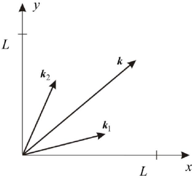
Figure 1: Wave vectors for three interacting Fourier components (plane waves) in the spatial domain $L\times L$.

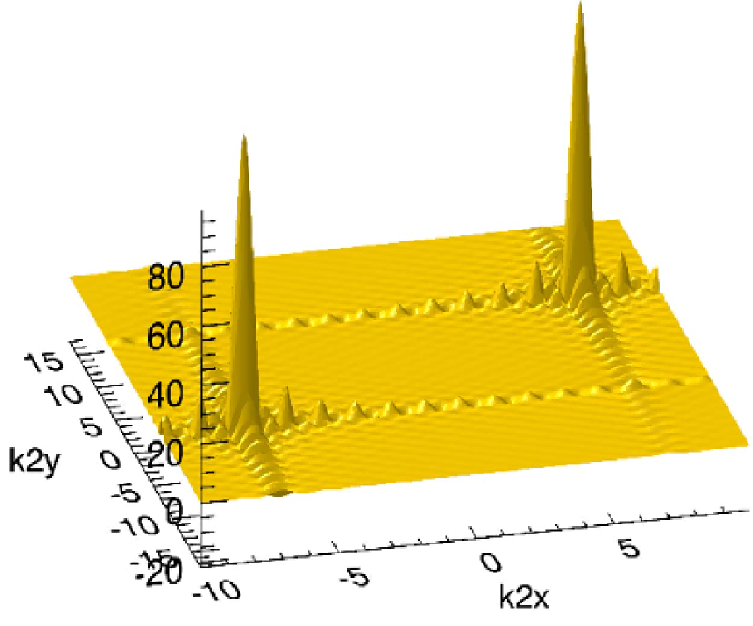
Figure 2: Overlap integral as a function of $\bm{k}_{2}$ for a fixed value of $\bm{k}_{1}$.

We notice that the width of the wave number uncertainty, $\Delta k_{x}$, defined by the zero crossings of the sinc-function, $\Delta k_{x}L/2=2\pi$, depends on the interaction area side length, $L$. The effect on the turbulence power spectrum by this spectral window is illustrated in Figure 3, which compares a computer simulation with and without the effect of the finite interaction area. The suppression of odd numbered ‘harmonics’, as observable from Figure 3b, will be explained in the following.

Figure 3 shows the development of the spectrum of an initial signal consisting of a single spatial frequency of $50\,m^{-1}$ after several cycles of triad interactions. Figure 3a presents the case of a large measurement volume. The resulting high spatial bandwidth and narrow spectral band width does not cause interference between the conversion efficiency and the harmonic frequency peaks. Figure 3b shows the case of a small measurement volume. The sinc-function spectral window in this case interferes with the conversion efficiency.

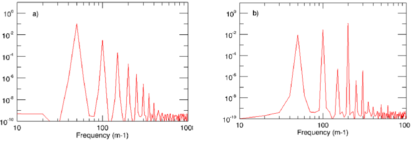
Figure 3: Computer simulation of the development of the spectrum of an initial signal consisting of a single spatial frequency of $50\,m^{-1}$. Figure 4(a): Large interaction volume, high spatial bandwidth which does not interfere with the conversion efficiency. Figure 4(b): Small interaction volume, the sinc-function spectral window influences the conversion efficiency.

VI Cascaded delays – time evolution of spectra

As described above, energy can be passed to a mode with wave vector $\bm{k}$ by modal interactions with modes with wave vectors $\bm{k}_{1}$ and $\bm{k}_{2}$. The potential mismatch between spatial and temporal frequencies allowed for delays in the interactions to occur between velocities sampled at different times. Each interaction thus develops with a characteristic time, which depends both on the magnitude of the Fourier components (which is determined by the signal strength), the spectral bandwidth and the overlap efficiency factor, which depends on the size of the finite experimental region.

However, the interaction time also depends on the number of time steps needed to go from $\bm{k}_{1}$ and $\bm{k}_{2}$ to $\bm{k}$. Thus, the number of delays in each modal interaction is proportional to $1+|j_{1}-j_{2}|$, where the initial value 1 accounts for the first interaction process and $j_{1}$ and $j_{2}$ are two wavenumber indices (integers) numbering the orders of the harmonics of the wave vectors interacting to produce the resulting peak in wavenumber space.

The cascaded delay in time space is proportional to the sum of time delays. Let us give a couple of examples, where we consider individual modal interactions in $k$-space. We consider the presence of only one spatial input frequency component, $k_{0}$, and look at a few simple cascade processes for the formation of harmonics. Three different low order cascade processes are illustrated in Figure 4.

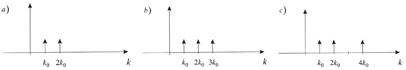
Figure 4: (a) Frequency doubling. (b) Frequency tripling. (c) Frequency quadrupling.

Frequency doubling: $k_{0}\Rightarrow 2k_{0}$
In this example, $k_{1}=k_{2}$, hence $j_{1}=j_{2}$ and there is only one delay, $1+|j_{1}-j_{2}|=1$.

Frequency tripling: $k_{0}+2k_{0}\Rightarrow 3k_{0}$
Here $k_{1}=k_{0}$ and $k_{2}=2k_{0}$. Thus $1+|j_{1}-j_{2}|=2$. But $k_{2}=2k_{0}$ must be created first resulting in a total cascade delay of 3. Moreover, in a realistic situation, $k_{1}$ and $k_{2}$ would be quite different in size, resulting in a less efficient spatial overlap and interaction as described above.

Frequency quadrupling: $2k_{0}+2k_{0}\Rightarrow 4k_{0}$
Here $k_{1}=2k_{0}$ and $k_{2}=2k_{0}$. $j_{1}=j_{2}$, so there is only one delay in this interaction, $1+|j_{1}-j_{2}|=1$. But $2k_{0}$ must be created first, resulting in a total cascade delay of 2. Thus, the fourth harmonic would be created earlier and more efficiently than the third harmonic.

It should be noted here that the actual processes are difficult to isolate and that experiments to unveil these processes therefore are often sensitive to experimental conditions, including initial and boundary conditions (which is also well known to be the case for the differential equations that govern the flow). Other effects that further complicate the interactions are the multiple lobes in the window function, the fact that the window function is in general not rectangular and that the window is likely to fluctuate wildly in time and space. Nevertheless, we have been able to isolate this effect to a reasonable degree and observe the developments of the delayed interactions, as described in more detail in the following section.

VII Experiments and numerical simulations

Our simple analysis allows us to estimate the duration of individual modal interaction processes and the total delay in a process involving a number of cascade steps. We have illustrated these results in two ways. In one study [15], we measured the development of the velocity power spectrum using a hot-wire anemometer in the approximately laminar core of a large free jet in air into which we injected a single large mode upstream. By measuring the power spectrum at several downstream locations, we could follow the time development of the spectrum and the appearance of the first higher harmonics generated by the nonlinear term in the Navier-Stokes equation. As can be seen in Figures 5 and 6, we used vortex shedding behind a rod with a rectangular cross-section placed across the jet to inject a narrow band oscillation which can represent a single oscillating mode close to the jet exit. The jet exit had a contraction ratio of $2.4:1$ and an exit diameter of $100\,\mathrm{mm}$. The jet was run at a jet exit velocity of $1.6\,\mathrm{ms}^{-1}$. This produced a sufficiently large laminar jet core to be able to serve well as an open wind tunnel test section. The rectangular rod had a cross-section of $2\,\mathrm{mm}\times 10\,\mathrm{mm}$ and thus significantly smaller dimensions than the jet exit. The rod length was $300\,\mathrm{mm}$, corresponding to three jet exit diameters and the rod was placed to cover with good margin the jet nozzle extent across the exit diameter. The rod was positioned $1\,\mathrm{mm}$ from the nozzle and across the jet exit so that it was passing through the jet centerline.

The sharp edges of the rectangular cross-section enabled vortex shedding with a sufficiently distinct base frequency to be able to trace the downstream development of the first and subsequent harmonics. This effect turned out to be most distinguishable in the measurements when the longest dimension ($10\,\mathrm{mm}$) of the rod cross section was aligned with the jet centerline. A single component hot-wire with a PicoScope to monitor the live spectral frequency content was used to select the optimal flow setting, measurement positions and to acquire the end result. This resulted in acquisition of the above described flow setting in ten positions along the downstream direction with $1\,\mathrm{mm}$ spacing, of which only the downstream positions $1\,\mathrm{mm}$, $5\,\mathrm{mm}$ and $10\,\mathrm{mm}$ are shown herein. The most upstream measurement point was placed $0.5\,\mathrm{mm}$ to the side away from the edge and the wake of the rod, see Figure 5. Further detail about this experiment can be found openly available [15].

The first spectrum, Figure 6a, shows the measured power spectrum $1\,\mathrm{mm}$ downstream from the rod where only the fundamental oscillation is present. Figure 6b shows the spectrum $5\,\mathrm{mm}$ downstream and Figure 6c the spectrum $10\,\mathrm{mm}$ downstream. 100 measured spectra have been averaged for each downstream position. The development of the cascade process is clearly visible. Knowing the velocity as a function of downstream position, we can calculate the convection time and thereby find the time history for the modal interactions [15].

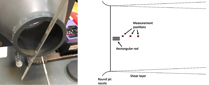
Figure 5: (Left) Picture and (Right) sketch of the simple experimental setup used to isolate the interactions resulting from a distinct frequency shed off from a rectangular rod. The jet was large compared to the rod, such that the laminar core of the jet could create an environment similar to an open wind tunnel test section. A single component hot-wire (as seen in the left figure) was used to trace the downstream development from the initial single frequency injected by the rectangular rod.

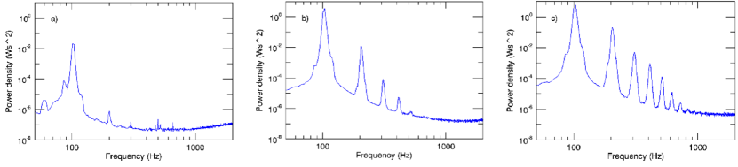
Figure 6: Measured velocity power spectra with increasing downstream positions from left to right. a) $1\,mm$, b) $5\,mm$ and c) $10\,mm$ downstream.

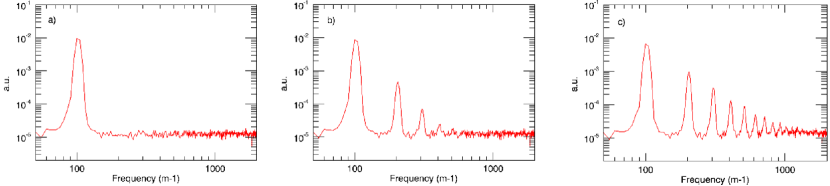
Figure 7: Computed velocity power spectra at increasing time from left to right. The downstream development time has been chosen to approximately match the downstream developments displayed in Figure 6.

In a second paper [7], we show results of a computer calculation of a one-dimensional projection of the Navier-Stokes equation. We have implemented a one-dimensional version of the Navier-Stokes equation [16] in a program that can be executed on a laptop PC in a few minutes. By neglecting the direction of the velocity vector and only considering the velocity magnitude at a point as a function of time, the system of equations reduces to one dimension so that it is numerically solvable. The one-dimensional solution allows us to compute the kinetic energy and the turbulent structure functions directly from the Navier-Stokes equation without any additional assumptions except for the pressure term, which would require either a full three-dimensional solution for the whole flow field or a model for the pressure fluctuations [16]. We are, among many other things, able to simulate the time development of a velocity power spectrum consisting of a low intensity von Kármán-type turbulence to which we added a single low frequency mode.

In Figure 7, we show the development of a single Fourier mode in the same laminar jet core flow as described above and in Figure 5 and 6. Instead of a computer-generated oscillating time trace, we used the time trace actually measured near the rod as input (the same position and same velocity trace as in Figure 6a) and processed the downstream development of this time trace using our Navier-Stokes simulator [7].

Thus, the first plot should be identical to the measured one. (The slight differences in the initial spectra are due to the somewhat different filter settings and window functions of the PicoScope used for the measured spectra and the fast Fourier transform (FFT) settings used for the computations). The following plots show the velocity power spectrum computed by the Navier-Stokes simulator based on an average of 20 measured time traces. This should be held up against the ones measured downstream where the convection time has allowed the flow to develop. One clearly sees the effect of the cascaded delays on the development of the spectrum and the sequence of appearance of the first harmonics.

VIII Conclusions

The triad interactions most often analyzed assuming infinite spatial velocity fields and an analytical Fourier integral resulting in delta function phase match conditions present a too simplified description of triad interactions in the case of real measured velocity records. We analyzed how measured velocity records having finite spatial and temporal domains and finite digital sampling rates modify and expand the description of modal interactions and the development of the power spectrum of the flow.

The finite spatial and temporal domain of the velocity field creates a spectral window for the triad interactions, which introduces a spectral broadening effect and facilitates local triad interactions. Furthermore, the limited spatial domain influences the efficiency of the Fourier component overlap, which alters the shape of the generated spectrum. We illustrate the dynamic evolution of the spectra by estimating the time constant for each triad interaction and considering the sequence of the interactions needed to create a harmonic frequency. This process illustrates the so-called spectral cascade by considering which interactions must precede the following with the associated delay. The experiments and simulations lend strong support to this picture as well.

Finally, we quoted some results from two previous papers. These examples show good agreement between a measurement in a free jet in air into which a single Fourier component is injected, for instance by a vortex shedding, and a computation of the time development of the same velocity time trace by a projection of the forces in Navier-Stokes equation onto the instantaneous velocity direction.

As also discussed in the companion paper (Part 1) [1], these investigations have resulted in a better understanding of triad interactions in the case of digitally sampled velocities with finite temporal and spatial measurement domains. We have also illustrated the effects of practical experiments on the processes participating in the non-linear triadic interactions and energy transfer between scales in turbulence generation and decay.