MeMo: Meaningful, Modular Controllers via Noise Injection
Abstract
Robots are often built from standardized assemblies, (e.g. arms, legs, or fingers), but each robot must be trained from scratch to control all the actuators of all the parts together. In this paper we demonstrate a new approach that takes a single robot and its controller as input and produces a set of modular controllers for each of these assemblies such that when a new robot is built from the same parts, its control can be quickly learned by reusing the modular controllers. We achieve this with a framework called MeMo which learns (Me)aningful, (Mo)dular controllers. Specifically, we propose a novel modularity objective to learn an appropriate division of labor among the modules. We demonstrate that this objective can be optimized simultaneously with standard behavior cloning loss via noise injection. We benchmark our framework in locomotion and grasping environments on simple to complex robot morphology transfer. We also show that the modules help in task transfer. On both structure and task transfer, MeMo achieves improved training efficiency to graph neural network and Transformer baselines.111Correspondence to megantj@mit.edu. Code can be found at https://github.com/MeganTj/MeMo.
1 Introduction
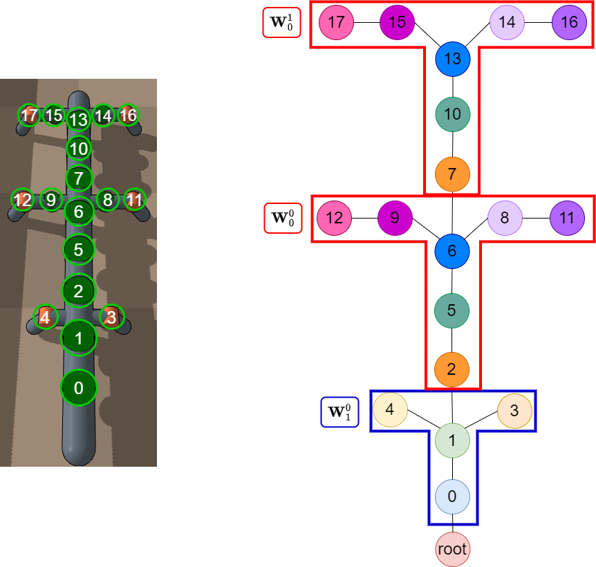
Consider the following scenario: A roboticist is designing a robot with 6 legs, such as the one seen in the left image of Fig. 1, and has trained a standard neural network controller with deep reinforcement learning (RL) to control the actuators circled in green. However, after more testing, they realize that the design of the robot needs to be extended with another pair of legs to support the desired amount of weight. Even though the new 8 leg robot is still composed of the same standard assemblies, the roboticist is unable to reuse any part of the 6 leg robot’s controller. While many works [1, 2, 3] have studied structure transfer, or transferring neural network controllers to different robot morphologies, these works take a purely data-driven approach of training a universal controller on a dataset representative of the diversity and complexity of robots seen in testing. In contrast, we desire to learn transferable controllers from only a single robot and environment, obviating the requirement for a substantial training dataset and resources to perform multi-task RL. Our experiments demonstrate that state-of-the-art approaches for transferring control to environments with incompatible state-action spaces struggle to generalize in this highly data-scarce setting.

Motivated by the above scenario, we propose a framework, MeMo, for pretraining (Me)aningful (Mo)dular controllers that enable transfer from a single robot to variants with different dimensionalities. Learning transferable modules from a single robot trained on a single task is challenging, even when we focus on transfer among robots with similar global morphologies. The key insight MeMo leverages is that a robot is built from assemblies of individual components, such as the leg of a walking robot or the arm of a claw robot. These assemblies are specified by a domain expert who is able to account for the constraints imposed by the robot’s hardware implementation in their specification. Given this information, MeMo learns assembly-specific controllers, or modules, responsible for coordinating the individual actuators that comprise a given assembly, which are coordinated by a higher-level boss controller. As we are able to reuse the modules when transferring to a robot built from the same assemblies, the problem of learning a controller for a different morphology boils down to learning the coordination mechanics among assemblies, rather than having to coordinate at the granular level of individual joints. Returning to the 6 leg robot in Fig. 1, we see that the robot is comprised of multiple “leg" and “body" assemblies, circled in red and blue respectively in the right image. Module parameters are shared between assemblies of the same type, providing multiple training instances that help our modules generalize. After training the modules with MeMo, the “leg" and the “body" modules can then be reused to speed up the training of a different robot’s controller, such as an 8 leg robot.
To achieve this improved training efficiency, a key challenge is to balance the labor between the boss controller and the modules. In one direction, to prevent the modules from becoming too robot-specialized, we introduce information asymmetry into our architecture, where the modules are limited to seeing the local observations of the actuators that belong in the module. In the other direction, controlling the assembly through the module must be simpler than controlling the assembly directly, since otherwise there is no benefit to this new architecture. This is achieved by a new modularity objective (Section 2) that forces the modules to capture as much of the coordination mechanics within a subassembly as possible, given limited local observations. In practice, we use noise injection (Section 3.1) to optimize the new objective simultaneously with standard behavior cloning loss.
To evaluate the transferability of the learned module, we apply MeMo in locomotion and grasping domains. We design two types of transfer: generalizing to more complex robot structures and to different tasks. When transferring model weights from a simpler agent, we show that MeMo significantly improves the sample efficiency of performing RL on more complex agents. We compare our framework with NerveNet, an alternative approach for one-shot structure transfer [4, 5], and MetaMorph [3], an approach for learning universal controllers. Our experiments show that MeMo either exceeds or matches NerveNet and MetaMorph’s training efficiency during transfer, as the message-passing policies are prone to overfitting during pretraining.
2 Motivation for Modularity Objectives
Our goal is to maximize the extent to which the assembly-specific modules take responsibility for the behavior of the robot. In this section, we formalize the objectives that our training pipeline should achieve. Given an expert controller F, one can train a modular controller, consisting of a higher-level B(oss) module that sends a signal to each of the W(orker) modules, to mimic F’s behavior using the standard behavior cloning objective. Let B be parameterized by and W be parameterized by . For simplicity, this section assumes that there is a single W module.
Definition 2.1.
Behavior Cloning Objective. For a system with states , the modular policy whose output is imitates the expert monolithic policy F.
| (1) |
The behavior cloning objective ensures that the composition of modules can perform the desired task, but it is not enough to ensure that the worker module is useful. In software engineering, a component is most useful if it can provide a narrow interface to a rich set of functionality. In the context of modularity, this is analogous to W giving B only a few degrees of freedom to control the system’s outputs; otherwise, a module W that gives B full control over the actuators will leave W with no real responsibility for the robot’s behavior. Then, when W is used with a new robot or for a slightly different task, B needs to relearn all the details of how to control the output for that new setting.
For example, consider a robot arm with 5 degrees of freedom that controls a lever in Fig. 2. An ideal worker module would take as input a signal corresponding to the desired angle of the lever and would be responsible for coordinating the signals to the five actuators to achieve the lever’s desired position. This would mean that if we want to reuse W in controlling two arms, the new boss B’ will only have to learn how to coordinate the two angles, and not all 10 actuators.

In practice, though, forcing the interface between B and W to be a one dimensional vector makes the optimization problem very difficult. Instead, our approach will be to use a larger vector as the interface between the two modules, but introduce an additional optimization objective. Intuitively, the interface is effectively narrow when B’s signal can be decomposed into a small set of dimensions that result in greater variance in W’s output and a much larger set of dimensions that do not cause significant perturbations in W’s output. In other words, the null space of W’s Jacobian would be higher-dimensional, meaning that W has a greater tolerance for error in B’s signal that fall in the directions of the null space. To encourage W to be less sensitive to perturbations in B’s signal, we minimize the distance between , where is a noise vector, and .
Definition 2.2.
Invariance to Noise Objective. Let be a noise vector. The difference between the result of applying W on the distorted input and on the undistorted input is . As a new distortion to is added on each epoch, we average the difference over the added noise.
| (2) |
In practice, we sample from a Gaussian distribution with and , where . In Section 5.3, we demonstrate that our invariance to noise objective is the critical component in our framework that yields positive transfer benefits. In Section 5.4, we show that optimizing the noise invariance objective reduces the effective dimensionality of B’s signal.
3 Method
We describe our approach MeMo, an algorithm for learning reusable control modules. In Section 3.1, we show that the modularity objectives can be optimized with noise injection. In Section 3.2, we extend our formulation to systems with more than one module and detail our training pipeline.
3.1 Objective
We propose to optimize both modularity objectives simultaneously with noise injection.
Definition 3.1.
Noise Injection Objective. Here, can be viewed as “injected noise."
| (3) |
The noise injection loss can be decomposed as follows:
| (4) |
See Appendix A.4 for the derivation of the decomposition. Without the last term, which we call the product term, noise injection is equivalent to the sum of Eq. 1 and 2. Analyzing the product term further, by the Mean Value Theorem, for , where denotes the Jacobian of W with respect to B’s output and is the line segment with and as endpoints. Applying the expectation over the noise:
| (5) |
Note that depends on the value of , so it cannot be pulled out of the expectation. However, in practice, we expect that . This implies that , making the product term negligible. Empirically, in Fig. 3, we show that this product term indeed becomes much smaller than the sum of the two modularity objectives as training proceeds.

3.2 Modular Architecture and Training Pipeline
Modular Architecture. Although thus far we have only a single module W, a robot is often comprised of multiple modules controlling physical assemblies that are common among different morphologies. Formally, we assume that we are given a partitioning of an agent’s joints . We design a modular policy composed of a boss controller B that outputs intermediate signals to neural network modules that decode actions. Each element of the partition, e.g. a subset of actuators, is a module instance of type , which we denote as . In total, there are modules. Modules of the same type share the module parameters, yet each instance will receive a different message from B. We detail our architecture further in Appendix A.3.
Training Pipeline. To train our modules, inspired by previous works that combine RL and IL [6, 7, 8], we first train F using RL. During the RL stage, we use proximal-policy optimization [9] to train actor-critic controllers. The critic is a MLP, whereas the actor is a standard MLP when training the expert controller and a modular architecture when transferring pretrained modules. Once F is trained, we train a modular policy with IL via DAgger [10], with noise injected into ’s output. At each iteration of DAgger, we sample a trajectory from . F provides the correct action to each , and is aggregated into the full dataset . To optimize the objective defined in Section 3.1, we minimize . We derive a decomposition of the negative log likelihood loss with noise injection into the modularity objectives in Appendix A.5. After transferring the modules to a new structure or task, we perform RL to retrain B or finetune the architecture end-to-end. Our pipeline is summarized in Fig. 4. Appendix A.6 details our RL and IL hyperparameter settings.

4 Related Work
Our work relates to modular controllers and structure transfer. Related works in noise injection, multi-robot RL, and hierarchical RL are discussed further in Appendix A.11.
Modular Controllers. Our work relates to prior works that train modular policies for robot designs. [11] learns neural network policies that are decomposed into “task-specific" and “robot-specific" modules and performs zero-shot transfer to unseen task and robot-specific module combinations. [1] coordinates modular policies shared among all actuators via message passing. [12] uses a GNN to internally coordinate between part-specific nodes with shared module parameters between nodes corresponding to the same part. [13] proposes the Dynamic Graph Network to control self-assembling agents, consisting of modules that are shared across agents.
Structure Transfer. In the hierarchical RL setting, [14] uses imitation learning to train policies that represent long-horizon behavior and improve sample efficiency when transferred from simple to complex agents. [15] transfers policies to robots with significantly different kinematics and morphology by defining a continuous evolution from the source to the target robot. Previous works use message-passing policy architectures to generalize across morphologies [1, 4, 5]. In the multi-task setting [2] proposes Transformers as policy representations that remove the need for multi-hop communication. [3] scales Transformer-based policies to larger and more diverse datasets of robots.
5 Experiments
With our experiments, we seek to answer four questions. 1) Do the modules produced by MeMo generalize when transferred to different robot morphologies and tasks? 2) When pretraining modular controllers with imitation learning, does the Gaussian noise injection help? 3) In the pretraining phase, why do we use imitation learning rather than injecting noise in reinforcement learning? 4) How does our modularity objective yield better representations of the actuator space? We answer question 1) in Sections 5.1 and 5.2, 2) and 3) in Section 5.3, and 4) in Section 5.4.
5.1 Transfer Learning
We benchmark our framework on two types of transfer: structure and task transfer. While our framework is designed primarily for structure transfer, we use task transfer experiments as an additional means of evaluating the quality of the learned representations. For the locomotion experiments, we perform experiments on the tasks introduced in RoboGrammar [16] with training statistics computed as the average reward across 3 runs, with standard deviations indicated by shaded areas. For the grasping domain, we construct object-grasping tasks using the DiffRedMax simulator [17] and compute training statistics as the average reward across 5 runs. Additional details on the reward functions used are in Appendix A.9. We visualize train and test robot morphologies for structure transfer in Fig. 5 and the train and test tasks for task transfer in Fig. 17.
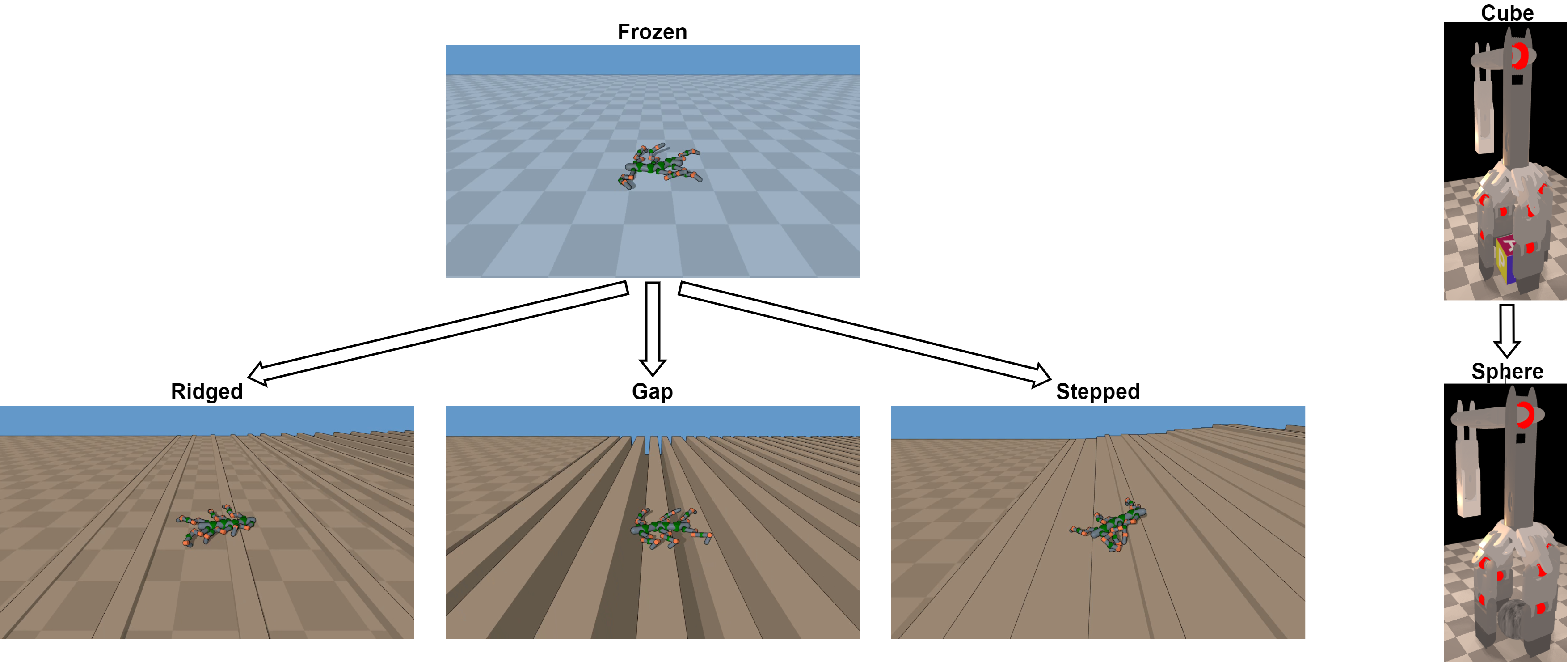
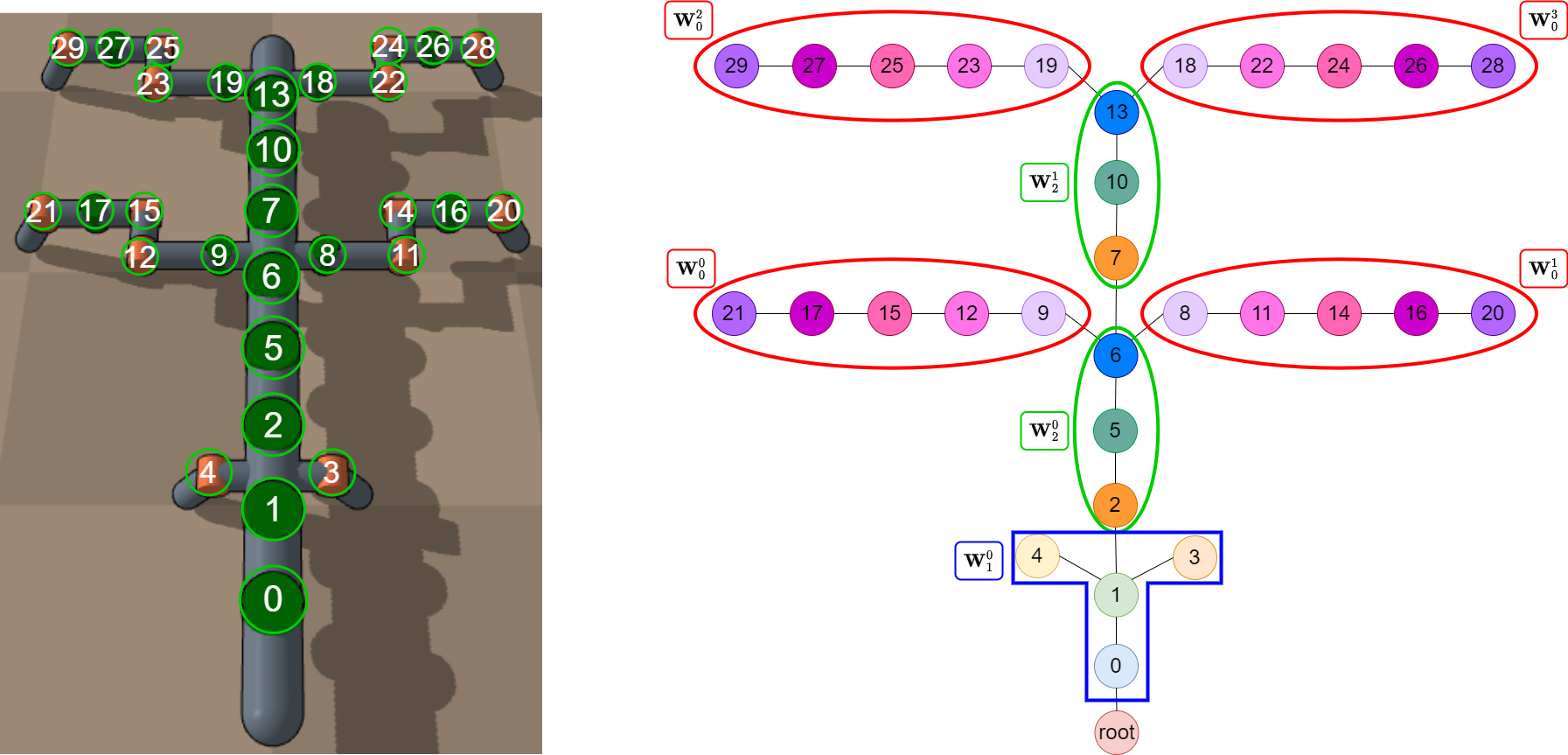
Locomotion. We design three structure transfer tasks in the locomotion domain, in which the goal is to move as far as possible while maintaining the robot’s initial orientation. The starting morphologies are the 6 leg centipede robot, the 6 leg worm robot, and the 6 leg hybrid. The 6 to 12 leg centipede transfer demonstrates scalability to transfer robots with many more modules than seen in training. The 6 to 10 leg worm shows that MeMo generalizes with only 1-2 instances of the same module seen in training. The 6 and 10 leg hybrid robots involve three types of modules, demonstrating scalability to more complex training robots. For task transfer, we transfer policy weights pretrained on a 6 leg centipede locomoting over the Frozen Terrain to three terrains that feature obstacles or climbing.
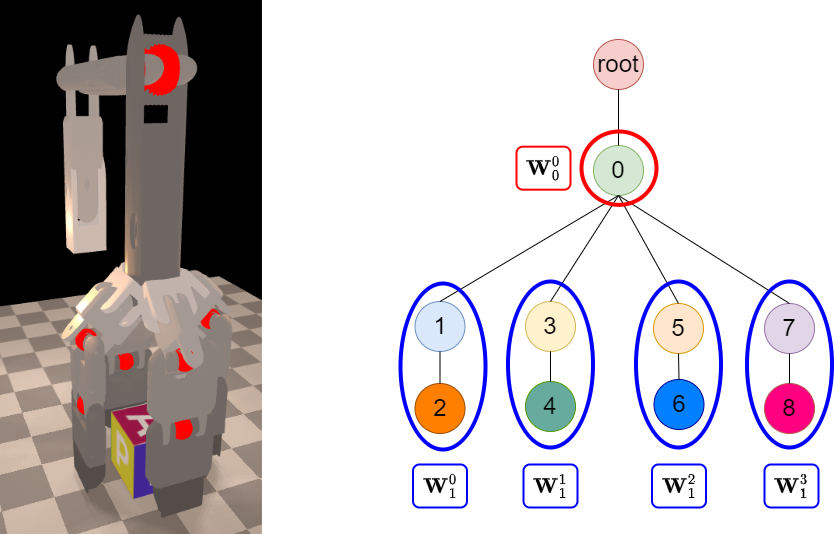
Grasping. In grasping, the goal is to grasp and lift an object as high as possible. We design a grasping robot consisting of an arm that lifts a claw grasping a cube. The structure transfer is from a 4 finger to a 5 finger claw. For task transfer, we transfer policies trained to control the 4 finger claw grasping a cube to the same robot grasping a sphere of similar size and weight.

Baselines. We compare MeMo to MLP and modular policies trained from scratch as well as pretrained NerveNet [4, 5] and MetaMorph [3] baselines. NerveNet takes as input the underlying graph structure of the agent, where the nodes are actuators and edges are body parts. The graph structures of the train morphologies are detailed in Appendix A.13. For MetaMorph, a Transformer-based approach, we convert the global observations and local observations for each actuator to a 1D sequence of tokens. Full training details and state space descriptions are included in Appendix A.6 and A.7 respectively.
-
•
RL (MLP): For structure transfer, due to the change in the observation space, we train a 2 layer MLP policy from scratch with RL. In task transfer, we use a MLP pretrained with RL on the original task and finetune it on the test task. For a fair comparison, we use the same architecture size as the modular architecture’s boss controller and replace the modules with a linear layer decoder.
-
•
RL (Modular): For structure transfer, we train the modular architecture, discussed in Section 3.2, from scratch with RL. In task transfer, we use the modular architecture pretrained with RL on the training task and finetune both the modules and the boss controller on the test task. The inclusion of this baseline allows us to isolate the effect of the modular architecture from the pretraining and noise injection components of MeMo.
-
•
Pretrained NerveNet-Conv: We use the NerveNet network architecture proposed by [4], consisting of an input network for encoding observations, a message function , an update network , and an output network for decoding. As in [4], and are MLPs. In the convolutional [18] variant, is the identity function and is a weight matrix. During RL, we fix in a similar manner as fixing the modules in MeMo, which improves NerveNet-Conv’s performance.
-
•
Pretrained NerveNet-Snowflake: Snowflake [5] is a state-of-the-art approach for training GNN policies that scale to high-dimensional continuous control. Their method involves fixing parts of the NerveNet architecture to prevent overfitting during PPO. Empirically, they find that fixing results in the best performance on MuJoCo tasks. We follow the same parameter fixing as Snowflake. As in Snowflake, we parameterize and as MLPs and the update function as a GRU. We use a weight matrix for .
-
•
Pretrained MetaMorph: MetaMorph [3] is a Transformer-based approach for learning a universal controller over a large collection of robot morphologies. We adopt MetaMorph’s Transformer architecture for the policy network, which adds learned positional embeddings before processing the input sequence with a Transformer encoder. As our domains lack exteroceptive observations, we directly decode Transformer encodings to controller outputs. The Transformer policy is finetuned during RL.
5.2 Results


The generalization ability of MeMo on structure transfer is shown in Fig. 6. On all structure transfer tasks, MeMo outperforms the message-passing baselines. On the 12 leg centipede and the 10 leg hybrid, not only is MeMo 2 more sample efficient than the best baseline, but it also converges to controllers with significantly better performance than any baseline. On the 10 leg worm, MeMo outperforms all baselines in terms of training efficiency and achieves a comparable final performance as NerveNet-Conv. MeMo also outperforms all baselines on the 5 finger claw. We note that the worm transfer task is easier for GNN models, because the coordination of the shorter legs and body joints is naturally captured with multi-hop communication. MetaMorph struggles with locomotion tasks, due to the high dimensionalities of the transfer robots.
The results of MeMo on task transfer are shown in Fig. 7. As transferring from the Frozen to the Ridged, Gap, and Stepped Terrains requires the robot to overcome obstacles unseen in the Frozen Terrain, we load the pretrained boss controller and finetune MeMo end-to-end. Results (Fig. 7) show that on all test tasks, MeMo achieves improved training efficiency compared to MetaMorph and to pretrained MLP and modular architectures. MeMo achieves comparable performance on the Ridged and Gap Terrains and outperforms the NerveNet baselines on the Stepped Terrain, which requires the robot to climb up steps whereas the training terrain is flat. MeMo also has improved training efficiency and final performance in the grasping domain when transferring from grasping a cube to a sphere. The pretrained NerveNets struggle to coordinate the arm and claw components, resulting in high variance across different random seeds.
5.3 Ablation Study
Sum of Modularity Objectives. We answer the question of why we choose to optimize the noise injection objective rather than the sum of the modularity objectives directly. We evaluate the sum of Eq. 1 and 2 between networks trained with the noise injection objective and those trained with the sum in Table 1. Using 100 sampled trajectories from the expert controller, we average the resulting sum of objectives over 1000 epochs, with different sampled noise on each epoch. Our results demonstrate that optimizing the noise injection objective converges to better solutions.
| Morphology | Noise Injection | Dual Loss |
|---|---|---|
| Centipede | -33.518 | -33.115 |
| Worm | -39.295 | -35.896 |
| Hybrid | -30.536 | -27.849 |
| Claw | -8.215 | 0.279 |
Noise Injection Objective. The key to the success of MeMo is the introduced noise injection (NI) objective which encourages proper responsibility division among the pretrained boss controller and modules, enabling the modules to improve training efficiency when reused. We conduct an ablation study to verify this technique by experimenting on a special setting, “transferring" the controller to the same robot structure and task, a 6 leg centipede traversing a Frozen Terrain. During transfer, we reuse and freeze the pretrained modules and retrain the boss controller from scratch. With the pretrained modules from MeMo, the boss controller will be retrained much more efficiently because it only needs to take partial responsibility for the control job. We compare our method to three baselines:
-
•
MeMo (no NI): We pretrain the modular architecture end-to-end without noise injection. This ablation is equivalent to MeMo without noise injection.
-
•
MeMo (L1): During pretraining, we replace the injected noise with L1 regularization on B’s output that encourages sparsity in its signal. We weigh the regularization term by a hyperparameter and report results with the best .
-
•
MeMo (L2): During pretraining, we replace the injected noise with L2 regularization on B’s output and report results with the best weight on the regularization term.
-
•
MeMo (Jacobian): As an alternative to noise injection, we penalize the norm of the module’s Jacobian using the method described in [19].
In addition, we add the training curve of RL (Modular) as a reference. The results (Fig. 8) show that MeMo yields a significant improvement in training efficiency over all ablations.
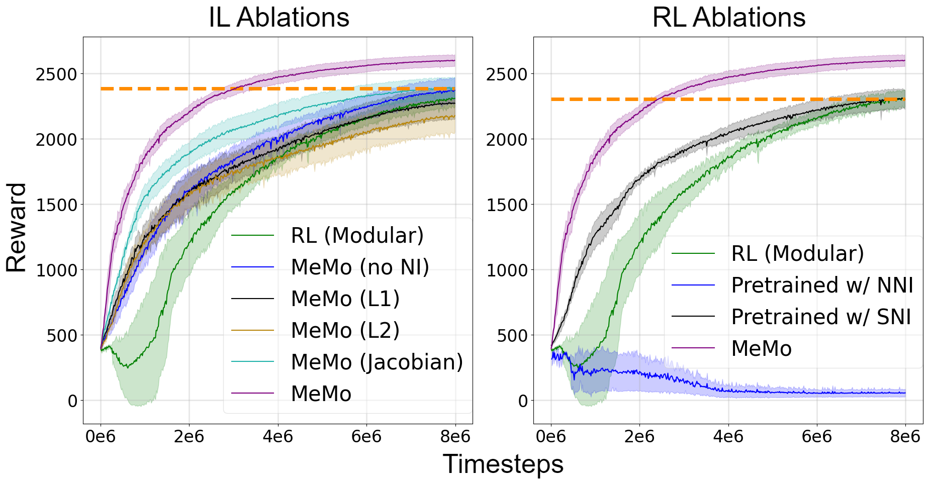
Imitation Learning. We now answer the second question of whether imitation learning is necessary to pretrain modules with Gaussian noise injection. The results of using noise injection in reinforcement learning to pretrain modules is shown in Fig. 8. Note that we refer to IL ablations as experiments where modules are first pretrained with imitation learning, and subsequently, the boss controller is reinitialized and retrained with RL to test the improvement in sample efficiency. RL ablations involve the second RL phase, but the pretraining stage is done with RL as well. In addition to training the modular architecture from scratch, we experiment with two methods of injecting noise during RL. The first is naive noise injection (NNI), where we inject noise into B’s output when sampling rollouts and computing policy gradients. For the second, we adopt the Selective Noise Injection (SNI) technique proposed by [20] for applying regularization methods with stochasticity in RL. SNI stabilizes training by sampling rollouts deterministically and computing the policy gradient as a mixture of gradients from the deterministic and stochastic policies. However, even with SNI, the pretrained modules do not improve training efficiency.
5.4 Analysis
We examine how the noise injection objective forces the modules to learn a better representation of the actuator space. As discussed in Section 2, the trajectories produced by a successful policy often lie on a much lower-dimensional manifold than the actuator space. Each dimension of the manifold can be interpreted as an individual skill that the policy has learned. We can measure the dimensionality of the modules’ mapping by looking at the Jacobian matrix of the worker modules with respect to the boss’s signal. The trajectories outputted by a policy can likely be captured by a few dimensions of high variance corresponding to a small set of large singular values in addition to a much larger set of dimensions of lower variance corresponding to relatively small singular values.
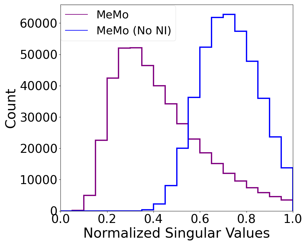
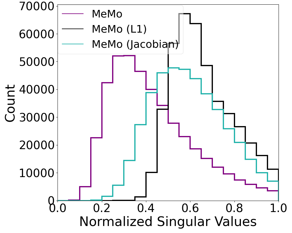
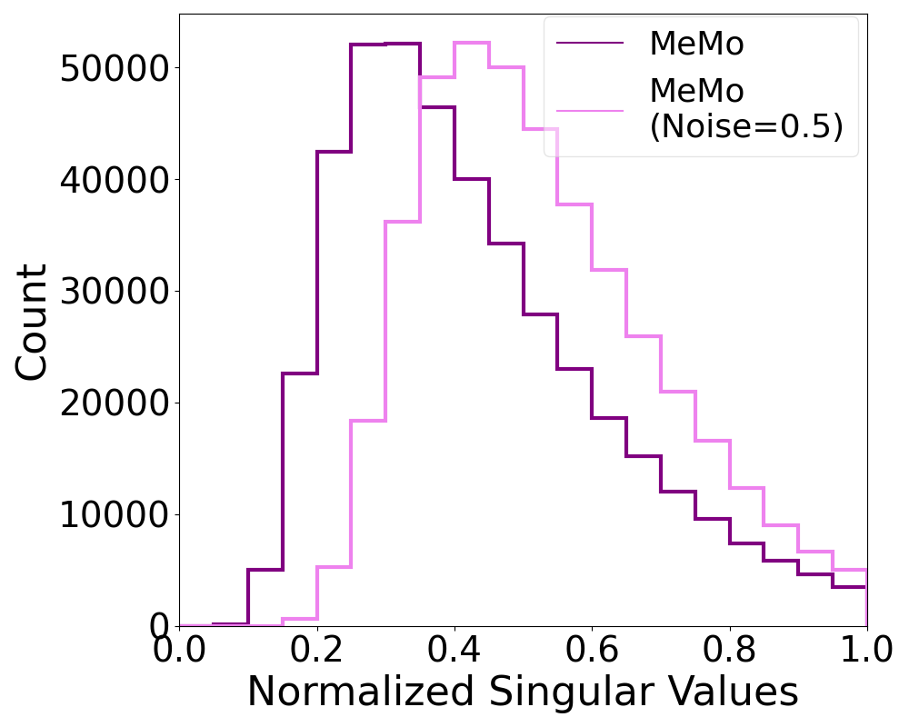
We visualize this effect by 1) computing the Jacobians at the trajectory input states of a successful policy and 2) normalizing the singular values of each Jacobian by its largest singular value and plotting the resulting values in the [0, 1] range. We expect that a module that optimizes the invariance to noise objective will have only a small number of large singular values, with the rest being close to zero. Conversely, modules that do not produce a low-dimensional manifold would have more singular values of similar magnitude, resulting in the distribution’s mass clustering close to 1. We verify this intuition by sampling 100 trajectories from an expert controller for the 6 leg centipede shown in Fig. 1. We compare the plots of the normalized singular values between MeMo and MeMo without noise injection in Fig. 9. Without noise injection, the majority of the values are close to 1. At the other extreme, with MeMo, the values are highly clustered to the left, implying that most singular values are much smaller than the biggest singular value. We plot the singular value distributions of additional MeMo ablations in Appendix A.12.
6 Conclusion
In this paper, we propose a modular architecture for robot controllers, in which a higher-level boss controller coordinates lower-level modules that control shared physical assemblies. We train the architecture end-to-end with noise injection, which ensures that the lower-level modules do not overrely on the boss controller’s signal. In locomotion and grasping environments, we demonstrate that our pretrained modules outperform both GNN and Transformer-based methods when transferring from simple to complex morphologies and to different tasks. We ablate components of MeMo and demonstrate that the entire framework is necessary to achieve these generalization benefits.
Acknowledgments and Disclosure of Funding
MT is supported by the National Science Foundation (NSF) under Grant No. 2141064. MT was also additionally supported by the MIT Stata Presidential Fellowship. This work greatly benefited from discussion with colleagues in the MIT Computational Design and Fabrication Group and MIT Computer-Aided Programming Group. Any opinion, findings, and conclusions or recommendations expressed in this material are those of the authors(s) and do not necessarily reflect the views of the funding entities.
References
- [1] W. Huang, I. Mordatch, and D. Pathak, “One policy to control them all: Shared modular policies for agent-agnostic control,” in Proceedings of the 37th International Conference on Machine Learning, 2020.
- [2] V. Kurin, M. Igl, T. Rocktäschel, W. Boehmer, and S. Whiteson, “My Body is a Cage: The Role of Morphology in Graph-Based Incompatible Control,” in International Conference on Learning Representations, 2021.
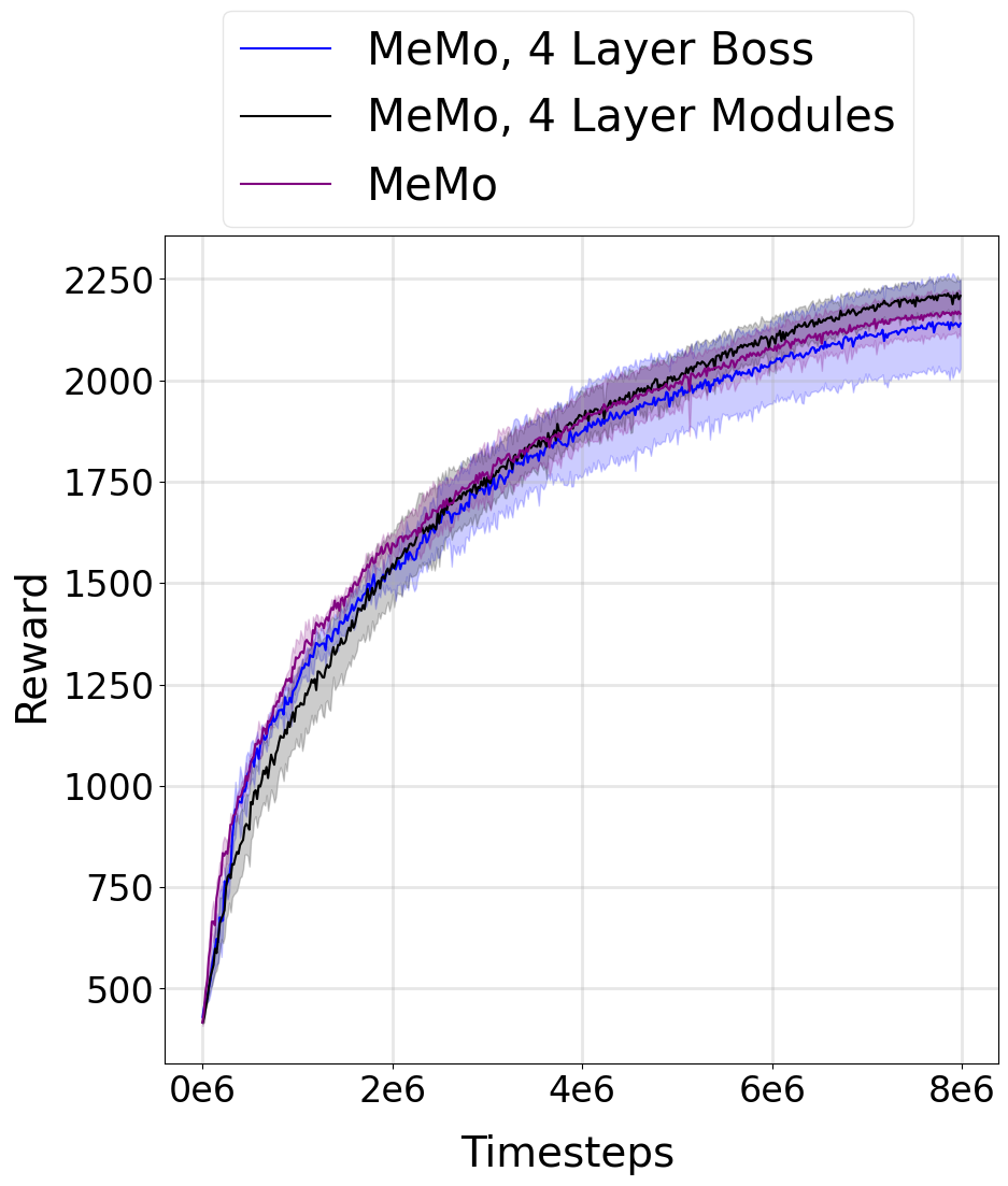
- [3] A. Gupta, L. Fan, S. Ganguli, and L. Fei-Fei, “MetaMorph: Learning Universal Controllers with Transformers,” in International Conference on Learning Representations, 2022.
- [4] T. Wang, R. Liao, J. Ba, and S. Fidler, “NerveNet: Learning Structured Policy with Graph Neural Networks,” in International Conference on Learning Representations, 2018.
- [5] C. Blake, V. Kurin, M. Igl, and S. Whiteson, “Snowflake: Scaling GNNs to high-dimensional continuous control via parameter freezing,” in Advances in Neural Information Processing Systems, vol. 34, 2021.
- [6] T. Chen, J. Xu, and P. Agrawal, “A System for General In-Hand Object Re-Orientation,” in 5th Annual Conference on Robot Learning, 2021.
- [7] H. Zhu, A. Gupta, A. Rajeswaran, S. Levine, and V. Kumar, “Dexterous Manipulation with Deep Reinforcement Learning: Efficient, General, and Low-Cost,” in 2019 International Conference on Robotics and Automation (ICRA), 2019.
- [8] I. Radosavovic, X. Wang, L. Pinto, and J. Malik, “State-Only Imitation Learning for Dexterous Manipulation,” in International Conference on Intelligent Robots and Systems, IROS 2021, 2021.
- [9] J. Schulman, F. Wolski, P. Dhariwal, A. Radford, and O. Klimov, “Proximal Policy Optimization Algorithms,” CoRR, vol. abs/1707.06347, 2017.
- [10] S. Ross, G. Gordon, and D. Bagnell, “A Reduction of Imitation Learning and Structured Prediction to No-Regret Online Learning,” in Proceedings of the Fourteenth International Conference on Artificial Intelligence and Statistics, 2011.
- [11] C. Devin, A. Gupta, T. Darrell, P. Abbeel, and S. Levine, “Learning modular neural network policies for multi-task and multi-robot transfer,” in 2017 IEEE International Conference on Robotics and Automation (ICRA), 2017.
- [12] J. Whitman, M. J. Travers, and H. Choset, “Learning Modular Robot Control Policies,” CoRR, vol. abs/2105.10049, 2021.
- [13] D. Pathak, C. Lu, T. Darrell, P. Isola, and A. A. Efros, “Learning to Control Self-Assembling Morphologies: A Study of Generalization via Modularity,” in Advances in Neural Information Processing Systems, vol. 32, 2019.
- [14] D. Hejna, L. Pinto, and P. Abbeel, “Hierarchically Decoupled Imitation For Morphological Transfer,” in Proceedings of the 37th International Conference on Machine Learning, 2020.
- [15] X. Liu, D. Pathak, and K. Kitani, “REvolveR: Continuous Evolutionary Models for Robot-to-robot Policy Transfer,” in Proceedings of the 39th International Conference on Machine Learning, 2022.
- [16] A. Zhao, J. Xu, M. Konaković-Luković, J. Hughes, A. Spielberg, D. Rus, and W. Matusik, “RoboGrammar: Graph grammar for terrain-optimized robot design,” ACM Transactions on Graphics, vol. 39, no. 6, 2020.
- [17] J. Xu, T. Chen, L. Zlokapa, M. Foshey, W. Matusik, S. Sueda, and P. Agrawal, “An End-to-End Differentiable Framework for Contact-Aware Robot Design,” in Proceedings of Robotics: Science and Systems, 2021.
- [18] T. N. Kipf and M. Welling, “Semi-Supervised Classification with Graph Convolutional Networks,” in International Conference on Learning Representations, 2017.
- [19] J. Hoffman, D. A. Roberts, and S. Yaida, “Robust Learning with Jacobian Regularization,” 2019.
- [20] M. Igl, K. Ciosek, Y. Li, S. Tschiatschek, C. Zhang, S. Devlin, and K. Hofmann, “Generalization in Reinforcement Learning with Selective Noise Injection and Information Bottleneck,” in Advances in Neural Information Processing Systems, vol. 32, 2019.
- [21] M. Bowers, T. X. Olausson, L. Wong, G. Grand, J. B. Tenenbaum, K. Ellis, and A. Solar-Lezama, “Top-Down Synthesis for Library Learning.” Proc. ACM Program. Lang., vol. 7, no. POPL, 2023.
- [22] D. Cao, R. Kunkel, C. Nandi, M. Willsey, Z. Tatlock, and N. Polikarpova, “Babble: Learning Better Abstractions with E-Graphs and Anti-unification.” Proc. ACM Program. Lang., vol. 7, no. POPL, 2023.
- [23] R. S. Sutton, D. McAllester, S. Singh, and Y. Mansour, “Policy Gradient Methods for Reinforcement Learning with Function Approximation,” in Advances in Neural Information Processing Systems, vol. 12, 1999.
- [24] J. Schulman, S. Levine, P. Abbeel, M. Jordan, and P. Moritz, “Trust Region Policy Optimization,” in Proceedings of the 32nd International Conference on Machine Learning, 2015.
- [25] A. Camuto, M. Willetts, U. Simsekli, S. J. Roberts, and C. C. Holmes, “Explicit Regularisation in Gaussian Noise Injections,” in Advances in Neural Information Processing Systems, vol. 33, 2020.
- [26] O. Dhifallah and Y. Lu, “On the Inherent Regularization Effects of Noise Injection During Training,” in Proceedings of the 38th International Conference on Machine Learning, 2021.
- [27] S. H. Lim, N. B. Erichson, L. Hodgkinson, and M. W. Mahoney, “Noisy Recurrent Neural Networks,” in Advances in Neural Information Processing Systems, vol. 34, 2021.
- [28] C. Florensa, Y. Duan, and P. Abbeel, “Stochastic Neural Networks for Hierarchical Reinforcement Learning,” in International Conference on Learning Representations, 2017.
- [29] Y. Li, Y. Wu, H. Xu, X. Wang, and Y. Wu, “Solving Compositional Reinforcement Learning Problems via Task Reduction,” in International Conference on Learning Representations, 2022.
- [30] S. Kumar, J. Zamora, N. Hansen, R. Jangir, and X. Wang, “Graph Inverse Reinforcement Learning from Diverse Videos,” in Conference on Robot Learning, CoRL 2022, K. Liu, D. Kulic, and J. Ichnowski, Eds., vol. 205, 2022.
- [31] M. Ahn, A. Brohan, N. Brown, Y. Chebotar, O. Cortes, B. David, C. Finn, K. Gopalakrishnan, K. Hausman, A. Herzog, D. Ho, J. Hsu, J. Ibarz, B. Ichter, A. Irpan, E. Jang, R. J. Ruano, K. Jeffrey, S. Jesmonth, N. J. Joshi, R. Julian, D. Kalashnikov, Y. Kuang, K.-H. Lee, S. Levine, Y. Lu, L. Luu, C. Parada, P. Pastor, J. Quiambao, K. Rao, J. Rettinghouse, D. Reyes, P. Sermanet, N. Sievers, C. Tan, A. Toshev, V. Vanhoucke, F. Xia, T. Xiao, P. Xu, S. Xu, and M. Yan, “Do As I Can, Not As I Say: Grounding Language in Robotic Affordances,” CoRR, vol. abs/2204.01691, 2022.
- [32] W. Huang, P. Abbeel, D. Pathak, and I. Mordatch, “Language Models as Zero-Shot Planners: Extracting Actionable Knowledge for Embodied Agents,” in International Conference on Machine Learning, ICML 2022, K. Chaudhuri, S. Jegelka, L. Song, C. Szepesvári, G. Niu, and S. Sabato, Eds., vol. 162, 2022.
- [33] H. Furuta, Y. Iwasawa, Y. Matsuo, and S. S. Gu, “A System for Morphology-Task Generalization via Unified Representation and Behavior Distillation,” CoRR, vol. abs/2211.14296, 2022.
- [34] Y. Lee, J. Yang, and J. J. Lim, “Learning to Coordinate Manipulation Skills via Skill Behavior Diversification,” in International Conference on Learning Representations, 2020.
- [35] E. Aljalbout, M. Karl, and P. van der Smagt, “CLAS: Coordinating Multi-Robot Manipulation with Central Latent Action Spaces,” in Proceedings of The 5th Annual Learning for Dynamics and Control Conference, 2023.
NeurIPS Paper Checklist
-
1.
Claims
-
Question: Do the main claims made in the abstract and introduction accurately reflect the paper’s contributions and scope?
-
Answer: [Yes]
-
Guidelines:
-
•
The answer NA means that the abstract and introduction do not include the claims made in the paper.
-
•
The abstract and/or introduction should clearly state the claims made, including the contributions made in the paper and important assumptions and limitations. A No or NA answer to this question will not be perceived well by the reviewers.
-
•
The claims made should match theoretical and experimental results, and reflect how much the results can be expected to generalize to other settings.
-
•
It is fine to include aspirational goals as motivation as long as it is clear that these goals are not attained by the paper.
-
•
-
2.
Limitations
-
Question: Does the paper discuss the limitations of the work performed by the authors?
-
Answer: [Yes]
-
Justification: See Appendix A.1.
-
Guidelines:
-
•
The answer NA means that the paper has no limitation while the answer No means that the paper has limitations, but those are not discussed in the paper.
-
•
The authors are encouraged to create a separate "Limitations" section in their paper.
-
•
The paper should point out any strong assumptions and how robust the results are to violations of these assumptions (e.g., independence assumptions, noiseless settings, model well-specification, asymptotic approximations only holding locally). The authors should reflect on how these assumptions might be violated in practice and what the implications would be.
-
•
The authors should reflect on the scope of the claims made, e.g., if the approach was only tested on a few datasets or with a few runs. In general, empirical results often depend on implicit assumptions, which should be articulated.
-
•
The authors should reflect on the factors that influence the performance of the approach. For example, a facial recognition algorithm may perform poorly when image resolution is low or images are taken in low lighting. Or a speech-to-text system might not be used reliably to provide closed captions for online lectures because it fails to handle technical jargon.
-
•
The authors should discuss the computational efficiency of the proposed algorithms and how they scale with dataset size.
-
•
If applicable, the authors should discuss possible limitations of their approach to address problems of privacy and fairness.
-
•
While the authors might fear that complete honesty about limitations might be used by reviewers as grounds for rejection, a worse outcome might be that reviewers discover limitations that aren’t acknowledged in the paper. The authors should use their best judgment and recognize that individual actions in favor of transparency play an important role in developing norms that preserve the integrity of the community. Reviewers will be specifically instructed to not penalize honesty concerning limitations.
-
•
-
3.
Theory Assumptions and Proofs
-
Question: For each theoretical result, does the paper provide the full set of assumptions and a complete (and correct) proof?
-
Answer: [Yes]
-
Justification: See Appendix A.4 for a complete proof of the decomposition of noise injection into the sum of the two modularity objectives.
-
Guidelines:
-
•
The answer NA means that the paper does not include theoretical results.
-
•
All the theorems, formulas, and proofs in the paper should be numbered and cross-referenced.
-
•
All assumptions should be clearly stated or referenced in the statement of any theorems.
-
•
The proofs can either appear in the main paper or the supplemental material, but if they appear in the supplemental material, the authors are encouraged to provide a short proof sketch to provide intuition.
-
•
Inversely, any informal proof provided in the core of the paper should be complemented by formal proofs provided in appendix or supplemental material.
-
•
Theorems and Lemmas that the proof relies upon should be properly referenced.
-
•
-
4.
Experimental Result Reproducibility
-
Question: Does the paper fully disclose all the information needed to reproduce the main experimental results of the paper to the extent that it affects the main claims and/or conclusions of the paper (regardless of whether the code and data are provided or not)?
-
Answer: [Yes]
-
Guidelines:
-
•
The answer NA means that the paper does not include experiments.
-
•
If the paper includes experiments, a No answer to this question will not be perceived well by the reviewers: Making the paper reproducible is important, regardless of whether the code and data are provided or not.
-
•
If the contribution is a dataset and/or model, the authors should describe the steps taken to make their results reproducible or verifiable.
-
•
Depending on the contribution, reproducibility can be accomplished in various ways. For example, if the contribution is a novel architecture, describing the architecture fully might suffice, or if the contribution is a specific model and empirical evaluation, it may be necessary to either make it possible for others to replicate the model with the same dataset, or provide access to the model. In general. releasing code and data is often one good way to accomplish this, but reproducibility can also be provided via detailed instructions for how to replicate the results, access to a hosted model (e.g., in the case of a large language model), releasing of a model checkpoint, or other means that are appropriate to the research performed.
-
•
While NeurIPS does not require releasing code, the conference does require all submissions to provide some reasonable avenue for reproducibility, which may depend on the nature of the contribution. For example
-
(a)
If the contribution is primarily a new algorithm, the paper should make it clear how to reproduce that algorithm.
-
(b)
If the contribution is primarily a new model architecture, the paper should describe the architecture clearly and fully.
-
(c)
If the contribution is a new model (e.g., a large language model), then there should either be a way to access this model for reproducing the results or a way to reproduce the model (e.g., with an open-source dataset or instructions for how to construct the dataset).
-
(d)
We recognize that reproducibility may be tricky in some cases, in which case authors are welcome to describe the particular way they provide for reproducibility. In the case of closed-source models, it may be that access to the model is limited in some way (e.g., to registered users), but it should be possible for other researchers to have some path to reproducing or verifying the results.
-
(a)
-
•
-
5.
Open access to data and code
-
Question: Does the paper provide open access to the data and code, with sufficient instructions to faithfully reproduce the main experimental results, as described in supplemental material?
-
Answer: [No]
-
Justification: We will release our code on publication.
-
Guidelines:
-
•
The answer NA means that paper does not include experiments requiring code.
-
•
Please see the NeurIPS code and data submission guidelines (https://nips.cc/public/guides/CodeSubmissionPolicy) for more details.
-
•
While we encourage the release of code and data, we understand that this might not be possible, so “No” is an acceptable answer. Papers cannot be rejected simply for not including code, unless this is central to the contribution (e.g., for a new open-source benchmark).
-
•
The instructions should contain the exact command and environment needed to run to reproduce the results. See the NeurIPS code and data submission guidelines (https://nips.cc/public/guides/CodeSubmissionPolicy) for more details.
-
•
The authors should provide instructions on data access and preparation, including how to access the raw data, preprocessed data, intermediate data, and generated data, etc.
-
•
The authors should provide scripts to reproduce all experimental results for the new proposed method and baselines. If only a subset of experiments are reproducible, they should state which ones are omitted from the script and why.
-
•
At submission time, to preserve anonymity, the authors should release anonymized versions (if applicable).
-
•
Providing as much information as possible in supplemental material (appended to the paper) is recommended, but including URLs to data and code is permitted.
-
•
-
6.
Experimental Setting/Details
-
Question: Does the paper specify all the training and test details (e.g., data splits, hyperparameters, how they were chosen, type of optimizer, etc.) necessary to understand the results?
-
Answer: [Yes]
-
Guidelines:
-
•
The answer NA means that the paper does not include experiments.
-
•
The experimental setting should be presented in the core of the paper to a level of detail that is necessary to appreciate the results and make sense of them.
-
•
The full details can be provided either with the code, in appendix, or as supplemental material.
-
•
-
7.
Experiment Statistical Significance
-
Question: Does the paper report error bars suitably and correctly defined or other appropriate information about the statistical significance of the experiments?
-
Answer: [Yes]
-
Justification: As stated in Section 5.1, we conduct compute statistics over 3 runs for locomotion and 5 runs for grasping experiments.
-
Guidelines:
-
•
The answer NA means that the paper does not include experiments.
-
•
The authors should answer "Yes" if the results are accompanied by error bars, confidence intervals, or statistical significance tests, at least for the experiments that support the main claims of the paper.
-
•
The factors of variability that the error bars are capturing should be clearly stated (for example, train/test split, initialization, random drawing of some parameter, or overall run with given experimental conditions).
-
•
The method for calculating the error bars should be explained (closed form formula, call to a library function, bootstrap, etc.)
-
•
The assumptions made should be given (e.g., Normally distributed errors).
-
•
It should be clear whether the error bar is the standard deviation or the standard error of the mean.
-
•
It is OK to report 1-sigma error bars, but one should state it. The authors should preferably report a 2-sigma error bar than state that they have a 96% CI, if the hypothesis of Normality of errors is not verified.
-
•
For asymmetric distributions, the authors should be careful not to show in tables or figures symmetric error bars that would yield results that are out of range (e.g. negative error rates).
-
•
If error bars are reported in tables or plots, The authors should explain in the text how they were calculated and reference the corresponding figures or tables in the text.
-
•
-
8.
Experiments Compute Resources
-
Question: For each experiment, does the paper provide sufficient information on the computer resources (type of compute workers, memory, time of execution) needed to reproduce the experiments?
-
Answer: [Yes]
-
Justification: See Appendix A.8.
-
Guidelines:
-
•
The answer NA means that the paper does not include experiments.
-
•
The paper should indicate the type of compute workers CPU or GPU, internal cluster, or cloud provider, including relevant memory and storage.
-
•
The paper should provide the amount of compute required for each of the individual experimental runs as well as estimate the total compute.
-
•
The paper should disclose whether the full research project required more compute than the experiments reported in the paper (e.g., preliminary or failed experiments that didn’t make it into the paper).
-
•
-
9.
Code Of Ethics
-
Question: Does the research conducted in the paper conform, in every respect, with the NeurIPS Code of Ethics https://neurips.cc/public/EthicsGuidelines?
-
Answer: [Yes]
-
Justification: We have reviewed the NeurIPS Code of Ethics.
-
Guidelines:
-
•
The answer NA means that the authors have not reviewed the NeurIPS Code of Ethics.
-
•
If the authors answer No, they should explain the special circumstances that require a deviation from the Code of Ethics.
-
•
The authors should make sure to preserve anonymity (e.g., if there is a special consideration due to laws or regulations in their jurisdiction).
-
•
-
10.
Broader Impacts
-
Question: Does the paper discuss both potential positive societal impacts and negative societal impacts of the work performed?
-
Answer: [Yes]
-
Justification: See Appendix A.2.
-
Guidelines:
-
•
The answer NA means that there is no societal impact of the work performed.
-
•
If the authors answer NA or No, they should explain why their work has no societal impact or why the paper does not address societal impact.
-
•
Examples of negative societal impacts include potential malicious or unintended uses (e.g., disinformation, generating fake profiles, surveillance), fairness considerations (e.g., deployment of technologies that could make decisions that unfairly impact specific groups), privacy considerations, and security considerations.
-
•
The conference expects that many papers will be foundational research and not tied to particular applications, let alone deployments. However, if there is a direct path to any negative applications, the authors should point it out. For example, it is legitimate to point out that an improvement in the quality of generative models could be used to generate deepfakes for disinformation. On the other hand, it is not needed to point out that a generic algorithm for optimizing neural networks could enable people to train models that generate Deepfakes faster.
-
•
The authors should consider possible harms that could arise when the technology is being used as intended and functioning correctly, harms that could arise when the technology is being used as intended but gives incorrect results, and harms following from (intentional or unintentional) misuse of the technology.
-
•
If there are negative societal impacts, the authors could also discuss possible mitigation strategies (e.g., gated release of models, providing defenses in addition to attacks, mechanisms for monitoring misuse, mechanisms to monitor how a system learns from feedback over time, improving the efficiency and accessibility of ML).
-
•
-
11.
Safeguards
-
Question: Does the paper describe safeguards that have been put in place for responsible release of data or models that have a high risk for misuse (e.g., pretrained language models, image generators, or scraped datasets)?
-
Answer: [N/A]
-
Justification: Our work does not pose such risks.
-
Guidelines:
-
•
The answer NA means that the paper poses no such risks.
-
•
Released models that have a high risk for misuse or dual-use should be released with necessary safeguards to allow for controlled use of the model, for example by requiring that users adhere to usage guidelines or restrictions to access the model or implementing safety filters.
-
•
Datasets that have been scraped from the Internet could pose safety risks. The authors should describe how they avoided releasing unsafe images.
-
•
We recognize that providing effective safeguards is challenging, and many papers do not require this, but we encourage authors to take this into account and make a best faith effort.
-
•
-
12.
Licenses for existing assets
-
Question: Are the creators or original owners of assets (e.g., code, data, models), used in the paper, properly credited and are the license and terms of use explicitly mentioned and properly respected?
-
Answer: [Yes]
-
Justification: See Appendix A.10.
-
Guidelines:
-
•
The answer NA means that the paper does not use existing assets.
-
•
The authors should cite the original paper that produced the code package or dataset.
-
•
The authors should state which version of the asset is used and, if possible, include a URL.
-
•
The name of the license (e.g., CC-BY 4.0) should be included for each asset.
-
•
For scraped data from a particular source (e.g., website), the copyright and terms of service of that source should be provided.
-
•
If assets are released, the license, copyright information, and terms of use in the package should be provided. For popular datasets, paperswithcode.com/datasets has curated licenses for some datasets. Their licensing guide can help determine the license of a dataset.
-
•
For existing datasets that are re-packaged, both the original license and the license of the derived asset (if it has changed) should be provided.
-
•
If this information is not available online, the authors are encouraged to reach out to the asset’s creators.
-
•
-
13.
New Assets
-
Question: Are new assets introduced in the paper well documented and is the documentation provided alongside the assets?
-
Answer: [N/A]
-
Justification: Besides our code, we do not release new assets.
-
Guidelines:
-
•
The answer NA means that the paper does not release new assets.
-
•
Researchers should communicate the details of the dataset/code/model as part of their submissions via structured templates. This includes details about training, license, limitations, etc.
-
•
The paper should discuss whether and how consent was obtained from people whose asset is used.
-
•
At submission time, remember to anonymize your assets (if applicable). You can either create an anonymized URL or include an anonymized zip file.
-
•
-
14.
Crowdsourcing and Research with Human Subjects
-
Question: For crowdsourcing experiments and research with human subjects, does the paper include the full text of instructions given to participants and screenshots, if applicable, as well as details about compensation (if any)?
-
Answer: [N/A]
-
Justification: Our paper does not involve research with croudsourcing or human subjects.
-
Guidelines:
-
•
The answer NA means that the paper does not involve crowdsourcing nor research with human subjects.
-
•
Including this information in the supplemental material is fine, but if the main contribution of the paper involves human subjects, then as much detail as possible should be included in the main paper.
-
•
According to the NeurIPS Code of Ethics, workers involved in data collection, curation, or other labor should be paid at least the minimum wage in the country of the data collector.
-
•
-
15.
Institutional Review Board (IRB) Approvals or Equivalent for Research with Human Subjects
-
Question: Does the paper describe potential risks incurred by study participants, whether such risks were disclosed to the subjects, and whether Institutional Review Board (IRB) approvals (or an equivalent approval/review based on the requirements of your country or institution) were obtained?
-
Answer: [N/A]
-
Justification: Our paper does not involve research with croudsourcing or human subjects.
-
Guidelines:
-
•
The answer NA means that the paper does not involve crowdsourcing nor research with human subjects.
-
•
Depending on the country in which research is conducted, IRB approval (or equivalent) may be required for any human subjects research. If you obtained IRB approval, you should clearly state this in the paper.
-
•
We recognize that the procedures for this may vary significantly between institutions and locations, and we expect authors to adhere to the NeurIPS Code of Ethics and the guidelines for their institution.
-
•
For initial submissions, do not include any information that would break anonymity (if applicable), such as the institution conducting the review.
-
•
Appendix A Appendix
A.1 Limitations and Future Work
We now discuss the limitations of our work and potential future directions. One limitation is that our experiments were conducted using only a single type of RL algorithm (PPO) and network architecture, MLPs with Tanh nonlinearities and orthogonal initialization. Future work would involve applying and adapting our framework to different policy optimization algorithms and architectures.
Because our approach involves imitation learning to pretrain the modules, we acknowledge that there is a potentially greater memory footprint for storing the imitation learning dataset.
While we have demonstrated the potential of MeMo to be used for task transfer, such capabilities are inherently limited as our architecture does not explicitly encode the semantics of the task. For example, transferring the modules of a 6 leg robot walking over a Frozen Terrain to the same robot traversing a terrain with obstacles requires finetuning the architecture end-to-end, which may not always yield better results due to the instability of policy updates. Combining our framework with a mechanism for representing task semantics to enable transfer to more complex tasks is a promising direction for future work. In addition, as our experiments are only in simulation, an important line of future work is applying our approach to real world tasks.
The scope of our work is limited to robots that are incrementally different from the starting robot, due to the difficulty of generalizing from a single robot and environment. One line of future work could involve adapting our training pipeline to multirobot and multitask settings, enabling our modules to capture a broader range of robot dynamics. When the dataset of robots grows larger, it can be expensive for a domain expert to manually provide labels on how a robot is decomposed into physical assemblies. However, the problem of learning reusable components bears similarity to the problem of abstraction learning studied in the programming languages community. Recent advances [21, 22] have made abstraction learning much more computationally efficient than in the past. We also see promise in adapting these techniques, which have been developed for programs, to robots that have an underlying graph structure.
A.2 Broader Impact
Here we discuss the broader social impact of our work, including its potential positive and negative aspects. On the positive side, our work enables us to train neural network architectures which are structured in a more interpretable manner, in that the modules correspond to physical components of the robot. In addition, we demonstrate generalization to robot structures and tasks that are greater in difficulty than the training setting. In summary, our modular approach is a step towards addressing the concern that neural networks are black-box models with highly limited generalization capabilities.
We do not see any direct negative implications stemming from our work, as experiments are solely conducted in simulated robot environments. We note that our work does not impose safety constraints on the rollouts of the agent, which is an important limitation to address for real-world use of our method.
A.3 Further Architecture Details
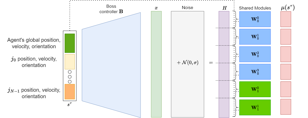
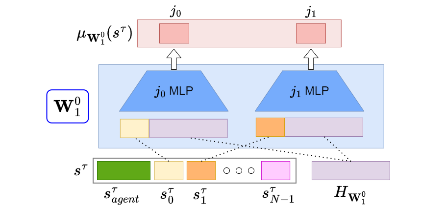
As shown in Fig. 10, the modular architecture starts by executing the boss controller B, which takes the full observation vector as input. The full observation vector includes both global observations about the agent and local observations of each actuator. The global observations consist of the agent’s global position, orientation, and velocity, while the local observations are composed of joint angle, joint velocity, and local relative position and orientation in the corresponding module’s frame. Given the full observation vector , outputs a latent vector of length , where is the size of the embedding sent to each module.
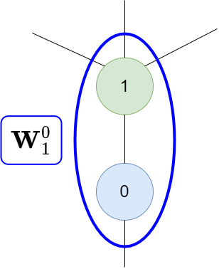
The latent vector is then split into segments of size and fed to modules. As shown in Fig. 11, a module itself consists of a MLP for each actuator . Each MLP takes as input ’s local features concatenated with the module’s segment of the latent vector and outputs the mean value of the action applied to .
A.4 Decomposition of Noise Injection Loss
A.5 Negative Log Likelihood Loss
In practice, we minimize the negative log likelihood loss during imitation learning. Similar to the above derivation, show that negative log likelihood with noise injection can be written in terms of the behavior cloning and invariance to noise losses. Let be our modular policy, where the mean of the Gaussian distribution for each of the actions is given by , and the standard deviation is a trainable vector, . We define the behavior cloning and invariance to noise losses as negative log likelihoods in Eq. 11 and 13 respectively.
| (10) | ||||
| (11) |
| (12) | ||||
| (13) |
We now consider the conditional log likelihood with noise injection and show how it can be decomposed in terms of the above losses.
| (14) | ||||
| (15) | ||||
| (16) | ||||
| (17) |
where is the product term.
A.6 Further Experimental Details
Let be the base hidden size of the network. As typical in PPO, we use Tanh nonlinearities and orthogonal initialization for the standard MLP and modular architectures. The standard MLP and boss controller are 2 layer neural networks. The size of the first layer is while the second layer has hidden units, where is the number of modules. The standard MLP also has a final linear layer to decode the actions. For all policy architecture variants, the value function is defined as a 2 layer neural network with hidden units each, followed by a linear layer.
In PPO, agents iteratively sample trajectories based on the current policy and subsequently perform optimization on a surrogate objective that first-order approximates the natural gradient. The surrogate objective prevents unstable updates to the policy by clipping the probability ratio . Optimizing the clipped objective is done with the policy gradient [23]. The RL loss that all architectures optimize includes the surrogate objective, a weighted value function loss, and a weighted entropy bonus to encourage exploration:
| (18) |
where is the generalized advantage estimation (GAE) [24]. is the clip value, is the weight on the value function, and is used to balance the entropy bonus.
We use Adam as the optimizer for both RL and IL. Semicolon-separated entries denote different values for the two domains: “[Locomotion Value]; [Grasping Value]". We conduct an extensive hyperparameter search and find that that the values in Table 2 yield reasonable performance.
| Parameters | Value Set |
|---|---|
| Value Loss Factor | 0.5 |
| Entropy Bonus Factor | 0 |
| Discount Factor | 0.995 |
| GAE | 0.95 |
| PPO Clip Value | 0.2 |
| Gradient Clip Value | 0.5 |
| Starting Learning Rate | 3e-4 |
| Number of Iterations per Update | 10 |
| Learning Rate Scheduler | Decay |
| Number of Processes | 8; 16 |
| Batch Size | 2048; 100 |
| Number of Timesteps | 8e6; 3e5 |
| Base Hidden Size | 128; 64 |
For experiments with pretrained policy weights, we initialize the learned logstd to -1.0. For all models on the locomotion tasks, we perform a secondary search over the batch size in [256, 512, 1024, 2048] until performance decays. We find that MeMo works best with smaller batch sizes: 256 on the 12 leg centipede, 512 on the 10 leg worm, and 1024 on the 10 leg hybrid. The modular architecture also sees an improvement when using 1024 for all three robots, whereas the default batch size of 2048 works best for the MLP architecture. NerveNet-Conv and NerveNet-Snowflake improve with a batch size of 1024 on the 12 leg centipede and 10 leg worm. We do not see a significant improvement when decreasing the batch size for MetaMorph. Due to the higher variance in reward for grasping tasks, we keep the same batch size for the transfer experiments.
For the modular architectures, we parameterize each joint network within the modules with a 2 layer MLP with 32 hidden units per layer. For imitation learning, we use a batch size of 1024 and tune the learning rate in [7e-4, 1e-3, 2e-3, 4e-3, 7e-3]. All models are trained for 175 iterations of DAgger. We sample 500 trajectories from the expert controllers of the 6 leg centipede, 6 leg worm, and 6 leg hybrid and 250 trajectories from the controller of the 4 finger claw as the validation sets. We make sure that the architectures pretrained with imitation learning achieve a comparable average reward as the expert controller when a number of trajectories are sampled from them.
For NerveNet, the input network is a single layer with size followed by a Tanh nonlinearity. We have a separate output network for each joint, and each output network is a 2 layer MLP with 32 units per layer. Table 3 summarizes the hyperparameter search that we perform for NerveNet. We perform grid search over the number of layers and the size of the messages passed by the propagation network. We choose the smallest architecture size that achieves a similar average reward as MeMo. Adding a skip connection from the root to all joints improves NerveNet’s validation score in imitation learning and enables the use of smaller architectures that do not overfit as easily.
| Parameters | Value Tried |
|---|---|
| Number of Layers | 2, 3, 4 |
| Message Size | 32, 64, 128 |
| Skip Connection | Yes, No |
For MetaMorph, we tune the number of attention layers in [2, 3, 4] and otherwise use the same architecture hyperparameters as [3], listed in Table 4. For a fair comparison, we use a MLP critic with the Transformer policy during RL rather than a Transformer critic, as the critic is trained from scratch during transfer. We find that positional encoding improves imitation learning pretraining, enabling the use of smaller architectures. For each token that corresponds to a joint, we include the one-hot encoding of the joint type in the observations.
| Parameters | Value |
|---|---|
| Number of Attention Heads | 1 |
| Embedding Dimension | 128 |
| Feedforward Dimension | 1024 |
| Nonlinearity | ReLU |
| Dropout | 0.1 |
A.7 State Space Description
We keep a running mean and variance to normalize the state space. Relative positions / orientations are relative to a joint in the same module as a given joint. For grasping, we use relative joint orientations as global joint orientations depend significantly on how high the claw is lifted. Table 5 and 6 detail the observation space in locomotion and grasping. For locomotion, “base" refers to the forwardmost wide body segment of the robot. As the joints are hinge joints, they only have one degree of freedom. The token type refers to the observation processing for MetaMorph – each input sequence consists of a single “global" token with the corresponding global observations for the robot concatenated with zero padding for the local observations, and the rest of the tokens are “joint" tokens with zero padding for the global observations concatenated with the local observations of the corresponding joint. We choose to integrate global information at the encoder level rather than the decoder level as our global features are low-dimensional: only 16 dimensions at most. The original MetaMorph architecture considers exteroceptive features from camera or depth sensors as global, which are much higher dimensional and are concatenated at the decoder level to prevent the dilution of local proprioceptive information.
| Controller Type | Node Type | Token Type | Observation Type | Axis |
| base position | y | |||
| base velocity | x | |||
| base velocity | y | |||
| base velocity | z | |||
| boss | root | global | base angular velocity | x |
| base angular velocity | y | |||
| base angular velocity | z | |||
| base orientation | x | |||
| base orientation | y | |||
| base orientation | z | |||
| joint position | - | |||
| joint velocity | - | |||
| joint orientation | x | |||
| boss, module | joint | joint | joint orientation | y |
| joint orientation | z | |||
| joint relative position | x | |||
| joint relative position | y | |||
| joint relative position | z |
| Controller Type | Node Type | Token Type | Observation Type | Axis |
| relative fingertip position to object | x | |||
| boss | root | global | relative fingertip position to object | y |
| relative fingertip position to object | z | |||
| joint position | - | |||
| joint velocity | - | |||
| joint relative orientation | x | |||
| boss, module | joint | joint | joint relative orientation | y |
| joint relative orientation | z | |||
| joint relative position | x | |||
| joint relative position | y | |||
| joint relative position | z |
A.8 Computing Infrastructure
We run experiments on 2 different machines with AMD Ryzen Threadripper PRO 3995WX processors and NVIDIA RTX A6000 GPUs. Both machines have 64 CPU cores and 128 threads. The main cost of running the agent in both the RoboGrammar and the DiffRedMax environments is the cost of simulation, which is CPU-intensive. For the MLP-based architectures, we only use CPU cores for computing rollouts in parallel environments via vectorization and backpropagating the policy gradient. For NerveNet, in the locomotion domain, we find it helpful to vectorize environments while performing backpropagation with a GPU. For example, the RL stage of MeMo on the 6 leg centipede takes less than a day to complete, whereas training a 3 layer NerveNet-Conv with the same number of processes and batch size requires 3-4 days without a GPU. We note that our resources are shared, and the wallclock time varies depending on the other processes running on the same server.
A.9 Additional environment details
We provide more details on the RoboGrammar tasks. On all locomotion tasks, the maximum episode length is 128. Full details of the environments can be found in the RoboGrammar codebase [16].
-
•
Frozen Terrain: A flat surface with a friction coefficient of 0.05.
-
•
Ridged Terrain: Ridges are placed an average of one meter apart across the width of the terrain.
-
•
Gap Terrain: A series of platforms separated by gaps.
-
•
Stepped Terrain: A series of steps with varying height, resembling a flight of stairs.
For all RoboGrammar locomotion environments, the reward at timestep is the sum of the rewards at each sub-step . The training reward function at substep is
| (19) |
where is the dimension of the action vector, and each dimension is normalized to [-1, 1]. The first two terms encourage high velocity in the -direction and maintaining the robot’s initial orientation respectively. The last term is a regularization penalty to reduce the variance across different runs. The reported reward curves do not include the regularization penalty.
For grasping, the goal is to grasp an object and lift it as high as possible and the maximum episode length is 50. As in prior work [6], we follow the convention of controlling the actuators with relative positions rather than absolute positions. The reward at timestep is the sum of the rewards at each sub-step . The full set of parameters used to construct the DiffRedMax simulation will be released with our source code. Below is the reward function used, where refers to the object’s z-coordinate and avg_fingertip_dist is the mean distance of the claw’s fingertips to the object’s surface. We approximate the cube’s surface with the surface of the largest sphere that fits in the cube. all_fingers_in_contact checks whether or not all fingers of the claw is within a small distance from the surface of the object.
The penalty on avg_fingertip_dist encourages the fingers to grasp the object. We only include the reward term on when all_fingers_in_contact is satisfied in order to prevent the claw from throwing the object.
A.10 Sources
We use the PPO implementation provided in https://github.com/ikostrikov/pytorch-a2c-ppo-acktr-gail (MIT License). Our NerveNet implementation is adapted from a PyTorch version of the original NerveNet codebase: https://github.com/HannesStark/gnn-reinforcement-learning. We adapt our MetaMorph implementation from the official codebase: https://github.com/agrimgupta92/metamorph/tree/main. We use the official RoboGrammar [16] (MIT License) and DiffRedMax [17] (MIT License) simulators.
A.11 Extended Related Works
Noise Injection. One line of work focuses on explaining the generalization benefits induced by noise injection by deriving explicit regularization terms. [25] studies Gaussian noise injected into network activations at each layer and derive an explicit regularization term by marginalizing out the noise. [26] analyzes the effect of Gaussian noise injection to the training data and find that the effect is equal to weighted ridge regularization as the number of noise injections approaches infinity. [27] study injecting noise into RNN hidden states and identify an explicit regularizer for small noise variances.
Hierarchical and Multi-Task RL. Our proposed modular architecture bears similarity to those used in hierarchical RL [28, 14]. However, a key difference is that our architecture is hierarchical with respect to the morphology of the robot, not the temporal structure of the task. To train robots that perform a diverse set of skills and generalize to new tasks, prior work leverages the shared structure of tasks, such as through graph representations [29, 30] that represent task compositionality, or through language representations [31, 32]. While many works in MTRL focus on a single morphology, recent efforts [33] have proposed representing both morphology and task in a single graph, enabling architectures trained on this unified IO representation to transfer to unseen morphologies and tasks.
Multi-Robot Coordination. Past works in multi-robot coordination bear similarity to our work in either the modularity of the architecture or the learning of a higher-level coordination mechanism, analogous to our boss controller, between different agents. In particular [34] uses a modular architecture, in which a higher-level meta-policy coordinates various skills with a behavior embedding. [35] proposes to learn a useful latent action space for coordinating a multiagent system via an information bottleneck. The information bottleneck helps in learning a latent action space from the full set of observations that is useful in coordinating decentralized agents at inference time.
A.12 Additional Experiments
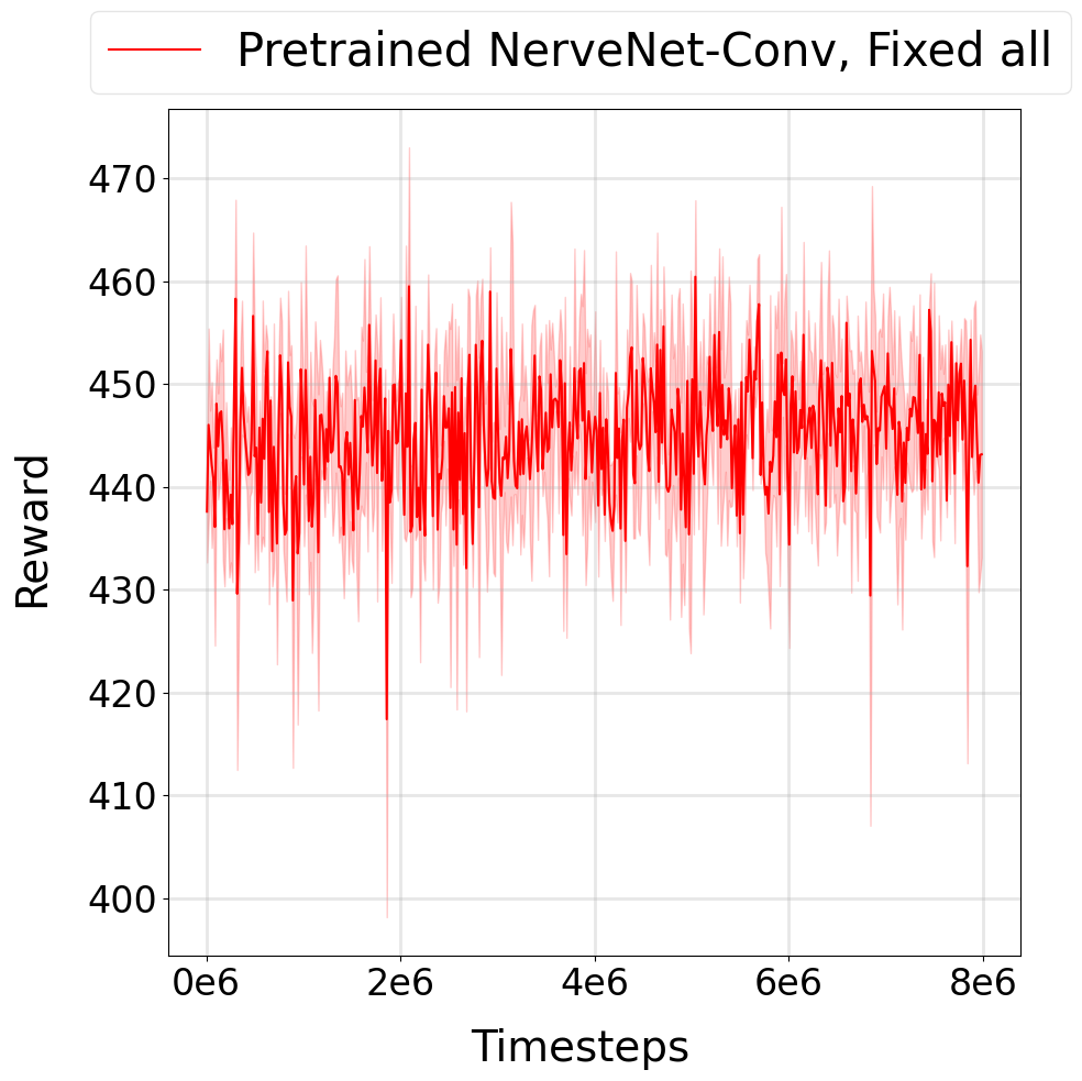
In Fig. 12, we test the zero-shot generalization of the pretrained NerveNet-Conv baseline by fixing all of its weights and only training the learned standard deviation when transferring from the 6 to the 12 leg centipede. Its poor performance demonstrates the difficulty of the transfer task, in spite of the physical similarities between the 6 and the 12 leg centipede.
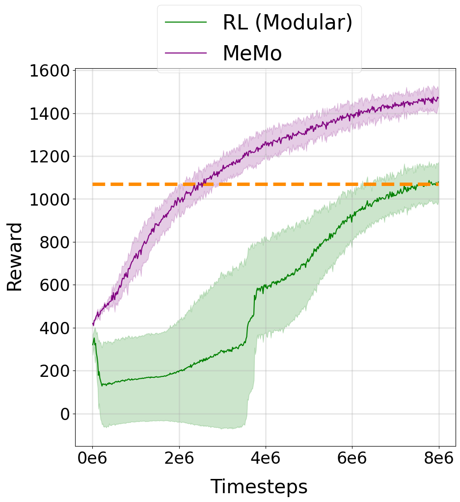
In addition, we demonstrate the capability of MeMo is scaling to much higher dimensionalities by transferring from a 6 to a 24 leg centipede (Fig. 13) on Frozen Terrain. MeMo significantly outperforms RL (Modular), the strongest baseline on the 6 to 12 leg centipede transfer task.
In Fig. 14, we test the transfer capabilities of MeMo to morphologies smaller than the starting structure. Specifically, we transfer modules from a 6 leg to a 4 leg centipede on the Frozen Terrain and from a 4 finger to a 3 finger claw grasping a cube. MeMo achieves improved training efficiency to policies trained from scratch and performs similarly to the strongest baseline in each domain.

In Fig. 15, we compare the singular value distributions of MeMo to the ablations described in Section 5.3 and MeMo with a lower value of . In Fig. 16, we run MeMo on the 6 to 12 leg centipede transfer where either the boss controller or the modules are 4 layer MLPs instead of 2. Both of these variants perform similarly to the original architecture.
A.13 Additional Figures
