Revisiting Random Walks for Learning on Graphs

Abstract

We revisit a simple idea for machine learning on graphs, where a random walk on a graph produces a machine-readable record, and this record is processed by a deep neural network to directly make vertex-level or graph-level predictions. We refer to these stochastic machines as random walk neural networks, and show that we can design them to be isomorphism invariant while capable of universal approximation of graph functions in probability. A useful finding is that almost any kind of record of random walk guarantees probabilistic invariance as long as the vertices are anonymized. This enables us to record random walks in plain text and adopt a language model to read these text records to solve graph tasks. We further establish a parallelism to message passing neural networks using tools from Markov chain theory, and show that over-smoothing in message passing is alleviated by construction in random walk neural networks, while over-squashing manifests as probabilistic under-reaching. We show that random walk neural networks based on pre-trained language models can solve several hard problems on graphs, such as separating strongly regular graphs where the 3-WL test fails, counting substructures, and transductive classification on arXiv citation network without training. Code is available at https://github.com/jw9730/random-walk.

1 Introduction

The most widely used class of neural networks on graphs are message passing neural networks where each vertex keeps a feature vector and updates it by propagating and aggregating messages over neighbors [67, 51, 46]. These networks benefit in efficiency by respecting the natural symmetries of graph functions, namely invariance to graph isomorphism [21]. On the other hand, message passing can be viewed as implementing color refinement iterations of the one-dimensional Weisfeiler-Lehman (1-WL) graph isomorphism test, and consequently their expressive power is not stronger [112, 83]. Also, the inner working of these networks is tied to the topology of the input graph, which is related to over-smoothing, over-squashing, and under-reaching of features under mixing [106, 48, 85].

In this work, we (re)visit a simple alternative idea for learning on graphs, where a random walk on a graph produces a machine-readable record, and this record is processed by a deep neural network that directly makes vertex-level or graph-level predictions. We call these stochastic machines random walk neural networks. Using random walks for graph learning has received practical interest due to their scalability and compatibility with sequence learning methods. This has led to empirically successful algorithms such as DeepWalk [94] and node2vec [50] which use skip-gram models on random walks and CRaWl [105] which uses convolutions on random walks. However, principled understanding and design of random walk neural networks have been studied relatively less.

We study the fundamental properties of random walk neural networks, and show that they can be designed from principle to be isomorphism invariant while capable of universal approximation of graph functions in probability. Specifically, we find that (1) almost any kind of record of random walks guarantees invariance as long as the vertices are anonymized, and there is no constraint on the choice of the neural network that processes the records, and (2) universal approximation is achieved if the neural network that reads the records is powerful enough, and the random walk covers the whole graph of interest with a high probability. The findings motivate us to record random walks in plain text and adopt a pre-trained transformer language model to read these records to solve graph tasks. They also give us principled guidance on how to design the random walk algorithm to minimize or bound the cover times, such as using restarts when working on a large and possibly infinite graph.

We further analyze random walk neural networks using tools from Markov chain theory and establish a parallelism to a simple model of message passing neural networks. From this, we show that over-smoothing phenomenon in message passing is inherently avoided in random walk neural networks, while over-squashing manifests as probabilistic under-reaching. This eliminates the typical trade-off between over-smoothing and over-squashing in message passing and allows our method to focus on overcoming under-reaching using rapidly mixing random walks such as non-backtracking walks.

We test random walk neural networks based on pre-trained language models on several hard problems on graphs. Our model based on DeBERTa [52] learns and performs separation of strongly regular graphs with perfect accuracy whereas the 3-WL test fails, and it also successfully learns challenging tasks of counting 8-cycles at graph-level and vertex-level. We further show that our approach can turn transductive classification problem on a large graph into an in-context learning problem by recording labeled vertices during random walks. To demonstrate this, we apply frozen Llama 3 [80] directly on transductive classification on arXiv citation network with 170k vertices, and show that it outperforms message passing networks as well as zero- and few-shot baselines even without training. This verifies that our approach allows a pure language model to understand and leverage graph structures.

2 Random Walk Neural Networks

Figure 1: A random walk neural network that reads text record using a language model.

We define a random walk neural network as a randomized function $X_{\theta}(\cdot)$ that takes a graph $G$ as input and outputs a random variable $X_{\theta}(G)$ on the output space $\mathbb{R}^{d}$. It can be optionally queried with an input vertex $v$ which gives a random variable $X_{\theta}(G,v)$. It consists of the following:

1. Random walk algorithm that produces $l$ steps of vertex transitions $v_{0}\to\cdots\to v_{l}$ on the input graph $G$. If an input vertex $v$ is given, we fix the starting vertex by $v_{0}=v$.

2. Recording function $q:(v_{0}\to\cdots\to v_{l},G)\mapsto\mathbf{z}$ that produces a machine-readable record $\mathbf{z}$ of the random walk. It may access the graph $G$ to record auxiliary information such as attributes.

3. Reader neural network $f_{\theta}:\mathbf{z}\mapsto\hat{\mathbf{y}}$ that processes record $\mathbf{z}$ and outputs a prediction $\hat{\mathbf{y}}$ in $\mathbb{R}^{d}$. It is the only trainable component and is not restricted to specific architectures.

To perform graph-level tasks, we sample a prediction $\hat{\mathbf{y}}\sim X_{\theta}(G)$ by running a random walk on $G$ and processing its record using the reader neural network. For vertex-level predictions $\hat{\mathbf{y}}\sim X_{\theta}(G,v)$, we query the input vertex $v$ by simply starting the random walk from it.

In the sections below, we discuss the design of each component for graph-level tasks on finite graphs and then vertex-level tasks on possibly infinite graphs. The latter simulates learning problems on large graphs, such as transductive classification, and forces the model to operate independently of the size of the whole graph $G$ [81]. Pseudocode and proofs can be found in Appendix A.2 and A.4.

2.1 Graph-Level Tasks

Let $\mathbb{G}$ be the class of undirected, connected, and simple graphs. Let $n\geq 1$ and $\mathbb{G}_{n}$ be the collection of graphs in $\mathbb{G}$ with at most $n$ vertices. We would like to model a graph-level function $\phi:\mathbb{G}_{n}\to\mathbb{R}^{d}$ using a random walk neural network $X_{\theta}(\cdot)$.

Since $\phi$ is a function on graphs, it is reasonable to assume that it is isomorphism invariant:

$$\phi(G)=\phi(H),\quad\forall G\simeq H.$$ (1)

Incorporating the invariance structure to our model class would offer generalization benefit [76, 13]. Since $X_{\theta}(\cdot)$ is a randomized function, we accept the probabilistic notion of invariance [63, 12, 26, 25]:

$$X_{\theta}(G)\overset{d}{=}X_{\theta}(H),\quad\forall G\simeq H.$$ (2)

We now claim that we can achieve probabilistic invariance by properly choosing the random walk algorithm and recording function while not imposing any constraint on the reader neural network.

Theorem 2.1.

$X_{\theta}(\cdot)$ is invariant if its random walk algorithm and recording function are invariant.

Below, we describe the choice of random walk algorithm, recording function, and neural networks that comprise random walk neural networks as in Theorem 2.1. Pseudocode is given in Appendix A.2.

Random walk algorithm

A random walk algorithm is invariant if it satisfies the following:

$$\pi(v_{0})\to\cdots\to\pi(v_{l})\overset{d}{=}u_{0}\to\cdots\to u_{l},\quad\forall G\overset{\pi}{\simeq}H,$$ (3)

where $v_{[\cdot]}$ is a random walk on $G$, $u_{[\cdot]}$ is a random walk on $H$, and $\pi:V(G)\to V(H)$ specifies the isomorphism from $G$ to $H$. It turns out that many random walk algorithms in literature are already invariant. To see this, let us write the probability of walking from a vertex $u$ to its neighbor $x\in N(u)$:

$$\mathrm{Prob}[v_{t}=x|v_{t-1}=u]\coloneq\frac{c_{G}(u,x)}{\sum_{y\in N(u)}c_{G}(u,y)},$$ (4)

where the function $c_{G}:E(G)\to\mathbb{R}_{+}$ assigns positive weights called conductance to edges. If we use constant conductance $c_{G}(\cdot)=1$, we have unbiased random walk used in DeepWalk [94]. We show:

Theorem 2.2.

The random walk in Equation (4) is invariant if its conductance $c_{[\cdot]}(\cdot)$ is invariant:

$$c_{G}(u,v)=c_{H}(\pi(u),\pi(v)),\quad\forall G\overset{\pi}{\simeq}H.$$ (5)

It includes constant conductance, and any choice that only uses degrees of endpoints $\mathrm{deg}(u)$, $\mathrm{deg}(v)$.

We favor using the degree information since it is cheap while potentially improving the behaviors of walks. Among many instantiations, we find that the following conductance function called the minimum degree local rule [3, 29] is particularly useful:

$$c_{G}(u,v)\coloneq\frac{1}{\min[\mathrm{deg}(u),\mathrm{deg}(v)]}.$$ (6)

This conductance is special because it achieves $O(n^{2})$ cover time, i.e. the expected time of visiting all $n$ vertices of a graph, optimal among random walks in Equation (4) that use degrees of endpoints [29].

In practice, we find that adding non-backtracking property that enforces $v_{t+1}\neq v_{t-1}$ is helpful while not adding much cost. Formally, we can extend Equation (4) and Theorem 2.2 to second-order random walks that include non-backtracking and node2vec walks [50]. We leave this in Appendix A.1.

Recording function

A recording function $q:(v_{0}\to\cdots\to v_{l},G)\mapsto\mathbf{z}$ takes a random walk and produces a machine-readable record $\mathbf{z}$. We let $q(\cdot,G)$ have access to the graph $G$ the walk is taking place. This allows recording auxiliary information such as vertex or edge attributes. A recording function is invariant if it satisfies the following for any given random walk $v_{[\cdot]}$ on $G$:

$$q(v_{0}\to\cdots\to v_{l},G)=q(\pi(v_{0})\to\cdots\to\pi(v_{l}),H),\quad\forall G\overset{\pi}{\simeq}H.$$ (7)

Invariance requires that $q(\cdot,G)$ produces the same record $\mathbf{z}$ regardless of re-indexing of vertices of $G$ into $H$. For this, we have to be careful in how we represent each vertex in a walk $v_{0}\to\cdots\to v_{l}$ as a machine-readable value, and which auxiliary information we record from $G$. We make two choices:

• Anonymization. We name each vertex in a walk with a unique integer, starting from $v_{0}\mapsto 1$ and incrementing it based on their order of discovery. For instance, a random walk $a\to b\to c\to a$ translates to a sequence $1\to 2\to 3\to 1$.

• Anonymization + named neighborhoods. While applying anonymization for each vertex $v$ in a walk, we record its neighbors $u\in N(v)$ if they are already named but the edge $v\to u$ has not been recorded yet. For instance, a walk $a\to b\to c\to d$ on a fully-connected graph translates to a sequence $1\to 2\to 3\langle 1\rangle\to 4\langle 1,2\rangle$, where $\langle\cdot\rangle$ represents the named neighborhoods.

The pseudocode of both algorithms can be found in Appendix A.2. We now show the following:

Theorem 2.3.

A recording function $q:(v_{0}\to\cdots\to v_{l},G)\mapsto\mathbf{z}$ that uses anonymization, optionally with named neighborhoods, is invariant.

Our choice of anonymizing a walk is inspired by the observation model of Micali and Zhu (2015) [81]. While initially motivated by privacy concerns [81, 60], we find it useful for invariance. Recording named neighborhoods is inspired by sublinear algorithms that probe previously discovered neighbors during a walk [28, 23, 10]. In our context, it is useful because whenever a walk visits a set of vertices $S\subseteq V(G)$ it automatically records the entire induced subgraph $G[S]$. As a result, to record all edges of a graph, a walk only has to visit all vertices. It is then possible to choose a random walk algorithm that takes only $O(n^{2})$ time to visit all $n$ vertices [3, 29], while traversing all edges, i.e. edge cover time, is $O(n^{3})$ in general [122, 89]. The degree-biasing in Equation (6) precisely achieves this.

Reader neural network

A reader neural network $f_{\theta}:\mathbf{z}\mapsto\hat{\mathbf{y}}$ processes the record $\mathbf{z}$ of the random walk and outputs a prediction $\hat{\mathbf{y}}$ in $\mathbb{R}^{d}$. As in Theorem 2.1, there is no invariance constraint imposed on $f_{\theta}$, and any neural network that accepts the recorded walks and has a sufficient expressive power can be used. This is in contrast to message passing where invariance is hard-coded in feature mixing operations. Furthermore, our record $\mathbf{z}$ can take any format, such as a matrix, byte sequence, or plain text, as long as $f_{\theta}$ accepts it. It is appealing in this regard to choose the record to be plain text, such as "1-2-3-1", and choose $f_{\theta}$ to be a pre-trained transformer language model. This offers expressive power [114] as well as transferable representation from language domain [75, 97]. In our experiments, we test both "encoder-only" DeBERTa [52] and "decoder-only" Llama [107] language models as $f_{\theta}$.

2.2 Vertex-Level Tasks

We now consider vertex-level tasks. In case of finite graphs, we may simply frame a vertex-level task $(G,v)\mapsto\mathbf{y}$ as a graph-level task $G^{\prime}\mapsto\mathbf{y}$ where $G^{\prime}$ is $G$ with its vertex $v$ marked. Then, we can solve $G^{\prime}\mapsto\mathbf{y}$ by querying a random walk neural network $X_{\theta}(G,v)$ to start its walk at $v_{0}=v$.

A more interesting case is when $G$ is an infinite graph that is only locally finite, i.e., has finite degrees. This simulates learning problems on a large graph such as transductive classification. In this case, it is reasonable to assume that our target function depends on finite local structures [103, 81].

Let $r\geq 1$, and $\mathbb{B}_{r}\coloneq\{B_{r}(v)\}$ be the collection of local balls in $G$ of radius $r$ centered at $v\in V(G)$. We would like to model a vertex-level function $\phi:\mathbb{B}_{r}\to\mathbb{R}^{d}$ on $G$ using a random walk neural network $X_{\theta}(\cdot)$ by querying the vertex of interest, $X_{\theta}(G,v)$. We assume $\phi$ is isomorphism invariant:

$$\phi(B_{r}(v))=\phi(B_{r}(u)),\quad\forall B_{r}(v)\simeq B_{r}(u).$$ (8)

The invariance of $X_{\theta}(\cdot)$ in probability is defined as following:

$$X_{\theta}(G,v)\overset{d}{=}X_{\theta}(G,u),\quad\forall B_{r}(v)\simeq B_{r}(u).$$ (9)

We may achieve invariance by choosing the random walk algorithm and recording function similar to the graph-level case. As a modification, we query $X_{\theta}(G,v)$ with the starting vertex $v_{0}=v$ of the random walk. Anonymization informs $v$ to the reader neural network by always naming it as $1$.

Then, we make an important choice of localizing random walks with restarts. That is, we reset a walk to the starting vertex $v_{0}$ either with a probability $\alpha\in(0,1)$ at each step or periodically every $k$ steps. A restarting random walk tends to stay more around its starting vertex $v_{0}$, and was used to implement locality bias in personalized PageRank algorithm for search [88, 44]. This localizing effect is crucial in our context since a walk may drift away from $B_{r}(v_{0})$ before recording all necessary information, which will then take an infinite time to return since $G$ is infinite [35, 61, 16, 79]. Restarts make the return to $v_{0}$ mandatory, ensuring that $B_{r}(v_{0})$ can be recorded within a finite expected time. We show:

Theorem 2.4.

For a uniform random walk on an infinite graph $G$ starting at $v$, the cover time and edge cover time of the finite local ball $B_{r}(v)$ are not always finitely bounded.

Theorem 2.5.

In Theorem 2.4, if the random walk restarts at $v$ with any nonzero probability $\alpha$ or any period $k\geq r+1$, the cover time and edge cover time of $B_{r}(v)$ are always finite.

3 Analysis

In Section 2, we have described the design of random walk neural networks, primarily relying on the principle of invariance. In this section we provide in-depth analysis on their expressive power and relations to issues in message passing such as over-smoothing, over-squashing, and under-reaching.

3.1 Expressive Power

Intuitively, if the records of random walks contain enough information such that the structures of interest, e.g. graph $G$ or local ball $B_{r}(v)$, can be fully recovered, a powerful reader neural network such as a multi-layer perceptron [27, 55] or a transformer [114] on these records would be able to approximate any function of interest. Our following analysis shows this.

We first consider using random walk neural network $X_{\theta}(\cdot)$ to universally approximate graph-level functions $\phi(\cdot)$ in probability, as defined in Abboud et al. (2021) [1]. While we consider scalar-valued functions as often done in universality proofs, extension to vector-valued functions can be done easily.

Definition 3.1.

$X_{\theta}(\cdot)$ is a universal approximator of graph-level functions in probability if, for all invariant functions $\phi:\mathbb{G}_{n}\to\mathbb{R}$ for a given $n\geq 1$, and $\forall\epsilon,\delta>0$, there exist choices of length $l$ of the random walk and network parameters $\theta$ such that the following holds:

$$\mathrm{Prob}[|\phi(G)-X_{\theta}(G)|<\epsilon]>1-\delta,\quad\forall G\in\mathbb{G}_{n}.$$ (10)

We show that, if the random walk is long enough and the reader neural network $f_{\theta}$ is powerful enough, a random walk neural network $X_{\theta}(\cdot)$ is capable of graph-level universal approximation in probability. In particular, we show that the length of the random walk $l$ controls the confidence $1-\delta$ of the approximation, with cover time $C_{V}(G)$ or edge cover time $C_{E}(G)$ playing a central role.

Theorem 3.2.

A random walk neural network $X_{\theta}(\cdot)$ with a sufficiently powerful $f_{\theta}$ is a universal approximator of graph-level functions in probability (Definition 3.1) if it satisfies either of the below:

• It uses anonymization to record random walks of lengths $l>C_{E}(G)/\delta$.

• It uses anonymization and named neighborhoods to record walks of lengths $l>C_{V}(G)/\delta$.

We remark that, while the cover time and edge cover time are $O(n^{3})$ for uniform random walks [4, 122, 24, 41, 15, 2, 89, 45], we make use of minimum degree local rule in Equation (6) to achieve a cover time of $O(n^{2})$ [3, 29], in conjunction with named neighborhood recording. While universal approximation can be in principle achieved with simple uniform random walk, our design reduces the length $l$ required for the desired reliability $>1-\delta$, and hence improves learning and inference.

We now show an analogous result for universal approximation of vertex-level functions. Since our target function $\phi$ is on a collection $\mathbb{B}_{r}$ of finite graphs, the proof is similar to the graph-level case.

Definition 3.3.

$X_{\theta}(\cdot)$ is a universal approximator of vertex-level functions in probability if, for all invariant functions $\phi:\mathbb{B}_{r}\to\mathbb{R}$ for a given $r\geq 1$, and $\forall\epsilon,\delta>0$, there exist choices of length $l$ and restart probability $\alpha$ or period $k$ of the random walk and network parameters $\theta$ such that:

$$\mathrm{Prob}[|\phi(B_{r}(v))-X_{\theta}(G,v)|<\epsilon]>1-\delta,\quad\forall B_{r}(v)\in\mathbb{B}_{r}.$$ (11)

We show the following, which relates to local cover time $C_{V}(B_{r}(v))$ and edge cover time $C_{E}(B_{r}(v))$:

Theorem 3.4.

A random walk neural network $X_{\theta}(\cdot)$ with a sufficiently powerful $f_{\theta}$ and any nonzero restart probability $\alpha$ or restart period $k\geq r+1$ is a universal approximator of vertex-level functions in probability (Definition 3.3) if it satisfies either of the below for all $B_{r}(v)\in\mathbb{B}_{r}$:

• It uses anonymization to record random walks of lengths $l>C_{E}(B_{r}(v))/\delta$.

• It uses anonymization and named neighborhoods to record walks of lengths $l>C_{V}(B_{r}(v))/\delta$.

We remark that restarts are necessary to finitely bound the local cover times of a random walk on an infinite graph. From this fact and Theorem 3.4 we can see that non-restarting walks of finite length cannot provide vertex-level universal approximation in probability, and our design is obligatory.

3.2 Over-smoothing, Over-squashing, and Under-reaching

In message passing neural networks, the model operates by passing features over edges and mixing them, and thus their operation is tied to the topology of the input graph. It is now understood how this relates to the issues of over-smoothing, over-squashing, and under-reaching [9, 106, 47, 48, 85, 111]. We connect these theories and random walk neural networks to verify if similar issues may take place.

Let $G$ be a connected non-bipartite graph with row-normalized adjacency matrix $P$. We consider a simplified message passing model, where the vertex features $\mathbf{h}^{(0)}$ are initialized as some probability vector $\mathbf{x}$, and updated by $\mathbf{h}^{(t+1)}=\mathbf{h}^{(t)}P$. This simple model is often used as a proxy to study the aforementioned issues [48, 118]. For example, over-smoothing happens as the features exponentially converge to a stationary vector $\mathbf{h}^{(l)}\to\boldsymbol{\pi}$ as $l\to\infty$, smoothing out the input $\mathbf{x}$ [48]. Over-squashing and under-reaching occur when a feature $\mathbf{h}_{u}^{(l)}$ becomes insensitive to distant input $\mathbf{x}_{v}$. While under-reaching refers to insufficient depth $l<\mathrm{diam}(G)$ [9, 106], over-squashing refers to features getting overly compressed at bottlenecks of $G$, even with sufficient depth $l$. The latter is described by the Jacobian $|\partial\mathbf{h}_{u}^{(l)}/\partial\mathbf{x}_{v}|\leq[\sum_{t=0}^{l}P^{t}]_{uv}$,, as the bound often decays exponentially with $l$ [106, 11].

What do these results tell us about random walk neural networks? We can see that, while $P$ drives feature mixing in the message passing schema, it can be also interpreted as the transition probability matrix of uniform random walk where $P_{uv}$ is the probability of walking from $u$ to $v$. This parallelism motivates us to design an analogous, simplified random walk neural network and study its behavior.

We consider a simple random walk neural network that runs a uniform random walk $v_{0}\to\cdots\to v_{l}$, reads the record $\mathbf{x}_{v_{0}}\to\cdots\to\mathbf{x}_{v_{l}}$ by averaging, and outputs it as $\mathbf{h}^{(l)}$. Like simple message passing, the model involves $l$ steps of time evolution through $P$. However, while message passing uses $P$ to process features, this model uses $P$ only to obtain a record of input, with feature processing decoupled. We show that in this model, over-smoothing does not occur as in simple message passing:

Theorem 3.5.

The simple random walk neural network outputs $\mathbf{h}^{(l)}\to\mathbf{x}^{\top}\boldsymbol{\pi}$ as $l\to\infty$.

Even if the time evolution through $P$ happens fast (i.e. $P$ is rapidly mixing) or with many steps $l$, the model is resistant to over-smoothing as the input $\mathbf{x}$ always affects the output. In fact, if $P$ is rapidly mixing, we may expect improved behaviors based on Section 3.1 as the cover times could reduce.

On the other hand, we show that over-squashing manifests as probabilistic under-reaching:

Theorem 3.6.

Let $\mathbf{h}_{u}^{(l)}$ be output of the simple random walk neural network queried with $u$. Then:

$$\mathbb{E}\left[\left|\frac{\partial\mathbf{h}_{u}^{(l)}}{\partial\mathbf{x}_{v}}\right|\right]=\frac{1}{l+1}\left[\sum_{t=0}^{l}P^{t}\right]_{uv}\to\boldsymbol{\pi}_{v}\quad\text{as}\quad l\to\infty.$$ (12)

The equation shows that the feature Jacobians are bounded by the sum of powers of $P$, same as in simple message passing. Both models are subject to over-squashing phenomenon that is similarly formalized, but manifests through different mechanisms. While in message passing the term is related to over-compression of features at bottlenecks [106], in random walk neural networks it is related to exponentially decaying probability of reaching a distant vertex $v$, i.e., probabilistic under-reaching.

In message passing, it is understood that the topology of the input graph inevitably induces a trade-off between over-smoothing and over-squashing [85, 48]. Our results suggest that random walk neural networks avoid the trade-off, and we can focus on overcoming under-reaching e.g. by accelerating the walk, while not worrying much about over-smoothing. Our design choices such as degree-biasing (Equation (6)) and non-backtracking [5] can be understood as achieving this.

4 Related Work

Random walks on graphs

Our work builds upon theory of random walks on graphs, i.e. Markov chains on discrete spaces. Their statistical properties such as hitting and mixing times have been well-studied [4, 74, 24, 41, 86, 93], and our method (Section 2) is related to cover time [4, 62, 33, 2], edge cover time [122, 15, 89, 45], and improving them, using local degree information [59, 3, 29], non-backtracking [5, 64, 7, 39], or restarts in case of infinite graphs [35, 79, 61]. Random walks and their statistical properties are closely related to structural properties of graphs, such as effective resistance [34, 17], Laplacian eigen-spectrum [74, 102], and discrete Ricci curvatures [87, 32]. This has motivated our analysis in Section 3.2, where we transfer the prior results on over-smoothing and over-squashing of message passing based on these properties [9, 106, 47, 48, 11, 85, 91] into the results on our approach. Our work is also inspired by graph algorithms based on random walks, such as anonymous observation [81], sublinear algorithms [28, 23, 10], and personalized PageRank for search [88]. While we adopt their techniques to make our walks and their records well-behaved, the difference is that we use a deep neural network to process the records and directly make predictions.

Random walks and graph learning

In graph learning, random walks have received interest due to their scalability and compatibility to sequence learning methods. DeepWalk [94] and node2vec [50] use shallow skip-gram models on random walks to learn vertex embeddings. While CRaWl [105] is the most relevant to our work, it uses convolutions on walks recorded in a different way from ours. Hence, its expressive power is controlled by the kernel size and does not always support universality. AgentNet [78] learns agents that walk on a graph while recurrently updating their features. While optimizing the walk strategy, this method may trade off efficiency as training requires recurrent roll-out of the entire network. Our method allows pairing simple and fast walkers with parallelizable networks such as transformers, which suffices for universality. WalkLM [104] proposed a fine-tuning method for language models on random walks on text-attributed graphs. While in a similar spirit, our result provides more principles as well as extending to purely topological graphs and training-free setups. Our method is also related to label propagation algorithms [120, 121, 49] that perform transductive learning on graphs based on random walks, which we further discuss in Section 5.3.

Probabilistic invariant neural networks

Whenever a learning problem is compatible with symmetry, incorporating the associated invariance structure to the hypothesis class often leads to generalization benefit [13, 36, 37]. This is also the case for probabilistic invariant neural networks [76, 12], which includes our approach. Probabilistic invariant networks have recently gained interest due to their potential of achieving higher expressive powers compared to deterministic counterparts [26, 101]. In graph learning, this is often achieved with stochastic symmetry breaking between vertices using randomized features [73, 95, 1, 65], vertex orderings [84, 66], or dropout [90]. Our approach can be understood as using random walk as a symmetry-breaking mechanism for probabilistic invariance, which provides an additional benefit of natural compatibility with sequence learning methods.

Language models on graphs

While not based on random walks, there have been prior attempts on applying language models for problems on graphs [108, 20, 117, 40, 113], often focusing on prompting methods on problems involving simulations of graph algorithms. We take a more principle-oriented approach based on invariance and expressive power, and thus demonstrate our approach mainly on the related tasks, e.g. graph separation. We believe extending our work to simulating graph algorithms requires a careful treatment [109, 31, 30, 98] and plan to investigate it as future work.

5 Experiments

We perform a series of experiments to demonstrate random walk neural networks. We implement random walk algorithms in C++ based on Chenebaux (2020) [22], which produces good throughput even without GPU acceleration [105]. Likewise, we implement recording functions in C++ which perform anonymization with named neighborhoods and produce plain text. Pseudocode of our implementation is given in Appendix A.2. We choose reader neural networks as pre-trained language models, with a prioritization on long inputs in accordance to Section 3.1. For fine-tuning experiments, we use DeBERTa-base [52] that supports up to 12,276 tokens, and for training-free experiments, we use instruction-tuned Llama 3 [80] that support up to 8,192 tokens. We implement our pipelines in PyTorch [92] with libraries [42, 38, 110, 70] that support multi-GPU training and inference.

5.1 Graph Separation

Table 1: Graph separation results. We report accuracy of classifying training data rounded to the first decimal point. *, ${\dagger}$, ${\ddagger}$, $\mathsection$, and ^⋄ are from [90], [84], [119], [78], and [6], respectively. We trained AgentNet and CRaWl on SR25 with their reported best configurations on SR16 and CSL, respectively.

	CSL	SR16	SR25
Method	1, 2-WL fails	3-WL fails	3-WL fails
GIN [112]	10.0%${\dagger}$	50.0%$\mathsection$	6.7%${\ddagger}$
PPGN [77]	100.0%$\mathsection$	50.0%$\mathsection$	6.7%${\ddagger}$
GIN-AK+ [119]	-	-	6.7%${\ddagger}$
PPGN-AK+ [119]	-	-	100.0%${\ddagger}$
GIN+ELENE [6]	-	-	6.7%⋄
GIN+ELENE-L (ED) [6]	-	-	100.0%⋄
GIN-RNI [1, 100]	16.0%*	-	-
GIN-RP [84]	37.6%${\dagger}$	-	-
GIN-Dropout [90]	82.0%*	-	-
Random Walk AgentNet [78]	100.0%$\mathsection$	50.5%$\mathsection$	-
AgentNet [78]	100.0%$\mathsection$	100.0%$\mathsection$	6.7%
CRaWl [105]	100.0%$\mathsection$	100.0%$\mathsection$	46.6%
DeBERTa-walk (Ours)	100.0%	100.0%	100.0%

We first verify the claims on expressive power in Section 3.1 using three synthetic datasets where the task is recognizing the isomorphism type of an input graph. This is framed as fitting an $N$-way classification problem on $N$ non-isomorphic graphs. The graphs are chosen such that a certain WL graph isomorphism test fails, and so does their related family of message passing neural networks.

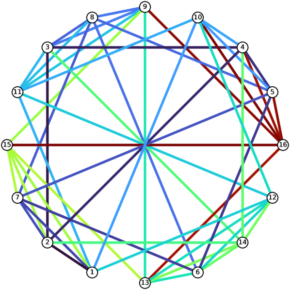
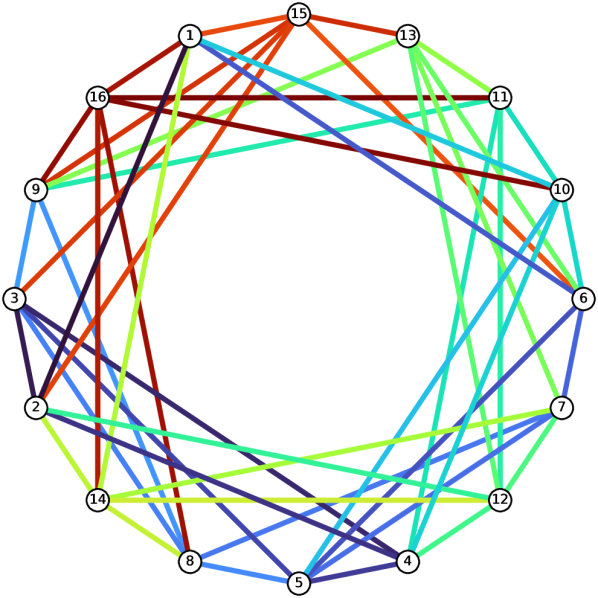
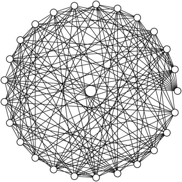
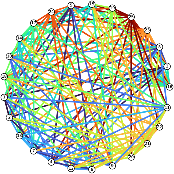
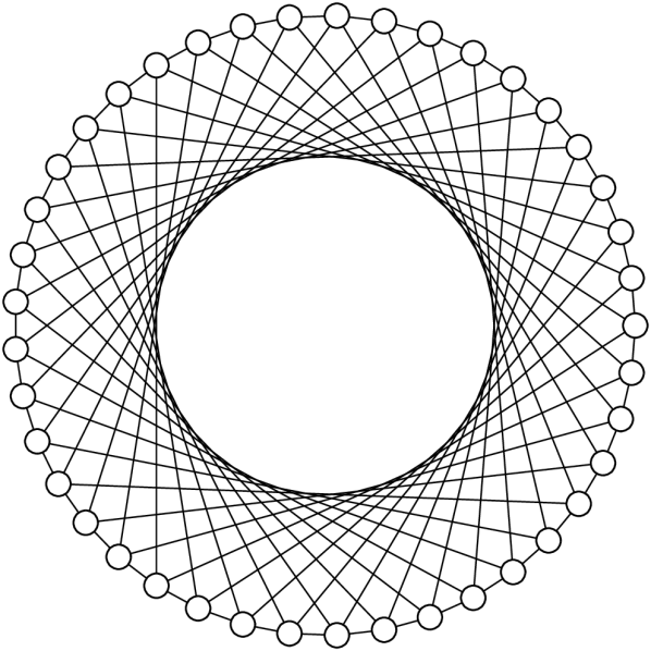
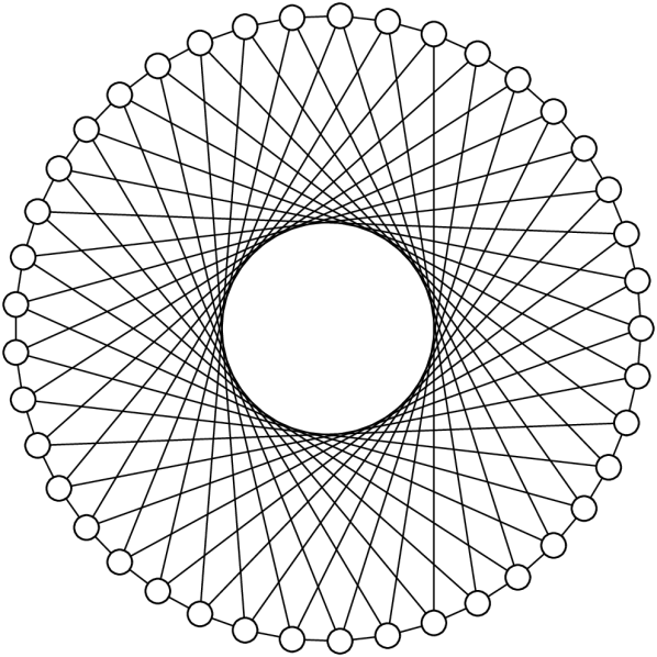
The Circular Skip Links (CSL) graphs dataset [84] contains 10 non-isomorphic regular graphs with 41 vertices of degree 4. Distinguishing these graphs requires computing lengths of skip links [78, 21], and 1-WL and 2-WL tests fail. The $4\times 4$ rook’s and Shrikhande graphs [6], which we call SR16, are a pair of strongly regular graphs with 16 vertices of degree 6. Distinguishing the pair requires detecting 4-cliques [78], and 3-WL test fails [6]. The SR25 dataset [8] contains 15 strongly regular graphs with 25 vertices of degree 12, on which 3-WL test fails [6]. SR25 is challenging and has only been solved by a handful of carefully designed subgraph-based message passing algorithms [82, 119, 6]. Examples of the considered graphs and random walks on them can be found in Appendix A.2.

Our random walk neural network uses the minimum degree local rule from Equation (6) with non-backtracking (Algorithm 1), and recording function with anonymization and named neighborhoods that produces plain text (Algorithm 3). We use pre-trained DeBERTa-base language model as the reader neural network, and fine-tune it with cross-entropy loss for at most 100k steps using AdamW optimizer [72] with 2e-5 learning rate and 0.01 weight decay on on 8$\times$ RTX 3090 GPUs. While the model supports 12,276 tokens in maximum, we use 512 tokens which is the maximum allowed by memory constraint. We use batch size 256, and accumulate gradients for 8 steps for SR25. At test time, we ensemble 4 stochastic predictions of the network by averaging classification logits.

The results are in Table LABEL:table:graph_separation. Message passing neural networks that align with certain WL test fail when asked to solve harder problems, e.g. GIN aligns with 1-WL and fails in CSL. Recent algorithms that use subgraphs and structural features show improved performance, with state-of-the-art such as ELENE-L (ED) solving SR25. Alternative approaches based on stochastic symmetry-breaking e.g. random node identification, often fail on CSL although universal approximation is possible in theory [1], possibly due to learning difficulties. For algorithms based on walks, AgentNet and CRaWl solve CSL and SR16, while failing on SR25. This is because learning a policy to walk in AgentNet can be challenging in complex tasks especially at the early stage of training, and the expressiveness of CRaWl is limited by the receptive field of convolution layers. Our approach based on DeBERTa language model overcomes the problems, being the first walk-based algorithm that solves SR25.

In Appendix A.3, we further provide visualizations of learned attentions by mapping attention weights on text records of walks to input graphs. We find that the models often focus on sparse, connected substructures, which presumably provide discriminative information on the isomorphism types.

5.2 Substructure Counting

Table 2: Substructure (8-cycle) counting results. We report normalized mean absolute error (MAE) on test set at best validation. We trained MP, Subgraph GNN, Local 2-GNN, and Local 2-FGNN using configurations in [115], and trained MP-RNI, MP-Dropout, AgentNet, and CRaWl as in Table LABEL:table:graph_separation.

Method	Graph-level	Vertex-level
MP [115]	.0917	.1156
Subgraph GNN [115]	.0515	.0715
Local 2-GNN [115]	.0433	.0478
Local 2-FGNN [115]	.0422	.0438
Local 2-FGNN (large)	.0932	.1121
MP-RNI [1, 100]	.3610	.3650
MP-Dropout [90]	.1359	.1393
AgentNet [78]	.1107	N/A
CRaWl [105]	.0526	.0725
DeBERTa-walk (Ours)	.0459	.0465

We test our model on more challenging tasks that require both expressive power and generalization to unseen graphs. We use a synthetic dataset of 5,000 random regular graphs from Chen et al. (2020) [19], and consider the task of counting substructures. We choose 8-cycles since they are known to require a particularly high expressive power [115]. We experiment with both graph-level and vertex-level counting i.e. counting 8-cycles containing the queried vertex, following Zhang et al. (2024) [115]. We use the data splits from the previous works [19, 119, 115], while excluding disconnected graphs following our modeling assumption in Section 2.1. Our random walk neural network uses the same design to Section 5.1, and we train them with L1 loss for at most 250k steps using batch size of 128 graphs for graph-level counting and 8 graphs for vertex-level. At test-time, we ensemble 64 and 32 stochastic predictions by averaging for graph- and vertex-level tasks, respectively.

The results are in Table LABEL:table:counting, and overall in line with Section 5.1. While simple message passing shows a low performance, variants with higher expressive powers such as local 2-GNN and local 2-FGNN achieve high performances. This is consistent with the observation of [115]. On the other hand, message passing with stochastic symmetry-breaking often show learning difficulties and does not achieve good performance. AgentNet was not directly applicable for vertex-level counting since its vertex encoding depends on which vertices the agent visits, and a learning difficulty was observed for graph-level counting. Our approach based on DeBERTa demonstrates competitive performance, outperforming random walk baselines and approaching performances of local 2-GNN and 2-FGNN.

5.3 In-Context Transductive Classification

Table 3: Transductive classification test accuracy on ogbn-arxiv. ${\dagger}$ denotes using validation labels for in-context learning or label propagation, as done in [58]. For Llama 3, we use instruction-tuned models, and ensemble 5 predictions by voting for both one-shot learning and our algorithm.

Method	Accuracy
MLP [57]	55.50%
node2vec [57]	70.07%
GCN [57]	71.74%
GAT [71]	73.91%
RevGAT [71]	74.26%
Label propagation [58]	68.50%
C&S [58]	72.62%
C&S${\dagger}$ [58]	74.02%
Llama2-13b zero-shot [53]	44.23%
GPT-3.5 zero-shot [53]	73.50%
DeBERTa, fine-tuned [116]	74.13%
Llama3-8b zero-shot	50.20%
Llama3-8b one-shot	52.49%
Llama3-8b one-shot${\dagger}$	52.54%
Llama3-8b-walk (Ours)	71.10%
Llama3-8b-walk (Ours)${\dagger}$	73.11%
Llama3-70b zero-shot	65.33%
Llama3-70b one-shot${\dagger}$	67.57%
Llama3-70b-walk (Ours)${\dagger}$	74.75%

Previous results considered synthetic tasks on undirected, unattributed, and relatively small graphs. We now show that our approach based on frozen Llama 3 [80] language models can solve real-world problem on a large graph with directed edges and textual attributes, without any training. We use ogbn-arxiv [57], a citation network of 169,343 arXiv papers with title and abstract attributes. The task is transductive classification into 40 areas such as "cs.AI" using a subset of labeled vertices.

We consider two representative types of baselines. The first reads title and abstract of each vertex using a language model and solves vertex-wise classification problem, ignoring graph structure. The second initializes vertex features as language model embeddings and trains a graph neural network, at the risk of over-compressing the text. Our algorithm allows taking the best of both worlds. We design the recording function so that, not only it does basic operations such as anonymization, it records a complete information of the local subgraph including title and abstract, edge directions, and notably, labels in case of labeled vertices (Appendix A.2) [99]. The resulting record naturally includes a number of input-label pairs of the classification task at hand, implying that we can frame transductive classification problem as a simple in-context learning problem [14]. This allows us to use a frozen Llama 3 [80] language model directly on transductive classification without any training.

The results are in Table LABEL:table:arxiv. Notably, our model based on frozen Llama 3 is able to outperform graph neural networks on text embeddings, as well as language models that perform vertex-wise predictions ignoring graph structures such as GPT-3.5 and fine-tuned DeBERTa. We especially note that our model largely outperforms one-shot baselines, which are given 40 randomly chosen labeled examples (one per class). This is surprising as our model observes fewer vertices, 29.17 in average, due to other recorded information. This is presumably since the record produced by our algorithm faithfully encodes graph structure, providing more useful input for the language model to quickly learn the task in-context compared to randomly chosen shots. Overall, the results show that our approach allows a pure language model to understand and leverage graph structures even without training. In Appendix A.3, we provide a visualization of the internal attention weights, verifying that the model makes use of the graph structure recorded by the random walk to make predictions.

As a final note, our approach is related to label propagation algorithms [120, 121, 49] for transductive classification, which makes predictions by running random walks and probing the distribution of visited labeled vertices. The difference is that, in our approach, the reader neural network i.e. language model can appropriately use other information such as attributes, as well as do meaningful non-linear processing rather than simply probing the input. As shown in Table LABEL:table:arxiv, our approach outperforms label propagation, verifying our intuition. This result also supports the proposal of Sato (2024) [99] of using labels as features for training-free neural networks for transductive classification on graphs.

6 Conclusion

We presented random walk neural networks, stochastic machines that process a graph as a machine-readable record of random walk. By choosing a proper random walk algorithm and recording function, the proposed method can achieve isomorphism invariance and universal approximation of graph functions in probability using unconstrained neural networks. Equipped with a powerful language model, the proposed method demonstrated promising results on a number of hard graph learning problems and even in-context learning capability on large-scale transductive classification tasks.

Limitations and future work

Our current main limitation is the cost of performing training and inference with language models, especially on long walks. We believe efficient fine-tuning with e.g. low-rank adaptation [56, 18] may help overcome the issue. A question for future work is whether we can train a language model on a large pseudocorpus of random walks [68, 69] to build a foundation model for graphs which is language-compatible. We plan to investigate this direction in the future.

Acknowledgements

This work was supported in part by the National Research Foundation of Korea (RS-2024-00351212) and the IITP grant (2022-0-00926 and RS-2022-II220959) funded by the Korean government (MSIT).

Appendix A Appendix

A.1 Second-Order Random Walks (Section 2.1)

In second-order random walks, the probability of choosing $v_{t+1}$ depends not only on $v_{t}$ but also on $v_{t-1}$. We consider non-backtracking [5, 43] and node2vec [50] random walks as representatives.

A non-backtracking random walk is defined upon a first-order random walk algorithm, e.g. one in Equation (4), by enforcing $v_{t+1}\neq v_{t-1}$:

$$\mathrm{Prob}[v_{t+1}=x|v_{t}=j,v_{t-1}=i]\coloneq\begin{dcases*}\frac{\mathrm{Prob}[v_{t+1}=x|v_{t}=j]}{\sum_{y\in N(j)\setminus\{i\}}\mathrm{Prob}[v_{t+1}=y|v_{t}=j]}&for $x\neq i$,\\ 0\vphantom{\frac{0}{0}}&for $x=i$,\end{dcases*}$$ (13)

where $\mathrm{Prob}[v_{t+1}=x|v_{t}=j]$ is the probability of walking $j\to x$ given by the underlying first-order random walk. Notice that the probabilities are renormalized over $N(j)\setminus\{i\}$. This is ill-defined in the case the walk traverses $i\to j$ and reaches a dangling vertex $j$ which has $i$ as its only neighbor, since $N(j)\setminus\{i\}=\emptyset$. In such cases, we allow the random walk to "begrudgingly" backtrack [96], $i\to j$ and then $j\to i$, given that it is the only possible choice due to the dangling of $j$.

In case of node2vec random walk [50], a weighting term $\alpha(v_{t-1},v_{t+1})$ with two (hyper)parameters, return $p$ and in-out $q$, is introduced to modify the behavior of a first-order random walk:

$$\mathrm{Prob}[v_{t+1}=x|v_{t}=j,v_{t-1}=i]\coloneq\frac{\alpha(i,x)\,\mathrm{Prob}[v_{t+1}=x|v_{t}=j]}{\sum_{y\in N(j)}\alpha(i,y)\,\mathrm{Prob}[v_{t+1}=y|v_{t}=j]},$$ (14)

where the probability $\mathrm{Prob}[v_{t+1}=x|v_{t}=j]$ is given by the underlying first-order random walk and $\alpha(v_{t-1},v_{t+1})$ is defined as follows using the shortest path distance $d(v_{t-1},v_{t+1})$:

$$\alpha(v_{t-1},v_{t+1})\coloneq\begin{dcases*}1/p&for $d(v_{t-1},v_{t+1})=0$,\\ 1&for $d(v_{t-1},v_{t+1})=1$,\\ 1/q&for $d(v_{t-1},v_{t+1})=2$.\\ \end{dcases*}$$ (15)

Choosing a large return parameter $p$ reduces backtracking since it decreases the probability of walking from $v_{t}$ to $v_{t-1}$. Choosing a small in-out parameter $q$ has a similar effect of avoiding $v_{t-1}$, with a slight difference that it avoids the neighbors of $v_{t-1}$ as well.

We now show an extension of Theorem 2.2 to the above second-order random walks:

Theorem A.1.

The non-backtracking random walk in Equation (13) and the node2vec random walk in Equation (14) are invariant if their underlying first-order random walk algorithm is invariant.

Proof.

The proof is given in Appendix A.4.3. ∎

A.2 Main Algorithm

We outline the main algorithms for the random walk and the recording function described in Section 2 and used in Section 5. Algorithm 1 shows the random walk algorithm, and Algorithms 2, 3, and 4 show the recording functions. For the random walk algorithm, we use non-backtracking described in Appendix A.1 and the minimum degree local rule conductance $c_{G}(\cdot)$ given in Equation (6) by default.

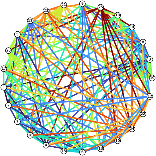
Based on the algorithms, in Figures 2, 3, and 4 we illustrate the task formats used for graph separation experiments in Section 5.1 by providing examples of input graphs, text records of random walks on them, and prediction targets for the language model that processes the records. Likewise, in Figures 5, 6, and 7 we show task formats for transductive classification on arXiv citation network in Section 5.3.

Data: Input graph $G$, optional input vertex $v$, conductance function $c_{G}:E(G)\to\mathbb{R}_{+}$, walk length $l$, optional restart probability $\alpha\in(0,1)$ or period $k>1$

Result: Random walk $v_{0}\to\cdots\to v_{l}$, restart flags $r_{1},...,r_{l}$

/* transition probabilities $p:E(G)\to\mathbb{R}_{+}$ */

1 for $(u,x)\in E(G)$ do

       $p(u,x)\leftarrow c_{G}(u,x)/\sum_{y\in N(u)}c_{G}(u,y)$

        // Equation (4)

2      

/* starting vertex $v_{0}$ */

3 if $v$ is given then

       /* query starting vertex */

4       $v_{0}\leftarrow v$

5      

6else

       /* sample starting vertex */

7       $v_{0}\sim\mathrm{Uniform}(V(G))$

8      

/* random walk $v_{1}\to\cdots\to v_{l}$, restart flags $r_{1},...,r_{l}$ */

9 $v_{1}\sim\mathrm{Categorical}(\{p(v_{0},x):x\in N(v_{0})\})$

10 $r_{1}\leftarrow 0$

11 for $t\leftarrow 2$ to $l$ do

       /* restart flag $r_{t}$ */

12       $r_{t}\leftarrow 0$

13       if $\alpha$ is given then

             /* if restarted at $t-1$, do not restart */

14             if $r_{t-1}=0$ then

15                   $r_{t}\sim\mathrm{Bernoulli}(\alpha)$

16                  

17            

18      else if $k$ is given then

19             if $t\equiv 0\pmod{k}$ then

20                   $r_{t}\leftarrow 1$

21                  

22            

      /* random walk $v_{t}$ */

23       if $r_{t}=0$ then

24             $S\leftarrow N(v_{t-1})\setminus\{v_{t-2}\}$

25             if $S\neq\emptyset$ then

                   /* non-backtracking */

                   $v_{t}\sim\mathrm{Categorical}(\{p(v_{t-1},x)/\sum_{y\in S}p(v_{t-1},y):x\in S\})$

                    // Equation (13)

26                  

27            else

                   /* begrudgingly backtracking */

28                   $v_{t}\leftarrow v_{t-2}$

29                  

30            

31      else

             /* restart */

32             $v_{t}\leftarrow v_{0}$

33            

34      

Algorithm 1 Random walk algorithm

Data: Random walk $v_{0}\to\cdots\to v_{l}$, restart flags $r_{1},...,r_{l}$

Result: Text record $\mathbf{z}$

/* named vertices $S$, namespace $\mathrm{id}(\cdot)$ */

1 $S\leftarrow\{v_{0}\}$

2 $\mathrm{id}(v_{0})\leftarrow 1$

/* text record $\mathbf{z}$ */

3 $\mathbf{z}\leftarrow\mathrm{id}(v_{0})$

4 for $t\leftarrow 1$ to $l$ do

       /* anonymization $v_{t}\mapsto\mathrm{id}(v_{t})$ */

5       if $v_{t}\notin S$ then

6             $S\leftarrow S\cup\{v_{t}\}$

7             $\mathrm{id}(v_{t})\leftarrow|S|$

8            

      /* text record $\mathbf{z}$ */

9       if $r_{t}=0$ then

             /* record walk $v_{t-1}\to v_{t}$ */

10             $\mathbf{z}\leftarrow\mathbf{z}+\texttt{"-"}+\mathrm{id}(v_{t})$

11            

12      else

             /* record restart $v_{t}=v_{0}$ */

13             $\mathbf{z}\leftarrow\mathbf{z}+\texttt{";"}+\mathrm{id}(v_{t})$

14            

15      

Algorithm 2 Recording function, using anonymization

Data: Random walk $v_{0}\to\cdots\to v_{l}$, restart flags $r_{1},...,r_{l}$, input graph $G$

Result: Text record $\mathbf{z}$

/* named vertices $S$, namespace $\mathrm{id}(\cdot)$, recorded edges $T$ */

1 $S\leftarrow\{v_{0}\}$

2 $\mathrm{id}(v_{0})\leftarrow 1$

3 $T\leftarrow\emptyset$

/* text record $\mathbf{z}$ */

4 $\mathbf{z}\leftarrow\mathrm{id}(v_{0})$

5 for $t\leftarrow 1$ to $l$ do

       /* anonymization $v_{t}\mapsto\mathrm{id}(v_{t})$ */

6       if $v_{t}\notin S$ then

7             $S\leftarrow S\cup\{v_{t}\}$

8             $\mathrm{id}(v_{t})\leftarrow|S|$

9            

      /* text record $\mathbf{z}$ */

10       if $r_{t}=0$ then

             /* record walk $v_{t-1}\to v_{t}$ */

11             $\mathbf{z}\leftarrow\mathbf{z}+\texttt{"-"}+\mathrm{id}(v_{t})$

12             $T\leftarrow T\cup\{(v_{t-1},v_{t}),(v_{t},v_{t-1})\}$

             /* named neighborhood $U$ */

13             $U\leftarrow N(v_{t})\cap S$

14             if $U\neq\emptyset$ then

                   /* sort in ascending order $\mathrm{id}(u_{1})<\cdots<\mathrm{id}(u_{|U|})$ */

15                   $[u_{1},...,u_{|U|}]\leftarrow\mathrm{SortByKey}(U,\mathrm{id})$

16                   for $u\leftarrow u_{1}$ to $u_{|U|}$ do

                         /* record named neighbors $v_{t}\to u$ */

17                         if $(v_{t},u)\notin T$ then

18                               $\mathbf{z}\leftarrow\mathbf{z}+\texttt{"\#"}+\mathrm{id}(u)$

19                               $T\leftarrow T\cup\{(v_{t},u),(u,v_{t})\}$

20                              

21                        

22                  

23            

24      else

             /* record restart $v_{t}=v_{0}$ */

25             $\mathbf{z}\leftarrow\mathbf{z}+\texttt{";"}+\mathrm{id}(v_{t})$

26            

27      

Algorithm 3 Recording function, using anonymization and named neighborhoods

Data: Directed input graph $G$, random walk $v_{0}\to\cdots\to v_{l}$ and restart flags $r_{1},...,r_{l}$ on the undirected copy of $G$, paper titles $\{\mathbf{t}_{v}\}_{v\in V(G)}$ and abstracts $\{\mathbf{a}_{v}\}_{v\in V(G)}$, target category labels $\{\mathbf{y}_{v}\}_{v\in L}$ for labeled vertices $L\subset V(G)$

Result: Text record $\mathbf{z}$

/* named vertices $S$, namespace $\mathrm{id}(\cdot)$, recorded edges $T$ */

1 $S\leftarrow\{v_{0}\}$

2 $\mathrm{id}(v_{0})\leftarrow 1$

3 $T\leftarrow\emptyset$

/* text record $\mathbf{z}$ */

/* record starting vertex */

4 $\mathbf{z}\leftarrow\texttt{"Paper 1 - Title: \{}\mathbf{t}_{v_{0}}\texttt{\}", Abstract: \{}\mathbf{a}_{v_{0}}\texttt{\}"}$

5 for $t\leftarrow 1$ to $l$ do

       /* anonymization $v_{t}\mapsto\mathrm{id}(v_{t})$ */

6       if $v_{t}\notin S$ then

7             $S\leftarrow S\cup\{v_{t}\}$

8             $\mathrm{id}(v_{t})\leftarrow|S|$

9            

      /* text record $\mathbf{z}$ */

10       if $r_{t}=0$ then

             /* record walk $v_{t-1}\to v_{t}$ with direction */

11             if $(v_{t-1},v_{t})\in E(G)$ then

12                   $\mathbf{z}\leftarrow\mathbf{z}+\texttt{" Paper \{}\mathrm{id}(v_{t-1})\texttt{\} cites Paper \{}\mathrm{id}(v_{t})\texttt{\}"}$

13                  

14            else

15                   $\mathbf{z}\leftarrow\mathbf{z}+\texttt{" Paper \{}\mathrm{id}(v_{t-1})\texttt{\} is cited by Paper \{}\mathrm{id}(v_{t})\texttt{\}"}$

16                  

17            $T\leftarrow T\cup\{(v_{t-1},v_{t}),(v_{t},v_{t-1})\}$

             /* record title $\mathbf{t}_{v}$, abstract $\mathbf{a}_{v}$, and label $\mathbf{y}_{v}$ if $v$ is labeled */

18             if $\mathrm{id}(v_{t})=|S|$ then

19                   $\mathbf{z}\leftarrow\mathbf{z}+\texttt{" - \{}\mathbf{t}_{v}\texttt{\}"}$

20                   if $v\in L$ then

21                         $\mathbf{z}\leftarrow\mathbf{z}+\texttt{", Category: \{}\mathbf{y}_{v}\texttt{\}"}$

22                        

23                  $\mathbf{z}\leftarrow\mathbf{z}+\texttt{", Abstract: \{}\mathbf{a}_{v}\texttt{\}"}$

24                  

25            else

26                   $\mathbf{z}\leftarrow\mathbf{z}+\texttt{"."}$

27                  

            /* named neighborhood $U$ */

28             $U\leftarrow N(v_{t})\cap S$

29             if $U\neq\emptyset$ then

                   /* sort in ascending order $\mathrm{id}(u_{1})<\cdots<\mathrm{id}(u_{|U|})$ */

30                   $[u_{1},...,u_{|U|}]\leftarrow\mathrm{SortByKey}(U,\mathrm{id})$

31                   for $u\leftarrow u_{1}$ to $u_{|U|}$ do

                         /* record named neighbors $v_{t}\to u$ with directions */

32                         if $(v_{t},u)\notin T$ then

33                               if $(v_{t},u)\in E(G)$ then

34                                     $\mathbf{z}\leftarrow\mathbf{z}+\texttt{" Paper \{}\mathrm{id}(v_{t})\texttt{\} cites Paper \{}\mathrm{id}(u)\texttt{\}."}$

35                                    

36                              else

37                                     $\mathbf{z}\leftarrow\mathbf{z}+\texttt{" Paper \{}\mathrm{id}(v_{t})\texttt{\} is cited by Paper \{}\mathrm{id}(u)\texttt{\}."}$

38                                    

39                              $T\leftarrow T\cup\{(v_{t},u),(u,v_{t})\}$

40                              

41                        

42                  

43            

44      else

             /* record restart */

45             $\mathbf{z}\leftarrow\mathbf{z}+\texttt{" Restart at Paper 1."}$

46            

47      

Algorithm 4 Recording function for transductive classification on arXiv network (Section 5.3)

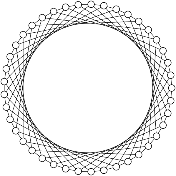
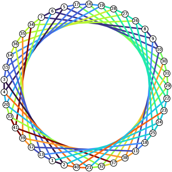
Graph Random Walk
Record	[CLS]1-2-3-4-5-6-7-8-9#6-10#5-11-12-13#1-14-15#1#3-16-17#3#5-5-10-11-18#9#13-13-14-19#16-16-17-5-6-20#4-21-22-23-24#2-25#1#8#18-8-26#24-27#23-28#19#22-22-29#19-19-14-13-18-11-10-5-17-30#10-31#16#29-29-32#21-33#7#20-7-34#26-35#27-36#12#14#28-28-22-29-31-37#32-32-33-7-6-5-4-20-6-5-4-20-33-32-37-38#11#30-39#12#35-12-11-10-5-4-40#2#21#23-2-24-23-27-28-19-16-17-30-10-5-4-40-2-3-4-5-17-3-2-40-4-20-33-32-21-20-33-41#34#37#39-39-38-37-31-29-32-33-41-34-35-36-28-27-35-39-12-13-1-15-3-4-20-6-7-33-41-34-35-39-41-37-32-33-20-21-40-23-22-29-31-37-41-34-35-39-12-13-18-25-24-26-34-7-33-20-4-40-23-27-35-36-12-11-10-30-31-16-15-3-4-40-23-22-28-36-14-19-29-31-37-41-33-32-29-22-21-32-33-20-4-40-21-22-29-19-14-15-16-31-29-[SEP]
Answer	csl(41, 9)
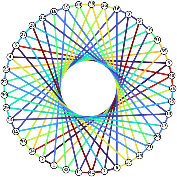
Graph Random Walk
Record	[CLS]1-2-3-4-5-6-7-8-9-10-11-12-13-14#8-15-16#6#8-6-7-8-14-13-17-18#12-19#1-20#17-21-22-23#4-24#21-21-20-17-13-25#15-26-27#5#7-28#12#25-12-13-14-29#9#17-17-13-25-28-12-13-14-8-9-10-30#20#22#29-22-31#10-32#1#11#18-1-19-33#2#21-21-22-31-32-1-19-33-2-34-35#15#26-36#16-16-15-25-28-27-7-6-37#4#24#36-4-23-24-38#33#34#36-34-2-1-39#3#23#31-23-24-38-33-19-1-2-3-39-23-24-21-33-38-24-23-4-37-24-23-39-1-2-34-38-36-37-6-5-4-23-39-3-4-5-6-16-15-35-26-40#3#5#34-5-6-7-27-28-12-13-17-29-9-41#7#11#28-7-27-26-25-13-12-11-32-18-12-13-14-15-25-26-40-34-38-36-37-24-23-4-37-24-21-33-2-3-4-5-27-7-6-16-15-35-34-2-3-40-26-35-34-38-33-21-20-17-29-14-15-16-8-9-41-28-27-7-8-14-15-25-28-27-5-6-7-41-9-8-7-41-9-10-31-[SEP]
Answer	csl(41, 16)

Figure 2: Two CSL graphs and text records of random walks from Algorithms 1 and 3. Task is graph classification into 10 isomorphism types $\mathrm{csl}(41,s)$ for skip length $s\in\{2,3,4,5,6,9,11,12,13,16\}$. In random walks, we label vertices by anonymization and color edges by their time of discovery.

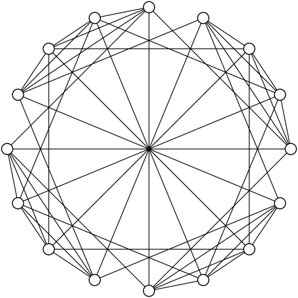
Graph Random Walk
Record	[CLS]1-2-3-4#2-5-6-7#1#2#5-8#3#5#6-9#3-3-4-5-10#1#4-11#1#3#8#9-12#1#6#10-13#6#9-6-5-8-7-2-14#3#4#6#12#13-13-9-15#1#2#7#13-7-6-13-12-1-2-4-10-12-11-1-7-15-1-11-12-10-4-14-13-15-2-7-8-9-3-2-7-8-5-7-2-3-14-13-15-1-2-14-13-16#4#5#9#10#15-5-10-1-11-3-14-4-16-10-1-12-13-6-12-13-6-12-10-11-12-10-11-1-7-6-13-15-16-5-4-14-3-9-13-16-15-1-12-13-9-15-7-2-14-13-6-5-7-2-4-3-9-15-13-14-6-5-7-8-9-11-10-5-16-4-3-14-2-15-13-12-10-5-16-4-14-13-12-14-13-16-10-5-6-14-3-9-16-13-9-15-1-2-15-7-1-12-13-6-8-5-7-6-12-1-11-12-14-4-2-15-9-8-7-1-15-16-4-14-12-1-10-5-16-9-8-5-16-13-12-6-14-2-1-7-15-16-4-2-1-15-16-10-4-16-15-9-16-15-13-6-8-9-16-5-6-[SEP]
Answer	$4\times 4$ rook’s graph
Graph Random Walk
Record	[CLS]1-2-3-4#2-5#3-6#1-7#5-8#3#5-9#3-3-4-5-10#1#4#6-11#4#9-12#2#4#7-13#6#7#9#11-7-14#1#2#8#12-8-5-6-7-13-9-11-4-5-3-4-12-14-1-10-6-15#1#2#3#9#13-2-14-16#1#8#9#10#11-10-11-4-10-6-1-16-8-7-5-8-9-3-5-7-8-14-7-6-15-2-3-8-14-2-1-16-11-4-10-6-15-13-6-1-16-10-6-1-16-14-12-13-7-12-4-3-2-12-11-4-5-7-13-15-3-5-6-1-15-9-13-11-16-10-6-13-9-11-4-12-7-13-6-7-5-6-1-15-9-11-13-6-5-4-2-3-9-15-1-14-16-1-15-6-7-13-15-1-10-5-3-2-1-16-10-4-11-16-10-5-4-12-11-9-16-11-9-13-12-14-16-1-10-4-11-12-13-6-5-7-12-2-3-5-4-10-6-13-9-8-5-10-16-11-12-2-1-6-10-5-3-9-8-14-16-11-10-5-6-7-12-14-16-11-12-14-1-16-11-10-4-11-13-9-16-8-3-5-8-9-16-14-2-[SEP]
Answer	Shrikhande graph

Figure 3: SR16 graphs and text records of random walks from Algorithms 1 and 3. The task is graph classification into two isomorphism types $\{4\times 4\text{ rook's graph},\text{Shrikhande graph}\}$. In random walks, we label vertices by anonymization and color edges by their time of discovery.

Graph Random Walk
Record	[CLS]1-2-3#1-4#2-5#1#2-6#4-7#1#3-3-8#1#4#5#7-5-9#1#2#7-10#4#7#8-11#1#4#8#9-8-12#1#3#6#7-3-13#2#4#6#7#9#11-2-3-7-6-14#2#5#7#8#13-15#2#3#7#9#10-16#3#5#8#10#14-17#1#6#7#10#11#13#14-13-18#5#8#9#11#12#14#16-19#3#6#9#11#12#13#15#16-9-7-13-11-20#1#2#12#14#15#17#18-21#2#4#6#8#10#11#12#14#15#19-8-7-14-5-22#4#6#7#9#10#12#15#18#20-23#2#3#4#10#12#13#16#17#18#20-13-9-2-21-24#1#2#5#6#9#10#12#16#17#19#23-19-6-24-23-16-3-1-5-8-21-14-2-3-7-8-5-6-7-1-25#3#4#5#6#11#15#16#17#19#20#22-17-1-11-4-3-15-20-2-5-22-12-21-14-7-9-5-4-22-20-25-11-21-8-1-24-17-10-23-18-13-6-4-8-3-7-17-14-20-12-24-16-17-10-21-14-5-4-13-14-7-13-3-8-1-3-7-14-13-2-3-8-18-22-5-[SEP]
Answer	Graph 1
Graph Random Walk
Record	[CLS]1-2-3#1-4#1-5#2-6#2#4-7#2#3#4-3-8#4#5#7-9#3#6-10#1#6-11#1#4#6#7#8-12#2#7#8#10-8-13#7#9#12-14#1#2#3#11#12-15#1#2#3#5#6#8#9#10#13-1-3-16#1#4#7#9#10#13-13-17#1#4#6#9#11#14-18#2#3#6#7#9#10#12-19#3#5#8#9#11#14#17-11-7-20#5#6#10#11#13#14#15#16#19-21#1#2#5#7#13#16#17#18#19-16-13-15-22#1#4#5#8#10#12#13#17#18#21-10-6-18-7-11-23#1#2#5#8#9#10#12#16#19#21-12-8-4-24#2#5#6#9#12#13#14#16#17#23-16-10-23-9-6-5-8-19-3-1-23-8-22-5-2-3-16-25#3#4#5#10#12#14#18#19#20#22#24-14-13-16-1-21-17-1-22-15-3-9-13-16-21-22-15-10-11-4-24-9-6-10-12-14-24-12-8-7-11-20-5-25-20-7-6-4-8-3-16-21-20-13-15-5-19-23-5-6-17-9-6-7-11-4-7-3-8-7-3-16-23-2-1-3-8-5-24-23-[SEP]
Answer	Graph 8

Figure 4: Two SR25 graphs and text records of random walks from Algorithms 1 and 3. The task is graph classification into 15 isomorphism types. In random walks, we label vertices by anonymization and color edges by their time of discovery.

System	A walk on the arXiv citation network will be given. Predict the arXiv CS sub-category Paper 1 belongs to. It is one of the following: Numerical Analysis (cs.NA), Multimedia (cs.MM), Logic in Computer Science (cs.LO), ... Discrete Mathematics (cs.DM). Only respond with the answer, do not say any word or explain.
Record	A walk on arXiv citation network is as follows:
	Paper 1 - Title: Safety guided deep reinforcement learning via online gaussian process estimation, Abstract: An important facet of reinforcement learning (rl) has to do with how the agent goes about exploring the environment. traditional exploration strategies typically focus on efficiency and ignore safety. however, for practical applications, ensuring safety of the agent during exploration is crucial since performing an unsafe action or reaching an unsafe state could result in irreversible damage to the agent. the main challenge of safe exploration is that characterizing the unsafe states and actions... Restart at 1. Paper 1 is cited by 2 - Learning to walk in the real world with minimal human effort, Abstract: Reliable and stable locomotion has been one of the most fundamental challenges for legged robots. deep reinforcement learning (deep rl) has emerged as a promising method for developing such control policies... Restart at 1. Paper 1 cites 3 - Deep q learning from demonstrations, Category: Artificial Intelligence (cs.AI), Abstract: Deep reinforcement learning (rl) has achieved several high profile successes in difficult decision-making problems. however, these algorithms typically require a huge amount of data before they reach... Restart at 1. Paper 1 cites 4 - Constrained policy optimization, Category: Machine Learning (cs.LG), Abstract: For many applications of reinforcement learning it can be more convenient to specify both a reward function and constraints, rather than trying to design behavior through the reward function. for example,... Paper 4 is cited by 2. Paper 4 is cited by 5 - Artificial intelligence values and alignment, Abstract: This paper looks at philosophical questions that arise in the context of ai alignment. it defends three propositions. first, normative and technical aspects of the ai alignment problem are interrelated,... Paper 5 cites 6 - Agi safety literature review, Category: Artificial Intelligence (cs.AI), Abstract: The development of artificial general intelligence (agi) promises to be a major event. along with its many potential benefits, it also raises serious safety concerns (bostrom, 2014). the intention of... Paper 6 is cited by 7 - Modeling agi safety frameworks with causal influence diagrams, Abstract: Proposals for safe agi systems are typically made at the level of frameworks, specifying how the components of the proposed system should be trained and interact with each other. in this paper, we model... Restart at 1. Paper 1 cites 8 - Safe learning of regions of attraction for uncertain nonlinear systems with gaussian processes, Category: Systems and Control (cs.SY), Abstract: Control theory can provide useful insights into the properties of controlled, dynamic systems. one important property of nonlinear systems is the region of attraction (roa), a safe subset of the state... Paper 8 is cited by 9 - Control theory meets pomdps a hybrid systems approach, Abstract: Partially observable markov decision processes (pomdps) provide a modeling framework for a variety of sequential decision making under uncertainty scenarios in artificial intelligence (ai). since the... Restart at 1.
	...
	Which arXiv CS sub-category does Paper 1 belong to? Only respond with the answer, do not say any word or explain.
Answer	Machine Learning (cs.LG)

Figure 5: Transductive classification on arXiv citation network using text record of random walk from Algorithms 1 and 4. Colors indicate task instruction, walk information, and label information.

System	Title and abstract of an arXiv paper will be given. Predict the arXiv CS sub-category the paper belongs to. It is one of the following: Numerical Analysis (cs.NA), Multimedia (cs.MM), Logic in Computer Science (cs.LO), ... Discrete Mathematics (cs.DM). Only respond with the answer, do not say any word or explain.
Context	Title: Safety guided deep reinforcement learning via online gaussian process estimation
	Abstract: An important facet of reinforcement learning (rl) has to do with how the agent goes about exploring the environment. traditional exploration strategies typically focus on efficiency and ignore safety. however, for practical applications, ensuring safety of the agent during exploration is crucial since performing an unsafe action or reaching an unsafe state could result in irreversible damage to the agent. the main challenge of safe exploration is that characterizing the unsafe states and actions...
	Which arXiv CS sub-category does this paper belong to?
Answer	Machine Learning (cs.LG)

Figure 6: Zero-shot format for vertex classification on arXiv citation network. Task instruction and label information are colored.

System	Title and abstract of an arXiv paper will be given. Predict the arXiv CS sub-category the paper belongs to. It is one of the following: Numerical Analysis (cs.NA), Multimedia (cs.MM), Logic in Computer Science (cs.LO), ... Discrete Mathematics (cs.DM).
Context	Title: Deeptrack learning discriminative feature representations online for robust visual tracking
	Abstract: Deep neural networks, albeit their great success on feature learning in various computer vision tasks, are usually considered as impractical for online visual tracking, because they require very long...
	Category: cs.CV
	Title: Perceived audiovisual quality modelling based on decison trees genetic programming and neural networks...
	Abstract: Our objective is to build machine learning based models that predict audiovisual quality directly from a set of correlated parameters that are extracted from a target quality dataset. we have used the...
	Category: cs.MM
	...
	Title: Safety guided deep reinforcement learning via online gaussian process estimation
	Abstract: An important facet of reinforcement learning (rl) has to do with how the agent goes about exploring the environment. traditional exploration strategies typically focus on efficiency and ignore safety. however, for practical applications, ensuring safety of the agent during exploration is crucial since performing an unsafe action or reaching an unsafe state could result in irreversible damage to the agent. the main challenge of safe exploration is that characterizing the unsafe states and actions...
	Which arXiv CS sub-category does this paper belong to?
Answer	cs.LG

Figure 7: One-shot format for transductive classification on arXiv citation network. 40 labeled examples are given in form of multi-turn dialogue. Task instruction and label information are colored.

A.3 Attention Visualizations

In Figure 8, we show an example of self-attention in the frozen Llama 3 8B model applied to arXiv transductive classification (Section 5.3). We show attention weights on text record of random walk from the generated cs token as query, which is just before finishing the prediction e.g. cs.CV. We color the strongest activation with orange, and do not color values below $1\%$ of it. The model invests a nontrivial amount of attention on walk information such as Paper 1 cites 12, while also making use of titles and labels of labeled vertices. This indicates the model is utilizing the graph structure recorded by the random walk in conjunction with other information to make predictions.

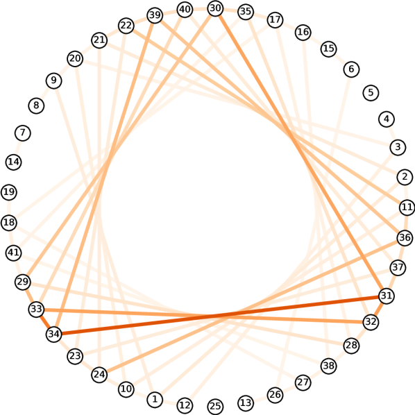
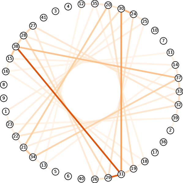
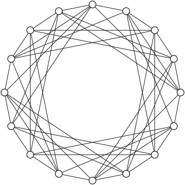
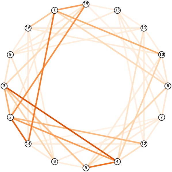
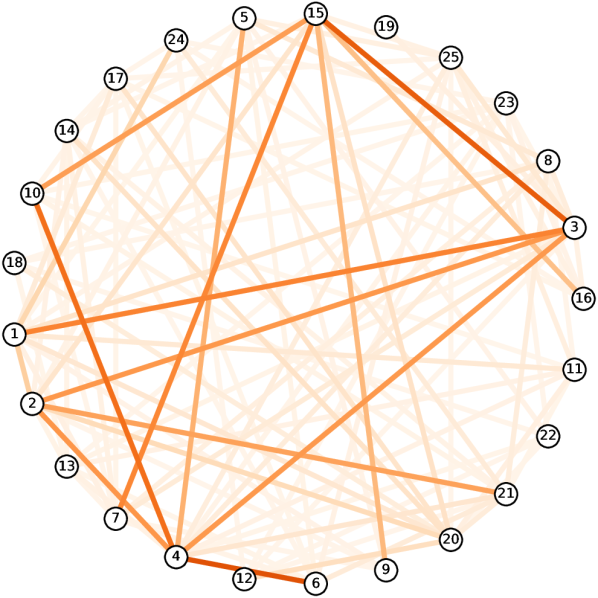
In Figures 9, 10, and 11, we provide examples of self-attention in DeBERTa models trained for graph separation (Section 5.1). We first show attention weights on text record of random walk from the [CLS] query token. Then, we further show an alternative visualization where the attention weights are mapped onto the original input graph. For example, for each attention on $v_{t+1}$ where the walk has traversed $v_{t}\to v_{t+1}$, we regard it as an attention on the edge $(v_{t},v_{t+1})$ in the input graph. We ignore [CLS] and [SEP] tokens since they do not appear on the input graph. We observe that the models often focus on sparse, connected substructures, which presumably provide discriminative information on the isomorphism types. In particular, for CSL graphs (Figure 9) we observe an interpretable pattern of approximate cycles composed of skip links. This is presumably related to measuring the lengths of skip links, which provides sufficient information to infer isomorphism types of CSL graphs.

[…] A walk on arXiv citation network is as follows: Paper 1 - Title: Unsupervised and interpretable scene discovery with discrete attend infer repeat, Abstract: In this work we present discrete attend infer repeat (discrete-air), a recurrent auto-encoder with structured latent distributions containing discrete categorical distributions, continuous attribute distributions, and factorised spatial attention. while inspired by the original air model andretaining air model’s capability in identifying objects in an image, discrete-air provides direct interpretability of the latent codes. we show that for multi-mnist and a multiple-objects version of dsprites... Restart at 1. […] Restart at 1. Paper 1 cites 12 - Attend infer repeat fast scene understanding with generative models, Category: Computer Vision and Pattern Recognition (cs.CV), Abstract: We present a framework for efficient inference in structured image models that explicitly reason about objects. we achieve this by performing probabilistic inference using a recurrent neural network that... Paper 12 cites 3. Paper 12 cites 7. Paper 12 is cited by 9. Paper 12 is cited by 10. Paper 12 cites 11. Restart at 1. Paper 1 cites 11. Restart at 1. Paper 1 cites 12. Paper 12 is cited by 13 - An architecture for deep hierarchical generative models, Category: Machine Learning (cs.LG), Abstract: We present an architecture which lets us train deep, directed generative models with many layers of latent variables. we include deterministic paths between all latent variables and the generated output,... Paper 13 cites 3. Restart at 1. […]
Attention (Layer 13/30)
Answer	cs.CV
Prediction	cs.CV

Figure 8: Example of attention in a frozen Llama 3 8B applied on arXiv transductive classification. Attention weights are averaged over all 30 heads.

1-2-3-4-5-6-7-8#5-9#1#4-1-10-11#2-2-1-12#3#8-3-4-9-8-5-13-14#7-15#6-16-17-18-19#14#16-14-7-8-12-1-9-20#3#10-21#2-22#11-23-24#10#21-10-1-12-25#4#7#13-7-6-5-4-25-12-8-5-4-25-12-8-7-25-13-26#6#19-27#15#18-18-17-28-29-30-31-32#28-33#29-34#23#31-31-32-35#17#30-17-16-19-14-15-6-7-8-5-6-7-8-9-4-3-12-1-10-20-9-8-7-14-19-16-15-6-5-4-9-8-5-4-9-20-21-22-11-36#24-37#23#31-31-34-33-32-28-38#16#27-27-15-16-17-18-27-26-13-25-7-14-19-26-6-15-16-38-27-18-17-35-30-31-34-23-24-21-2-1-10-11-22-39#34#36-40#30#33#37-33-29-30-35-32-33-40-30-35-32-31-37-36-39-34-31-30-29-41#18#35#38-18-27-38-16-17-28-38-27-26-13-14-15-27-26-13-14-15-6-26-13-5-6-15-14-13-25-7-14-15-6-26-27-38-28-29-33-34-39-36-24-10-1-2-

Attention (Head 12/12, Layer 12/12)

Graph Attention Mapped onto Graph

1-2-3-4-5-6#3-7-8-9#1-10#7-7-11#5-5-6-3-4-12-13#5-14#11-15-16#8#11-11-5-13-12-4-5-6-3-4-12-17#8-18#16-19#15-20-21-22-23#1-24-25#1#10-26-27-28-29#24#26-24-25-10-9-1-25-24-30#20#22-31#19#29-29-28-27-32#22-33#21#28-21-34#13-35#12#18#20-12-17-36#2#4#9-9-10-25-26-27-32-22-23-24-25-10-9-8-16-18-19-20-21-34-37#14#33-38#15#28#31-15-14-13-34-21-22-32-39#2#23-2-1-23-24-30-31-38-15-19-31-30-24-29-31-38-15-19-20-35-18-19-15-14-37-34-35-20-21-34-37-33-32-22-21-34-37-33-32-22-30-20-35-18-16-15-14-13-12-35-20-30-22-32-33-37-14-11-5-4-36-2-1-25-26-29-24-23-39-32-22-23-24-25-1-2-36-9-10-25-24-30-31-19-15-16-11-14-37-38-15-14-11-7-10-40#6#26-6-7-10-9-8-17-18-16-11-7-8-16-11-7-8-17-18-16-15-38-37-14-11-5-4-36-17-18-

Attention (Head 5/12, Layer 12/12)

Graph Attention Mapped onto Graph

Figure 9: Examples of attention from [CLS] token in a DeBERTa trained on CSL graph separation, forming approximate cycles using skip links. This is presumably related to measuring the lengths of skip links, which provides sufficient information to infer isomorphism types of CSL graphs.

1-2-3-4#2-5-6-7#1#2#5-8#3#5#6-9#3-3-4-5-10#1#4-11#1#3#8#9-12#1#6#10-13#6#9-6-5-8-7-2-14#3#4#6#12#13-13-9-15#1#2#7#13-7-6-13-12-1-2-4-10-12-11-1-7-15-1-11-12-10-4-14-13-15-2-7-8-9-3-2-7-8-5-7-2-3-14-13-15-1-2-14-13-16#4#5#9#10#15-5-10-1-11-3-14-4-16-10-1-12-13-6-12-13-6-12-10-11-12-10-11-1-7-6-13-15-16-5-4-14-3-9-13-16-15-1-12-13-9-15-7-2-14-13-6-5-7-2-4-3-9-15-13-14-6-5-7-8-9-11-10-5-16-4-3-14-2-15-13-12-10-5-16-4-14-13-12-14-13-16-10-5-6-14-3-9-16-13-9-15-1-2-15-7-1-12-13-6-8-5-7-6-12-1-11-12-14-4-2-15-9-8-7-1-15-16-4-14-12-1-10-5-16-9-8-5-16-13-12-6-14-2-1-7-15-16-4-2-1-15-16-10-4-16-15-9-16-15-13-6-8-9-16-5-6-

Attention (Head 11/12, Layer 10/12)

Graph Attention Mapped onto Graph

1-2-3-4#2-5#3-6#1-7#5-8#3#5-9#3-3-4-5-10#1#4#6-11#4#9-12#2#4#7-13#6#7#9#11-7-14#1#2#8#12-8-5-6-7-13-9-11-4-5-3-4-12-14-1-10-6-15#1#2#3#9#13-2-14-16#1#8#9#10#11-10-11-4-10-6-1-16-8-7-5-8-9-3-5-7-8-14-7-6-15-2-3-8-14-2-1-16-11-4-10-6-15-13-6-1-16-10-6-1-16-14-12-13-7-12-4-3-2-12-11-4-5-7-13-15-3-5-6-1-15-9-13-11-16-10-6-13-9-11-4-12-7-13-6-7-5-6-1-15-9-11-13-6-5-4-2-3-9-15-1-14-16-1-15-6-7-13-15-1-10-5-3-2-1-16-10-4-11-16-10-5-4-12-11-9-16-11-9-13-12-14-16-1-10-4-11-12-13-6-5-7-12-2-3-5-4-10-6-13-9-8-5-10-16-11-12-2-1-6-10-5-3-9-8-14-16-11-10-5-6-7-12-14-16-11-12-14-1-16-11-10-4-11-13-9-16-8-3-5-8-9-16-14-2-

Attention (Head 11/12, Layer 7/12)

Graph Attention Mapped onto Graph

Figure 10: Examples of attention from [CLS] token in a DeBERTa trained on SR16 graph separation. The model tend to focus on neighborhood records that form a sparse connected substructure, which we conjecture to provide discriminative information on the isomorphism type of SR16 graphs.

1-2-3#1-4#2-5#1#2-6#4-7#1#3-3-8#1#4#5#7-5-9#1#2#7-10#4#7#8-11#1#4#8#9-8-12#1#3#6#7-3-13#2#4#6#7#9#11-2-3-7-6-14#2#5#7#8#13-15#2#3#7#9#10-16#3#5#8#10#14-17#1#6#7#10#11#13#14-13-18#5#8#9#11#12#14#16-19#3#6#9#11#12#13#15#16-9-7-13-11-20#1#2#12#14#15#17#18-21#2#4#6#8#10#11#12#14#15#19-8-7-14-5-22#4#6#7#9#10#12#15#18#20-23#2#3#4#10#12#13#16#17#18#20-13-9-2-21-24#1#2#5#6#9#10#12#16#17#19#23-19-6-24-23-16-3-1-5-8-21-14-2-3-7-8-5-6-7-1-25#3#4#5#6#11#15#16#17#19#20#22-17-1-11-4-3-15-20-2-5-22-12-21-14-7-9-5-4-22-20-25-11-21-8-1-24-17-10-23-18-13-6-4-8-3-7-17-14-20-12-24-16-17-10-21-14-5-4-13-14-7-13-3-8-1-3-7-14-13-2-3-8-18-22-5-

Attention (Head 4/12, Layer 9/12)

Graph Attention Mapped onto Graph

1-2-3#1-4#1-5#2-6#2#4-7#2#3#4-3-8#4#5#7-9#3#6-10#1#6-11#1#4#6#7#8-12#2#7#8#10-8-13#7#9#12-14#1#2#3#11#12-15#1#2#3#5#6#8#9#10#13-1-3-16#1#4#7#9#10#13-13-17#1#4#6#9#11#14-18#2#3#6#7#9#10#12-19#3#5#8#9#11#14#17-11-7-20#5#6#10#11#13#14#15#16#19-21#1#2#5#7#13#16#17#18#19-16-13-15-22#1#4#5#8#10#12#13#17#18#21-10-6-18-7-11-23#1#2#5#8#9#10#12#16#19#21-12-8-4-24#2#5#6#9#12#13#14#16#17#23-16-10-23-9-6-5-8-19-3-1-23-8-22-5-2-3-16-25#3#4#5#10#12#14#18#19#20#22#24-14-13-16-1-21-17-1-22-15-3-9-13-16-21-22-15-10-11-4-24-9-6-10-12-14-24-12-8-7-11-20-5-25-20-7-6-4-8-3-16-21-20-13-15-5-19-23-5-6-17-9-6-7-11-4-7-3-8-7-3-16-23-2-1-3-8-5-24-23-

Attention (Head 10/12, Layer 8/12)

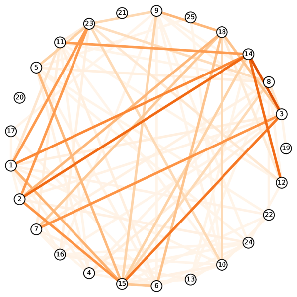
Graph Attention Mapped onto Graph

Figure 11: Examples of attention from [CLS] token in a DeBERTa trained on SR25 graph separation. The model tend to focus on neighborhood records that form a sparse connected substructure, which we conjecture to provide discriminative information on the isomorphism type of SR25 graphs.

A.4 Proofs

We recall that an isomorphism between two graphs $G$ and $H$ is a bijection $\pi:V(G)\to V(H)$ such that any two vertices $u$ and $v$ are adjacent in $G$ if and only if $\pi(u)$ and $\pi(v)$ are adjacent in $H$. If an isomorphism $\pi$ exists between $G$ and $H$, the graphs are isomorphic and written $G\simeq H$ or $G\overset{\pi}{\simeq}H$.

In the proofs, we write by $\mathrm{id}(\cdot)$ the namespace obtained by anonymization of a walk $v_{0}\to\cdots\to v_{l}$ (Section 2.1) that maps each vertex $v_{t}$ to its unique integer name $\mathrm{id}(v_{t})$ starting from $\mathrm{id}(v_{0})=1$.

Let us define some notations related to cover times. These will be used from Appendix A.4.5. We denote by $H(u,v)$ the expected number of steps a random walk starting from $u$ takes until reaching $v$. This is called the hitting time between $u$ and $v$. For a graph $G$, let $C_{V}(G,u)$ be the expected number of steps a random walk starting from $u$ takes until visiting every vertices of $G$. The vertex cover time $C_{V}(G)$, or the cover time, is this quantity given by the worst possible $u$:

$$C_{V}(G)\coloneq\max_{u\in V(G)}C_{V}(G,u).$$ (16)

Likewise, let $C_{E}(G,u)$ be the expected number of steps a random walk starting from $u$ takes until traversing every edge of $G$. The edge cover time $C_{E}(G)$ is given by the worst possible $u$:

$$C_{E}(G)\coloneq\max_{u\in V(G)}C_{E}(G,u).$$ (17)

For local balls $B_{r}(u)$, we always set the starting vertex of the random walk to $u$ (Section 2.2). Thus, we define their cover times as follows:

$$C_{V}(B_{r}(u))\coloneq C_{V}(B_{r}(u),u),$$ (18)

$$C_{E}(B_{r}(u))\coloneq C_{E}(B_{r}(u),u).$$ (19)

A.4.1 Proof of Theorem 2.1 (Section 2.1)

Theorem 2.1.

$X_{\theta}(\cdot)$ is invariant if its random walk algorithm and recording function are invariant.

Proof.

We recall the invariance of a random walk algorithm in Equation (3):

$$\pi(v_{0})\to\cdots\to\pi(v_{l})\overset{d}{=}u_{0}\to\cdots\to u_{l},\quad\forall G\overset{\pi}{\simeq}H,$$ (20)

where $v_{[\cdot]}$ is a random walk on $G$ and $u_{[\cdot]}$ is a random walk on $H$. We further recall the invariance of a recording function $q:(v_{0}\to\cdots\to v_{l},G)\mapsto\mathbf{z}$ in Equation (7):

$$q(v_{0}\to\cdots\to v_{l},G)=q(\pi(v_{0})\to\cdots\to\pi(v_{l}),H),\quad\forall G\overset{\pi}{\simeq}H,$$ (21)

for any given random walk $v_{[\cdot]}$ on $G$. Combining Equation (20) and (21), we have the following:

$$q(v_{0}\to\cdots\to v_{l},G)\overset{d}{=}q(u_{0}\to\cdots\to u_{l},H),\quad\forall G\simeq H.$$ (22)

Then, since the reader neural network $f_{\theta}$ is a deterministic map, we have:

$$f_{\theta}(q(v_{0}\to\cdots\to v_{l},G))\overset{d}{=}f_{\theta}(q(u_{0}\to\cdots\to u_{l},H)),\quad\forall G\simeq H,$$ (23)

which leads to:

$$X_{\theta}(G)\overset{d}{=}X_{\theta}(H),\quad\forall G\simeq H.$$ (24)

This shows Equation (2) and completes the proof. ∎

A.4.2 Proof of Theorem 2.2 (Section 2.1)

We first show a useful lemma.

Lemma A.2.

The random walk in Equation (4) is invariant if the probability distributions of the starting vertex $v_{0}$ and each transition $v_{t-1}\to v_{t}$ are invariant.

Proof.

We prove by induction. Let us write the invariance of the starting vertex $v_{0}$ as follows:

$$\pi(v_{0})\overset{d}{=}u_{0},\quad\forall G\overset{\pi}{\simeq}H,$$ (25)

and the invariance of each transition $v_{t-1}\to v_{t}$ as follows, by fixing $v_{t-1}$ and $u_{t-1}$:

$$\pi(v_{t-1})\to\pi(v_{t})\overset{d}{=}u_{t-1}\to u_{t},\quad\forall G\overset{\pi}{\simeq}H,v_{t-1}\in V(G),u_{t-1}\coloneq\pi(v_{t-1}).$$ (26)

Let us assume the following for some $t\geq 1$:

$$\pi(v_{0})\to\cdots\to\pi(v_{t-1})\overset{d}{=}u_{0}\to\cdots\to u_{t-1},\quad G\overset{\pi}{\simeq}H.$$ (27)

Then, from the chain rule of joint distributions, the first-order Markov property of random walk in Equation (4), and the invariance in Equation (26), we obtain the following:

$$\pi(v_{0})\to\cdots\to\pi(v_{t})\overset{d}{=}u_{0}\to\cdots\to u_{t},\quad G\overset{\pi}{\simeq}H.$$ (28)

By induction from the initial condition $\pi(v_{0})\overset{d}{=}u_{0}$ in Equation (25), the following holds $\forall l>0$:

$$\pi(v_{0})\to\cdots\to\pi(v_{l})\overset{d}{=}u_{0}\to\cdots\to u_{l},\quad\forall G\overset{\pi}{\simeq}H.$$ (29)

This shows Equation (3) and completes the proof. ∎

We now prove Theorem 2.2.

Theorem 2.2.

The random walk in Equation (4) is invariant if its conductance $c_{[\cdot]}(\cdot)$ is invariant:

$$c_{G}(u,v)=c_{H}(\pi(u),\pi(v)),\quad\forall G\overset{\pi}{\simeq}H.$$ (30)

It includes constant conductance, and any choice that only uses degrees of endpoints $\mathrm{deg}(u)$, $\mathrm{deg}(v)$.

Proof.

We recall Equation (4) for a given conductance function $c_{G}:E(G)\to\mathbb{R}_{+}$:

$$\mathrm{Prob}[v_{t}=x|v_{t-1}=u]\coloneq\frac{c_{G}(u,x)}{\sum_{y\in N(u)}c_{G}(u,y)}.$$ (31)

From Lemma A.2, it is sufficient to show the invariance of each transition $v_{t-1}\to v_{t}$ as we sample $v_{0}$ from the invariant distribution $\mathrm{Uniform}(V(G))$ (Algorithm 1). We rewrite Equation (26) as follows:

$$\mathrm{Prob}[v_{t}=x|v_{t-1}=u]=\mathrm{Prob}[u_{t}=\pi(x)|u_{t-1}=\pi(u)],\quad\forall G\overset{\pi}{\simeq}H.$$ (32)

If the conductance function $c_{[\cdot]}(\cdot)$ is invariant (Equation (30)), we can show Equation (32) by:

$$\mathrm{Prob}[v_{t}=x|v_{t-1}=u] \coloneq\frac{c_{G}(u,x)}{\sum_{y\in N(u)}c_{G}(u,y)},$$

$$=\frac{c_{H}(\pi(u),\pi(x))}{\sum_{y\in N(u)}c_{H}(\pi(u),\pi(y))},$$

$$=\frac{c_{H}(\pi(u),\pi(x))}{\sum_{\pi(y)\in N(\pi(u))}c_{H}(\pi(u),\pi(y))},$$

$$=\mathrm{Prob}[u_{t}=\pi(x)|u_{t-1}=\pi(u)],\quad\forall G\overset{\pi}{\simeq}H.$$ (33)

In the third equality, we used the fact that isomorphism $\pi(\cdot)$ preserves adjacency. It is clear that any conductance function $c_{[\cdot]}(\cdot)$ with a constant conductance such as $c_{G}(\cdot)=1$ is invariant. Furthermore, any conductance function that only uses degrees of endpoints $\mathrm{deg}(u)$, $\mathrm{deg}(v)$ is invariant as isomorphism $\pi(\cdot)$ preserves the degree of each vertex. This completes the proof. ∎

A.4.3 Proof of Theorem A.1 (Appendix A.1)

We extend the proof of Theorem 2.2 given in Appendix A.4.2 to second-order random walks discussed in Appendix A.1. We first show a useful lemma:

Lemma A.3.

A second-order random walk algorithm is invariant if the probability distributions of the starting vertex $v_{0}$, the first transition $v_{0}\to v_{1}$, and each transition $(v_{t-2},v_{t-1})\to v_{t}$ for $t>1$ are invariant.

Proof.

We prove by induction. The invariance of starting vertex $v_{0}$ and first transition $v_{0}\to v_{1}$ are:

$$\pi(v_{0}) \overset{d}{=}u_{0},\quad\forall G\overset{\pi}{\simeq}H,$$ (34)

$$\pi(v_{0})\to\pi(v_{1}) \overset{d}{=}u_{0}\to u_{1},\quad\forall G\overset{\pi}{\simeq}H,v_{0}\in V(G),u_{0}\coloneq\pi(v_{0}),$$ (35)

and the invariance of each transition $(v_{t-2},v_{t-1})\to v_{t}$ for $t>1$ can be written as follows by fixing $(v_{t-2},v_{t-1})$ and $(u_{t-2},u_{t-1})$:

$$\pi(v_{t-2})\to\pi(v_{t-1})\to\pi(v_{t})\overset{d}{=}u_{t-2}\to u_{t-1}\to u_{t},\quad \forall G\overset{\pi}{\simeq}H,$$

$$(v_{t-2},v_{t-1})\in E(G),$$

$$(u_{t-2},u_{t-1})\coloneq(\pi(v_{t-2}),\pi(v_{t-1})).$$ (36)

Let us assume the following for some $t\geq 2$:

$$\pi(v_{0})\to\cdots\to\pi(v_{t-2})\to\pi(v_{t-1})\overset{d}{=}u_{0}\to\cdots\to u_{t-2}\to u_{t-1},\quad G\overset{\pi}{\simeq}H.$$ (37)

Then, from the chain rule of joint distributions, the second-order Markov property of second-order random walks, and the invariance in Equation (A.4.3), we obtain the following:

$$\pi(v_{0})\to\cdots\to\pi(v_{t-1})\to\pi(v_{t})\overset{d}{=}u_{0}\to\cdots\to u_{t-1}\to u_{t},\quad G\overset{\pi}{\simeq}H.$$ (38)

By induction from the initial condition $\pi(v_{0})\to\pi(v_{1})\overset{d}{=}u_{0}\to u_{1}$ given from Equations (34) and (35), the following holds $\forall l>0$:

$$\pi(v_{0})\to\cdots\to\pi(v_{l})\overset{d}{=}u_{0}\to\cdots\to u_{l},\quad\forall G\overset{\pi}{\simeq}H.$$ (39)

This shows Equation (3) and completes the proof. ∎

We now prove Theorem A.1.

Theorem A.1.

The non-backtracking random walk in Equation (13) and the node2vec random walk in Equation (14) are invariant if their underlying first-order random walk algorithm is invariant.

Proof.

We assume that the first transition $v_{0}\to v_{1}$ is given by the underlying first-order random walk algorithm. This is true for non-backtracking since there is no $v_{t-2}$ to avoid, and true for the official implementation of node2vec [50]. Then from Lemma A.3, it is sufficient to show the invariance of each transition $(v_{t-2},v_{t-1})\to v_{t}$ for $t>1$ as we sample $v_{0}$ from the invariant distribution $\mathrm{Uniform}(V(G))$ (Algorithm 1) and the first transition $v_{0}\to v_{1}$ is given by the first-order random walk which is assumed to be invariant. We rewrite Equation (A.4.3) as follows:

$$\mathrm{Prob}[v_{t}=x|v_{t-1}=j,v_{t-2}=i]=\mathrm{Prob}[u_{t}=\pi(x)|u_{t-1}=\pi(j),u_{t-2}=\pi(i)],\quad\forall G\overset{\pi}{\simeq}H.$$ (40)

For non-backtracking, we first handle the case where $i\to j$ reaches a dangling vertex $j$ which has $i$ as its only neighbor. In this case the walk begrudgingly backtracks $i\to j\to i$ (Appendix A.1). Since isomorphism $\pi(\cdot)$ preserves adjacency, $\pi(i)\to\pi(j)$ also reaches a dangling vertex $\pi(j)$ and must begrudgingly backtrack $\pi(i)\to\pi(j)\to\pi(i)$. By interpreting the distributions on $v_{t}$ and $u_{t}$ as one-hot at $i$ and $\pi(i)$, respectively, we can see that Equation (40) holds. If $i\to j$ does not reach a dangling vertex, the walk $j\to x$ follows the invariant probability of the underlying first-order random walk $\mathrm{Prob}[v_{t+1}=x|v_{t}=j]$ renormalized over $N(j)\setminus\{i\}$. Then we can show Equation (40) by:

$$\mathrm{Prob}[v_{t}=x |v_{t-1}=j,v_{t-2}=i]$$

$$\coloneq\begin{dcases*}\frac{\mathrm{Prob}[v_{t}=x|v_{t-1}=j]}{\sum_{y\in N(j)\setminus\{i\}}\mathrm{Prob}[v_{t}=y|v_{t-1}=j]}&for $x\neq i$,\\ 0\vphantom{\frac{0}{0}}&for $x=i$,\end{dcases*}$$

$$=\begin{dcases*}\frac{\mathrm{Prob}[u_{t}=\pi(x)|u_{t-1}=\pi(j)]}{\sum_{\pi(y)\in N(\pi(j))\setminus\{\pi(i)\}}\mathrm{Prob}[u_{t}=\pi(y)|u_{t-1}=\pi(j)]}&for $\pi(x)\neq\pi(i)$,\\ 0\vphantom{\frac{0}{0}}&for $\pi(x)=\pi(i)$,\end{dcases*}$$

$$=\mathrm{Prob}[u_{t}=\pi(x)|u_{t-1}=\pi(j),u_{t-2}=\pi(i)],\quad\forall G\overset{\pi}{\simeq}H.$$ (41)

In the second equality, we have used the fact that isomorphism $\pi(\cdot)$ is a bijection and preserves adjacency, and the assumption that the first-order random walk algorithm is invariant. For node2vec random walk, we first show the invariance of the weighting term $\alpha(i,x)$ in Equation (15) using the fact that isomorphism preserves shortest path distances between vertices $d(i,x)=d(\pi(i),\pi(x))$:

$$\alpha(i,x) \coloneq\begin{dcases*}1/p&for $d(i,x)=0$,\\ 1&for $d(i,x)=1$,\\ 1/q&for $d(i,x)=2$.\\ \end{dcases*}$$

$$=\begin{dcases*}1/p&for $d(\pi(i),\pi(x))=0$,\\ 1&for $d(\pi(i),\pi(x))=1$,\\ 1/q&for $d(\pi(i),\pi(x))=2$.\\ \end{dcases*}$$

$$=\alpha(\pi(i),\pi(x)).$$ (42)

Then we can show Equation (40) by:

$$\mathrm{Prob}[v_{t}=x|v_{t-1}=j,v_{t-2}=i] \coloneq\frac{\alpha(i,x)\,\mathrm{Prob}[v_{t}=x|v_{t-1}=j]}{\sum_{y\in N(j)}\alpha(i,y)\,\mathrm{Prob}[v_{t}=y|v_{t-1}=j]},$$

$$=\frac{\alpha(\pi(i),\pi(x))\,\mathrm{Prob}[u_{t}=\pi(x)|u_{t-1}=\pi(j)]}{\sum_{\pi(y)\in N(\pi(j))}\alpha(\pi(i),\pi(y))\,\mathrm{Prob}[u_{t}=\pi(y)|u_{t-1}=\pi(j)]},$$

$$=\mathrm{Prob}[u_{t}=\pi(x)|u_{t-1}=\pi(j),u_{t-2}=\pi(i)],\quad\forall G\overset{\pi}{\simeq}H.$$ (43)

In the second equality, we have used the fact that isomorphism $\pi(\cdot)$ preserves adjacency, and the assumption that the first-order random walk algorithm is invariant. This completes the proof. ∎

A.4.4 Proof of Theorem 2.3 (Section 2.1)

Theorem 2.3.

A recording function $q:(v_{0}\to\cdots\to v_{l},G)\mapsto\mathbf{z}$ that uses anonymization, optionally with named neighborhoods, is invariant.

Proof.

Given a walk $v_{0}\to\cdots\to v_{l}$ on $G$, we can write the anonymized namespace $\mathrm{id}(\cdot)$ as follows:

$$\mathrm{id}(v_{t})=1+\operatorname*{arg\,min}_{i}[v_{i}=v_{t}].$$ (44)

Consider any walk $\pi(v_{0})\to\cdots\to\pi(v_{l})$ on some $H$ which is isomorphic to $G$ via $\pi$. Let us denote the anonymization of this walk as $\mathrm{id}^{\prime}(\cdot)$. Then we have:

$$\mathrm{id}^{\prime}(\pi(v_{t})) =1+\operatorname*{arg\,min}_{i}[\pi(v_{i})=\pi(v_{t})],$$

$$=1+\operatorname*{arg\,min}_{i}[v_{i}=v_{t}],$$

$$=\mathrm{id}(v_{t}),\quad\forall G\overset{\pi}{\simeq}H.$$ (45)

The second equality is due to the fact that $\pi$ is a bijection. This completes the proof for anonymization. For the named neighborhoods, we prove by induction. Let us fix some $t\geq 1$ and assume:

$$q(v_{0}\to\cdots\to v_{t-1},G)=q(\pi(v_{0})\to\cdots\to\pi(v_{t-1}),H),\quad\forall G\overset{\pi}{\simeq}H.$$ (46)

Let $T\subseteq E(G)$ be the set of edges recorded by $\mathbf{z}\coloneq q(v_{0}\to\cdots\to v_{t-1},G)$, and $T^{\prime}\subseteq E(H)$ be the set of edges recorded by $\mathbf{z}^{\prime}\coloneq q(\pi(v_{0})\to\cdots\to\pi(v_{t-1}),H)$. Then, $T$ and $T^{\prime}$ are isomorphic via $\pi$:

$$T^{\prime}=\{(\pi(u),\pi(v))\forall(u,v)\in T\}.$$ (47)

The equality is shown as follows. $(\supseteq)$ Any $(u,v)\in T$ is recorded in $\mathbf{z}$ as $(\mathrm{id}(u),\mathrm{id}(v))$. From Equations (46) and (A.4.4), we have $\mathbf{z}=\mathbf{z}^{\prime}$ and $(\mathrm{id}(u),\mathrm{id}(v))=(\mathrm{id}(\pi(u)),\mathrm{id}(\pi(v)))$. Thus, $(\pi(u),\pi(v))$ is recorded in $\mathbf{z}^{\prime}$ as $(\mathrm{id}(\pi(u)),\mathrm{id}(\pi(v)))$, i.e. $(\pi(u),\pi(v))\in T^{\prime}$. $(\subseteq)$ This follows from symmetry. Now, we choose some $v_{t}\in N(v_{t-1})$ and consider the set $F\subseteq E(G)$ of all unrecorded edges from $v_{t}$:

$$F\coloneq\{(v_{t},u):u\in N(v_{t})\}\setminus T.$$ (48)

Then, the set $D$ of unrecorded neighbors of $v_{t}$ is given as:

$$D\coloneq\{u:(v_{t},u)\in F\}.$$ (49)

Since $\pi(\cdot)$ preserves adjacency, the set $F^{\prime}\subseteq E(H)$ of all unrecorded edges from $\pi(v_{t})$ is given by:

$$F^{\prime} \coloneq\{(\pi(v_{t}),\pi(u)):\pi(u)\in N(\pi(v_{t}))\}\setminus T^{\prime},$$

$$=\{(\pi(v_{t}),\pi(u)):u\in N(v_{t})\}\setminus\{(\pi(u^{\prime}),\pi(v^{\prime}))\forall(u^{\prime},v^{\prime})\in T\},$$

$$=\{(\pi(v_{t}),\pi(u)):u\in N(v_{t}),(v_{t},u)\notin T\},$$

$$=\{(\pi(v_{t}),\pi(u)):(v_{t},u)\in F\},$$ (50)

and consequently:

$$D^{\prime} \coloneq\{\pi(u):(\pi(v_{t}),\pi(u))\in F^{\prime}\},$$

$$=\{\pi(u):u\in D\}.$$ (51)

While $D$ and $D^{\prime}$ may contain vertices not yet visited by the walks and hence not named by $\mathrm{id}(\cdot)$, what we record are named neighbors. Let $S$ be the set of all named vertices in $G$. It is clear that the set $S^{\prime}$ of named vertices in $H$ is given by $S^{\prime}=\{\pi(v):v\in S\}$. Then, the named neighbors in $G$ to be newly recorded for $v_{t-1}\to v_{t}$ is given by $U=D\cap S$, and for $\pi(v_{t-1})\to\pi(v_{t})$ in $H$ the set is given by $U^{\prime}=D^{\prime}\cap S^{\prime}$. Since $\pi(\cdot)$ is a bijection, we can see that $U^{\prime}=\{\pi(u):u\in U\}$. From the invariance of anonymization in Equation (A.4.4), $U$ and $U^{\prime}$ are named identically $\{\mathrm{id}(u):u\in U\}=\{\mathrm{id}(\pi(u)):\pi(u)\in U^{\prime}\}$, and therefore will be recorded identically. As a result, the information to be added to the records at time $t$ are identical, and we have:

$$q(v_{0}\to\cdots\to v_{t},G)=q(\pi(v_{0})\to\cdots\to\pi(v_{t}),H),\quad\forall G\overset{\pi}{\simeq}H.$$ (52)

Then, by induction from the initial condition:

$$q(v_{0},G)=q(\pi(v_{0}),H)=\mathrm{id}(v_{0})=\mathrm{id}(\pi(v_{0}))=1,$$ (53)

the recording function using anonymization and named neighborhoods is invariant. ∎

A.4.5 Proof of Theorem 2.4 (Section 2.2)

Theorem 2.4.

For a uniform random walk on an infinite graph $G$ starting at $v$, the cover time and edge cover time of the finite local ball $B_{r}(v)$ are not always finitely bounded.

Proof.

We revisit the known fact that hitting times on the infinite line $\mathbb{Z}$ is infinite [35, 61, 16, 79]. Consider a local ball $B_{1}(0)$ of radius $1$ from the origin $0$ such that $V(B_{1}(0))=\{-1,0,1\}$. Let us assume that the expected number of steps for a random walk starting at $0$ to visit $1$ for the first time is finite, and denote it by $T$. In the first step of the walk, we have to go either to $-1$ or $1$. If we go to $-1$, we have to get back to $0$ and then to $1$ which would take $2T$ in expectation (by translation symmetry). This leads to $T=1/2\cdot 1+1/2\cdot(1+2T)=1+T$, which is a contradiction. Since visiting all vertices or traversing all edges in in $B_{1}(0)$ clearly involves visiting $1$, the cover time and edge cover time cannot be finitely bounded. ∎

A.4.6 Proof of Theorem 2.5 (Section 2.2)

Let us recall that our graph $G$ is locally finite (Section 2.2), and denote its maximum degree as $\Delta$. We further denote by $d(u,v)$ the shortest path distance between $u$ and $v$. We show some useful lemmas. We first show that $H(u,x)$, the expected number of steps of a random walk starting at $u$ takes until reaching $x$, is finite for any $u$, $x$ in $B_{r}(v)$ for any nonzero restart probability $\alpha$ or restart period $k\geq r$.

Lemma A.4.

For any $u$ and $x$ in $B_{r}(v)$, $H(u,x)$ is bounded by the following:

$$H(u,x)\leq\frac{1}{\alpha}+\frac{1}{\alpha}\left(\frac{\Delta}{1-\alpha}\right)^{r}+\frac{1}{\alpha}\left(\frac{1}{\alpha}-1\right)\left(\frac{\Delta}{1-\alpha}\right)^{2r},$$ (54)

if the random walk restarts at $v$ with any probability $\alpha\in(0,1)$, and:

$$H(u,x)\leq k+k\Delta^{r},$$ (55)

if the random walk restarts at $v$ with any period $k\geq r$.

Proof.

We first prove for random restarts. The proof is inspired by Theorem 1.1 of McNew (2013) [79] and Lemma 2 of Zuckerman (1991) [122]. We clarify some measure-theoretic details. Let $W$ be the set of all (infinite) random walks on $G$. We denote by $P$ the probability measure defined on the space $W$, equipped with its cylinder $\sigma$-algebra, by the random walk restarting at $v$ with probability $\alpha\in(0,1)$. For a vertex $x$ in $G$, we define the hitting time function $|\cdot|_{x}:W\to\mathbb{N}\cup\{\infty\}$ as follows:

$$|w|_{x}\coloneq\operatorname*{arg\,min}_{i}[(w)_{i}=x],\quad\forall w\in W.$$ (56)

Let $W(a)$ be the set of all random walks that start at $a$, $W(a,b)$ be the set of random walks that start at $a$ and visit $b$, and $W(a,b^{-})$ be the set of random walks that start at $a$ and do not visit $b$. Then, the measurability of $|\cdot|_{x}$ follows from the measurability of the sets $W(a)$, $W(a,b)$, and $W(a,b^{-})$, which we show as follows. $\forall a,b\in V(G)$, $W(a)$ is clearly measurable, $W(a,b)$ is measurable as it equals $\bigcup_{n\in\mathbb{N}}\{w\in W|(w)_{1}=a,(w)_{n}=b\}$, and $W(a,b^{-})$ is measurable as it is $W(a)\setminus W(a,b)$.

Consider $W(u,x^{-})$, the set of random walks that start at $u$ and never visit $x$. We start by showing that this set is of measure zero:

$$P(W(u,x^{-}))=0.$$ (57)

For this, we use the fact that $W(u,x^{-})=W(u,v^{-},x^{-})\cup W(u,v,x^{-})$, where $W(u,v^{-},x^{-})$ is the set of random walks starting at $u$ that do not visit $v$ nor $x$, and $W(u,v,x^{-})$ is the set of walks starting at $u$ that visit $v$ and do not visit $x$. We have the following:

$$P(W(u,x^{-})) =P(W(u,v^{-},x^{-}))+P(W(u,v,x^{-})),$$

$$\leq P(W(u,v^{-}))+P(W(u,v,x^{-})).$$ (58)

We show Equation (57) by showing $P(W(u,v^{-}))=0$ and $P(W(u,v,x^{-}))=0$ in Equation (A.4.6).

1. $(P(W(u,v^{-}))=0)$ Consider $W(u,v^{-})$, the set of all random walks that start at $u$ and never visit $v$. Since restart sends a walk to $v$, every walk in this set never restarts. The probability of a walk not restarting until step $t$ is $(1-\alpha)^{t}$. Denote this probability by $p_{t}$, and let $p$ be the probability of a random walk to never restart. Then $p_{t}\downarrow p=0$ and $P(W(u,v^{-}))\leq p=0$.

2. $(P(W(u,v,x^{-}))=0)$ Assume $P(W(u,v,x^{-}))>0$. Then $P(W(v,x^{-}))>0$ since each walk step is independent. Let $W_{N}(v,x^{-})$ be the set of walks that start at $v$ and do not reach $x$ within $N$ restarts. Then we have $W_{N}(v,x^{-})\downarrow W(v,x^{-})$. If a walk restarts at $v$, the probability of reaching $x$ before the next restart is at least the probability of exactly walking the shortest path from $v$ to $x$, which is $\geq(\frac{1-\alpha}{\Delta})^{d(v,x)}\in(0,1)$. Then $P(W_{N}(v,x^{-}))\leq(1-(\frac{1-\alpha}{\Delta})^{d(v,x)})^{N}\downarrow 0$, leading to $P(W(v,x^{-}))=0$. This is a contradiction, so we have $P(W(u,v,x^{-}))=0$.

We are now ready to bound $H(u,x)$. Using the hitting time function $|\cdot|_{x}$ in Equation (56), we have:

$$H(u,x)=\mathbb{E}\left[|w|_{x}|w\in W(u)\right].$$ (59)

Since $W(u)=W(u,x)\cup W(u,x^{-})$, and $P(W(u,x^{-}))=0$ from Equation (57), we have:

$$H(u,x) =\mathbb{E}[|w|_{x}|w\in W(u,x)],$$

$$=\int_{W(u,x)}|w|_{x}\,dP(w|w\in W(u,x)).$$ (60)

Each walk in $W(u,x)$ starts at $u$ and, when it reaches $x$, it either has or has not visited $v$. We treat the two cases separately. Let $W(a,b,c)$ be the set of walks that start at $a$ and reach $c$ after $b$, and let $W(a,b^{-},c)$ be the set of walks that start at $a$ and reach $c$ before $b$. Then we have:

$$H(u,x) =\int_{W(u,v,x)\cup W(u,v^{-},x)}|w|_{x}\,dP(w|W(u,x)),$$

$$=\int_{W(u,v,x)}|w|_{x}\,dP(w|W(u,x))+\int_{W(u,v^{-},x)}|w|_{x}\,dP(w|W(u,x)).$$ (61)

Let $\hat{H}(a,b,c)$ (or $\hat{H}(a,b^{-},c)$) be the expected number of steps for a walk starting at $a$ to reach $c$ after reaching $b$ (or before $b$), given that it is in $W(a,b,c)$ (or in $W(a,b^{-},c)$). If a walk from $u$ reaches $v$ before $x$, the expected steps is given by $\hat{H}(u,x^{-},v)+H(v,x)$. If the walk reaches $x$ before $v$, the expected steps is $\hat{H}(u,v^{-},x)$. Then, if $W(u,v^{-},x)\neq\emptyset$, we can write $H(u,x)$ as follows:

$$H(u,x) =\left[\hat{H}(u,x^{-},v)+H(v,x)\right]P(W(u,v,x)|W(u,x))$$

$$\quad+\hat{H}(u,v^{-},x)\,P(W(u,v^{-},x)|W(u,x)).$$ (62)

On the other hand, if $W(u,v^{-},x)=\emptyset$, we simply have:

$$H(u,x)=\hat{H}(u,x^{-},v)+H(v,x).$$ (63)

We first consider $\hat{H}(u,x^{-},v)$, the expected number of steps from $u$ to reach $v$ before $x$. We show:

$$\hat{H}(u,x^{-},v)\leq\frac{1}{\alpha}.$$ (64)

To see this, note that $\hat{H}(u,x^{-},v)$ is equivalent to the expectation $\mathbb{E}[T]$ of the number of steps $T$ to reach $v$ from $u$, on the graph $G$ with the vertex $x$ deleted and transition probabilities renormalized. If $u$ is isolated on this modified graph, the only walk in $W(u,x^{-},v)$ is the one that immediately restarts at $v$, giving $\mathbb{E}[T]=1$. Otherwise, we have $\mathbb{E}[T]\leq 1/\alpha$ due to the following. Let $T^{\prime}$ be the number of steps until the first restart at $v$. Since restart can be treated as a Bernoulli trial with probability of success $\alpha$, $T^{\prime}$ follows geometric distribution with expectation $1/\alpha$. Since it is possible for the walk to reach $v$ before the first restart, we have $\mathbb{E}[T]\leq\mathbb{E}[T^{\prime}]=1/\alpha$, which gives Equation (64).

We now consider $H(v,x)$, the expectation $\mathbb{E}[T]$ of the number of steps $T$ to reach $x$ from $v$. Let $T^{\prime}$ be the steps until the walk restarts at $v$, then exactly walks the shortest path from $v$ to $x$ for the first time, and then restarts at $v$. Since $T^{\prime}$ walks until restart after walking the shortest path to $x$, and it is possible for a walk to reach $x$ before walking the shortest path to it, we have $\mathbb{E}[T]\leq\mathbb{E}[T^{\prime}]$. Then, we split the walk of length $T^{\prime}$ into $N$ trials, where each trial consists of restarting at $v$ and walking until the next restart. A trial is successful if it immediately walks the shortest path from $v$ to $x$. Then $N$ is the number of trials until we succeed, and it follows geometric distribution with probability of success at least $(\frac{1-\alpha}{\Delta})^{d(v,x)}$ due to bounded degrees. Its expectation is then bounded as:

$$\mathbb{E}[N]\leq\left(\frac{\Delta}{1-\alpha}\right)^{d(v,x)}.$$ (65)

Let $S_{i}$ be the length of the $i$-th trial. Since each $S_{i}$ is i.i.d. with finite mean $\mathbb{E}[S_{i}]=1/\alpha$, and $N$ is stopping time, we can apply Wald’s identity [54] to compute the expectation of $T^{\prime}$:

$$\mathbb{E}[T^{\prime}] =\mathbb{E}[S_{1}+\cdots+S_{N}],$$

$$=\mathbb{E}[N]\mathbb{E}[S_{1}],$$

$$\leq\frac{1}{\alpha}\left(\frac{\Delta}{1-\alpha}\right)^{d(v,x)}.$$ (66)

We remark that $H(v,x)\leq\mathbb{E}[T^{\prime}]$. Combining this result with Equation (64), we have:

$$\hat{H}(u,x^{-},v)+H(v,x)\leq\frac{1}{\alpha}+\frac{1}{\alpha}\left(\frac{\Delta}{1-\alpha}\right)^{d(v,x)}.$$ (67)

If $W(u,v^{-},x)=\emptyset$, we have $H(u,x)=\hat{H}(u,x^{-},v)+H(v,x)$ from Equation (63) and it is finitely bounded for any $\alpha\in(0,1)$ by the above. If $W(u,v^{-},x)\neq\emptyset$, Equations (A.4.6) and (67) lead to:

$$H(u,x) \leq\hat{H}(u,x^{-},v)+H(v,x)+\hat{H}(u,v^{-},x)\,P(W(u,v^{-},x)|W(u,x)),$$

$$\leq\frac{1}{\alpha}+\frac{1}{\alpha}\left(\frac{\Delta}{1-\alpha}\right)^{d(v,x)}+\hat{H}(u,v^{-},x)\,P(W(u,v^{-},x)|W(u,x)),$$ (68)

and it suffices to bound $\hat{H}(u,v^{-},x)\,P(W(u,v^{-},x)|W(u,x))$. We show the following:

$$\hat{H}(u,v^{-},x) =\int_{W(u,v^{-},x)}|w|_{x}\,dP(w|W(u,v^{-},x)),$$

$$=\sum_{k=1}^{\infty}\int_{\{w\in W(u,v^{-},x)\wedge|w|_{x}=k\}}|w|_{x}\,dP(w|W(u,v^{-},x)),$$

$$=\sum_{k=1}^{\infty}k\int_{\{w\in W(u,v^{-},x)\wedge|w|_{x}=k\}}dP(w|W(u,v^{-},x)),$$

$$=\sum_{k=1}^{\infty}k\,P(\{w\in W(u,v^{-},x)\wedge|w|_{x}=k\}|W(u,v^{-},x)),$$

$$\leq\sum_{k=1}^{\infty}k\,P(\{w:|w|_{x}=k\}|W(u,v^{-},x)),$$

$$=\sum_{k=1}^{\infty}k\,\frac{P(\{w:|w|_{x}=k\wedge w\in W(u,v^{-},x)\})}{P(W(u,v^{-},x))},$$

$$\leq\sum_{k=1}^{\infty}k(1-\alpha)^{k}\frac{1}{P(W(u,v^{-},x))},$$

$$=\frac{1}{\alpha}\left(\frac{1}{\alpha}-1\right)\frac{1}{P(W(u,v^{-},x))}.$$ (69)

We have used Fubini’s theorem for the second equality. Then we have:

$$\hat{H}(u,v^{-},x)\,P(W(u,v^{-},x)|W(u,x)) \leq\frac{1}{\alpha}\left(\frac{1}{\alpha}-1\right)\frac{P(W(u,v^{-},x)|W(u,x))}{P(W(u,v^{-},x))},$$

$$=\frac{1}{\alpha}\left(\frac{1}{\alpha}-1\right)\frac{1}{P(W(u,x))}.$$ (70)

$P(W(u,x))$ is at least the probability of precisely walking the shortest path from $u$ to $x$, which has length $d(u,x)\leq 2r$ since $u$ and $x$ are both in $B_{r}(v)$. This gives us the following:

$$P(W(u,x)) \geq\left(\frac{1-\alpha}{\Delta}\right)^{d(u,x)},$$

$$\geq\left(\frac{1-\alpha}{\Delta}\right)^{2r}.$$ (71)

Combining this with Equation (A.4.6), we have:

$$\hat{H}(u,v^{-},x)\,P(W(u,v^{-},x)|W(u,x))\leq\frac{1}{\alpha}\left(\frac{1}{\alpha}-1\right)\left(\frac{\Delta}{1-\alpha}\right)^{2r}.$$ (72)

Combining with Equations (A.4.6) and (67), we have:

$$H(u,x)\leq\frac{1}{\alpha}+\frac{1}{\alpha}\left(\frac{\Delta}{1-\alpha}\right)^{d(v,x)}+\frac{1}{\alpha}\left(\frac{1}{\alpha}-1\right)\left(\frac{\Delta}{1-\alpha}\right)^{2r},$$ (73)

for any $\alpha\in(0,1)$. Notice that, while this bound is for the case $W(u,v^{-},x)\neq\emptyset$, it subsumes the bound for the case $W(u,v^{-},x)=\emptyset$ (Equation (67)). Then, using $d(v,x)\leq r$, we get Equation (54). This completes the proof for random restarts.

We now prove for periodic restarts. If the walk starting at $u$ reaches $x$ before restarting at $v$, the steps taken is clearly less than $k$. If the walk starting at $u$ restarts at $v$ at step $k$ before reaching $x$, it now needs to reach $x$ from $v$, while restarting at $v$ at every $k$ steps. Let $T$ be the steps taken to reach $x$ from $v$. Let $T^{\prime}$ be the number of steps until the walk restarts at $v$, then exactly follows the shortest path from $v$ to $x$ for the first time, and then restarts at $v$. It is clear that $\mathbb{E}[T]\leq\mathbb{E}[T^{\prime}]$. Then, we split the walk of length $T^{\prime}$ into $N$ trials, where each trial consists of restarting at $v$ and walking $k$ steps until the next restart. A trial is successful if it immediately walks the shortest path from $v$ to $x$. Then $N$ is the number of trials until we get a success, and it follows geometric distribution with probability of success at least $(1/\Delta)^{d(v,x)}$ only for $k\geq d(v,x)$, and zero for $k<d(v,x)$ since the walk cannot reach $x$ before restart. Hence, its expectation is at most $\Delta^{d(v,x)}$ for $k\geq d(v,x)$, and we have $\mathbb{E}[T]\leq\mathbb{E}[T^{\prime}]=k\mathbb{E}[N]\leq k\Delta^{d(v,x)}$. Adding the $k$ steps until the first restart at $v$, we have:

$$H(u,x)\leq k+k\Delta^{d(v,x)},$$ (74)

for any $k\geq d(v,x)$. Using $d(v,x)\leq r$, we get Equation (55). This completes the proof. ∎

We now extend Lemma A.4 to edges. Let $H(u,(x,y))$ be the expected number of steps of a random walk starting at $u$ takes until traversing an edge $(x,y)$ by $x\to y$. We show that $H(u,(x,y))$ is finite for any $u$ and adjacent $x$, $y$ in $B_{r}(v)$ for any nonzero restart probability $\alpha$ or restart period $k\geq r+1$.

Lemma A.5.

For any $u$ and adjacent $x$, $y$ in $B_{r}(v)$, $H(u,(x,y))$ is bounded by the following:

$$H(u,(x,y)) \leq\frac{1}{\alpha}+\frac{1}{\alpha}\left(\frac{\Delta}{1-\alpha}\right)^{r+1}+\frac{1}{\alpha}\left(\frac{1}{\alpha}-1\right)\left(\frac{\Delta}{1-\alpha}\right)^{2r+1},$$ (75)

if the random walk restarts at $v$ with any probability $\alpha\in(0,1)$, and:

$$H(u,(x,y)) \leq k+k\Delta^{r+1},$$ (76)

if the random walk restarts at $v$ with any period $k\geq r+1$.

Proof.

The proof is almost identical to Lemma A.4, except the target $x$ of reaching is substituted by $(x,y)$ in the direction of $x\to y$, and all arguments that use the shortest path from $u$ or $v$ to $x$ instead use the shortest path to $x$ postfixed by $x\to y$, which adds $+1$ to several terms in the bounds. ∎

We are now ready to prove Theorem 2.5.

Theorem 2.5.

In Theorem 2.4, if the random walk restarts at $v$ with any nonzero probability $\alpha$ or any period $k\geq r+1$, the cover time and edge cover time of $B_{r}(v)$ are always finite.

Proof.

The proof is inspired by the spanning tree argument of Aleliunas et al. (1979) [4]. Let us consider a depth first search of $B_{r}(v)$ starting from $v$. We denote by $T$ the resulting spanning tree with vertices $V(T)=V(B_{r}(v))$. We consider the expected time for a random walk starting at $v$ to visit every vertex in the precise order visited by the depth first search by traversing each edge twice. It is clear that this upper-bounds the cover time of $B_{r}(v)$ starting at $v$ (Equation (18)):

$$C_{V}(B_{r}(v))\leq\sum_{(x,y)\in E(T)}[H(x,y)+H(y,x)].$$ (77)

Then, using the bounds from Lemma A.4, the property of spanning trees $|E(T)|=|V(T)|-1$, and the fact that $|V(T)|=|V(B_{r}(v))|\leq\Delta^{r}$ from bounded degree, we obtain:

$$C_{V}(B_{r}(v)) \leq 2(\Delta^{r}-1)\left(\frac{1}{\alpha}+\frac{1}{\alpha}\left(\frac{\Delta}{1-\alpha}\right)^{r}+\frac{1}{\alpha}\left(\frac{1}{\alpha}-1\right)\left(\frac{\Delta}{1-\alpha}\right)^{2r}\right),$$ (78)

if the random walk restarts at $v$ with any probability $\alpha\in(0,1)$, and:

$$C_{V}(B_{r}(v)) \leq 2(\Delta^{r}-1)(k+k\Delta^{r}),$$ (79)

if the random walk restarts at $v$ with any period $k\geq r$. This completes the proof for the cover time. For the edge cover time, we consider the expected time for a random walk starting at $v$ to visit every edge in the precise order discovered by the depth first search by traversing each edge twice. It is clear that this upper-bounds the edge cover time of $B_{r}(v)$ starting at $v$ (Equation (19)):

$$C_{E}(B_{r}(v))\leq\sum_{(x,y)\in E(B_{r}(v))}[H(x,(x,y))+H(y,(y,x))].$$ (80)

Then, using Lemma A.4 and the fact that $|E(B_{r}(v))|\leq\Delta^{2r}-1$ from bounded degree, we obtain:

$$C_{E}(B_{r}(v)) \leq 2(\Delta^{2r}-1)\left(\frac{1}{\alpha}+\frac{1}{\alpha}\left(\frac{\Delta}{1-\alpha}\right)^{r+1}+\frac{1}{\alpha}\left(\frac{1}{\alpha}-1\right)\left(\frac{\Delta}{1-\alpha}\right)^{2r+1}\right),$$ (81)

if the random walk restarts at $v$ with any probability $\alpha\in(0,1)$, and:

$$C_{E}(B_{r}(v)) \leq 2(\Delta^{2r}-1)\cdot(k+k\Delta^{r+1}),$$ (82)

if the random walk restarts at $v$ with any period $k\geq r+1$. This completes the proof. ∎

While our proof shows finite bounds for the cover times, it is possible that they can be made tighter, for instance based on Zuckerman (1991) [122]. We leave improving the bounds as a future work.

A.4.7 Proof of Theorem 3.2 (Section 3.1)

We recall universal approximation of graph-level functions in probability (Definition 3.1):

Definition 3.1.

We say $X_{\theta}(\cdot)$ is a universal approximator of graph-level functions in probability if, for all invariant functions $\phi:\mathbb{G}_{n}\to\mathbb{R}$ for a given $n\geq 1$, and $\forall\epsilon,\delta>0$, there exist choices of length $l$ of the random walk and network parameters $\theta$ such that the following holds:

$$\mathrm{Prob}[|\phi(G)-X_{\theta}(G)|<\epsilon]>1-\delta,\quad\forall G\in\mathbb{G}_{n}.$$ (83)

We remark that a random walk neural network $X_{\theta}(\cdot)$ is composed of a random walk algorithm, a recording function $q:(v_{0}\to\cdots\to v_{l},G)\mapsto\mathbf{z}$, and a reader neural network $f_{\theta}:\mathbf{z}\mapsto\hat{\mathbf{y}}\in\mathbb{R}$.

Intuitively, if the record $\mathbf{z}$ of the random walk always provides complete information of the input graph $G$, we may invoke universal approximation of $f_{\theta}$ to always obtain $|\phi(G)-f_{\theta}(\mathbf{z})|<\epsilon$, and thus $|\phi(G)-X_{\theta}(G)|<\epsilon$. However, this is not always true as the random walk may e.g. fail to visit some vertices of $G$, in which case the record $\mathbf{z}$ would be incomplete. As we show below, this uncertainty leads to the probabilistic bound $>1-\delta$ of the approximation.

Let us denote the collection of all possible random walk records as $\{\mathbf{z}\}\coloneq\mathrm{Range}(q)$, and consider a decoding function $\psi:\{\mathbf{z}\}\to\mathbb{G}_{n}$ that takes the record $\mathbf{z}\coloneq q(v_{0}\to\cdots\to v_{l},G)$ of a given random walk $v_{[\cdot]}$ and outputs the graph $\psi(\mathbf{z})\in\mathbb{G}_{n}$ composed of all recorded vertices $V(H)\coloneq\{\mathrm{id}(v_{t}):v_{t}\in\{v_{0},...,v_{l}\}\}$ and all recorded edges $E(H)\subset V(H)\times V(H)$. We show the following lemma:

Lemma A.6.

Let $G_{\mathbf{z}}$ be the subgraph of $G$ whose vertices and edges are recorded by $\mathbf{z}$. Then the graph $\psi(\mathbf{z})$ decoded from the record $\mathbf{z}$ is isomorphic to $G_{\mathbf{z}}$ through the namespace $\mathrm{id}(\cdot)$:

$$G_{\mathbf{z}}\overset{\mathrm{id}}{\simeq}\psi(\mathbf{z}).$$ (84)

Furthermore, the decoded graph $\psi(\mathbf{z})$ reconstructs $G$ up to isomorphism, that is,

$$G\overset{\mathrm{id}}{\simeq}\psi(\mathbf{z}),$$ (85)

if the recording function $q(\cdot)$ and the random walk $v_{[\cdot]}$ satisfies either of the following:

• $q(\cdot)$ uses anonymization, and $v_{[\cdot]}$ has traversed all edges of $G$.

• $q(\cdot)$ uses anonymization and named neighborhoods, and $v_{[\cdot]}$ has visited all vertices of $G$.

Proof.

Equation (84) is straightforward from the fact that the namespace $\mathrm{id}(\cdot)$ defines a bijection from $V(G_{\mathbf{z}})$ to $[|V(G_{\mathbf{z}})|]$, and the recording function uses names $\mathrm{id}(v_{t})$ to record vertices and edges. Equation (85) is satisfied when all vertices and edges of $G$ have been recorded, i.e. $G_{\mathbf{z}}=G$, which is possible either when the random walk has traversed all edges of $G$, or when it has traversed all vertices of $G$ and named neighborhoods are used to record the induced subgraph $G[V(G)]=G$. ∎

We further remark Markov’s inequality for any nonnegative random variable $T$ and $a>0$:

$$\mathrm{Prob}[T\geq a]\leq\frac{\mathbb{E}[T]}{a}.$$ (86)

We are now ready to prove Theorem 3.2.

Theorem 3.2.

A random walk neural network $X_{\theta}(\cdot)$ with a sufficiently powerful $f_{\theta}$ is a universal approximator of graph-level functions in probability (Definition 3.1) if it satisfies either of the below:

• It uses anonymization to record random walks of lengths $l>C_{E}(G)/\delta$.

• It uses anonymization and named neighborhoods to record walks of lengths $l>C_{V}(G)/\delta$.

Proof.

Instead of directly approximating the target function $\phi:\mathbb{G}_{n}\to\mathbb{R}$, it is convenient to define a proxy target function on random walk records $\phi^{\prime}:\{\mathbf{z}\}\to\mathbb{R}$ where $\{\mathbf{z}\}\coloneq\mathrm{Range}(q)$ as follows:

$$\phi^{\prime}\coloneq\phi\circ\psi,$$ (87)

where $\psi:\{\mathbf{z}\}\to\mathbb{G}_{n}$ is the decoding function of walk records. Then, for a given $\mathbf{z}$, we have:

$$G\simeq\psi(\mathbf{z})\quad\Longrightarrow\quad\phi(G)=\phi^{\prime}(\mathbf{z}),$$ (88)

which is because $\phi$ is an invariant function, so $\phi(G)=\phi(\psi(\mathbf{z}))=\phi\circ\psi(\mathbf{z})=\phi^{\prime}(\mathbf{z})$. Then we have:

$$\mathrm{Prob}[G\simeq\psi(\mathbf{z})]\leq\mathrm{Prob}[|\phi(G)-\phi^{\prime}(\mathbf{z})|=0].$$ (89)

We now invoke universality of $f_{\theta}$ to approximate $\phi^{\prime}$. If $f_{\theta}$ is a universal approximator of functions on its domain $\{\mathbf{z}\}\coloneq\mathrm{Range}(q)$, for any $\epsilon>0$ there exists a choice of $\theta$ such that the below holds:

$$|\phi^{\prime}(\mathbf{z})-f_{\theta}(\mathbf{z})|<\epsilon,\quad\forall\mathbf{z}\in\mathrm{Range}(q).$$ (90)

Combining Equations (89) and (90), we have:

$$\mathrm{Prob}[G\simeq\psi(\mathbf{z})]\leq\mathrm{Prob}[|\phi(G)-\phi^{\prime}(\mathbf{z})|+|\phi^{\prime}(\mathbf{z})-f_{\theta}(\mathbf{z})|<\epsilon].$$ (91)

We remark triangle inequality of distances on $\mathbb{R}$, for a given $\mathbf{z}$:

$$|\phi(G)-f_{\theta}(\mathbf{z})|\leq|\phi(G)-\phi^{\prime}(\mathbf{z})|+|\phi^{\prime}(\mathbf{z})-f_{\theta}(\mathbf{z})|,$$ (92)

which implies, for a given $\mathbf{z}$:

$$|\phi(G)-\phi^{\prime}(\mathbf{z})|+|\phi^{\prime}(\mathbf{z})-f_{\theta}(\mathbf{z})|<\epsilon\quad\Longrightarrow\quad|\phi(G)-f_{\theta}(\mathbf{z})|<\epsilon,$$ (93)

and hence:

$$\mathrm{Prob}[|\phi(G)-\phi^{\prime}(\mathbf{z})|+|\phi^{\prime}(\mathbf{z})-f_{\theta}(\mathbf{z})|<\epsilon]\leq\mathrm{Prob}[|\phi(G)-f_{\theta}(\mathbf{z})|<\epsilon].$$ (94)

Combining Equations (91) and (94), we have:

$$\mathrm{Prob}[|\phi(G)-f_{\theta}(\mathbf{z})|<\epsilon]\geq\mathrm{Prob}[G\simeq\psi(\mathbf{z})],$$ (95)

which can be written as follows:

$$\mathrm{Prob}[|\phi(G)-X_{\theta}(G)|<\epsilon]\geq\mathrm{Prob}[G\simeq\psi(\mathbf{z})].$$ (96)

We now consider the probability of the event $G\simeq\psi(\mathbf{z})$ based on Lemma A.6. We first consider the case where the recording function $q(\cdot)$ uses anonymization. In this case, $G\simeq\psi(\mathbf{z})$ is achieved if the random walk of length $l$ has traversed all edges of $G$. Let $T_{E}(G,v_{0})$ be the number of steps that a random walk starting at $v_{0}$ takes until traversing all edges of $G$. Since the edge cover time $C_{E}(G)$ is its expectation taken at the worst possible starting vertex (Equation (17)), we have the following:

$$\mathbb{E}[T_{E}(G,v_{0})]\leq C_{E}(G),\quad\forall v_{0}\in V(G),$$ (97)

which leads to the following from Markov’s inequality (Equation (86)):

$$\mathrm{Prob}[T_{E}(G,v_{0})<l]\geq 1-\frac{\mathbb{E}[T_{E}(G)]}{l}\geq 1-\frac{C_{E}(G)}{l}.$$ (98)

For a given random walk $v_{0}\to\cdots\to v_{l}$ and its record $\mathbf{z}$, the following holds:

$$T_{E}(G,v_{0})<l\quad\Longrightarrow\quad G\simeq\psi(\mathbf{z}),$$ (99)

which implies the following:

$$\mathrm{Prob}[T_{E}(G,v_{0})<l]\leq\mathrm{Prob}[G\simeq\psi(\mathbf{z})].$$ (100)

Combining Equations (96), (98), and (100), we have:

$$\mathrm{Prob}[|\phi(G)-X_{\theta}(G)|<\epsilon]\geq 1-\frac{C_{E}(G)}{l}.$$ (101)

Therefore, for any $\delta>0$, if we choose $l>C_{E}(G)/\delta$ we would have the following:

$$\mathrm{Prob}[|\phi(G)-X_{\theta}(G)|<\epsilon]>1-\delta.$$ (102)

This completes the proof for anonymization. The proof is identical for the recording function that uses anonymization and named neighborhoods, except that the edge cover time is changed to the cover time $C_{V}(G)$ (Equation (16)). This is because neighborhood recording automatically records the induced subgraph of visited vertices, thus visiting all vertices implies recording all edges, $G[V(G)]=G$. ∎

A.4.8 Proof of Theorem 3.4 (Section 3.1)

Theorem 3.4.

A random walk neural network $X_{\theta}(\cdot)$ with a sufficiently powerful $f_{\theta}$ and any nonzero restart probability $\alpha$ or restart period $k\geq r+1$ is a universal approximator of vertex-level functions in probability (Definition 3.3) if it satisfies either of the below for all $B_{r}(v)\in\mathbb{B}_{r}$:

• It uses anonymization to record random walks of lengths $l>C_{E}(B_{r}(v))/\delta$.

• It uses anonymization and named neighborhoods to record walks of lengths $l>C_{V}(B_{r}(v))/\delta$.

Proof.

The proof is almost identical to Theorem 3.2, except $G\in\mathbb{G}_{n}$ are substituted by $B_{r}(v)\in\mathbb{B}_{r}$, and the decoding function $\psi:\{\mathbf{z}\}\to\mathbb{B}_{r}$ is defined to ignore all recorded vertices $\mathrm{id}(x)$ whose shortest path distance from the starting vertex $\mathrm{id}(v)=\mathrm{id}(v_{0})=1$ exceeds $r$. The latter is necessary to restrict the range of the decoding function $\psi$ to $\mathbb{B}_{r}$. In addition, any nonzero restart probability $\alpha$ or restart period $k\geq r+1$ is sufficient to make the cover times $C_{E}(B_{r}(v))$ and $C_{V}(B_{r}(v))$ finite (Theorem 2.5), thereby guaranteeing the existence of a finite choice of $l$. ∎

A.4.9 Proof of Theorem 3.5 (Section 3.2)

Theorem 3.5.

The simple random walk neural network outputs $\mathbf{h}^{(l)}\to\mathbf{x}^{\top}\boldsymbol{\pi}$ as $l\to\infty$.

Proof.

Since $G$ is connected and non-bipartite, the uniform random walk on it defines an ergodic Markov chain with a unique stationary distribution $\boldsymbol{\pi}$. The limiting frequency of visits on each vertex $v$ is precisely the stationary probability $\boldsymbol{\pi}_{v}$. Since the model reads $\mathbf{x}_{v_{0}}\to\cdots\to\mathbf{x}_{v_{l}}$ by average pooling, the output is given by weighted mean $\sum_{v}\boldsymbol{\pi}_{v}\mathbf{x}_{v}$ which is $\mathbf{x}^{\top}\boldsymbol{\pi}$. ∎

A.4.10 Proof of Theorem 3.6 (Section 3.2)

Theorem 3.6.

Let $\mathbf{h}_{u}^{(l)}$ be output of the simple random walk neural network queried with $u$. Then:

$$\mathbb{E}\left[\left|\frac{\partial\mathbf{h}_{u}^{(l)}}{\partial\mathbf{x}_{v}}\right|\right]=\frac{1}{l+1}\left[\sum_{t=0}^{l}P^{t}\right]_{uv}\to\boldsymbol{\pi}_{v}\quad\text{as}\quad l\to\infty.$$ (103)

Proof.

Since the model reads $\mathbf{x}_{v_{0}}\to\cdots\to\mathbf{x}_{v_{l}}$ by average pooling, the feature Jacobian $|\partial\mathbf{h}_{u}^{(l)}/\partial\mathbf{x}_{v}|$ is given as number of visits to the vertex $v$ in the random walk $v_{0}\to\cdots\to v_{l}$ starting at $v_{0}=u$, divided by length $l+1$. Let us denote the expected number of these visits by $J(u,v,l)$. Let $\mathbbm{1}_{v_{t}=v}$ be the indicator function that equals $1$ if $v_{t}=v$ and $0$ otherwise. Then we can write $J(u,v,l)$ as:

$$J(u,v,l) =\mathbb{E}\left[\sum_{t=0}^{l}\mathbbm{1}_{v_{t}=v}|v_{0}=u\right],$$

$$=\sum_{t=0}^{l}\mathbb{E}[\mathbbm{1}_{v_{t}=v}|v_{0}=u].$$ (104)

We have used linearity of expectations for the second equality. $\mathbb{E}[\mathbbm{1}_{v_{t}=v}|v_{0}=u]$ is the probability of being at $v$ at step $t$ given that the walk started at $u$. This probability is precisely $[P^{t}]_{uv}$. Therefore:

$$J(u,v,l)=\sum_{t=0}^{l}\left[P^{t}\right]_{uv}=\left[\sum_{t=0}^{l}P^{t}\right]_{uv},$$ (105)

which gives the equality in Equation (103). Furthermore, since $G$ is connected and non-bipartite, the uniform random walk on it defines an ergodic Markov chain with a unique stationary distribution $\boldsymbol{\pi}$. The limiting frequency of visits on vertex $v$ is precisely the stationary probability $\boldsymbol{\pi}_{v}$, which gives the convergence in Equation (103). This completes the proof. ∎

References

- [1] R. Abboud, İ. İ. Ceylan, M. Grohe, and T. Lukasiewicz. The surprising power of graph neural networks with random node initialization. In IJCAI, 2021.
- [2] M. Abdullah. The cover time of random walks on graphs. arXiv, 2012.
- [3] M. A. Abdullah, C. Cooper, and M. Draief. Speeding up cover time of sparse graphs using local knowledge. In IWOCA, 2015.
- [4] R. Aleliunas, R. M. Karp, R. J. Lipton, L. Lovász, and C. Rackoff. Random walks, universal traversal sequences, and the complexity of maze problems. In Annual Symposium on Foundations of Computer Science, 1979.
- [5] N. Alon, I. Benjamini, E. Lubetzky, and S. Sodin. Non-backtracking random walks mix faster. Communications in Contemporary Mathematics, 2007.
- [6] N. Alvarez-Gonzalez, A. Kaltenbrunner, and V. Gómez. Improving subgraph-GNNs via edge-level ego-network encodings. Transactions on Machine Learning Research, 2024.
- [7] F. Arrigo, D. J. Higham, and V. Noferini. Non-backtracking pagerank. J. Sci. Comput., 2019.
- [8] M. Balcilar, P. Héroux, B. Gaüzère, P. Vasseur, S. Adam, and P. Honeine. Breaking the limits of message passing graph neural networks. In ICML, 2021.
- [9] P. Barceló, E. V. Kostylev, M. Monet, J. Pérez, J. L. Reutter, and J. P. Silva. The logical expressiveness of graph neural networks. In ICLR, 2020.
- [10] S. K. Bera and C. Seshadhri. How to count triangles, without seeing the whole graph. In KDD, 2020.
- [11] M. Black, Z. Wan, A. Nayyeri, and Y. Wang. Understanding oversquashing in gnns through the lens of effective resistance. In ICML, 2023.
- [12] B. Bloem-Reddy and Y. W. Teh. Probabilistic symmetries and invariant neural networks. J. Mach. Learn. Res., 2020.
- [13] M. M. Bronstein, J. Bruna, T. Cohen, and P. Velickovic. Geometric deep learning: Grids, groups, graphs, geodesics, and gauges. arXiv, 2021.
- [14] T. B. Brown, B. Mann, N. Ryder, M. Subbiah, J. Kaplan, P. Dhariwal, A. Neelakantan, P. Shyam, G. Sastry, A. Askell, S. Agarwal, A. Herbert-Voss, G. Krueger, T. Henighan, R. Child, A. Ramesh, D. M. Ziegler, J. Wu, C. Winter, C. Hesse, M. Chen, E. Sigler, M. Litwin, S. Gray, B. Chess, J. Clark, C. Berner, S. McCandlish, A. Radford, I. Sutskever, and D. Amodei. Language models are few-shot learners. In NeurIPS, 2020.
- [15] E. R. Bussian. Bounding the edge cover time of random walks on graphs. Georgia Institute of Technology, 1996.
- [16] carnage. Expected hitting time for simple random walk from origin to point (x,y) in 2d-integer-grid. MathOverflow, 2012. [Online:] https://mathoverflow.net/questions/112470.
- [17] A. K. Chandra, P. Raghavan, W. L. Ruzzo, R. Smolensky, and P. Tiwari. The electrical resistance of a graph captures its commute and cover times. Comput. Complex., 1997.
- [18] Y. Chen, S. Qian, H. Tang, X. Lai, Z. Liu, S. Han, and J. Jia. Longlora: Efficient fine-tuning of long-context large language models. arXiv, 2023.
- [19] Z. Chen, L. Chen, S. Villar, and J. Bruna. Can graph neural networks count substructures? In NeurIPS, 2020.
- [20] Z. Chen, H. Mao, H. Li, W. Jin, H. Wen, X. Wei, S. Wang, D. Yin, W. Fan, H. Liu, and J. Tang. Exploring the potential of large language models (llms)in learning on graphs. SIGKDD Explor., 2023.
- [21] Z. Chen, S. Villar, L. Chen, and J. Bruna. On the equivalence between graph isomorphism testing and function approximation with gnns. In NeurIPS, 2019.
- [22] M. Chenebaux. graph-walker: Fastest random walks generator on networkx graphs. https://github.com/kerighan/graph-walker, 2020.
- [23] F. Chiericetti, A. Dasgupta, R. Kumar, S. Lattanzi, and T. Sarlós. On sampling nodes in a network. In WWW, 2016.
- [24] D. Coppersmith, U. Feige, and J. B. Shearer. Random walks on regular and irregular graphs. SIAM J. Discret. Math., 1996.
- [25] R. Cornish. Stochastic neural network symmetrisation in markov categories. arXiv, 2024.
- [26] L. Cotta, G. Yehuda, A. Schuster, and C. J. Maddison. Probabilistic invariant learning with randomized linear classifiers. In NeurIPS, 2023.
- [27] G. Cybenko. Approximation by superpositions of a sigmoidal function. Math. Control. Signals Syst., 1989.
- [28] A. Dasgupta, R. Kumar, and T. Sarlos. On estimating the average degree. In WWW, 2014.
- [29] R. David and U. Feige. Random walks with the minimum degree local rule have o(n) cover time. SIAM J. Comput., 2018.
- [30] A. B. de Luca and K. Fountoulakis. Simulation of graph algorithms with looped transformers. arXiv, 2024.
- [31] G. Delétang, A. Ruoss, J. Grau-Moya, T. Genewein, L. K. Wenliang, E. Catt, C. Cundy, M. Hutter, S. Legg, J. Veness, and P. A. Ortega. Neural networks and the chomsky hierarchy. In ICLR, 2023.
- [32] K. Devriendt and R. Lambiotte. Discrete curvature on graphs from the effective resistance. Journal of Physics: Complexity, 2022.
- [33] J. Ding, J. R. Lee, and Y. Peres. Cover times, blanket times, and majorizing measures. In Annual ACM symposium on Theory of computing, 2011.
- [34] P. G. Doyle and J. L. Snell. Random walks and electric networks. American Mathematical Soc., 1984.
- [35] I. Dumitriu, P. Tetali, and P. Winkler. On playing golf with two balls. SIAM J. Discret. Math., 2003.
- [36] B. Elesedy. Group symmetry in pac learning. In ICLR workshop on geometrical and topological representation learning, 2022.
- [37] B. Elesedy. Symmetry and Generalisation in Machine Learning. PhD thesis, University of Oxford, 2023.
- [38] W. Falcon. Pytorch lightning. https://github.com/Lightning-AI/lightning, 2019.
- [39] D. Fasino, A. Tonetto, and F. Tudisco. Hitting times for non-backtracking random walks. arXiv, 2021.
- [40] B. Fatemi, J. Halcrow, and B. Perozzi. Talk like a graph: Encoding graphs for large language models. arXiv, 2023.
- [41] U. Feige. A tight upper bound on the cover time for random walks on graphs. Random Struct. Algorithms, 1995.
- [42] M. Fey and J. E. Lenssen. Fast graph representation learning with PyTorch Geometric. In ICLR Workshop on Representation Learning on Graphs and Manifolds, 2019.
- [43] R. Fitzner and R. van der Hofstad. Non-backtracking random walk. Journal of Statistical Physics, 2013.
- [44] J. Gasteiger, A. Bojchevski, and S. Günnemann. Predict then propagate: Graph neural networks meet personalized pagerank. In ICLR, 2019.
- [45] A. Georgakopoulos and P. Winkler. New bounds for edge-cover by random walk. Comb. Probab. Comput., 2014.
- [46] J. Gilmer, S. S. Schoenholz, P. F. Riley, O. Vinyals, and G. E. Dahl. Neural message passing for quantum chemistry. In ICML, 2017.
- [47] F. D. Giovanni, T. K. Rusch, M. M. Bronstein, A. Deac, M. Lackenby, S. Mishra, and P. Velickovic. How does over-squashing affect the power of gnns? arXiv, 2023.
- [48] J. H. Giraldo, K. Skianis, T. Bouwmans, and F. D. Malliaros. On the trade-off between over-smoothing and over-squashing in deep graph neural networks. In CIKM, 2023.
- [49] L. J. Grady. Random walks for image segmentation. IEEE Trans. Pattern Anal. Mach. Intell., 2006.
- [50] A. Grover and J. Leskovec. node2vec: Scalable feature learning for networks. In KDD, 2016.
- [51] W. L. Hamilton, Z. Ying, and J. Leskovec. Inductive representation learning on large graphs. In NeurIPS, 2017.
- [52] P. He, X. Liu, J. Gao, and W. Chen. Deberta: decoding-enhanced bert with disentangled attention. In ICLR, 2021.
- [53] X. He, X. Bresson, T. Laurent, A. Perold, Y. LeCun, and B. Hooi. Harnessing explanations: Llm-to-lm interpreter for enhanced text-attributed graph representation learning. In ICLR, 2023.
- [54] J. Hein. Wald’s identity.
- [55] K. Hornik, M. B. Stinchcombe, and H. White. Multilayer feedforward networks are universal approximators. Neural Networks, 1989.
- [56] E. J. Hu, Y. Shen, P. Wallis, Z. Allen-Zhu, Y. Li, S. Wang, L. Wang, and W. Chen. Lora: Low-rank adaptation of large language models. In ICLR, 2022.
- [57] W. Hu, M. Fey, M. Zitnik, Y. Dong, H. Ren, B. Liu, M. Catasta, and J. Leskovec. Open graph benchmark: Datasets for machine learning on graphs. In NeurIPS, 2020.
- [58] Q. Huang, H. He, A. Singh, S.-N. Lim, and A. R. Benson. Combining label propagation and simple models out-performs graph neural networks. arXiv, 2020.
- [59] S. Ikeda, I. Kubo, and M. Yamashita. The hitting and cover times of random walks on finite graphs using local degree information. Theor. Comput. Sci., 2009.
- [60] S. Ivanov and E. Burnaev. Anonymous walk embeddings. In ICML, 2018.
- [61] S. Janson and Y. Peres. Hitting times for random walks with restarts. SIAM J. Discret. Math., 2012.
- [62] J. D. Kahn, N. Linial, N. Nisan, and M. E. Saks. On the cover time of random walks on graphs. Journal of Theoretical Probability, 1989.
- [63] O. Kallenberg et al. Probabilistic symmetries and invariance principles. Springer, 2005.
- [64] M. Kempton. Non-backtracking random walks and a weighted ihara’s theorem. arXiv, 2016.
- [65] J. Kim, D. Nguyen, S. Min, S. Cho, M. Lee, H. Lee, and S. Hong. Pure transformers are powerful graph learners. In NeurIPS, 2022.
- [66] J. Kim, D. Nguyen, A. Suleymanzade, H. An, and S. Hong. Learning probabilistic symmetrization for architecture agnostic equivariance. In NeurIPS, 2023.
- [67] T. N. Kipf and M. Welling. Semi-supervised classification with graph convolutional networks. In ICLR, 2017.
- [68] F. Klubicka, A. Maldonado, A. Mahalunkar, and J. D. Kelleher. Synthetic, yet natural: Properties of wordnet random walk corpora and the impact of rare words on embedding performance. In GWC, 2019.
- [69] F. Klubicka, A. Maldonado, A. Mahalunkar, and J. D. Kelleher. English wordnet random walk pseudo-corpora. In LREC, 2020.
- [70] W. Kwon, Z. Li, S. Zhuang, Y. Sheng, L. Zheng, C. H. Yu, J. E. Gonzalez, H. Zhang, and I. Stoica. Efficient memory management for large language model serving with pagedattention. In Proceedings of the ACM SIGOPS 29th Symposium on Operating Systems Principles, 2023.
- [71] G. Li, M. Müller, B. Ghanem, and V. Koltun. Training graph neural networks with 1000 layers. In ICML, 2021.
- [72] I. Loshchilov and F. Hutter. Decoupled weight decay regularization. In ICLR, 2019.
- [73] A. Loukas. What graph neural networks cannot learn: depth vs width. In ICLR, 2020.
- [74] L. Lovász. Random walks on graphs. Combinatorics, Paul erdos is eighty, 1993.
- [75] K. Lu, A. Grover, P. Abbeel, and I. Mordatch. Frozen pretrained transformers as universal computation engines. In AAAI, 2022.
- [76] C. Lyle, M. van der Wilk, M. Kwiatkowska, Y. Gal, and B. Bloem-Reddy. On the benefits of invariance in neural networks. arXiv, 2020.
- [77] H. Maron, H. Ben-Hamu, H. Serviansky, and Y. Lipman. Provably powerful graph networks. In NeurIPS, 2019.
- [78] K. Martinkus, P. A. Papp, B. Schesch, and R. Wattenhofer. Agent-based graph neural networks. In ICLR, 2023.
- [79] N. McNew. Random walks with restarts, 3 examples, 2013.
- [80] meta llama. llama3: The official meta llama 3 github site. https://github.com/meta-llama, 2024.
- [81] S. Micali and Z. A. Zhu. Reconstructing markov processes from independent and anonymous experiments. Discret. Appl. Math., 2016.
- [82] J. Mitton and R. Murray-Smith. Subgraph permutation equivariant networks. arXiv, 2021.
- [83] C. Morris, M. Ritzert, M. Fey, W. L. Hamilton, J. E. Lenssen, G. Rattan, and M. Grohe. Weisfeiler and leman go neural: Higher-order graph neural networks. In AAAI, 2019.
- [84] R. L. Murphy, B. Srinivasan, V. A. Rao, and B. Ribeiro. Relational pooling for graph representations. In ICML, 2019.
- [85] K. Nguyen, N. M. Hieu, V. D. Nguyen, N. Ho, S. J. Osher, and T. M. Nguyen. Revisiting over-smoothing and over-squashing using ollivier-ricci curvature. In ICML, 2023.
- [86] R. Oliveira. Mixing and hitting times for finite markov chains, 2012.
- [87] Y. Ollivier. Ricci curvature of markov chains on metric spaces. Journal of Functional Analysis, 2009.
- [88] L. Page, S. Brin, R. Motwani, T. Winograd, et al. The pagerank citation ranking: Bringing order to the web, 1999.
- [89] A. Panotopoulou. Bounds for edge-cover by random walks, 2013.
- [90] P. A. Papp, K. Martinkus, L. Faber, and R. Wattenhofer. Dropgnn: Random dropouts increase the expressiveness of graph neural networks. NeurIPS, 2021.
- [91] S. Park, N. Ryu, G. Kim, D. Woo, S.-Y. Yun, and S. Ahn. Non-backtracking graph neural networks. In NeurIPS Workshop: New Frontiers in Graph Learning, 2023.
- [92] A. Paszke, S. Gross, F. Massa, A. Lerer, J. Bradbury, G. Chanan, T. Killeen, Z. Lin, N. Gimelshein, L. Antiga, A. Desmaison, A. Kopf, E. Yang, Z. DeVito, M. Raison, A. Tejani, S. Chilamkurthy, B. Steiner, L. Fang, J. Bai, and S. Chintala. Pytorch: An imperative style, high-performance deep learning library. In NeurIPS, 2019.
- [93] Y. Peres and P. Sousi. Mixing times are hitting times of large sets. Journal of Theoretical Probability, 2015.
- [94] B. Perozzi, R. Al-Rfou, and S. Skiena. Deepwalk: online learning of social representations. In KDD, 2014.
- [95] O. Puny, H. Ben-Hamu, and Y. Lipman. Global attention improves graph networks generalization. arXiv, 2020.
- [96] B. Rappaport, A. Gamage, and S. Aeron. Faster clustering via non-backtracking random walks. arXiv, 2017.
- [97] D. Rothermel, M. Li, T. Rocktäschel, and J. Foerster. Don’t sweep your learning rate under the rug: A closer look at cross-modal transfer of pretrained transformers. arXiv, 2021.
- [98] C. Sanford, B. Fatemi, E. Hall, A. Tsitsulin, M. Kazemi, J. Halcrow, B. Perozzi, and V. Mirrokni. Understanding transformer reasoning capabilities via graph algorithms. arXiv, 2024.
- [99] R. Sato. Training-free graph neural networks and the power of labels as features. arXiv, 2024.
- [100] R. Sato, M. Yamada, and H. Kashima. Random features strengthen graph neural networks. In SDM, 2021.
- [101] Y. Sieradzki, N. Hodos, G. Yehuda, and A. Schuster. Coin flipping neural networks. In ICML, 2022.
- [102] D. Spielman. Spectral and algebraic graph theory. Yale lecture notes, draft of December, 2019.
- [103] B. Tahmasebi, D. Lim, and S. Jegelka. The power of recursion in graph neural networks for counting substructures. In AISTATS, 2023.
- [104] Y. Tan, Z. Zhou, H. Lv, W. Liu, and C. Yang. Walklm: A uniform language model fine-tuning framework for attributed graph embedding. In NeurIPS, 2023.
- [105] J. Tönshoff, M. Ritzert, H. Wolf, and M. Grohe. Walking out of the weisfeiler leman hierarchy: Graph learning beyond message passing. Transactions on Machine Learning Research, 2023.
- [106] J. Topping, F. D. Giovanni, B. P. Chamberlain, X. Dong, and M. M. Bronstein. Understanding over-squashing and bottlenecks on graphs via curvature. In ICLR, 2022.
- [107] H. Touvron, T. Lavril, G. Izacard, X. Martinet, M. Lachaux, T. Lacroix, B. Rozière, N. Goyal, E. Hambro, F. Azhar, A. Rodriguez, A. Joulin, E. Grave, and G. Lample. Llama: Open and efficient foundation language models. arXiv, 2023.
- [108] H. Wang, S. Feng, T. He, Z. Tan, X. Han, and Y. Tsvetkov. Can language models solve graph problems in natural language? In NeurIPS, 2023.
- [109] G. Weiss, Y. Goldberg, and E. Yahav. Thinking like transformers. In M. Meila and T. Zhang, editors, ICML, 2021.
- [110] T. Wolf, L. Debut, V. Sanh, J. Chaumond, C. Delangue, A. Moi, P. Cistac, T. Rault, R. Louf, M. Funtowicz, and J. Brew. Huggingface’s transformers: State-of-the-art natural language processing. arXiv, 2019.
- [111] X. Wu, A. Ajorlou, Z. Wu, and A. Jadbabaie. Demystifying oversmoothing in attention-based graph neural networks. In NeurIPS, 2023.
- [112] K. Xu, W. Hu, J. Leskovec, and S. Jegelka. How powerful are graph neural networks? In ICLR, 2019.
- [113] R. Ye, C. Zhang, R. Wang, S. Xu, and Y. Zhang. Language is all a graph needs. In Findings of EACL, 2024.
- [114] C. Yun, S. Bhojanapalli, A. S. Rawat, S. J. Reddi, and S. Kumar. Are transformers universal approximators of sequence-to-sequence functions? In ICLR, 2020.
- [115] B. Zhang, J. Gai, Y. Du, Q. Ye, D. He, and L. Wang. Beyond weisfeiler-lehman: A quantitative framework for gnn expressiveness. arXiv, 2024.
- [116] J. Zhao, M. Qu, C. Li, H. Yan, Q. Liu, R. Li, X. Xie, and J. Tang. Learning on large-scale text-attributed graphs via variational inference. arXiv, 2022.
- [117] J. Zhao, L. Zhuo, Y. Shen, M. Qu, K. Liu, M. M. Bronstein, Z. Zhu, and J. Tang. Graphtext: Graph reasoning in text space. arXiv, 2023.
- [118] L. Zhao and L. Akoglu. Pairnorm: Tackling oversmoothing in gnns. arXiv, 2019.
- [119] L. Zhao, W. Jin, L. Akoglu, and N. Shah. From stars to subgraphs: Uplifting any GNN with local structure awareness. In ICLR, 2022.
- [120] X. Zhu and Z. Ghahramani. Learning from labeled and unlabeled data with label propagation. ProQuest number: information to all users, 2002.
- [121] X. J. Zhu. Semi-supervised learning literature survey, 2005.
- [122] D. Zuckerman. On the time to traverse all edges of a graph. Inf. Process. Lett., 1991.