Multistage stochastic optimization
of a mono-site hydrogen infrastructure
by decomposition techniques
Abstract
The development of hydrogen infrastructures requires to reduce their costs. In this paper, we develop a multistage stochastic optimization model for the management of a hydrogen infrastructure which consists of an electrolyser, a compressor and a storage to serve a transportation demand. This infrastructure is powered by three different sources: on-site photovoltaic panels (PV), renewable energy through a power purchase agreement (PPA) and the power grid. We consider uncertainties affecting on-site photovoltaic production and hydrogen demand. Renewable energy sources are emphasized in the hydrogen production process to ensure eligibility for a subsidy, which is awarded if the proportion of nonrenewable electricity usage stays under a predetermined threshold. We solve the multistage stochastic optimization problem using a decomposition method based on Lagrange duality. The numerical results indicate that the solution to this problem, formulated as a policy, achieves a small duality gap, thus proving the effectiveness of this approach.
Keywords Hydrogen infrastructure Stochastic optimization Lagrange decomposition
1 Introduction
Hydrogen, a versatile energy carrier, is predominantly produced using fossil fuels, for example through steam methane reforming (SMR) of natural gas, a process that releases significant carbon dioxide (CO2) emissions. As concerns over climate change intensify, there is a growing imperative to shift towards cleaner methods of hydrogen production. Water electrolysis, which generates hydrogen by splitting water molecules using electricity, offers a promising solution. However, the environmental benefits of hydrogen are contingent upon the use of renewable electricity sources.
In addition to environmental considerations, the economic viability of the hydrogen produced by water electrolysis hinges significantly on electricity costs. The cost of electricity represents a significant proportion of the total operational expenses [9], which presents a significant challenge to the widespread adoption of this technology. Thus, optimizing the cost of electricity becomes essential to ensure the competitiveness of hydrogen.
Hydrogen production has several characteristic features. Firstly, the electrolyser, which is the equipment used to produce hydrogen, has a nonlinear electrical consumption given the quantity of hydrogen produced. Typically, the pressure of hydrogen produced by the electrolyser is quite low and since it is the lightest element, a small quantity of it fills up a large space. Therefore, it is customarily compressed and stored at a higher pressure. Furthermore, hydrogen production, which requires electricity, is achieved through an energy mix primarily composed of renewable energy sources. This has led to the recent emergence of various contracts, known as Power Purchase Agreements (PPA), to provide consumers with greater flexibility in producing green hydrogen. However, the optimization of hydrogen production faces significant barriers. Renewable energy sources, such as solar or wind power, while abundant, are characterized by inherent variability and intermittency. Moreover, the uncertainty surrounding hydrogen demand adds complexity to production optimization. Aligning this demand variability with renewable energy intermittency poses a significant challenge in achieving efficient and sustainable hydrogen production.
In the literature related to hydrogen management, a large number of studies incorporates uncertainties in optimization problems by relying on stochastic programming. More precisely, in [8, 10, 3, 12, 13, 5], two-stage stochastic models are proposed where the first stage decision is a design decision concerning the supply chain (equipment sizes, capacities, contracts, etc.) and the second stage is a management decision.
All the previous described works are modeled as two-stage stochastic programming problems, and most of them are numerically solved through the use of mixed integer linear programming solvers (MILP). However, it is worth noting that solving MILP models becomes computationally intractable as the number of scenarios increases. As a result, the operations aspect of the problems are simplified, leading to a representation that may not fully capture the complexity of real-world problems.
Few studies, like [17, 16] rely on multistage stochastic optimization models taking into account nonanticipativity constraints. In [17], a fast backward scenario reduction algorithm [6] is used to derive twenty representative scenarios and then the optimization problem is solved as a MILP. In [16], the hydrogen is produced using renewable energies and is later converted using a fuel cell to satisfy electricity demand. The optimization problem, formulated as a multistage stochastic optimization problem, is solved using Stochastic Dual Dynamic Integer Programming (SDDiP) [18].
To the best of our knowledge, [15] appears to be the most closely aligned with our work. In this study, the authors employ dynamic programming to address a multistage stochastic problem. Their work revolves around hydrogen production utilizing both wind power and grid electricity, with subsequent conversion back into electricity. This process serves the dual purpose of meeting Power Purchase Agreement obligations and potentially generating revenue through grid sales.
In this paper, we formulate and solve a multistage stochastic optimization problem to manage a hydrogen infrastructure. Our contributions are the following.
-
1.
Compared with two-stage stochastic programming models, the proposed model adequately considers the sequential decisions (every hour) with the gradual revealing of the uncertainty over time.
-
2.
The nonlinear electricity consumption of the electrolyser and its functioning modes are taken into consideration.
-
3.
An electricity mix of on-site photovoltaic, renewable electricity through PPA and power grid is used to supply the infrastructure. Renewable energy sources are prioritized in the hydrogen production process to ensure eligibility for a subsidy.
-
4.
Leveraging Lagrange duality, we decompose the original problem into two separate problems. The first one, that we call the operational problem, involves the management of the hydrogen equipment and the demand satisfaction. The second one, that we call the electricity allocation problem, is related to the allocation of the electricity sources.
The paper is organized as follows. In Sect. 2, we describe the studied system. In Sect. 3, we give the problem formulation and propose a method based on Lagrange duality to solve the problem. In Sect. 4, we give the numerical results. Finally, we provide the conclusion of this work in Sect. 5. We relegate proofs and technical points in Appendix.
2 Hydrogen infrastructure management problem
The following work is motivated by a real-life optimization problem proposed by a company. More precisely, we want to take into account in the modeling process that first, the company owns a fleet of diesel trucks and aims to decarbonize it, and second, they have several buildings with large roofs suitable for photovoltaic installations and has been awarded an investment subsidy to help develop green hydrogen infrastructure. In §2.1, we describe the characteristics of the hydrogen infrastructure under study and, in §2.2, we give its mathematical description.
2.1 Hydrogen infrastructure case study
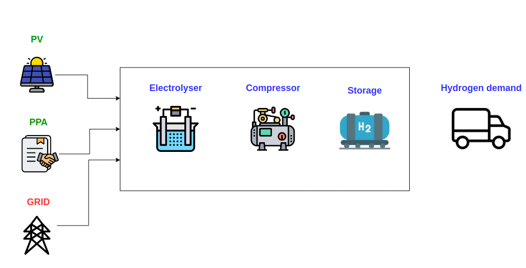
We consider the hydrogen infrastructure described in Figure 1 that is specific to the case study and which is composed of an electrolyser, a compressor that compresses the hydrogen to an adequate pressure and a storage that stores the compressed hydrogen in the same site. This hydrogen infrastructure is powered by solar panels, PPA and the grid to satisfy an uncertain hydrogen demand.
The optimization is done during one week (168 hours), by making decision every hour. Thus, the time horizon is , the set of hours without the time horizon is , the set of hours with the time horizon is and a generic hour is denoted by .
In what follows, we describe the main components of the studied infrastructure: the electricity sources, the electrolyser, the volumetric compressor, the gaseous storage and the hydrogen demand.
2.1.1 Electricity sources
The hydrogen infrastructure is powered by the three following electricity sources.
-
•
Photovoltaic (PV): energy produced from solar radiation through photovoltaic solar panels or power plants. The PV source is costless and its production is uncertain.
-
•
Power Purchase Agreement (PPA): is a long-term contract between an energy producer and a purchaser. This agreement outlines the terms under which the producer will sell electricity to the purchaser. PPAs are widely used in the renewable energy sector to secure financing for projects by providing a stable revenue stream. They mitigate risks for both producers and consumers, ensuring a reliable market for the energy produced. In this case study, we focus on PPA pay as consumed, where the purchaser pays a price per kWh of electricity consumed, rather than a pre-agreed volume, and where, a maximal cumulated quantity of consumed electricity is fixed over a given timespan.
-
•
Grid: electricity available through purchase from the electricity network. In this study, the price of grid electricity is deterministic. Unlike the other two sources, the grid supplies electricity generated from nonrenewable sources.
2.1.2 Electrolyser
An electrolyser is a system made up of “stacks” (of cells) and of a BOP (Balance of plant: rectifier/purifiers for water and gases, etc.). Cell stacks convert chemical energy into electricity, and vice versa, by means of electrochemical reactions involving an anode and a cathode. The electrochemical reaction that produces hydrogen (H2) and oxygen (O2) from water (H2O) occurs in each of the cells of the stacks. The set of possible modes of an electrolyser is denoted by
| (1) |
where the three possible modes are defined as follows.
-
1.
cold: in this mode, the electrolyser is off and does not consume electricity.
-
2.
idle: in this mode, the electrolyser is on and consumes a constant amount of electricity, but does not produce hydrogen. The advantage of being in idle mode is that the electrolyser can quickly switch to the start mode.
-
3.
start: in this mode, the electrolyser is on and is able to produce hydrogen.
All the transitions between two modes are admissible. However, a transition from mode to mode requires a certain amount of time which is assumed to be less than the timestep we consider in the modeling (1 hour). For describing this amount of time, we introduce a function which is such that quantifies the proportion of the current timestep occupied by the transition from to . An example of a function for a specific electrolyser is given in Table 2(b) in §4.1.
The quantity (kg) (used in Equation (9)) is the maximal quantity of hydrogen that the electrolyser can produce during one timestep (hour). The function (used in Equation (5) and (10b)) gives the unitary electricity consumption of the electrolyser, which is the electricity consumption per kilogram of hydrogen produced as a function of the load (quantity of hydrogen produced as a percentage of the maximal hydrogen production). An example of a function for a specific electrolyser is given in Figure 2(a) in §4.1.
2.1.3 Volumetric compressor
A hydrogen volumetric compressor is a device used to increase the pressure of hydrogen gas by reducing its volume through mechanical means, such as piston or diaphragm compression. This process enables the efficient storage and transportation of hydrogen in high-pressure tanks. The quantity (used in Equation (10c)) is the unitary electricity consumption of the compressor per kg of hydrogen produced.
2.1.4 Gaseous storage
Gaseous storage of hydrogen refers to the containment of hydrogen gas under high pressure in specialized tanks or cylinders for use in various applications such as fuel cells, industrial processes, and hydrogen-powered vehicles. Each storage is characterized by its volume, its temperature, and the maximal/minimal possible quantity of hydrogen that can be stored, denoted respectively by and (used Equation (17)).
2.1.5 Hydrogen demand
2.2 Hydrogen infrastructure management modeling
As shown in Figure 1, the operations of this hydrogen infrastructure consist of determining the electricity mix between the uncertain PV, PPA and grid, the mode of the electrolyser and the quantity of hydrogen to produce to satisfy the uncertain hydrogen demand at every hour.
In what follows, we mathematically formulate the hydrogen infrastructure management problem. For this purpose, we introduce decision, state and uncertainty variables, as well as cost functions and constraints.
2.2.1 Decision variables
For every timestep (hour) , the decision variables of the problem are described in Table 1.
| Decision | Description | Domain |
|---|---|---|
| Electricity from PPA (kWh) | ||
| Electricity from the grid (kWh) | ||
| Load at which the electrolyser is functioning | ||
| Turn the electrolyser to cold, idle or start mode | (see (1)) | |
| Quantity of hydrogen extracted from the storage (kg) |
For every timestep (hour) , we gather all decision variables in the control vector
| (2) |
2.2.2 Physical state variables
For every timestep (hour) , we define the physical state variables in Table 2.
| State | Description | Domain |
|---|---|---|
| Quantity of hydrogen in the storage (kg) | ||
| Mode of the electrolyser | (see (1)) |
Economic state variables, that we name cumulative electricity and PPA-stock , will be defined later.
2.2.3 Uncertain variables
For every timestep (hour) , we define the uncertain variables in Table 3.
| Uncertainty | Description | Domain |
|---|---|---|
| Renewable (PV) electricity (kWh) during | ||
| Demand of hydrogen (kg) during |
2.2.4 Cost functions
Hourly cost.
For every timestep (hour) , the instantaneous cost is defined as
| (3) |
where
The electricity cost is split into the PPA cost and the grid cost. The backup cost is linear with respect to the unsatisfied demand, that is, when the quantity is nonnegative and is equal to zero when the demand is satisfied, that is, when .
Subsidy cost.
We also introduce a subsidy cost
| (4) |
where and is the subsidy and is the maximal electricity consumption of the hydrogen infrastructure
| (5) |
The subsidy cost emphasizes the use of renewable energies. Indeed, it is equal to if the cumulated electricity consumption from the grid is less than of the cumulated total electricity consumed (that is, from the grid, PPA and PV). This reflects the fact that a subsidy is granted when renewable sources contribute to more than of the cumulated total electricity consumption.
In the presence of uncertainty, and considering Equation (10a) which will be elaborated upon subsequently, the electrical input from the grid may take negative values when selling excess electricity through the network. However, its impact on the subsidy cost is only accounted when electricity is purchased from the network. Similarly, the sum of PPA electricity and PV electricity supplied to the electrolyser and the compressor might exceed the upper limit of electricity () that can be accepted by the infrastructure. Therefore, the maximum contribution of PPA and PV electricity to the subsidy cost is , as it is delineated in Equation (4) (by employing max and min functions). We rewrite Equation (4) as a function of a sum over to ease the use of Dynamic Programming in §3.2.4
| (6a) | ||||
| where the function is defined by | ||||
| (6b) | ||||
where and is equal to 1 if and 0 otherwise.
We reformulate the subsidy cost in Equation (6) as the final cost , where state , that we name cumulative electricity, has the following dynamics
| (7) |
Summary table.
The parameters used in the instantaneous and subsidy cost functions are described in the following Table 4.
| Variable | Description | Value |
|---|---|---|
| Unitary cost of energy provided by PPA (\euro/kWh) | 0.075\euro/kWh | |
| Unitary cost of energy provided by buying from Grid (\euro/kWh) at timestep h | Figure 3(c) | |
| Unitary cost of not satisfying the hydrogen demand (\euro/kg) | 5,000\euro/kg | |
| Subsidy (\euro) | 5×10⁶\euro | |
| Subsidy threshold | 0.2 | |
| Maximal electricity consumption of the hydrogen infrastructure (kWh) | 1,403 |
2.2.5 Constraints
In this section, we describe the electrolyser, production and electricity constraints, and we give the electrolyser mode and stock dynamics.
Electrolyser constraints.
For every timestep (hour) , the load decision and the decision to change the electrolyser mode are linked one to the other. Indeed, first, if we turn the electrolyser to idle mode (resp. cold mode) by using (resp. ), then the electrolyser cannot produce hydrogen and therefore the load must be equal to zero (. Second, if we turn the electrolyser to start mode, , then the load is to be set in the interval . The coupling constraint, between the load decision and the decision to change the electrolyser mode, is mathematically formalized as follows
| (8) |
Production constraints.
The hydrogen production (in kg) during a time interval , is given by
| (9) |
where is the load decision, the function gives the proportion – expressed in – of the current time interval which is used for hydrogen production when the electrolyser evolves from mode to mode , and is the maximal quantity of hydrogen that the electrolyser can produce during one hour.
The total electricity furnished by the three energy sources is used by both the electrolyser and the compressor, that is
| (10a) | |||
| where the electricity used by the electrolyser is | |||
| (10b) | |||
| and the electricity used by the compressor is | |||
| (10c) | |||
Equation (10a) implies that if the electricity generated by photovoltaic solar panels is high, the surplus is sold to the grid, resulting in taking negative values.
Electricity constraints.
We now describe the electricity constraints. The first and third one are induced constraints derived from Equation (10a). The second one is a constraint induced by the PPA contract.
- •
-
•
The cumulated energy from PPA is upper bounded (as imposed by the contract)
(12) where is the maximal available quantity of PPA electricity during the time horizon.
- •
To ease the use of Dynamic Programming, we reformulate Constraint (12) as , where state , that we name PPA-stock, has the following dynamics
| (14) |
Assuming constraint (14), and noting that is nonnegative for all , it is immediate to see that constraint is equivalent to for all .
Electrolyser mode dynamics.
The dynamics of the mode of the electrolyser is given by
| (15) |
Stock dynamics and constraints.
The dynamics of the stock is given by
| (16) |
where reflects that, if the quantity () extracted from the stock is greater than the demand (), we re-inject the unused quantity of hydrogen in the stock. Moreover, the stock is upper and lower bounded
| (17) |
3 Problem formulation and resolution
In Sect. 2, we have presented the hydrogen infrastructure and given its mathematical modeling. We now turn to formulate an optimization problem corresponding to the management of this infrastructure at minimum cost. In §3.1, we give the problem formulation and, in §3.2, we propose a resolution method based on price decomposition.
3.1 Problem formulation
We consider a probability space . Mathematical expectation is denoted by . Random variables are denoted by bold capital letters like . The -field generated by is denoted by . This notation is used to represent nonanticipativity constraints. All the variables introduced in Sect.2 are now random variables, hence represented by bold letters. We assume that has a given probability distribution with finite support for all .
Gathering all that has been done in Sect.2, we formulate the following minimization problem
| (18a) |
subject to the following constraints for all
| (18b) |
| (18c) |
| (18d) |
| (18e) |
where for every timestep (hour) , the state vector is defined by
| (19) |
The state at initial time, , is deterministic. Now, we comment the different blocks of constraints.
- Operational constraints
- Electricity constraints
- Coupling constraint
- Nonanticipativity constraints
-
The decisions at hour are taken knowing the uncertainties up to hour , which can be written as the first constraint of (18e). Moreover, is observed at the end of hour ; therefore, we require a recourse action to ensure the validity of constraint (18d). For that reason, the decision is taken knowing the uncertainties up to , which can be written as the second constraint of (18e).
Note that the constraints defined in Problem (18) are almost sure constraints, that means they hold for -almost all realizations of the random vector (-a.s.). The solutions of Problem (18) are sequences of hourly policies, that return the optimal decision for each hour given the current state of the infrastructure .
3.2 Resolution using price decomposition
When the random variables are stagewise independent, Dynamic Programming provides an optimal solution to Problem (18). Anyway, without stagewise independence, Dynamic Programming can be used to obtain admissible solution. However, Solving Problem (18) using Dynamic Programming is numerically difficult for the following reasons: one week horizon with hourly decisions gives timesteps; a four dimensional state (see Equation (19)) where the PPA-stock () and the cumulated electricity ( take values in large interval and require a fine discretization which is numerically demanding; five decisions at each hour (see Equation (2)) have to be taken into account in the optimization algorithm.
3.2.1 Sketch of the method
As solving Problem (18) using Dynamic Programming is numerically difficult, we propose an original decomposition method in order to improve numerical tractability with the following steps.
- 1.
-
2.
We make a detour by considering a new additive function , where is a nondecreasing convex proper function, and where, for each value of , is the value of a convex optimization problem which is equivalent (in the sense that the value of the two problems coincide and solutions to either problem can be derived from one another) to the optimization problem whose value is . Moreover, we prove in Proposition 1 that can be chosen in such a way that .
- 3.
-
4.
For each value of , we can build an admissible policy for the original Problem (18) and we can obtain by Monte-Carlo simulation an approximation of the cost associated to that policy denoted by which gives an upper bound of the value of Problem (18). We use this fact to simulate an admissible policy associated to the best obtained at the previous step 3.
3.2.2 Relaxation with deterministic Lagrange multiplier
We observe that Problem (18) is the minimum of the sum of a backup cost and an electricity cost with two different blocks of constraints (LABEL:eq:Schiever_stoch_operational_constraint) and (LABEL:eq:Schiever_stoch_electricity_constraint) (each block having its own variables) and one coupling constraint (18d) for all .
We consider a decomposition algorithm by dualizing the coupling constraint (18d). As constraint (18d) is stochastic, it is natural to dualize with stochastic Lagrange multipliers. However, the optimization over stochastic Lagrange multipliers presents intractability challenges. Therefore, we only consider deterministic Lagrange multipliers. Indeed, we will observe that weak duality is enough to obtain good numerical bounds. We recall that maximizing the stochastic dual function over the restricted set of deterministic multipliers leads to a lower bound of the optimal value of the original problem. The decomposition method is presented now.
Given a deterministic multiplier , we denote by the dual function associated with the final cost of Problem (18)
| (21) | ||||
Note that the final cost is put as a parameter of the dual function for future use and, we denote by Problem -(21) the Problem (21) where the final cost is considered.
By weak duality, the dual function is a lower bound of the value of Problem (18) for all deterministic multiplier
| (22) |
We rewrite the dual function as a sum
| (23a) | ||||
| where the function , which represents what we call the operational problem, is defined for all by | ||||
| (23b) | ||||
| s.t. (LABEL:eq:Schiever_stoch_operational_constraint) , | ||||
| and the function , which represents what we call the electricity allocation problem, is defined for all by | ||||
| (23c) | ||||
| s.t. (LABEL:eq:Schiever_stoch_electricity_constraint) , | ||||
| where for all | ||||
| (23d) | ||||
3.2.3 An equivalent convex electricity allocation problem
The electricity allocation Problem -(23c) obtained by decomposing Problem -(18) is still a challenge for Dynamic Programming as it requires a fine discretization of the two states and . An approximation by a convex optimization problem would enable the use of faster algorithms for its resolution, like Stochastic Dual Dynamic Programming (SDDP) [11], which does not rely on state discretization, and is particularly adapted to the stochastic case.
To obtain a convex approximation of Problem -(23c), we use the two following keys. First, we substitute the nonconvex final cost function with a proper nondecreasing convex function . Second, we replace the cumulative electricity dynamics (nonlinear) as described in Equation (7) with a linear dynamics by introducing new decisions and constraints. The new optimization problem we consider is defined by
| (24a) |
subject to the following constraint,
| (24b) | ||||
| (24c) | ||||
| (24d) |
In (24c), the constraints on model the positive part of in the dynamics of . The constraints on model the min function in the dynamics of .
In Proposition 1, we show that Problem -(23c) and Problem -(24) when considered with the same final cost are equivalent, in the sense that from a feasible solution of Problem -(23c) (resp. Problem -(24)), we can construct a feasible solution for Problem -(24) (resp. Problem -(23c)) that yields the same value. Moreover, we give in Proposition 1 conditions on the choice of to obtain lower bounds on the value of Problem (23c) with the original final cost .
3.2.4 Maximizing the new additive function
In what follows, we assume that satisfies the assumptions of item 3 of Proposition 1, and thus, for any , gives a lower bound of . In order to obtain the best lower bound, we numerically maximize the function using an iterative gradient-like222that is a substitute of the gradient based algorithm whose steps are now detailed.
- Step 1:
-
Initialization of the Lagrange multiplier
In order to choose a good initial value for the Lagrange multiplier, we use a deterministic idealized problem (convex optimization problem) whose optimal solution satisfies certain conditions and for which we are able to find a lower bound for . This is done by applying Lemma 2 for all , which gives us the following lower bounds
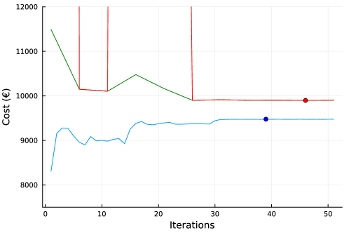
(25) Note that only depends on the parameters of the electricity allocation Problem (23c). We use these lower bounds in our numerical experiments as a starting point to maximize the dual value function . This initialization gives good results as displayed in Figure 4.
- Step 2:
-
Gradient-like based maximization of the dual function
Second, at each iteration of the algorithm, the gradient-like of the function at point is computed using Equation (28). For that purpose, we need to compute the optimal decisions of the operational Problem (23b) and the electricity allocation Problem (23c), which is done as follows.
- Step 2.1:
-
Solving the operational problem
The operational Problem (23b) is solved by Stochastic Dynamic Programming with the pair composed of the stock of hydrogen and the mode of the electrolyser as state variables. The Bellman value functions [1] is given by the following induction. For all for all
(26) where the Bellman value function at time is null. When the random variables are stagewise independent, Dynamic Programming provides an optimal solution.
- Step 2.2:
-
Solving the electricity allocation problem
While Stochastic Dynamic Programming is applicable to the problem, its practical implementation is computationally intensive due to the need for precise discretization of the states and . Alternatively, Stochastic Dual Dynamic Programming (SDDP), leveraging the convex nature of the problem, offers a promising alternative way of obtaining a solution. Note that using the final cost defined in Item 3 of Proposition 1 is preferred when using SDDP, given its polyhedral nature.
The Bellman value functions associated with the electricity allocation Problem (24) are given by the following induction.
At time , we have for all
and for all , for all
(27) Stochastic Dual Dynamic Programming provides lower bounds for the Bellman functions given by the Equations (27).
- Step 2.3:
-
Computation of the gradient of the function
If the function was differentiable, we would obtain that
(28) for all , where is the optimal value of the control of Problems (23b) and (23c) that depend on . Here, as the function is not differentiable (presence of integer controls in Problem (23b)), we use Equation (28) as a gradient-like heuristic to update the multiplier when maximizing the function . The gradient-like is defined by the sum of two expectations. The second one, , is approximated using a Monte-Carlo method while the first one, , is more efficiently computed using the discrete probability law of the state driven by the optimal policy (Fokker-Planck equation).
The algorithm used to maximize using Stochastic Dynamic Programming for the operational Problem (23b) and Stochastic Dual Dynamic Programming for the electricity allocation Problem (23c) is described in Algorithm 1.
3.2.5 Producing an admissible policy
A (state) policy is a mapping from states to controls that determines the action to take at a given time in a given state.
For a fixed deterministic multiplier , we obtain a feasible policy for Problem (18) by considering the following one step optimization problem which uses the sum of the computed Bellman value functions (Step 2.1:) for the operational problem and the lower bounds of the Bellman value functions (27) for the electricity allocation problem
| (29) | ||||
We denote by the total cost of Problem (18) when applying the feasible policy given by Equation (3.2.5).
4 Numerical case study results
4.1 Case study data
We present the different data needed to formulate Problem (18). Some of the data were already presented in Table 4. The optimization problem is formulated at hourly step over one week, thus we have .
-
•
The electrolyser has the following characteristics.
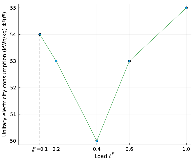
(a) cold idle start cold 1 idle 1 start 1
(b) Figure 2: In (2(a)), we draw the evolution of electricity consumption as a function of the load of the electrolyser and in (2(b)) the values of the function given and -
•
The compressor consumption (used in Equation (10c)) is equal to 6 .
-
•
The minimal capacity of the storage, , is 25 and its maximal capacity, , is 750 (see Equation (17)).
-
•
The electricity sources have the following characteristics.
-
–
The stock of PPA, (used in Equation (12)), is equal to 41,650 .
-
–
The unitary price of PPA (used in Equation (3)) is equal to 0.075\euro/kWh.
-
–
The subsidy is \euro, and the ratio of grid electricity is 0.2 (used in Equation (4)).
-
–
Figure 3(c) shows the time evolution of the grid cost.
-
–
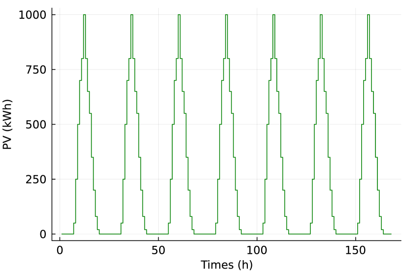
For a given , the PV energy produced during the time interval , , is a random variable with a discrete probability distribution displayed in Table 5, where the set of parameters are given in Figure 3(a).
(a) 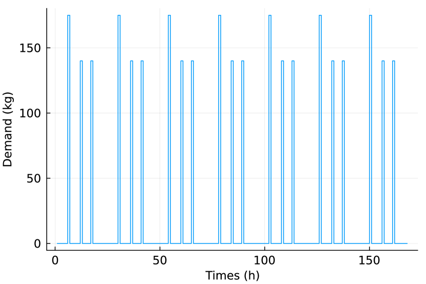
(b) 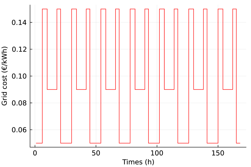
(c) Figure 3: Values of the parameters (a), (b) and the grid cost (c) Table 5: Probability distribution of Outcome 0.8 0.9 1.1 1.2 Probability
-
–
-
•
The hydrogen demand has the following characteristics.
- –
-
–
The dissatisfaction cost is equal to 5,000\euro/kg (see Equation (3)).
Table 6: Probability distribution of Outcome 0.8 0.9 1.1 1.2 Probability
4.2 Implementation of Algorithm 1
Algorithm 1 is implemented in Julia 1.9.2. For the SDP component, we use our own implementation developed in Julia. As for the SDDP component, we employ SDDP.jl as the SDDP solver [2], with SDDP.jl utilizing JuMP [7] as the modeler and Gurobi 11.0 [4] as the LP solver. All computations were performed on a Linux system equipped with 4-processor Intel Xeon E5-2667, 3.30GHz, with 192 GB of RAM.
4.3 Numerical results of Algorithm 1
The value of the parameter is set to 0. The value of parameter is set to 26.5 to penalize grid consumption over 20% of the total electricity consumption. The decisions and and the state are discretized for all for solving the operational Problem (23b) using SDP. In Table 7, we give the bounds and cardinality of the set of discrete values of these variables. The bounds of the variables and are derived from the data of the problem, while the upper bound of is the maximum possible hydrogen demand.
| Variable | Lower bound | Upper bound | Cardinality | |
|---|---|---|---|---|
| =0.1 | 1 | 30 | ||
| (kg) | 0 | 7 | ||
| (kg) | 25 | 750 | 300 |
The SDDP algorithm is iterated 60 times, which is enough to obtain a small duality gap as discussed later. The gradient step is initialized at 5×10⁻⁶ and diminishes by half each 15 iterations across a span of 51 iterations. The number of Monte-Carlo simulation to compute the gradient-like of the function and the total cost using the policy (3.2.5) are 2,300 and 5,000 respectively.
We display in Figure 4 the value of the function at each iteration of Algorithm 1 and the value returned by the policy (3.2.5) when applied to primal problems and each 5 iterations.
As highly penalizes positive values of , it is expected to obtain nonpositive values for when using the policy and therefore to obtain the subsidy . However, during some simulations of the policy before iteration 30, the subsidy is not obtained, leading to the high values observed in the red curve. After iteration 30, takes nonpositive values, and, as the same policy is applied to both problems and , the red and green curves coincide.
4.4 Analysis of some scenarios
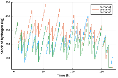
We use the policy (3.2.5) to simulate the evolution of the stock of hydrogen for an initial stock of 250 and for three different scenarios. The evolution of the hydrogen stock is displayed in Figure 5. We note that the hydrogen stock for scenario 2 reaches high values during the first half of the week. This observation implies a low demand for hydrogen within this scenario. Additionally, it suggests that a maximal capacity of at least 500 is required to execute the policy effectively. It is noteworthy that nearly all the hydrogen in the storage is depleted by the end of the horizon for each scenario, which is expected, given the absence of final cost associated with hydrogen stock.
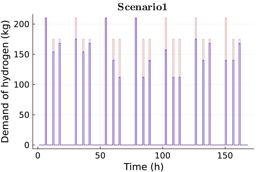
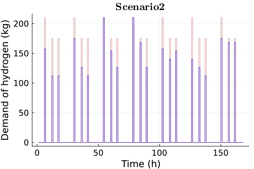
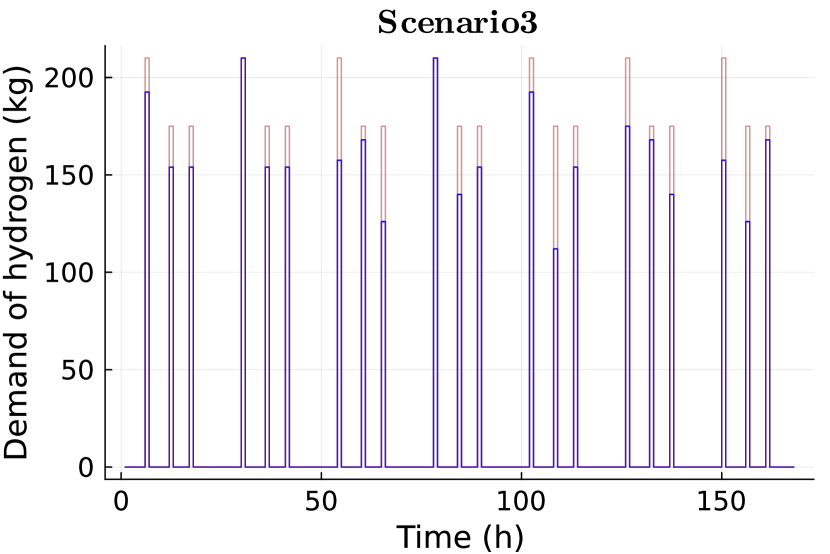
We show in Figure 6 the evolution of the demand and the quantity of hydrogen extracted from the storage to satisfy the hydrogen demand for the three scenarios. As expected, there is low demand during the first half of the week for scenario 2, which explains the large stock of hydrogen during the same period. Note that the demand is always satisfied for every scenario.
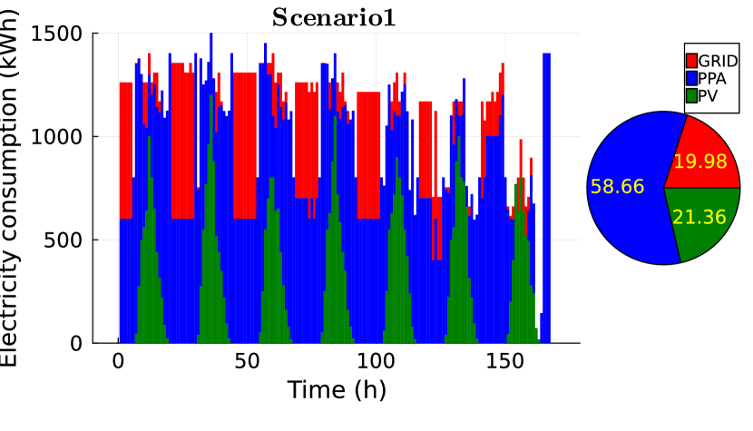
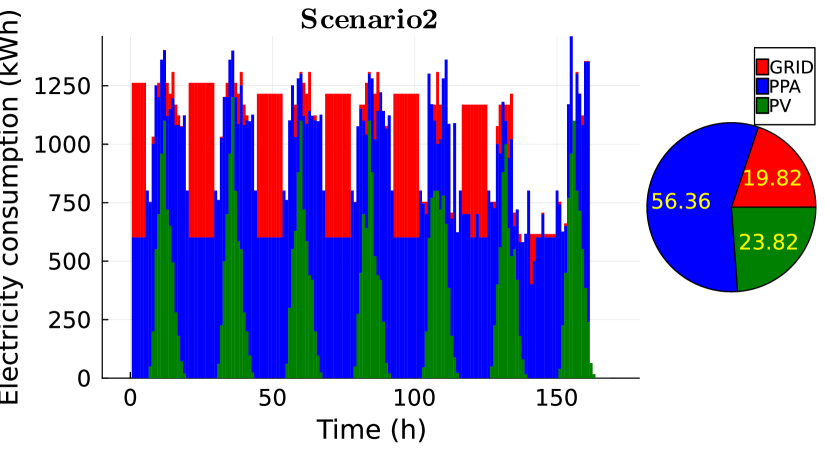
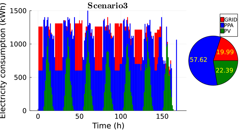
In Figure 7, the electricity consumption is displayed for the three scenarios. We note a pattern where grid electricity is predominantly utilized during the night, taking advantage of its lowest cost. Conversely, PV electricity generation aligns with daytime consumption. For both day and night periods, we complement our energy requirements with PPA. At the end of the week, grid electricity consumption falls below 20 of the total electricity consumption, leading to the acquisition of the subsidy for each scenario.
5 Conclusion
In this study, we have modeled a hydrogen infrastructure consisting of an electrolyser, compressor, and storage. This infrastructure is powered by a mix of electricity sources, namely PV (Photovoltaic), PPA (Power Purchase Agreement) and the grid, and is managed on an hourly basis to meet hydrogen demand. To address the uncertainties in photovoltaic production and hydrogen demand, we formulated the problem as a multistage stochastic optimization problem. Assuming stagewise independence of noise, we have developed a decomposition algorithm mixed with dynamic programming to solve the problem. Our numerical results are encouraging, with the resultant policy achieving a duality gap of 4 . Subsequently, we have analyzed the outcomes of simulations conducted under this policy.
Data Availability
All data used in the numerical experiments is generated as described in this manuscript.
References
- [1] R. Bellman. On the theory of dynamic programming. Proceedings of the National Academy of Sciences, 38(8):716–719, 1952.
- [2] O. Dowson and L. Kapelevich. SDDP.jl: a Julia package for stochastic dual dynamic programming. INFORMS Journal on Computing, 33:27–33, 2021.
- [3] M. Fochesato, P. Heer, and J. Lygeros. Multi-objective optimization of a power-to-hydrogen system for mobility via two-stage stochastic programming. Journal of Physics: Conference Series, 2042:012034, 11 2021.
- [4] Gurobi Optimization, LLC. Gurobi Optimizer Reference Manual, 2023.
- [5] U. Hasturk, A. H. Schrotenboer, K. J. Roodbergen, and E. Ursavas. Multi-period stochastic network design for combined natural gas and hydrogen distribution, 2023.
- [6] H. Heitsch and W. Römisch. Scenario reduction algorithms in stochastic programming. Computational Optimization and Applications, 24(2-3):187 – 206, 2003. Cited by: 739.
- [7] M. Lubin, O. Dowson, J. Dias Garcia, J. Huchette, B. Legat, and J. P. Vielma. JuMP 1.0: Recent improvements to a modeling language for mathematical optimization. Mathematical Programming Computation, 2023.
- [8] U. Mukherjee, A. Maroufmashat, A. Narayan, A. Elkamel, and M. Fowler. A stochastic programming approach for the planning and operation of a power to gas energy hub with multiple energy recovery pathways. Energies, 10, 06 2017.
- [9] H. Nami, O. Rizvandi, C. Chatzichristodoulou, P. Hendriksen, and H. Frandsen. Techno-economic analysis of current and emerging electrolysis technologies for green hydrogen production. Energy Conversion and Management, 269, 2022.
- [10] P. Nunes, F. Oliveira, S. Hamacher, and A. Almansoori. Design of a hydrogen supply chain with uncertainty. International Journal of Hydrogen Energy, 40(46):16408–16418, 2015.
- [11] M. V. Pereira and L. M. Pinto. Multi-stage stochastic optimization applied to energy planning. Math. Program., 52(1-3):359–375, May 2021.
- [12] R. Qi, Y. Qiu, J. Lin, Y. Song, W. Li, X. Xing, and Q. Hu. Two-stage stochastic programming-based capacity optimization for a high-temperature electrolysis system considering dynamic operation strategies. Journal of Energy Storage, 40:102733, 2021.
- [13] A. Rezaee Jordehi, S. A. Mansouri, M. Tostado-Véliz, M. Carrión, M. Hossain, and F. Jurado. A risk-averse two-stage stochastic model for optimal participation of hydrogen fuel stations in electricity markets. International Journal of Hydrogen Energy, 49:188–201, 2024.
- [14] R. T. Rockafellar. Convex analysis. Princeton university press, 2015.
- [15] A. H. Schrotenboer, A. A. Veenstra, M. A. uit het Broek, and E. Ursavas. A green hydrogen energy system: Optimal control strategies for integrated hydrogen storage and power generation with wind energy. Renewable and Sustainable Energy Reviews, 168:112744, 2022.
- [16] X. Sun, X. Cao, M. Li, Q. Zhai, and X. Guan. Seasonal operation planning of hydrogen-enabled multi-energy microgrids through multistage stochastic programming. Journal of Energy Storage, 85:111125, 2024.
- [17] X. Wu, W. Zhao, H. Li, B. Liu, Z. Zhang, and X. Wang. Multi-stage stochastic programming based offering strategy for hydrogen fueling station in joint energy, reserve markets. Renewable Energy, 180:605–615, 2021.
- [18] J. Zou, S. Ahmed, and X. A. Sun. Stochastic dual dynamic integer programming. Math. Program., 175(1-2):461–502, 2019.
Appendix A Proof of Proposition 1
A.1 Proof of item 1 of Proposition 1
We start by preliminary notations and results. First, we consider a sequence , , , admissible for the Problem -(23c). It is straightforward to check that the derived sequence denoted by and defined by
| (30) |
is admissible for Problem -(24). Moreover, as the respective costs of Problem - (23c) and Problem -(24) have the same expression only depending on the sequence , we obtain that the two sequence gives the same cost
| (31) |
Second, we consider a sequence admissible for Problem -(24). We build the sequence defined, for all by
| (32) |
and denote by the sequence
| (33) |
We straightforwardly check that the derived sequence is admissible for Problem -(24) and gives a lower cost. Indeed, it follows from Equation (32) and (24c) that which combined with the fact that the function is nondecreasing gives a lower cost for the derived sequence. Moreover, using the first part, we also have that is admissible for Problem -(23c) with the same cost as the one given by in Problem -(24).
Now, we turn to the proof of item 1 of Proposition 1. We denote by (resp ) the cost function of Problem -(23c) (resp. Problem -(24)).
We consider and assume that , the optimal cost of Problem -(23c), is finite. For , consider a -optimal solution of Problem -(23c). Using the preliminary part, we have that
which gives that and therefore . Now, first assume that is finite and consider a -optimal solution for Problem -(24). We obtain that
which gives the equality . Second, it remains to consider the case . For each we can find an admissible for Problem -(23c) satisfying and proceeding as above we for all which contradict the assumption that is finite.
The cases can be treated in a similar way and are left to the reader.
A.2 Proof of item 2 of Proposition 1
Proof. Fix and consider the optimization Problem (23c). As a preliminary fact, we prove that for a feasible solution of Problem (23c), its component “cumulative electricity” at time satisfies . First, using the cumulative electricity state dynamics (7), we obtain the lower bound
| Second, we obtain the upper bound | ||||
| (as by (11)) | ||||
Now, we prove that . Fix . The optimal cost of Problem (23c) is in as the feasible set of Problem (23c) is bounded, the objective function of Problem (23c) is proper as is proper and has a finite support. Thus, for a given , there exists in the feasible of Problem (23c) satisfying
| (34) |
We immediately obtain that the control is feasible for Problem (23c) where is replaced by . Therefore we have
| (solution feasibility) | ||||
| ( in ) | ||||
| (using (34)) |
We conclude that for all , and therefore that
. Finally, we have
This ends the proof.
A.3 Proof of item 3 of Proposition 1
Proof. First, we prove that Problem (24) is a convex optimization problem. The function is the maximum of affine functions with nonnegative slopes, we conclude that is proper, nondecreasing and convex, which satisfies the assumptions of item 1 of Proposition 1. Consequently, Problem (24) is a convex optimization problem for all .
Appendix B Initialization of Lagrange multiplier
Lemma 2
Let , and be convex functions taking finite values, and be closed convex sets with and , and a sequence of positive parameters. Given , consider the following optimization Problem for all :
| (37a) | ||||
| subject to the following constraints | ||||
| (37b) | ||||
| (37c) | ||||
| (37d) | ||||
| (37e) | ||||
| (37f) | ||||
We assume that if then . We also assume that for , the Lagrangian of Problem (37) when dualizing Constraint (37e) admits a saddle point where is the optimal solution of Problem (37), and is the Lagrange multiplier associated with constraint (37e).
If and then .
Proof.
Assume that and are positive, and choose such that . We construct a solution for Problem (37) with the given , denoted by , in the following manner
It is immediate to see that is feasible for Problem (37) as it differs from only for with , , and . Moreover, we have
and since is feasible for Problem (37), we have
| (38) |
Moreover, as is a convex function [14], we have
In particular, for , we have .
Since is a subgradient of for , it follows that
| (39) |
This ends the proof.