SpectralKAN: Kolmogorov-Arnold Network for Hyperspectral Images Change Detection

Abstract

It has been verified that deep learning methods, including convolutional neural networks (CNNs), graph neural networks (GNNs), and transformers, can accurately extract features from hyperspectral images (HSIs). These algorithms perform exceptionally well on HSIs change detection (HSIs-CD). However, the downside of these impressive results is the enormous number of parameters, FLOPs, GPU memory, training and test times required. In this paper, we propose an spectral Kolmogorov-Arnold Network (KAN) for HSIs-CD (SpectralKAN). SpectralKAN represent a multivariate continuous function with a composition of activation functions to extract HSIs feature and classification. These activation functions are b-spline functions with different parameters that can simulate various functions. In SpectralKAN, a KAN encoder is proposed to enhance computational efficiency for HSIs. And a spatial-spectral KAN encoder is introduced, where the spatial KAN encoder extracts spatial features and compresses the spatial dimensions from patch size to one. The spectral KAN encoder then extracts spectral features and classifies them into changed and unchanged categories. We use five HSIs-CD datasets to verify the effectiveness of SpectralKAN. Experimental verification has shown that SpectralKAN maintains high HSIs-CD accuracy while requiring fewer parameters, FLOPs, GPU memory, training and testing times, thereby increasing the efficiency of HSIs-CD. The code will be available at https://github.com/yanhengwang-heu/SpectralKAN.

I Introduction

Unlike RGB images, hyperspectral images (HSIs) can capture tens to hundreds of finely subdivided spectral bands, ranging from ultraviolet to mid-infrared in the electromagnetic spectrum. Different objects have different spectral curves. Therefore, HSIs processing enables more refined monitoring of the Earth’s surface. HSIs change detection (HSIs-CD) is a technique that obtains land change information by analyzing multi-temporal HSIs at same area. It plays an important role in agriculture and environmental monitoring, land use change, urban planning, and military defense, holding significant research value.

Traditional machine learning methods such as principal component analysis (PCA), support vector machines (SVM), change vector analysis (CVA) [1], and k-means clustering are classic techniques for HSIs-CD [2]. These traditional machine learning methods have low parameters and fast processing speeds, but their ability to extract features from high-dimensional, complex data, likes HSIs, is limited, often resulting in low accuracy.

With the advancement of GPU, the ability of computers to process high-dimensional data has significantly improved. Neural networks have also evolved from shallow to deep structures, with a typical example being the multilayer perceptrons (MLPs)  [3, 4], which updates its parameters through gradient descent. The MLPs have served as the foundation for classic networks such as convolutional neural networks (CNNs), recurrent neural networks (RNNs), graph neural networks (GNNs), and transformers. CNNs are used to extract the spatial features of HSIs, while 3D CNNs can extract both spectral and spatial features. GNNs are typically employed to extract non-Euclidean spatial structural information. RNNs and transformers are utilized to extract spatial, spectral, and temporal sequence information. These all have been proven to achieve high detection accuracy in HSIs-CD. However, they are deep structure, which undoubtedly lead to an increase in the number of parameters and floating point of operations (FLOPs). They also require significant GPU memory and inference time.

Kolmogorov-Arnold Networks (KANs) are network structures that extract features by learning the activation function of each element [5]. KANs has no other learnable parameters besides the parameters in the activation functions. KANs are a combination of many different activation functions, while MLPs use a single activation function, so KANs have a stronger nonlinear representation capability. KANs have also been proven to have higher accuracy compared to MLPs. A shallow KAN has excellent feature extraction capabilities in simple function fitting tasks, along with lower parameters, FLOPs, memory, train time, and test time. However, when a high-dimensional HSIs are used as input, KANs still face a large number of parameters and high FLOPs.

For the above problems, we propose a SpectralKAN, an efficient and effective activation functions learning network for HSIs-CD. In SpectralKAN, A spatial-spectral KAN encoder is designed to extract the spatial-spectral features of hyperspectral images and is used to reduce the number of parameters, FLOPs, GPU memory, training and testing times of KANs. In additionally, SpectralKAN is a shallow layer network, so it has a fast convergence speed and lower probability of gradient explosion and vanishing. There are four main contributions in this paper as follows.

1) A SpectralKAN is proposed, marking the first application of KANs in HSIs-CD to mitigate challenges like large number of parameters, high FLOPs and GPU memory usage, and extended training and testing times typically associated with existing networks such as CNNs and transformers.

2) A KAN encoder, optimized to reduce parameters and FLOPs while enhancing computational efficiency, is introduced for HSIs.

3) A spatial-spectral KAN encoder are designed to extract the spatial and spectral feature. It can better extract features from HSIs and address the issues of high number of parameter and FLOPs associated with KANs.

4) We analysis the advantages and disadvantages of the latest state-of-the-art HSIs-CD methods and validated the effectiveness of SpectralKAN on five datasets.

II Related Works

II-A Deep Learning for HSIs-CD

Deep learning demonstrates strong representational capabilities for high-dimensional data, achieving significant success in HSIs processing, and has led to an increasing number of studies in this field. The classic networks for HSIs-CD, such as CNNs and transformers, differ from the classic networks in computer vision in two main ways. First, these networks can extract both spatial information and spectral information. Second, they are capable of extracting temporal features.

Each object has its unique spectral curve, so extracting spectral features allows for more accurate object classification and change detection. However, due to variations in imaging conditions, there can be significant differences in the spectral curves of the same objects, which introduces challenges in spectral analysis. Therefore, many deep learning methods are used to extract spectral-spatial features for HSIs-CD. For example, Zhan et al. [6] used a 2D CNN to extract spatial-spectral features. Song et al. [7] employed a 3D CNN that can capture local spectral-spatial features. [8], [9], [10], [11] and [12] introduced an Spectral and Spatial Attention Network, respectively, which effectively filters out irrelevant spectral bands and spatial information using learnable attention mechanisms. [13], [14], [15], [16], [17], and [18] designed a transformer specifically to learn and process the spectral sequence information, respectively, enhancing the ability to capture intricate spectral patterns and dependencies. Experiments have demonstrated that these models can more effectively extract features from HSIs.

Temporal information extracting is crucial for HSIs-CD, various methods have been developed to detect changes between different temporal HSIs. The commonly used method is subtracting [19, 20] or concatenating [17] multi-temporal images before feature extraction. The method is straightforward and require minimal FLOPs. The second way is extracting features from each temporal image separately and then subtracting or concatenating them. For example, [21, 22, 23] involved subtracting or concatenating the features at last layer, followed by using a fully connected layer to classify them. [24, 25] subtracted the features in different layers to get the multi-scale change feature. The final approach is extracting features from each temporal image separately and then learning the changes by temporal sequence structures. For example, [7, 26, 27] utilized long short-term memory network (LSTM) to learn temporal change information. A temporal transformer was designed to get the change information in[13, 28].

The above is main research in HSIs-CD, that is, most of the research focuses on improving accuracy, without paying attention to issues such as the number of network parameters, FLOPs, GPU memory training and testing time, which is not friendly to large-scale HSIs.

II-B KANs

Kolmogorov–Arnold representation theorem thinks a multivariate can be represented as the superposition of continuous functions of a single variable with two-parameter. Kolmogorov–Arnold representation theorem was used to view the neural network as a multivariate continuous function [29, 30]. The depth and width of these networks have always been 2 and 2n+1, respectively. And they did not consider using back propagation to update the network. As a result, these works did not perform well with high-dimensional data. Based on MLP, [5] designed KANs with deeper layers and more flexible width. KANs have been proven to have a stronger function fitting capability than MLP.

KANs have quickly gained attention, leading to numerous applications. [31, 32, 33, 34] utilized KANs to extract time-series information and proved its effectiveness in sequence feature extraction. Liu et al. [35] achieve cross-dataset human activity recognition based on KANs. A U-KAN that combines U-Net and KANs is proposed to segment medical images in [35]. Wav-KAN [36] is a model that uses continuous or discrete wavelet transforms to fit continuous multivariate functions to get a better training speed, performance and computational efficiency than MLP. DeepOKAN [37] replaces the B-splines with Gaussian radial basis functions as activation functions for complex engineering scenario predictions. Experiments have demonstrated that DeepOKAN had fewer parameters and higher accuracy compared to MLPs. Xu et al. [38] combined GCN and KAN for recommendation tasks and used dropout to enhance the representational capability. A KCN [39] that combines CNN and KAN has been used for satellite remote sensing image classification. This paper validates the effectiveness of KANs for remote sensing image processing by replacing the MLPs in different CNN-based backbones with KAN, and demonstrates that KAN shows better convergence. [40] discussed the effectiveness of applying KANs to HSIs classification.

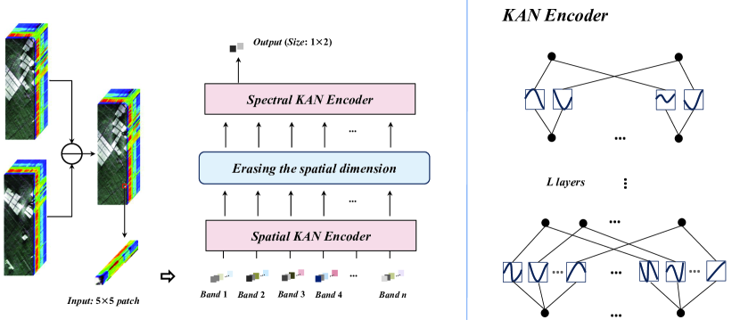
Figure 1: The flowchart of the SpectralKAN. The spectral KAN encoder and the spatial KAN encoder share the same structure, differing only in the number of layers and nodes. The right is the detailed structure of the KAN encoder.

III SpectralKAN

In this section, we first review preliminaries of KAN. Then, the SpectralKAN with two well-designed modules, KAN encoder and spatial-spectral KAN encoder, is introduced. And the flowchart of the SpectralKAN is illustrated in Fig. 1.

III-A A Review of KANs

MLPs are constructed from layers of interconnected nodes (neurons), each with associated weights and activation functions. However, the limitation of MLPs a fixed and uniform activation function for all node can impair their nonlinear fitting capabilities. The computational formula of MLPs can be seen in (1), where $\alpha$ is the activate function, $l\in[1,2,\dots,L]$ is the layer number, and $\mathbf{W}_{l}$ is the weight of layer $l$. KANs address the above problem by introducing heterogeneous activation functions, thereby enhancing the model’s expressive power and adaptability, and providing a more robust tool for fitting complex patterns. KANs can be expressed as (2). $\bf\Phi_{\textit{l}}$ is a function vector that represents the activation functions of the $l$-th layer, with each neuron having a different activation function. Furthermore, KANs overcomes the limitations of the Kolmogorov–Arnold representation theorem, which restricts the number of hidden layers to 2 and the number of nodes in each hidden layer to $2n+1$ (where $n$ is the number of input elements). KANs can have any number of layers, and each layer can have any number of nodes. Assuming the input to the $l$-th layer of KANs is $\mathbf{x}_{l}\in\mathbb{R}^{n_{l}}$ and the output is $\mathbf{x}_{l+1}\in\mathbb{R}^{n_{l+1}}$, the computation formula can be seen in (3).

$$MLP(\mathbf{x})=\mathbf{x}\cdot\prod_{l=0}^{L-1}\mathbf{W}_{l}\alpha$$ (1)

$$KAN(\mathbf{x})=\mathbf{x}\cdot\prod_{l=0}^{L-1}\bf\Phi_{\textit{l}}$$ (2)

$$\begin{split}&\mathbf{x}_{l+1}=\Phi_{\textit{l}}\mathbf{x}_{l},\\ &\Phi_{\textit{l}}(\cdot)=\begin{pmatrix}\phi_{l,1,1}(\cdot)&\phi_{l,1,2}(\cdot)&\dots&\phi_{l,1,n_{l}}(\cdot)\\ \phi_{l,2,1}(\cdot)&\phi_{l,2,2}(\cdot)&\dots&\phi_{l,2,n_{l}}(\cdot)\\ &&\vdots&\\ \phi_{l,n_{l+1},1}(\cdot)&\phi_{l,n_{l+1},2}(\cdot)&\dots&\phi_{l,n_{l+1},n_{l}}(\cdot)\\ \end{pmatrix}\end{split}$$ (3)

Actually, KANs learns the activation functions $\mathbf{\Phi}$, whereas MLPs learn the weights $\mathbf{W}$. How does KANs learn the $\mathbf{\Phi}$? Let’s take a look at what $\phi(\cdot)$ is. The structure is showed in Fig. 2(a). It consists of two activation functions with weight such that

$$\phi(x)=w_{a}\alpha(x)+w_{b}spline(x)$$ (4)

where $\alpha(\cdot)$ usually refers to sigmoid linear unit (SiLU) function. $spline(\cdot)$ is composed of multiple B-spline basis functions:

$$spline(x)=\sum_{i=0}^{s}c_{i}B^{k}_{i}(x)$$ (5)

where $B^{k}_{i}(x)$ is the i-th B-spline basis function, $c_{i}$ is the corresponding weight, $s$ is the number of knot span, decided by knot vector, and $k$ is the degree of $spline(\cdot)$. Each $B^{k}_{i}(x)$ is a piece wise polynomial determined by a knot vector and a degree $k$. By appropriately choosing the knot vector, $k$, and $\mathbf{c}$, the spline function can approximate any continuous function. $w_{a}$ and $w_{b}$ are the weights of $\alpha(\cdot)$ and $spline(\cdot)$, respectively. They are used to control the scaling and amplification of $\alpha(\cdot)$ and $spline(\cdot)$. So, KANs learns the weights $w_{a}$, $w_{b}$ and $\mathbf{c}$ to construct any nonlinear activate function for each $\phi(\cdot)$ by back propagation. In some tasks, KANs with just a few layers can achieve state-of-the-art accuracy while requiring fewer FLOPs, less GPU memory, shorter training and testing time compared to deep MLPs-based networks.

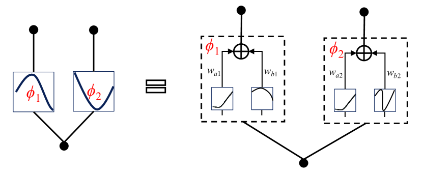
(a)

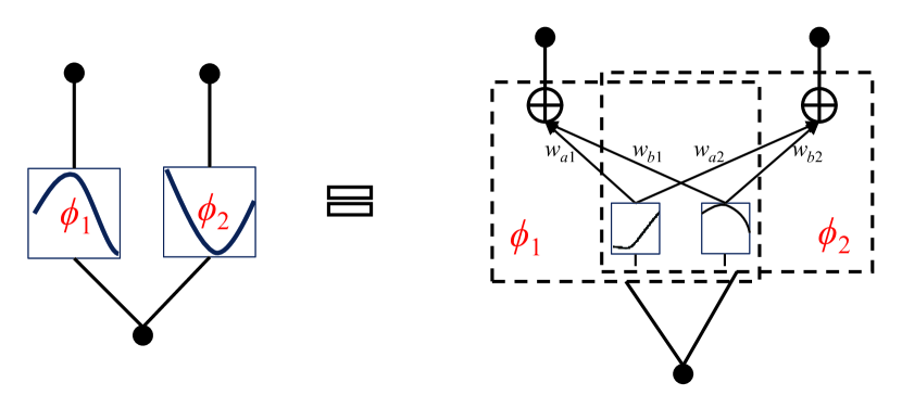
(b)

Figure 2: Using an input of 1 and an output of 2 as an example, the detailed structure diagram of the activation function. Each dashed box represents an activation function $\phi(\cdot)$. (a) KANs. (b) KAN encoder.

III-B KAN encoder

For HSIs, the dimensional of input is very large for KANs. This still faces the problem of a large number of parameters and high FLOPs. So, a KAN encoder is introduced for HSIs feature extraction.

The flowchart of KAN encoder is showed in Fig. 1. It same to the stricture of KANs [5]. Each $\phi(\cdot)$ is composed by $\alpha(\cdot)$ and $spline(\cdot)$ with their weight in both KANs and KAN encoder, as shown in Eq. (4). The main difference is that in KANs, each $\phi(\cdot)$ of each node in each layer has its own $\alpha(\cdot)$ and $spline(\cdot)$, whereas in the KAN encoder, all $\phi(\cdot)$ of each node in each layer share $\alpha(\cdot)$ and $spline(\cdot)$, as shown in Fig. 2.

Let’s look at the benefits of sharing $\alpha(\cdot)$ and $spline(\cdot)$ in the KAN encoder. The main FLOPs of a $\phi(\cdot)$ include the FLOPs of $\alpha(\cdot)$ and $spline(\cdot)$, as well as their respective multiplications by $w_{a}$ and $w_{b}$ in both KANs and KAN encoder. For a single-element input, the FLOPs of $\alpha(\cdot)$ is 4, and the FLOPs of $spline(\cdot)$ is 96. The FLOPs for their respective weight multiplications is 1 each. The main parameters of a $\phi(\cdot)$ include $w_{a}\in\mathbb{R}^{1\times 1}$, $w_{b}\in\mathbb{R}^{1\times 1\times 8}$ and $\textbf{c}\in\mathbb{R}^{1\times 1\times 8}$. For single-layer, the FLOPs of KANs and KAN encoder is $(96+4+1+1)\times dim_{i}\times dim_{o}$ and $(96+4)\times dim_{i}+(1+1)\times dim_{i}\times dim_{o}$, respectively. $dim_{i}$ and $dim_{o}$ are the number of nodes of input and output. The single-layer KAN encoder has $100\times dim_{i}\times(dim_{o}-1)$ fewer FLOPs than the single-layer KANs. The number of parameters of KANs and KAN encoder is $(1+8+8)\times dim_{i}\times dim_{o}$ and $(1+8)\times dim_{i}\times dim_{o}+8\times dim_{i}$. There are $8\times dim_{i}\times(dim_{o}-1)$ parameters that have been reduced. When dealing with high-dimensional HSIs, both $dim_{i}$ and $dim_{o}$ are large. The KAN encoder is more effective in reducing the numbers of FLOPs and parameters. Additionally, the spectral curve of HSIs can be considered as approximately continuous discrete signals. Therefore, there is some redundancy in information between adjacent spectral signals. The KAN encoder that uses a shared $\alpha(\cdot)$ and $spline(\cdot)$ for single spectral signal will not result in information loss compared to KANs.

III-C Spatial-Spectral KAN Encoder

To more effectively extract the features of HSIs, we designed a spatial-spectral KAN encoder to capture the spatial-spectral features of HSIs. While the KAN encoder still has a large number of parameters and FLOPs for high-dimensional HSIs data, the spatial-spectral KAN encoders deal with lower spatial and spectral dimensions separately, significantly reducing the number of parameters and FLOPs.

We assume that there is a pair of co-registered bi-temporal HSIs, denoted as $\mathbf{X_{1}}$ and $\mathbf{X_{2}}$. We can get the difference map $\mathbf{X}=\mathbf{X_{1}}-\mathbf{X_{2}}$. Then, $\mathbf{X}$ is cropped into numerous patches $\mathbf{x}=[x_{1},x_{2},\dots]$, $x\in\mathbb{R}^{p\times p\times b}$ to be used as the input of SpectralKAN. $p\times p$ is the patch size, $b$ is the number of bands in $\mathbf{X}$. We reshape $x$ from $\mathbb{R}^{p\times p\times b}$ into $\mathbb{R}^{b\times p^{2}}$. $x$ is fed into the spatial KAN encoder to get the output $z\in\mathbb{R}^{b\times 1}$

$$z=\mathbf{\Phi}_{1,L_{m}-1}\odot\dots\odot\mathbf{\Phi}_{1,1}\odot\mathbf{\Phi}_{1,0}\odot x$$ (6)

where $\mathbf{\Phi}_{1,l_{m}}$ represents the activate functions of the $l_{m}+1$ layer spatial KAN encoder. There are $L_{m}$ layers in total. The final layer of spatial KAN encoder has only one node that compress the spatial dimension of $x$ patch size to one. Then, we reshape $z$ from $\mathbb{R}^{b\times 1}$ to $\mathbb{R}^{b}$, eliminating the spatial dimension of $z$. In spite of having only spectral dimensions, $z$ still retains spatial feature information. In the end, we input $z$ into the spectral KAN encoder to extract spectral features and obtain the CD result directly from the last layer of spectral KAN encoder.

$$y^{\prime}=\mathbf{\Phi}_{2,L_{n}-1}\odot\dots\odot\mathbf{\Phi}_{2,1}\odot\mathbf{\Phi}_{2,0}\odot z$$ (7)

where $\mathbf{\Phi}_{2,l_{n}}$ represents the activate functions of the $l_{n}+1$ layer spectral KAN encoder. There are $L_{n}$ layers in total. $y^{\prime}\in\mathbb{R}^{2}$ is the output of SpectralKAN. We use the cross-entropy function to calculate the loss between $y$ and $y^{\prime}$ to update the network.

Let’s take a look at how the spatial KAN encoder and spectral KAN encoder reduce the number of parameters and FLOPs. If $x\in\mathbb{R}^{p\times p\times b}$ is input into a two-layer KAN encoder with $q$ nodes in the second layer, the number of parameter is $bp^{2}(9q+8)$. Similarly, if $x$ is separated into spatial and spectral dimensions, and processed using the spatial KAN encoder and spectral KAN encoder respectively, the number of parameters is $(b+p^{2})(9q+8)$. The former has $bp^{2}/(b+p^{2})\approx p^{2}$ times the number of parameters compared to the latter. At the same time, the FLOPs are also reduced by approximately $p^{2}$ times.

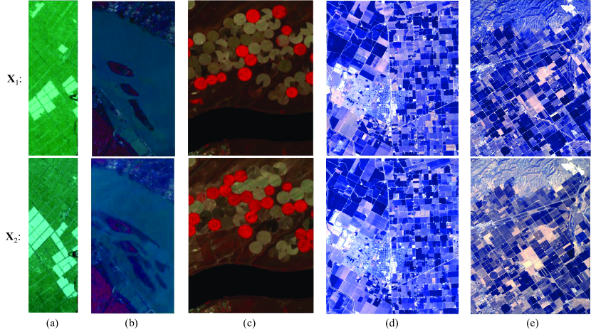
Figure 3: Pseudo-color images of five HSIs-CD datasets. The first row is the before-temporal HSIs, and the second row is the the after-temporal HSIs. (a) Farmland. (b) river. (c) USA. (d) Bay Area. (e) Santa Barbara.

TABLE I: Details of Five HSIs-CD Datasets

Dataset	Satellite Sensor	Image Times	Cover Land	Size $(h\times w\times b)$	Spatial Resolution	Main Change
Farmland	EO-1 Hyperion	05. 2006 and 04. 2007	Yancheng, China	450 $\times$ 140 $\times$ 155	30m	land cover and river
river	EO-1 Hyperion	05. 2013 and 12. 2013	Jiangsu, China	431 $\times$ 241 $\times$ 198	30m	substance in river
USA	EO-1 Hyperion	05. 2004 and 05. 2007	Hermiston, USA	307 $\times$ 241 $\times$ 154	30m	land cover and river
Bay Area	AVIRIS	2013 and 2015	Bay Area, USA	600 $\times$ 500 $\times$ 224	20m	land cover
Santa Barbara	AVIRIS	2013 and 2014	Santa Barbara, USA	984 $\times$ 740 $\times$ 224	20m	land cover

TABLE II: The Number of Training and Test Sets in the Five Datasets, in Units of Pixels (p).

Dataset	Unchanged	Changed	Unknown	Training Set		Testing Set
				Unchanged	Changed	Unchanged	Changed
Farmland	44723	18277	0	447	182	44276	18095
river	101885	9698	0	1018	96	100867	9602
USA	57311	16676	0	573	166	56738	16510
Bay Area	34211	39270	226519	342	392	33869	38878
Santa Barbara	80418	52134	595608	804	521	79614	51613

IV Experiments

This section first introduces the HSIs-CD datasets used in the experiments. Secondly, the experimental environment and the hyperparameters of SpectralKAN are described. Then, we conduct comparative experiments with state-of-the-art methods and ablation analyses to verify the effectiveness of proposed SpectralKAN. Finally, the hyperparameters are analyzed.

IV-A HSIs-CD Datasets

We uses five HSIs-CD datasets, including Farmland, river [41], USA [42], Bay Area, and Santa Barbara datasets, to analyze the advantages and disadvantages of proposed SpectralKAN and the existing commonly used methods. These five datasets were obtained by the Earth Observation-1 Hyperion hyperspectral sensor (EO-1 Hyperion) and the Airborne Visible/Infrared Imaging Spectrometer sensor (AVIRIS). The pseudo-color images are showed in Fig. 3. Detailed information for five datasets is provided in Table I. For each dataset, we use only $1\%$ of the pixels as training sets, with the others used as test sets, as detailed in Table II.

IV-B Experimental Setup

The SpectralKAN was trained using Pytorch = 2.3.0 + cu118, Intel® Core™ i9-10900K CPU and an NVIDIA Corporation TU102 [TITAN RTX] GPU. The operating system is Ubuntu 20.04.1 LTS. The $k$ and grid in B-spline basis function is 3 and 5, respectively. $s$ is obtained by adding $k$ and grid. The numbers of spatial and spectral KAN encoder layer $(l_{m}$ and $l_{n})$ are both 3. The patch size is $5\times 5$. So the note numbers of 3-layer spatial KAN encoder are 25, 16, and 1. The node numbers of the 2-layer spectral KAN encoder are $b$ and 2. The number of training epochs is 200. The batch size is 64. The Adam optimizer is used for gradient descent. The learning rate is 0.001, and it is multiplied by 0.9 every 10 epochs. The parameters ($w_{a}$, $W_{b}$, and c) are initialized using the Kaiming initialization method.

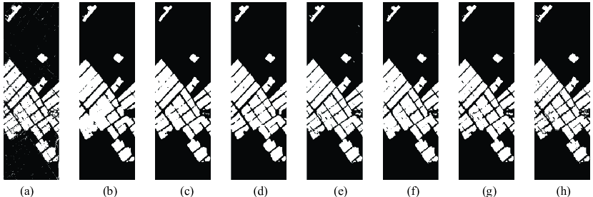
Figure 4: HSIs-CD results on Farmland datasets. (a) CVA. (b) SVM. (c) SST-Former. (d) CSANet. (e) TriTF. (f) DA-Former. (g) SpectralKAN. (h) Ground Truth. The white pixels are changed, and the black pixels are unchanged.

TABLE III: The OA and $\mathcal{K}$ Comparison of State-of-the-art HSI-CD Methods on Farmland.

	OA	$\mathcal{K}$	Parameters($k$)	FLOPs($M$)	Memory($M$)	Training Times($s$)	Testing Times($s$)
CVA	0.9589	0.9003	-	-	-	-	0.39
SVM	0.9600	0.9033	-	-	-	0.001	1.10
SST-Former	0.9743	0.9379	2498	145	1370	56.87	7.52
CSANet	0.9619	0.9075	2428	140	1561	63.9	7.85
TriTF	0.9754	0.9403	172	21	2406	49.02	16.06
DA-Former	0.9657	0.9174	398	30	1586	1444.43	10.46
SpectralKAN	0.9801	0.9514	8	0.07	911	13.26	2.52

Six commonly used state-of-the-art methods, CVA, SVM, SST-Former [13], CSANet [43], TriTF [15], DA-Former [44] are used as comparison methods. Overall accuracy (OA) and Kappa ($\mathcal{K}$) are used for a quantitative analysis of the performance of each methods. At the same time, we also compare the number of parameter, FLOPs, GPU memory usage, and training and testing times among different methods, as these indicators are also important for applications in HSIs-CD. CVA and SVM are machine learning methods, their number of parameters and FLOPs are significantly lower than those of deep learning methods. Moreover, they can run on a general CPU. Therefore, we do not count their number of parameters, FLOPs, and GPU memory. CVA is an unsupervised method, so it has no training time. Except for CVA , all methods are evaluated under the same experimental settings and use the same number of training samples.

IV-C Comparison with State-of-the-art Methods

Fig. 4, 5, 6, 7, 8 show the visual results for the Farmland, river, USA, Bay Area, and Santa Barbara using state-of-the-art methods, respectively. OA, $\mathcal{K}$, the number of parameters, FLOPs, GPU memory, training and testing times for the five datasets are listed in Table. III, IV, V,  VI, and VII, respectively.

1) Results Analysis for the Farmland Dataset: As shown in Fig. 4, there is a significant amount of salt-and-pepper noise in the CVA map. SVM, SST-Former and DA-Former did not perform well on edge. SVM, SST-Former, and CSANet got some missed alarm areas. TriTF’s map had a bit of salt-and-pepper noise. In terms of visual quality, the SpectralKAN performed better. In Table. III, we can see that the CVA and SVM had the top two training and testing times and required minimal computational resources. However, their OA and $\mathcal{K}$ were relatively low. For deep learning-based methods, SpectralKAN had the best OA, $\mathcal{K}$, the number of parameters, FLOPs, GPU Memory, training and testing times. And SpectralKAN far exceeded the second best deep learning methods in terms of the number of parameters, FLOPs, GPU Memory, training and testing times.

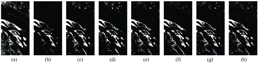
Figure 5: HSIs-CD results on river datasets. (a) CVA. (b) SVM. (c) SST-Former. (d) CSANet. (e) TriTF. (f) DA-Former. (g) SpectralKAN. (h) Ground Truth. The white pixels are changed, and the black pixels are unchanged.

TABLE IV: The OA and $\mathcal{K}$ Comparison of State-of-the-art HSI-CD Methods on river.

	OA	$\mathcal{K}$	Parameters($k$)	FLOPs($M$)	Memory($M$)	Training Times($s$)	Testing Times($s$)
CVA	0.9259	0.6541	-	-	-	-	0.77
SVM	0.9554	0.6557	-	-	-	0.01	0.76
SST-Former	0.9644	0.7671	2520	148	1483	124.15	15.7
CSANet	0.9501	0.6762	2452	144	1586	29.9	10.84
TriTF	0.9699	0.8099	181	22	2486	95.45	31.42
DA-Former	0.9509	0.7041	409	32	1455	1477.47	20.11
SpectralKAN	0.9745	0.8366	9	0.09	961	25.55	5.1

2) Results Analysis for the river Dataset: As depicted in Fig. 5, CVA had the lots of false positives areas, and SVM had the lots of false negatives areas. The edges of small objects were not well detected by SST-Former and CSANet, and there are many missed alarm areas. DA-Former also had many missed alarm in small changed areas. The visual results of TriTF and SpectralKAN were better, with few little false negatives on small objects. Similar to the Farmland, as shown in Table 4, CVA and SVM had the shortest training and testing times and used the least computational resources, but their OA and $\mathcal{K}$ were also the lowest. SpectralKAN had the highest OA and $\mathcal{K}$. Compared to other deep learning methods, SpectralKAN had the lowest number of parameters, FLOPs, GPU memory usage, and training and testing times.

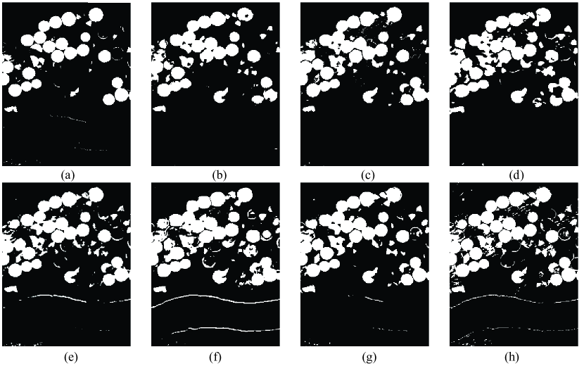
Figure 6: HSIs-CD results on USA datasets. (a) CVA. (b) SVM. (c) SST-Former. (d) CSANet. (e) TriTF. (f) DA-Former. (g) SpectralKAN. (h) Ground Truth. The white pixels are changed, and the black pixels are unchanged.

TABLE V: The OA and $\mathcal{K}$ Comparison of State-of-the-art HSI-CD Methods on USA.

	OA	$\mathcal{K}$	Parameters($k$)	FLOPs($M$)	Memory($M$)	Training Times($s$)	Testing Times($s$)
CVA	0.9200	0.7408	-	-	-	-	0.46
SVM	0.9325	0.7879	-	-	-	0.01	1.6
SST-Former	0.9431	0.8286	2498	145	1373	65.67	8.82
CSANet	0.9374	0.8167	2427	140	1561	77.5	9.73
TriTF	0.9563	0.8701	171	21	2418	59.69	19.89
DA-Former	0.9348	0.8169	398	30	1970	1269.04	12.41
SpectralKAN	0.9591	0.8804	8	0.07	911	15.8	2.89

3) Results Analysis for the USA Dataset: We can see that all HSIs-CD results in Fig. 6 exhibit varying degrees of missed alarm areas. The visual results of CVA, SVM, SST-Former and CSANet were all subpar. TriTF, DA-Former, and SpectralKAN performed well in large objects but struggle in narrow and small objects. From the quality analysis results in Table V, CVA and SVM had the top two inference times and resource efficiency but rank the lowest in OA and $\mathcal{K}$. Compared to CVA and SVM, deep learning methods achieve significantly higher accuracy, but this comes with a large number of parameters, increased FLOPs, GPU memory usage, and inference times. SpectralKAN achieved the highest accuracy and also significantly reduced parameters, FLOPs, and other resource demands compared to existing deep learning methods.

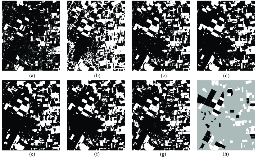
Figure 7: HSIs-CD results on Bay Area datasets. (a) CVA. (b) SVM. (c) SST-Former. (d) CSANet. (e) TriTF. (f) DA-Former. (g) SpectralKAN. (h) Ground Truth. The white pixels are changed, and the black pixels are unchanged. The gray pixels are unknown on ground truth.

TABLE VI: The OA and $\mathcal{K}$ Comparison of State-of-the-art HSI-CD Methods on Bay Area.

	OA	$\mathcal{K}$	Parameters($k$)	FLOPs($M$)	Memory($M$)	Training Times($s$)	Testing Times($s$)
CVA	0.8517	0.7063	-	-	-	-	2.28
SVM	0.8994	0.7973	-	-	-	0.01	2.80
SST-Former	0.9661	0.932	2534	150	1581	78.89	52.71
CSANet	0.9826	0.9652	2468	147	1564	48.1	31.01
TriTF	0.9814	0.9626	186	22	2496	64.88	102.64
DA-Former	0.9807	0.9612	416	33	1991	1309.59	56.65
SpectralKAN	0.9641	0.9329	10	0.1	981	17.33	14.18

4) Results Analysis for the Bay Area Dataset: From a visual (Fig. 7) of view, the result of SVM was confusing. The CD map of CVA performed best in edge details. However, it also had a significant amount of missed and false alarm areas. Deep learning methods had all good detection effects in labeled areas. At the same time, SpectralKAN provided the second best edge detail. From a quantity (Table. VI) of view, the $\mathcal{K}$ of CVA and SVM were 10%-20% lower than those of deep learning methods. CSANet, TriTF, and DA-Former had the first, second, and third best OA and $\mathcal{K}$, respectively. However, they require more computing resources and longer inference time. Although SpectralKAN was 3.05% lower than CSANet, it showed a qualitative improvement in parameters, FLOPs, GPU memory, training and testing times.

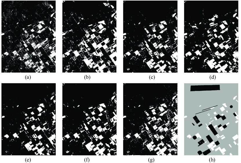
Figure 8: HSIs-CD results on Santa Barbara datasets. (a) CVA. (b) SVM. (c) SST-Former. (d) CSANet. (e) TriTF. (f) DA-Former. (g) SpectralKAN. (h) Ground Truth. The white pixels are changed, and the black pixels are unchanged. The gray pixels are unknown on ground truth.

TABLE VII: The OA and $\mathcal{K}$ Comparison of State-of-the-art HSI-CD Methods on Santa Barbara.

	OA	$\mathcal{K}$	Parameters($k$)	FLOPs($M$)	Memory($M$)	Training Times($s$)	Testing Times($s$)
CVA	0.8325	0.6519	-	-	-	-	6.09
SVM	0.9634	0.9344	-	-	-	0.02	4.00
SST-Former	0.9752	0.9478	2534	150	1544	149.85	134.62
CSANet	0.9916	0.9823	2468	147	1368	144.2	75.25
TriTF	0.9854	0.9693	186	22	2464	134.07	250.28
DA-Former	0.992	0.9832	416	33	1984	1590.66	140.03
SpectralKAN	0.9776	0.9531	10	0.1	981	30.10	34.72

5) Results Analysis for the Santa Barbara Dataset: From Fig. 8, we can observe that CVA and SVM exhibited a lot of salt-and-pepper noise. All deep learning methods perform well and similarly in the annotated regions. In Table. VII, the OA and $\mathcal{K}$ of CVA was the worst. SVM was approximately 28% higher than CVA in $\mathcal{K}$. The deep learning-based methods outperformed SVM by approximately 1% to 5%. DA-Former was the best OA and $\mathcal{K}$. However, its training time is very long. The SpectralKAN showed a 2.67% decrease in OA compared to DA-Former. But its computational efficiency is the best in deep learning methods.

In conclusion, CVA had the shortest test time and took up the least computing resources, but it also had the lowest accuracy and often generated a lot of salt and pepper noise. And each pixel occupies a large area, for example, a spatial pixel represent $30m\times 30m$ areas in the Farmland dataset, so the impact of salt and pepper noise cannot be ignored. SVM had very low computing resource usage and short inference time, but its accuracy is far lower than that of deep learning methods. For deep learning methods, SST-Former had the largest number of parameters and FLOPs. While its accuracy is not the highest across the five datasets, it remained stable. CSANet exhibited instability, performing excellently on the Bay Area and Santa Barbara datasets but poorly on the other three datasets. TriTF achieved high accuracy across all five datasets, but it also had the highest GPU memory usage. DA-Former had an extremely long training time. SpectralKAN achieved the best OA and $\mathcal{K}$ on the Farmland, River, and USA datasets, its accuracy on the other two datasets was not lacking. In addition, SpectralKAN significantly outperformed other deep learning methods in parameters, FLOPs, GPU memory, and training and testing times.

IV-D Ablation Experiments

Ablation experiments were conducted to validate the effectiveness of KANs, as well as the KAN encoder and Spatial-Spectral KAN encoder proposed in this paper. Table. VIII show the results on five datasets. We previously analyzed the reasons for the reduction in parameters and FLOPs of KAN encoder and Spatial-Spectral KAN encoder. GPU memory usage, training and testing times are related to parameters and FLOPs, so, we only selected the number of parameters and $\mathcal{K}$ as evaluation metrics in Table. VIII. We abbreviated the Spatial-Spectral encoder as SS in Table. VIII. Firstly, we compared the a MLP and a KAN, both with 16 hidden layer nodes, and found that the $\mathcal{K}$ of KAN is significantly higher than that of MLP. However, it is worth noting that the number of parameter in KAN is ten times that of MLP. A similar conclusion can be drawn between MLP+SS and KAN+SS. Secondly, we discovered that applying the KAN encoder can reduce the parameter number by approximately four times, as evidenced by comparing KAN and KAN+KAN encoder, as well as comparing KAN+SS and KAN+SS+KAN encoder (SpectralKAN). Additionally, with the reduction in number of parameter, the $\mathcal{K}$ of methods incorporating the KAN encoder increased on several datasets and decreased on others, with both increases and decreases being minimal. Then, three comparison experiments, MLP and MLP+SS, KAN and KAN+SS, KAN+KAN encoder and SpectralKAN, demonstrated that the spatial-spectral structure reduced the number of parameter by more than 20 times while improving $\mathcal{K}$, indicating that the spatial-spectral KAN encoder can more effectively enhance the spatial-spectral features of HSIs. Finally, considering both parameters and $\mathcal{K}$, we conclude that KAN+KAN encoder+SS (SpectralKAN) is the best. Additionally, we found that MLP+SS is a good choice when accuracy is not overly emphasized.

TABLE VIII: The $\mathcal{K}$ and Number of Parameters in the Ablation Experiment For KAN, KAN Encoder and Spatial-Spectral Structure. Bold indicates the best. Blue indicates the second best.

	KAN encoder	SS	Farmland		river		USA		Bay Area		Barbara
			$\mathcal{K}$	Params($k$)	$\mathcal{K}$	Params($k$)	$\mathcal{K}$	Params($k$)	$\mathcal{K}$	Params($k$)	$\mathcal{K}$	Params($k$)
MLP	✗	✗	0.8842	62	0.5516	79	0.8106	62	0.5269	89	0.8859	89
	✗	✓	0.9262	3	0.6189	4	0.8473	3	0.8683	4	0.9363	4
KAN	✗	✗	0.9435	620	0.7638	792	0.8437	616	0.9109	896	0.9479	896
	✓	✗	0.9426	155	0.7648	198	0.8423	154	0.9185	224	0.9529	224
	✗	✓	0.9497	29	0.8219	36	0.878	29	0.9347	40	0.9565	40
	✓	✓	0.9514	8	0.8366	9	0.8804	8	0.9329	10	0.9531	10

IV-E Effect of Hyperparameters

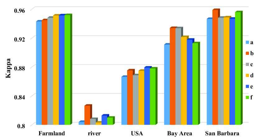
Figure 9: The $\mathcal{K}$ of different nodes and layers on five datasets.

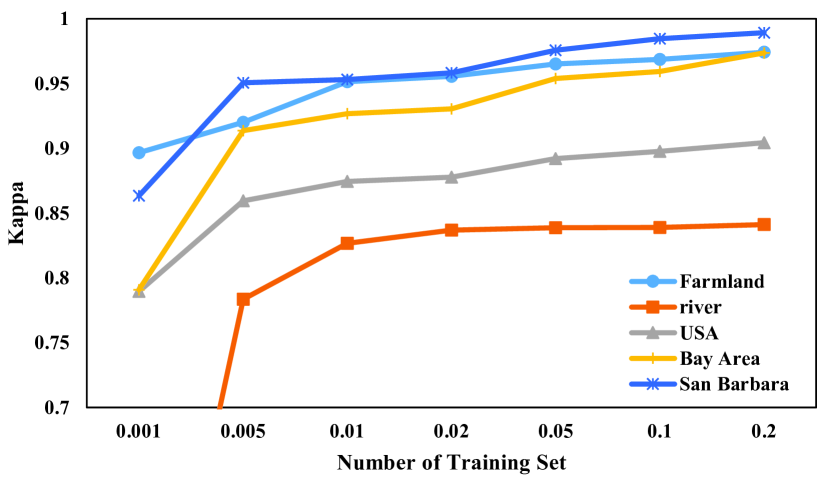
Figure 10: The $\mathcal{K}$ of different training set number on five datasets.

Different numbers of nodes and hidden layers in SpectralKAN will result in different parameter number and accuracy. We selected six different combinations of nodes and layers to identify the optimal parameters: a: [25,1], [b,2], b: [25, 16, 1], [b, 2], c: [25, 1], [b, 16, 2], d: [25, 16, 1], [b, 16, 2], e: [25, 64, 1], [b, 16, 2], and f: [25, 16, 1], [b, 64, 2]. In a-f, the first set represents the number of nodes in the spatial KAN encoder, and the second set represents the number of nodes in the spectral KAN encoder. From a to f, the number of nodes or layers gradually increases, accompanied by an increase in parameter number. The $\mathcal{K}$ of experiments can be seen in Fig. 9. In the Farmland dataset, as the number of nodes or layers increases, the $\mathcal{K}$ also gradually increases. In the other datasets, however, no consistent pattern is observed. Considering both number of parameters and Kappa, we determine that b is the best configuration.

Different tasks have varying requirements for number of training set. 0.1%, 0.5%, 1%, 2%, 5%, 10%, 20% of the pixels as training sets to analyze their impact on SpectralKAN. The results are shown in Fig. 10. We observe that with a larger number of training set, the accuracy of CD increases.

V Conclusion

In this paper, we explore the application of KAN for HSIs-CD for the first time, and propose a specialized approach called SpectralKAN tailored to the task. The parameter-reducing KAN encoder does not diminish the accuracy of HSIs-CD. The spatial-spectral KAN encoder not only significantly reduces the number of parameter but also effectively enhances the extraction of spatial-spectral features from HSIs. Through extensive experiments, we validated that SpectralKAN achieves state-of-the-art accuracy while significantly reducing parameters, FLOPs, GPU memory usage, training, and testing times. SpectralKAN can be integrated into more compact devices, making it more practical for scenarios such as emergency missions. Nevertheless, the testing time of SpectralKAN still lags behind that of machine learning methods like SVM, making it a point for further research.

References

- [1] F. Bovolo, S. Marchesi, and L. Bruzzone, “A framework for automatic and unsupervised detection of multiple changes in multitemporal images,” IEEE Transactions on Geoscience and Remote Sensing, vol. 50, no. 6, pp. 2196–2212, 2011.
- [2] C. Kwan, “Methods and challenges using multispectral and hyperspectral images for practical change detection applications,” Information, vol. 10, no. 11, p. 353, 2019.
- [3] G. Cybenko, “Approximation by superpositions of a sigmoidal function,” Mathematics of control, signals and systems, vol. 2, no. 4, pp. 303–314, 1989.
- [4] K. Hornik, M. Stinchcombe, and H. White, “Multilayer feedforward networks are universal approximators,” Neural networks, vol. 2, no. 5, pp. 359–366, 1989.
- [5] Z. Liu, Y. Wang, S. Vaidya, F. Ruehle, J. Halverson, M. Soljačić, T. Y. Hou, and M. Tegmark, “Kan: Kolmogorov-arnold networks,” arXiv preprint arXiv:2404.19756, 2024.
- [6] T. Zhan, B. Song, L. Sun, X. Jia, M. Wan, G. Yang, and Z. Wu, “Tdssc: A three-directions spectral–spatial convolution neural network for hyperspectral image change detection,” IEEE Journal of Selected Topics in Applied Earth Observations and Remote Sensing, vol. 14, pp. 377–388, 2020.
- [7] A. Song, J. Choi, Y. Han, and Y. Kim, “Change detection in hyperspectral images using recurrent 3d fully convolutional networks,” Remote Sensing, vol. 10, no. 11, p. 1827, 2018.
- [8] M. Gong, F. Jiang, A. K. Qin, T. Liu, T. Zhan, D. Lu, H. Zheng, and M. Zhang, “A spectral and spatial attention network for change detection in hyperspectral images,” IEEE Transactions on Geoscience and Remote Sensing, vol. 60, pp. 1–14, 2021.
- [9] L. Wang, L. Wang, Q. Wang, and P. M. Atkinson, “Ssa-siamnet: Spectral–spatial-wise attention-based siamese network for hyperspectral image change detection,” IEEE Transactions on Geoscience and Remote Sensing, vol. 60, pp. 1–18, 2021.
- [10] Y. Yang, J. Qu, S. Xiao, W. Dong, Y. Li, and Q. Du, “A deep multiscale pyramid network enhanced with spatial–spectral residual attention for hyperspectral image change detection,” IEEE Transactions on Geoscience and Remote Sensing, vol. 60, pp. 1–13, 2022.
- [11] M. Hu, C. Wu, and L. Zhang, “Globalmind: Global multi-head interactive self-attention network for hyperspectral change detection,” ISPRS Journal of Photogrammetry and Remote Sensing, vol. 211, pp. 465–483, 2024.
- [12] H. Yu, H. Yang, L. Gao, J. Hu, A. Plaza, and B. Zhang, “Hyperspectral image change detection based on gated spectral–spatial–temporal attention network with spectral similarity filtering,” IEEE Transactions on Geoscience and Remote Sensing, 2024.
- [13] Y. Wang, D. Hong, J. Sha, L. Gao, L. Liu, Y. Zhang, and X. Rong, “Spectral–spatial–temporal transformers for hyperspectral image change detection,” IEEE Transactions on Geoscience and Remote Sensing, vol. 60, pp. 1–14, 2022.
- [14] W. Dong, Y. Yang, J. Qu, S. Xiao, and Y. Li, “Local information enhanced graph-transformer for hyperspectral image change detection with limited training samples,” IEEE Transactions on Geoscience and Remote Sensing, 2023.
- [15] X. Wang, K. Zhao, X. Zhao, and S. Li, “Tritf: A triplet transformer framework based on parents and brother attention for hyperspectral image change detection,” IEEE Transactions on Geoscience and Remote Sensing, vol. 61, pp. 1–13, 2023.
- [16] S. Liu, H. Li, F. Wang, J. Chen, G. Zhang, L. Song, and B. Hu, “Unsupervised transformer boundary autoencoder network for hyperspectral image change detection,” Remote Sensing, vol. 15, no. 7, p. 1868, 2023.
- [17] X. Zhang, S. Tian, G. Wang, X. Tang, J. Feng, and L. Jiao, “Cast: A cascade spectral aware transformer for hyperspectral image change detection,” IEEE Transactions on Geoscience and Remote Sensing, 2023.
- [18] M. Han, J. Sha, Y. Wang, and X. Wang, “Pbformer: Point and bi-spatiotemporal transformer for pointwise change detection of 3d urban point clouds,” Remote Sensing, vol. 15, no. 9, p. 2314, 2023.
- [19] Q. Guo, J. Zhang, C. Zhong, and Y. Zhang, “Change detection for hyperspectral images via convolutional sparse analysis and temporal spectral unmixing,” IEEE Journal of Selected Topics in Applied Earth Observations and Remote Sensing, vol. 14, pp. 4417–4426, 2021.
- [20] X. Ou, L. Liu, B. Tu, G. Zhang, and Z. Xu, “A cnn framework with slow-fast band selection and feature fusion grouping for hyperspectral image change detection,” IEEE Transactions on Geoscience and Remote Sensing, vol. 60, pp. 1–16, 2022.
- [21] J. Qu, Y. Xu, W. Dong, Y. Li, and Q. Du, “Dual-branch difference amplification graph convolutional network for hyperspectral image change detection,” IEEE Transactions on Geoscience and Remote Sensing, vol. 60, pp. 1–12, 2021.
- [22] J. Qu, J. Zhao, W. Dong, S. Xiao, Y. Li, and Q. Du, “Feature mutual representation based graph domain adaptive network for unsupervised hyperspectral change detection,” IEEE Transactions on Geoscience and Remote Sensing, 2023.
- [23] W. Zhang, Y. Zhang, S. Gao, X. Lu, Y. Tang, and S. Liu, “Spectrum-induced transformer based feature learning for multiple change detection in hyperspectral images,” IEEE Transactions on Geoscience and Remote Sensing, 2023.
- [24] F. Luo, T. Zhou, J. Liu, T. Guo, X. Gong, and J. Ren, “Multiscale diff-changed feature fusion network for hyperspectral image change detection,” IEEE Transactions on Geoscience and Remote Sensing, vol. 61, pp. 1–13, 2023.
- [25] J. Qu, W. Dong, Y. Yang, T. Zhang, Y. Li, and Q. Du, “Cycle-refined multidecision joint alignment network for unsupervised domain adaptive hyperspectral change detection,” IEEE Transactions on Neural Networks and Learning Systems, 2024.
- [26] B. Bai, W. Fu, T. Lu, and S. Li, “Edge-guided recurrent convolutional neural network for multitemporal remote sensing image building change detection,” IEEE Transactions on Geoscience and Remote Sensing, vol. 60, pp. 1–13, 2021.
- [27] C. Shi, Z. Zhang, W. Zhang, C. Zhang, and Q. Xu, “Learning multiscale temporal–spatial–spectral features via a multipath convolutional lstm neural network for change detection with hyperspectral images,” IEEE Transactions on Geoscience and Remote Sensing, vol. 60, pp. 1–16, 2022.
- [28] W. Dong, J. Zhao, J. Qu, S. Xiao, N. Li, S. Hou, and Y. Li, “Abundance matrix correlation analysis network based on hierarchical multihead self-cross-hybrid attention for hyperspectral change detection,” IEEE Transactions on Geoscience and Remote Sensing, vol. 61, pp. 1–13, 2023.
- [29] D. A. Sprecher and S. Draghici, “Space-filling curves and kolmogorov superposition-based neural networks,” Neural Networks, vol. 15, no. 1, pp. 57–67, 2002.
- [30] P.-E. Leni, Y. D. Fougerolle, and F. Truchetet, “The kolmogorov spline network for image processing,” in Image Processing: Concepts, Methodologies, Tools, and Applications. IGI Global, 2013, pp. 54–78.
- [31] C. J. Vaca-Rubio, L. Blanco, R. Pereira, and M. Caus, “Kolmogorov-arnold networks (kans) for time series analysis,” arXiv preprint arXiv:2405.08790, 2024.
- [32] R. Genet and H. Inzirillo, “Tkan: Temporal kolmogorov-arnold networks,” arXiv preprint arXiv:2405.07344, 2024.
- [33] K. Xu, L. Chen, and S. Wang, “Kolmogorov-arnold networks for time series: Bridging predictive power and interpretability,” arXiv preprint arXiv:2406.02496, 2024.
- [34] Z. Huang, J. Cui, L. Yu, L. F. Herbozo Contreras, and O. Kavehei, “Abnormality detection in time-series bio-signals using kolmogorov-arnold networks for resource-constrained devices,” medRxiv, pp. 2024–06, 2024.
- [35] M. Liu, S. Bian, B. Zhou, and P. Lukowicz, “ikan: Global incremental learning with kan for human activity recognition across heterogeneous datasets,” arXiv preprint arXiv:2406.01646, 2024.
- [36] Z. Bozorgasl and H. Chen, “Wav-kan: Wavelet kolmogorov-arnold networks,” arXiv preprint arXiv:2405.12832, 2024.
- [37] D. W. Abueidda, P. Pantidis, and M. E. Mobasher, “Deepokan: Deep operator network based on kolmogorov arnold networks for mechanics problems,” arXiv preprint arXiv:2405.19143, 2024.
- [38] J. Xu, Z. Chen, J. Li, S. Yang, W. Wang, X. Hu, and E. C.-H. Ngai, “Fourierkan-gcf: Fourier kolmogorov-arnold network–an effective and efficient feature transformation for graph collaborative filtering,” arXiv preprint arXiv:2406.01034, 2024.
- [39] M. Cheon, “Kolmogorov-arnold network for satellite image classification in remote sensing,” arXiv preprint arXiv:2406.00600, 2024.
- [40] A. Jamali, S. K. Roy, D. Hong, B. Lu, and P. Ghamisi, “How to learn more? exploring kolmogorov-arnold networks for hyperspectral image classification,” arXiv preprint arXiv:2406.15719, 2024.
- [41] Q. Wang, Z. Yuan, Q. Du, and X. Li, “Getnet: A general end-to-end 2-d cnn framework for hyperspectral image change detection,” IEEE Transactions on Geoscience and Remote Sensing, vol. 57, no. 1, pp. 3–13, 2018.
- [42] M. Hasanlou and S. T. Seydi, “Hyperspectral change detection: An experimental comparative study,” International journal of remote sensing, vol. 39, no. 20, pp. 7029–7083, 2018.
- [43] R. Song, W. Ni, W. Cheng, and X. Wang, “Csanet: Cross-temporal interaction symmetric attention network for hyperspectral image change detection,” IEEE Geoscience and Remote Sensing Letters, vol. 19, pp. 1–5, 2022.
- [44] Y. Wang, J. Sha, L. Gao, Y. Zhang, X. Rong, and C. Zhang, “A semi-supervised domain alignment transformer for hyperspectral images change detection,” IEEE Transactions on Geoscience and Remote Sensing, 2023.