MUSE-Net: Missingness-aware mUlti-branching Self-attention Encoder for Irregular Longitudinal Electronic Health Records

Abstract

The era of big data has made vast amounts of clinical data readily available, particularly in the form of electronic health records (EHRs), which provides unprecedented opportunities for developing data-driven diagnostic tools to enhance clinical decision making. However, the application of EHRs in data-driven modeling faces challenges such as irregularly spaced multi-variate time series, issues of incompleteness, and data imbalance. Realizing the full data potential of EHRs hinges on the development of advanced analytical models. In this paper, we propose a novel $\mathbf{M}$issingness-aware m$\mathbf{U}$lti-branching $\mathbf{S}$elf-Attention $\mathbf{E}$ncoder (MUSE-Net) to cope with the challenges in modeling longitudinal EHRs for data-driven disease prediction. The MUSE-Net leverages a multi-task Gaussian process (MGP) with missing value masks for data imputation, a multi-branching architecture to address the data imbalance problem, and a time-aware self-attention encoder to account for the irregularly spaced time interval in longitudinal EHRs. We evaluate the proposed MUSE-Net using both synthetic and real-world datasets. Experimental results show that our MUSE-Net outperforms existing methods that are widely used to investigate longitudinal signals.

Index Terms: Irregularly spaced time series, Multivariate longitudinal records, Data imputation, Imbalanced dataset, Multi-task Gaussian process, Self-attention encoder

1 Introduction

Rapid advancements in sensing and information technology have ushered us into an era of data explosion where a large amount of data is now easily available and accessible in the clinical environment [1, 2, 3]. The wealth of healthcare data offers new avenues for developing data-driven methods for automated disease diagnosis. For instance, there have been growing research interests in harnessing electronic health records (EHRs) to create data-driven solutions for clinical decision support [4] in detecting heart disease [5], sepsis [6], and diabetes [7]. EHRs serve as digital repositories of a patient’s medical information including demographics, medications, vital signs, and lab results [8, 9, 10], curated over time by healthcare providers, leading to a longitudinal database. With rich information about a patient’s health trajectory, longitudinal EHRs present unique opportunities to analyze and decipher clinical events and patterns within large populations through data-driven machine learning.

However, data mining of longitudinal EHRs poses distinctive research challenges due to the observational nature of EHRs. Unlike well-defined, randomized longitudinal experiments in clinical trials that collect data on a fixed schedule and ensure high data quality, EHRs are recorded only when patients receive care or doctors provide services. The information collected and the timing of its collection are not determined by researchers, resulting in EHR data that are often complex and highly heterogeneous [11]. Specifically, fully utilizing real-world EHRs for reliable data-driven decision-making calls upon addressing several challenges:

(1) Irregularly spaced time series. EHR data are often documented during irregular patient visits, leading to non-uniform time intervals between successive measurements and a lack of synchronization across various medical variables or among different patients. Traditional time series models face challenges when applied to irregular longitudinal data because they typically assume a parametric form of the temporal variables, making them difficult to effectively account for highly heterogeneous and irregular time intervals across different variables. Additionally, the widely used deep learning models such as convolution neural networks (CNNs) and recurrent neural networks (RNNs) for mining sequential or time series data are designed by assuming consecutive data points are collected at a uniform time interval. Those deep learning models do not consider the elapsed time between records and are less effective in modeling irregular longitudinal EHRs.

(2) Incomplete datasets and imbalanced class distributions. Real-world EHRs suffer from the issues of missing values and imbalanced data. Due to the nature of clinical practice, not all information is recorded for every patient visit, leading to incomplete datasets. Additionally, EHR data often exhibit a significantly imbalanced distribution, with certain health outcomes or characteristics being underrepresented compared to more common ones. For instance, rare diseases or adverse drug reactions [12, 13] may have very few instances compared to more prevalent conditions. In the existing literature, a wide array of statistical and machine learning techniques have been designed to tackle the missing value and imbalanced data issues [14, 15], which, however, are less applicable in the context of modeling irregular longitudinal EHRs. The presence of missing values and imbalanced class distributions will introduce further difficulties in effective model training using longitudinal EHRs, leading to biased or inaccurate predictions if not properly addressed.

To address the multifaceted challenges presented by real-world longitudinal EHRs, this paper introduces a novel framework of $\mathbf{M}$issingness-aware m$\mathbf{U}$lti-branching $\mathbf{S}$elf-Attention $\mathbf{E}$ncoder (MUSE-Net) for data-driven disease prediction. First, multi-task Gaussian processes (MGPs) are employed for missing value imputation in irregularly sampled time series. Second, we propose to add missing value masks that record the locations of missing observations as another input stream to our predictive model, which enables the learning of correlations between non-missing and missing values for mitigating the impact of possible imputation errors incurred from the imputation procedure on the prediction performance. Finally, we propose to integrate a time-aware self-attention encoder with a multi-branching classifier to address the imbalanced data issue and further classify the irregular longitudinal EHRs for disease prediction. We evaluate our proposed framework using both simulation data and real-world EHRs. Experimental results show that our proposed method significantly outperforms existing approaches that are widely used in current practice.

2 Research Background

The integration of data-driven modeling methodologies and EHR data has transformed the healthcare field, which provides unprecedented opportunities for clinical decision support [8, 16, 17]. Extensive research has been conducted to develop data-driven models for disease identification using non-longitudinal EHRs that consist of static or cross-sectional patient health information [18, 19]. For example, Huang et al. [20] employed naive Bayes, decision tree, and nearest neighbor algorithms incorporating feature selection methods to determine key factors affecting type II diabetes control and further identify individuals who exhibit suboptimal diabetes control status. Hong et al. [21] developed a multi-class classification method to analyze clinical data in identifying patients with obesity and various comorbidities using logistic regression, support vector machine, and decision tree algorithms. A comprehensive review on machine learning of non-longitudinal EHRs can be referred to [11, 22]. However, those traditional methods are limited in capturing temporal patterns in patient health status over time. This limitation can result in less accurate predictions for conditions that are heavily dependent on longitudinal health trajectories [18, 23]. Moreover, traditional machine learning approaches often require manual feature engineering, which is not only time-consuming and prone to error but also demands significant domain expertise.

With the growing availability of longitudinal EHRs, increasing interests have been devoted to developing advanced data-driven models to capture critical temporal information for disease prediction. Owing to the outstanding performance and strong capability in pattern recognition, deep learning has been widely explored to mine complexly structured data leveraging the nonlinear interactions among neurons within and across various hidden layers [24, 25, 26, 5]. Advanced network architectures have been crafted for modeling time series or sequential data. For example, recurrent neural networks (RNNs) including long short-term memory (LSTM) are among the most commonly used deep learning models to analyze medical time series for various clinical tasks [27, 28, 29]. Additionally, temporal convolutional networks (TCNs) have been recognized as a robust alternative to RNNs for modeling longitudinal clinical signals [7, 6]. The unique architecture of dilated and causal 1-D convolution and residual blocks [30] allows TCNs to access a broader range of sequential information for capturing long-term temporal dependencies, thereby outperforming RNNs in various tasks involving mining temporal data [7, 6, 31]. However, most existing RNNs and TCNs are designed with the assumption that the longitudinal records are collected at a constant rate and require the neighboring samples to appear at fixed distances to facilitate the convolution or recurrent operations. This assumption is not valid in many real-world databases, making traditional RNNs or TCNs less effective in modeling irregular-spaced longitudinal EHRs.

To cope with the issue of irregular time intervals, many modified RNN architectures have been developed. For example, the time-aware LSTM (TLSTM) was designed to account for non-uniform sampling intervals through a time decay mechanism [32]. Che et al. [28] also implemented a decay mechanism and proposed a GRU-D model for time series signals, allowing the network to better capture temporal dependencies even when data points were incomplete or irregularly sampled. A comprehensive review of modified RNN architectures for irregular sampled time series can be found in [33, 34]. However, most existing time-aware RNNs assume that the impact of historical risk factors on disease prediction proportionally decays over time, which may not be true in describing complex disease trajectories. Additionally, RNNs have been widely recognized as computationally inefficient for modeling large-scale, long sequential data due to their sequential processing nature.

The self-attention encoder, a cornerstone of the transformer architecture [35], has revolutionized the field of natural language processing (NLP) with its unique advantages. Unlike RNNs and TCNs that process data sequentially and require uniform sampling intervals, the self-attention mechanism allows the model to weigh the importance of different parts of the input sequences relative to each other. This feature enables parallel processing and enhances the model’s ability to capture long-range dependencies in irregularly spaced longitudinal signals. For instance, Li et al. proposed to transform time series data into images and adopted the Vision Transformer to model irregularly sampled time series signals [36]. Tipirneni and Reddy developed a method that integrated a continuous value embedding technique with the self-attention architecture to model irregularly sampled clinical time series by treating them as a set of observation triplets (consisting of time, variable, and value)[37]. Huang et al. developed a Deformable Neighborhood Attention Transformer (DNA-T) to capture local and global dependencies in medical time series data through deformable attention mechanisms[38]. Those self-attention-based models demonstrate significant improvements over traditional methods, particularly in handling the irregularities inherent in real-world longitudinal datasets. Despite the strengths of self-attention encoders/transformer architecture, it is worth noting that most standard deep learning algorithms are designed under the assumption that data is ideal, which cannot be directly applied to mine longitudinal EHR databases with missing values and imbalanced class distributions. Little has been done to design an effective framework to model real-world longitudinal EHRs by accounting for the issues of missing values, imbalanced data distribution, and irregular time intervals for robust decision-making.

3 Research Methodology

Suppose that there are $N$ patients indexed by $p\in\{1,\ldots,N\}$ and we denote the dataset as $\mathcal{D}=\{(\boldsymbol{t}_{p},Y_{p},l_{p})\}_{p=1}^{N}$. Each patient is associated with longitudinal data described by the tuple $(\boldsymbol{t}_{p},Y_{p},l_{p})$: $\boldsymbol{t}_{p}=[t_{p,1},t_{p,2},\cdots,t_{p,T_{p}}]$ is the time index set for patient $p$; $Y_{p}=[\boldsymbol{y}_{p,1},\boldsymbol{y}_{p,2},\cdots,\boldsymbol{y}_{p,M}]\in\mathbb{R}^{T_{p}\times M}$ represents the values of $M$ medical variables at $\boldsymbol{t}_{p}$; $l_{p}$ is the binary label with $l_{p}=1$ indicating patient $p$ is positive (e.g., with disease) and otherwise $l_{p}=0$. The length of the time series for each patient is highly variable (i.e., $T_{p}\neq T_{p^{{}^{\prime}}},~{}\text{if}~{}p\neq p^{{}^{\prime}}$ ), and the times series are often irregularly spaced (i.e., $t_{p,i+1}-t_{p,i}\neq t_{p,j+1}-t_{p,j},~{}\text{if}~{}j\neq i$) in real-world longitudinal EHR databases. Additionally, the EHR dataset is often incomplete, and we denote the complete set of values of the $M$ variables as $\boldsymbol{y}_{p}=\text{Vect}(Y_{p})=[\boldsymbol{y}_{p,1}^{T},\boldsymbol{y}_{p,2}^{T},\cdots,\boldsymbol{y}_{p,M}^{T}]^{T}\in\mathbb{R}^{T_{p}M}$. Then, we define an index set that contains observed values as $I_{o}=\{(t,m)|\text{ if }[Y_{p}]_{t,m}\text{ is observed}\}$ and the corresponding values are denoted by $\boldsymbol{y}_{p}^{o}\in\mathbb{R}^{O_{p}}$. Similarly, we define $I_{u}=\{(t,m)|\text{ if }[Y_{p}]_{t,m}\text{ is missing}\}$ as the index set of missing values, and the missing value vector is denoted by $\boldsymbol{y}_{p}^{u}\in\mathbb{R}^{U_{p}}$, where $U_{p}+O_{p}=T_{p}M$. Fig. 1 shows the flowchart of the proposed MUSE-Net to classify irregularly spaced and incomplete longitudinal data. Each component in the flowchart is described in detail in the following subsections.

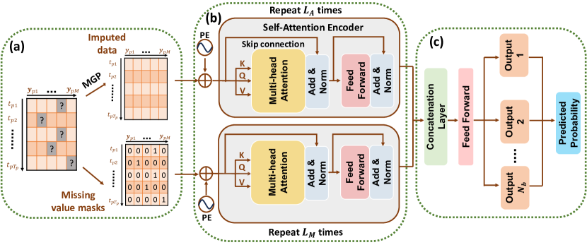
Figure 1: The proposed MUSE-Net framework: (a) Multi-task Gaussian process for data imputation, and missing value masks generation; The imputed data and missing value masks are processed by the proposed MUSE-Net, which consist of (b) Missingness-aware Self-attention Encoder and (c) Multi-branching output layer.

3.1 Multi-task Gaussian Process (MGP) for Missing Value Imputation

A Gaussian process (GP) is a flexible non-parametric Bayesian model where any collection of random variables follows a joint Gaussian distribution [39, 40, 41], which have been widely used to model complex time series data [42, 43]. GP-based temporal models provide a way to determine the distribution of a variable at any arbitrary point in time, making them intrinsically capable of dealing with missing value imputations that involve irregularly spaced longitudinal data. Note that single-task GPs are limited in their ability to model correlations across multiple related tasks (i.e., different medical variables), making them less effective for modeling multi-variate EHR data. To account for the multi-variate nature, we adopt a multi-task GP (MGP) [44], which is an extension to single-task GPs, to capture both variable interactions and temporal correlations for imputing missing values in irregular multi-variate longitudinal EHRs.

We denote $f_{pm}(t)$ as a latent function representing the true values of variable $m$ for patient $p$ at time $t$, and a patient-independent MGP prior is placed over the latent function $f_{pm}(t)$ with a zero mean and the covariance function as:

$$\text{cov}(f_{pm}(t),f_{pm^{{}^{\prime}}}(t^{{}^{\prime}})) = \mathcal{K}_{M}(m,m^{{}^{\prime}})\mathcal{K}_{t}(t,t^{{}^{\prime}})$$

$$y_{pm}(t) \sim \mathcal{N}(f_{pm}(t),\sigma^{2}_{m})$$ (1)

where $y_{pm}(t)$ is the observed value of variable $m$ for patient $p$ at time $t$, $\sigma^{2}_{m}$ is the noise term for the $m$th task (variable), $\mathcal{K}_{M}(m,m^{{}^{\prime}})$ captures the similarities between tasks, and $\mathcal{K}_{t}(t,t^{{}^{\prime}})$ is a temporal correlation function. Note that a fundamental property of time series data is that observations at neighboring points tend to be similar. As such, we use the squared exponential kernel function $\mathcal{K}_{t}(t,t^{{}^{\prime}})=\text{exp}(-\frac{(t-t^{{}^{\prime}})^{2}}{2\theta^{2}})$ with a lengthscale parameter $\theta$. Hence, the prior distribution for the fully observed multivariate longitudinal records, $\boldsymbol{y}^{o}_{p}$, can be represented by:

$$\boldsymbol{y}_{p}^{o}\sim\mathcal{N}(\boldsymbol{0},\Sigma_{p}^{o}),~{}~{}~{}~{}\Sigma_{p}^{o}=\mathcal{K}_{M}\odot\mathcal{K}_{O_{p}}+E$$ (2)

We formulate the kernel function $\Sigma_{p}^{o}$ for the observed records as the combination of the Hadamard product (i.e., element-wise multiplication) of $\mathcal{K}_{M}$ and $\mathcal{K}_{O_{p}}$, and a noise term $E$: $\mathcal{K}_{M}$ is a $O_{p}\times O_{p}$ positive semi-definite covariance matrix over medical variables, which is parameterized by a low-rank matrix $B$ as $LBB^{T}L^{T}$ where $B\in\mathbb{R}^{M\times q}$, and $L\in\mathbb{R}^{O_{p}\times M}$ is an indicator matrix with $L_{im}=1$ if the $i^{\text{th}}$ observation belongs to task $m$ and $\sum_{m=1}^{M}L_{im}=1$; $\mathcal{K}_{O_{p}}$ is a $O_{p}\times O_{p}$ squared exponential correlation matrix over time with elements defined as $\mathcal{K}_{O_{p}}((m,t),(m^{\prime},t^{\prime}))=\mathcal{K}_{t}(t,t^{{}^{\prime}})$ if $(m,t)\in I_{o}$ and $(m^{\prime},t^{\prime})\in I_{o}$; $E$ is a noise matrix with $L\boldsymbol{\sigma}^{2}$ on its main diagonal ($\boldsymbol{\sigma}^{2}\ \in\mathbb{R}^{M}$ and $[\boldsymbol{\sigma}^{2}]_{m}=\sigma_{m}^{2}$ ).

In the inference step, we impute the missing value for patient $p$ using the posterior mean, $\mu_{\boldsymbol{y}_{p}^{u}}$:

$$\mu_{\boldsymbol{y}_{p}^{u}} = (\mathcal{K}_{M_{*}M}\odot\mathcal{K}_{U_{p}O_{p}})(\Sigma_{p}^{o})^{-1}\boldsymbol{y}_{p}^{o}$$ (3)

where $\mathcal{K}_{M_{*}M}=L_{*}BB^{T}L^{T}\in\mathbb{R}^{U_{p}\times O_{p}}$ is the task covariance matrix for missing values, and $L_{*}\in\mathbb{R}^{U_{p}\times M},L_{*,im}=1$ if the $i^{\text{th}}$ missing value belongs to task $m$; $\mathcal{K}_{U_{p}O_{p}}$ represents the correlation matrix between the time points of the observed and missing values. The hyperparameters in the MGP model include the lower triangular matrix $B$, error term $\text{Diag}(E)$, and the lengthscale $\theta$ in $\mathcal{K}_{O_{p}}$: $\boldsymbol{\Theta}=\{\text{Vect}(B),\text{Diag}(E),\theta\}$, which are learned by minimizing the negative log marginal likelihood given by (with derivative)

$$\mathcal{L}(\boldsymbol{\Theta}) = \log|\Sigma_{p}^{o}|+(\boldsymbol{y}_{p}^{o})^{T}(\Sigma_{p}^{o})^{-1}\boldsymbol{y}_{p}^{o}+\frac{O_{p}}{2}\log(2\pi)$$

$$\frac{d\mathcal{L}}{d\boldsymbol{\Theta}} = (\boldsymbol{y}_{p}^{o})^{T}(\Sigma_{p}^{o})^{-1}\frac{d\Sigma_{p}^{o}}{d\boldsymbol{\Theta}}(\Sigma_{p}^{o})^{-1}\boldsymbol{y}_{p}^{o}+\text{Tr}\left((\Sigma_{p}^{o})^{-1}\frac{d\Sigma_{p}^{o}}{d\boldsymbol{\Theta}}\right)$$ (4)

Finally, the missing values in $Y_{p}$ are estimated as $\hat{\boldsymbol{y}}_{p}^{u}=\mu_{\boldsymbol{y}_{p}^{u}}$, which are combined with the observed values $\boldsymbol{y}_{p}^{o}$ to form an imputed dataset $\hat{\mathcal{D}}=\{(\boldsymbol{t}_{p},\hat{Y}_{p},l_{p})\}_{p=1}^{N}=\{((\boldsymbol{t}_{p}^{o},\text{Vect}^{-1}(\boldsymbol{y}_{p}^{o})),(\boldsymbol{t}_{p}^{u},\text{Vect}^{-1}(\hat{\boldsymbol{y}}_{p}^{u})),l_{p})\}_{p=1}^{N}$, where $\text{Vect}^{-1}(\cdot)$ is the inverse operation of $\text{Vect}(\cdot)$.

In addition, to accelerate MGP Imputation, we adopt the black box matrix-matrix multiplication framework [45] to integrate the modified preconditioned conjugate gradient (mPCG) approach with GPU acceleration into the data imputation workflow. Please refer to Appendix 8.3 for the detailed procedure for GPU acceleration of MGP imputation.

3.2 Missingness-aware Multi-branching Self-Attention Encoder (MUSE-Net)

We further propose a novel missingness-aware multi-branching self-attention encoder network (MUSE-Net) to process the imputed longitudinal EHRs. This model is designed to not only effectively capture crucial temporal correlations in multi-variate irregular longitudinal data but also recognize missingness patterns and account for the imbalanced data issue for enhanced classification performance. As shown in Fig. 1(b) and (c), this model consists of 3 key modules: time-aware self-attention encoder, missing value masks, and multi-branching outputs.

3.2.1 Time-aware Self-attention Encoder

We propose to adapt the traditional self-attention encoder [35] to incorporate the information of elapsed time between consecutive records in irregular longitudinal EHRs. Specifically, there are three building blocks in our time-aware self-attention encoder:

Elapsed time-based positional encoding: The time order of the input longitudinal sequence plays a crucial role in time series analysis. However, this information is often ignored in traditional attention-based encoders because it does not incorporate any recurrent or convolution operations. To address this issue, an elapsed time-based positional encoding is added into the input sequence at the beginning of the self-attention encoder as shown in Fig. 1(b), such that the temporal information regarding the irregularly sampled EHRs is incorporated into the model. In our study, we employ the following sinusoidal encoding:

$$PE_{t_{p,i},2m}=\text{sin}(t_{p,i}/10000^{2m/M})\quad\quad\quad PE_{t_{p,i},2m+1}=\text{cos}(t_{p,i}/10000^{2m/M})$$ (5)

where $t_{p,i}$ is the time position of each observation to account for the irregularly spaced time interval, and $2m$ and $2m+1$ represent the ($2m$)-th and ($2m+1$)-th variable dimensions, respectively. The sinusoid prevents positional encodings from becoming too large, introducing extra difficulties in network optimization. The embedded elapsed time-based positional features will then be combined with the imputed longitudinal sequence to generate the input of the self-attention module: $X_{p}=PE_{p}+\hat{Y}_{p}$, where $PE_{p}\in\mathbb{R}^{T_{p}\times M}$ is a matrix with elements defined in Eq. (5).

Self-attention module: The self-attention module is the fundamental mechanism that allows the network to learn dependencies in the longitudinal data. It maps a query set and a set of key-value pairs to an output. In a typical single-head self-attention, the key, query, and value matrices, denoted as $K\in\mathbb{R}^{T_{p}\times M}$, $Q\in\mathbb{R}^{T_{p}\times M}$, and $V\in\mathbb{R}^{T_{p}\times M}$, are computed by taking the input $X_{p}$:

$$K=\mathcal{F}_{K}(X_{p}),~{}~{}Q=\mathcal{F}_{Q}(X_{p}),~{}~{}V=\mathcal{F}_{V}(X_{p})$$ (6)

where $\mathcal{F}_{K}(\cdot)$, $\mathcal{F}_{Q}(\cdot)$, and $\mathcal{F}_{V}(\cdot)$ represent the network operations to calculate the key, query, and value matrices respectively, which are often selected as linear transformations. The corresponding output, $\text{Output}_{S}\in\mathbb{R}^{T_{p}\times M}$, is computed by applying the scaled-dot production attention:

$$\text{Output}_{S}=\text{softmax}(\frac{QK^{T}}{\sqrt{M}})\times V$$ (7)

where $\text{softmax}(\boldsymbol{x})_{i}=\frac{e^{x_{i}}}{\sum_{j}e^{x_{j}}}$ outputs the weight assigned to each element in $V$. Note that the dot product in the softmax function is scaled down by $\sqrt{M}$. This is essential to prevent the dot product values from growing too large, especially when the dimensionality of $\hat{Y}_{p}$ or $X_{p}$ is large, introducing instabilities in the training process. The self-attention mechanism enables the network to access all the information of the input with the flexibility of focusing on certain important elements over the entire sequence, unlike the RNNs or CNNs which focus more on the neighboring elements.

The multi-head attention module is an extension of single-head self-attention to capture different relations among multivariate time series, which is adopted in our study to model complex longitudinal EHRs. Specifically, we define multiple matrices for the keys, queries, and values by applying multiple network operations, $\mathcal{F}_{K}^{l}(\cdot)$’s, $\mathcal{F}_{Q}^{l}(\cdot)$’s, and $\mathcal{F}_{V}^{l}(\cdot)$’s, to the input:

$$K_{l}=\mathcal{F}_{K}^{l}(X_{p})\in\mathbb{R}^{T_{p}\times\frac{M}{h}},~{}~{}Q_{l}=\mathcal{F}_{Q}^{l}(X_{p})\in\mathbb{R}^{T_{p}\times\frac{M}{h}},~{}~{}V_{l}=\mathcal{F}_{V}^{l}(X_{p})\in\mathbb{R}^{T_{p}\times\frac{M}{h}}$$ (8)

where $h$ is the number of attention heads and $l\in\{1,\dots,h\}$. The output of each attention head, $\text{Output}_{l}\in\mathbb{R}^{T_{p}\times\frac{M}{h}}$, is calculated by:

$$\text{Output}_{l}=\text{softmax}(\frac{Q_{l}K_{l}^{T}}{\sqrt{M/h}})\times V_{l}$$ (9)

The final output of the multi-head attention, $\text{Output}_{M}\in\mathbb{R}^{T_{p}\times M}$, is the multiplication of the concatenation of the outputs of all heads and a weight matrix, $W^{O}\in\mathbb{R}^{M\times M}$:

$$\text{Output}_{M}=[\text{Output}_{1},\text{Output}_{2},\cdots,\text{Output}_{h}]W^{O}$$ (10)

This multi-head attention module enables the network to jointly attend to information from different subspaces of multivariate time series at different time points. Simple visualization of the computing procedure of multi-head attention can be found in Fig. 2.

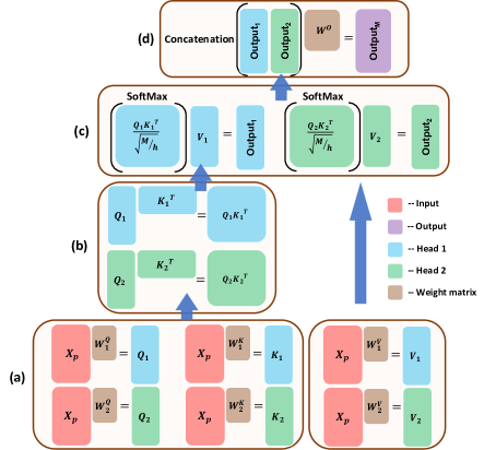
Figure 2: Illustration of multi-head attention with 2 heads. (a) Derivation of $Q,K,V$ matrices for each head with linear transformations of $X_{p}$: $Q_{l}=\mathcal{F}_{Q}^{l}(X_{p})=X_{p}W_{l}^{Q}$, $K_{l}=\mathcal{F}_{K}^{l}(X_{p})=X_{p}W_{l}^{K}$, $V_{l}=\mathcal{F}_{V}^{l}(X_{p})=X_{p}W_{l}^{V}$, $l=\{1,2\}$; (b) Compute key-query pairs for each head; (c) Compute attention weights from softmax function and further compute the output of heads 1 and 2 as the weighted sum of values; (d) The final output is the multiplication of the concatenation of all head outputs and another weight matrix $W^{O}$.

Feed-forward network: To stabilize the training process, $\text{Output}_{M}$ will pass through a layer normalization operation [46], and the normalized output will be combined with the original input using skip-connection [47] to generate the output of the “Add & Norm” block (see Fig. 1(b)):

$$\text{Output}_{AN}=\text{LayerNorm}(\text{Output}_{M})+X_{p}$$ (11)

$\text{Output}_{AN}$ will serve as the input of a feed-forward network with GELU [48] activation and additional “Add & Norm” blocks to further induce nonlinearity degree into the self-attention encoder. The multi-head attention and feed-forward modules will be repeated multiple times to improve the generalizability of the model for capturing more informative features of the input sequence.

3.2.2 Missing Value Masks

To further account for potential discrepancies between imputed values and actual observations, the missing value masks (see Fig. 1(a)) are incorporated as an additional input to the proposed model. We define the missing value masks for patient $p$ as $\tilde{X}_{p}$ with $[\tilde{X}_{p}]_{t,m}=1$ if $[Y_{p}]_{t,m}$ is missing; otherwise $[\tilde{X}_{p}]_{t,m}=0$. The masks will be processed by an independent time-aware self-attention encoder in parallel with the imputed sequences as shown in Fig. 1(b). This missingness-aware design enables the network to capture the relationship between non-missing and missing values. As a result, the network is capable of mitigating the effect of potential imputation errors during the MGP imputation process, thereby enhancing the overall predictive performance of the model.

3.2.3 Multi-branching Outputs

The self-attention encoder serves as a powerful feature extractor from irregular longitudinal EHRs for downstream tasks, such as binary classification. The classifier network, typically with a fully connected layer, is added after the feature extractor to interpret the abstracted features and make a final classification of the original input. The imbalanced data issue, a common problem in healthcare databases, incurs a more pronounced and direct negative impact on the classifier than on the feature extractor network. This is due to the fact that the classifier network directly interacts with the labels and is heavily influenced by the majority class during the training process [49]. This leads to a bias towards the majority class, visibly affecting the model’s performance. As such, careful design of the classifier network is needed to cope with the imbalanced data issue.

We propose to incorporate the Multi-branching (MB) architecture [6] (see Fig.1 (c)) into the classifier network to tackle the imbalanced issue. Specifically, in the training phase, the self-attention encoder will be trained with the whole dataset, and each of the MB outputs in the classifier network will be trained with a balanced sub-dataset to mitigate the negative influence of imbalanced data. The original imputed dataset $\hat{\mathcal{D}}$ consists of the majority class $\hat{\mathcal{D}}_{M}$, and the minority class $\hat{\mathcal{D}}_{N}$. We create $N_{b}$ balanced sub-datasets by under-sampling $\hat{\mathcal{D}}_{M}$ to form $\mathcal{D}_{i}=\{\hat{\mathcal{D}}_{N},\hat{\mathcal{D}}_{M}^{i}\}$, where the $\hat{\mathcal{D}}_{M}=\hat{\mathcal{D}}_{M}^{1}\cup\hat{\mathcal{D}}_{M}^{2}\cup\cdots\cup\hat{\mathcal{D}}_{M}^{N_{b}}$. This under-sampling operation is also applied to the missing value masks. Correspondingly, $N_{b}$ output branches are created, each aligned with one of the balanced sub-datasets. Thus, each balanced sub-dataset serves as the training data for the respective branch in the output layer, and the self-attention encoder will be optimized by using all the $N_{b}$ balanced subsets. In the end, the MB output layer will produce $N_{b}$ predicted probabilities. The optimization process is guided by minimizing the cross-entropy loss function:

$$\mathcal{L}(\boldsymbol{\omega};\hat{\mathcal{D}})=-\sum_{p=1}^{N}\sum_{i=1}^{N_{b}}I(p\in\mathcal{D}_{i})\left(l_{p}\log(\hat{P}^{(i)}(\hat{Y}_{p},\tilde{X}_{p};\boldsymbol{\omega}))+(1-l_{p})\log(1-\hat{P}^{(i)}(\hat{Y}_{p},\tilde{X}_{p};\boldsymbol{\omega}))\right)$$ (12)

where $\boldsymbol{\omega}$ denotes the network parameters from both the self-attention encoder and the MB classifier; $I(\cdot)$ is an indicator function; $\hat{P}^{(i)}(\hat{Y}_{p},\tilde{X}_{p};\boldsymbol{\omega})$ is the predicted probability by output branch $i$ given the input data $\hat{Y}_{p}$ and corresponding missing value mask $\tilde{X}_{p}$. The final predicted probability for patient $p$ is computed as the average of the $N_{b}$ predicted probabilities: $\hat{P}_{MB}(\hat{Y}_{p},\tilde{X}_{p};\boldsymbol{\omega})=\sum_{i=1}^{N_{b}}\hat{P}^{(i)}(\hat{Y}_{p},\tilde{X}_{p};\boldsymbol{\omega})/N_{b}$, which is a more robust estimator compared to the single-branch (SB) counterpart as stated in Theorem I.

Theorem I: If both MB and SB classifiers are sufficiently trained with the following assumptions:

$$\bar{\hat{P}}^{(i)}(Y_{p}) = \bar{\hat{P}}_{SB}(Y_{p}),~{}~{}~{}~{}~{}~{}~{}~{}~{}(i\in\{1,\dots,N_{b}\})$$

$$\mathbb{E}_{\boldsymbol{\omega}}[D_{KL}(\bar{\hat{P}}^{(i)}(Y_{p})||\hat{P}^{(i)}(Y_{p};\boldsymbol{\omega}))] = \mathbb{E}_{\boldsymbol{\omega}}[D_{KL}(\bar{\hat{P}}_{SB}(Y_{p})||\hat{P}_{SB}(Y_{p};\boldsymbol{\omega}))],$$ (13)

where $\hat{P}_{SB}(Y_{p};\boldsymbol{\omega})$ is the predicted distribution by the SB classifier for input $Y_{p}$, $D_{KL}(\cdot)$ is the Kullback–Leibler divergence, $\bar{\hat{P}}_{SB}(Y_{p})=\arg\min_{P_{*}}\mathbb{E}_{\boldsymbol{\omega}}[D_{KL}(P_{*}(Y_{p})||\hat{P}_{SB}(Y_{p};\boldsymbol{\omega}))]$, and $\bar{\hat{P}}^{(i)}(Y_{p})=\arg\min_{P_{*}}\mathbb{E}_{\boldsymbol{\omega}}[D_{KL}(P_{*}(Y_{p})||\hat{P}^{(i)}(Y_{p};\boldsymbol{\omega}))]$, then the variance of the MB classifier is no larger than the variance of the SB classifier, i.e., $V_{MB}\leq V_{SB}$, where

$$V_{MB} = \mathbb{E}_{Y_{p}\sim P_{data},\boldsymbol{w}}[D_{KL}(\bar{\hat{P}}_{MB}(Y_{p})||\hat{P}_{MB}(Y_{p};\boldsymbol{w}))]$$ (14)

$$V_{SB} = \mathbb{E}_{Y_{p}\sim P_{data},\boldsymbol{w}}[D_{KL}(\bar{\hat{P}}_{SB}(Y_{p})||\hat{P}_{SB}(Y_{p};\boldsymbol{w}))]$$ (15)

Here, $P_{data}$ denotes the true data distribution and

$$\bar{\hat{P}}_{MB}(Y_{p}) = \arg\min_{P_{*}}\mathbb{E}_{\boldsymbol{\omega}}[D_{KL}(P_{*}(Y_{p})||\hat{P}_{MB}(Y_{p};\boldsymbol{\omega}))]$$ (16)

Theorem I shows that the MB classifier is more robust than the SB classifier (see Appendix 8.2 for the theoretical proof).

Figure 3: Illustration of the experimental design to evaluate the performance of the proposed MUSE-Net.

4 Experimental Design and Results

Fig. 3 shows our experimental design to evaluate the performance of the proposed MUSE-Net. We implement our MUSE-Net to investigate both a synthetic and real-world dataset for performance evaluation. The MUSE-Net is benchmarked with four popular model structures widely used in sequential modeling: LSTM [50], gated recurrent unit (GRU) [51], Time-aware LSTM (T-LSTM) [32], and TCN [30]. Additionally, we evaluate the prediction performance provided by different imputation methods, i.e., the proposed MGP+mask, MGP, single Gaussian process (GP), GP+mask, the baseline mean imputation, and Mean+mask. We also evaluate the impact of the number of branches on the final prediction performance. The dataset in both synthetic and real-world case studies is split into training (80%), validation (10%), and testing (10%) sets to facilitate a comprehensive training and evaluation process. The model performance is evaluated based on two key metrics: area under the receiver operating characteristic curve (AUROC) and area under the precision-recall curve (AUPRC). AUROC serves as a measure of the model’s ability to discriminate between classes, with a value of 1.0 indicating perfect classification and 0.5 denoting no discriminative power. AUPRC is especially valuable for assessing performance in classifying imbalanced datasets, reflecting the balance between precision and recall across various thresholds.

Algorithm 1 Synthetic Data Generation Process

1:Number of time steps: $n\_obs=200$; Number of observations sampled from each time series: $sub\_time=50$; Number of variables: $n\_variables=10$; Number of samples to generate: $n\_samples=5000$; Percentage of the majority samples: $percent\_negative=90\%$

2:Initialize $\Omega_{m}$ for ARMA($p_{m}$,$q_{m}$), $m\in\{1,2,3\}$, and apply feature engineering to generate remaining ARMA($p_{m}$,$q_{m}$) $m\in\{4,5,\cdots,2\times n\_variables\}$

3:Generate a label list, $labels\_list$, including $n\_samples$ binary labels (0 or 1) based on $percent\_negative$

4:Generate empty 3-D tensor, $all\_samples$, to store the generated data

5:for $j\leftarrow 1$ to $n\_samples$ do

6:    Initialize an empty temporal list: $variables\leftarrow[\quad]$

7:    for $m\leftarrow 1$ to $n\_variables$ do

8:         if $label\_list[j]$ is $0$ (negative instance) then $\triangleright$ For negative instance

9:             Generate $n\_variables$ time series data using $\text{ARMA}(p_{m},q_{m})$

10:         else$\triangleright$ For positive instance

11:             Generate $n\_variables$ time series data using $\text{ARMA}(p_{m+n\_variables},q_{m+n\_variables})$          

12:         Add generated time series to $variables$     

13:    Combine $variables$ into a matrix with $n\_variables$ columns and add it to $all\_samples$

14:Initialize an empty tensor: $final\_dataset$

15:for $i\leftarrow 1$ to $n\_samples$ do

16:    $subtime\_indices\leftarrow$ Maintains the temporal order and randomly selects $sub\_time$ unique time steps

17:    $sub\_ts\_i\leftarrow all\_samples$[$i$, $subtime\_indices$, :]

18:    Add generated $sub\_ts\_i$ to $final\_dataset$

19:return $final\_dataset$

4.1 Experimental Results in Synthetic Case Study

Algorithm 1 shows the process to generate synthetic data from the autoregressive moving average (ARMA) model [52]. Specifically, we first generate three baseline time series variables by ARMA($p_{m}$,$q_{m}$) models with moving average of order $q_{m}$ and autoregressive of order $p_{m}$: $v_{m,t}=\phi_{m,1}v_{m,t-1}+\cdots+\phi_{m,p_{m}}v_{m,t-p_{m}}+\psi_{m,1}\epsilon_{m,t-1}+\cdots+\psi_{m,q_{m}}\epsilon_{m,t-q_{m}}+\epsilon_{m,t}$, where $\{\epsilon_{m,t}\}$ are uncorrelated random variables for variable $m$; $\Omega_{m}=\{\phi_{m,1},\cdots,\phi_{m,p_{m}},\psi_{m,1},\cdots,\psi_{m,q_{m}}\}$ is the set of coefficients for variable $m$. We initialize $\Omega_{m}$ randomly from a standard normal distribution and randomly select $p_{m}$,$q_{m}$ from set $\{1,2,3\}$. We generate the remaining seven variables through feature engineering applied to the three baseline time series, ensuring correlations exist among the variables and differences exist between different classes. Detailed information on the feature engineering process and the simulation parameters is available in the Appendix 8.1. The generated synthetic dataset is a 3-D tensor containing 5,000 samples with 90% from the majority class. Each sample has 10 variables measured across 50 time steps with irregular intervals. Notably, each variable is characterized by a distinct rate of missing values, varying randomly between 30% and 60%, mimicking real-world data complexities.

Fig. 4 shows the AUROC and AUPRC scores over training epochs for the MUSE-Net-9 (i.e., with 9 branching outputs) utilizing different imputation methods with missing value masks on the validation set of our simulated data. The ‘complete’ represents the scenario where MUSE-Net is trained on synthetic data without any missing values. The MUSE-Net-9+MGP method exhibits superior performance in both AUROC/AUPRC metrics and convergence speed. In contrast, the MUSE-Net-9+GP and MUSE-Net-9+mean methods display delayed convergence and lower scores, especially in the AUPRC metric.

Fig. 5 displays the AUROC and AUPRC scores across training epochs for MUSE-Net+MGP with different numbers of MB outputs on the simulated validation set. It is evident that within 8 epochs, all the MUSE-Nets achieve optimal performance, reaching near-perfect AUROC and AUPRC scores. This exceptional performance is partly due to the simplistic nature of the synthetic dataset and the high efficacy of MGP imputation and effective feature extraction achieved by the MUSE-Net. However, we observe variations in the convergence speed among different MB numbers. Specifically, as we increase the MB outputs from 1 to 9, the speed of convergence improves. This enhancement can be attributed to the improved balance in the training sub-dataset for each branching output. With only one output, the imbalanced ratio is as skewed as 9:1, presenting a significant challenge for the model to learn from the minority class. As the number of MB outputs increases to 9, the ratio between the positive and negative classes is approximately 1:1, providing a more balanced learning environment for each branch. As such, the network model can learn more effectively from both classes, leading to faster convergence.

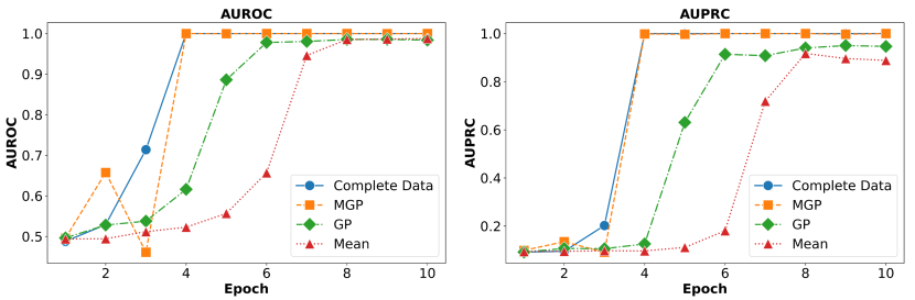
Figure 4: AUROC and AUPRC scores across epochs for MUSE-Net-9 utilizing different imputation methods on the validation set of the simulated data.

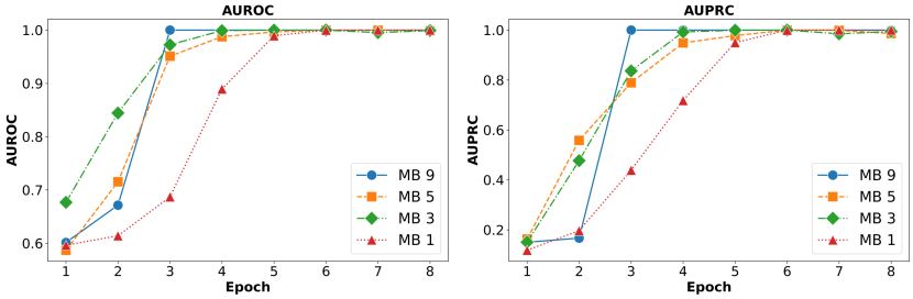
Figure 5: AUROC and AUPRC scores across epochs for MUSE-Net with different numbers of MB outputs on the validation set of the simulated data imputed by MGP.

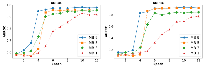
Figure 6: AUROC and AUPRC scores across epochs for MUSE-Net with mean imputation and different numbers of MB outputs on the validation set of the simulated data.

The impact of imbalanced data is more significant when modeling datasets with poor quality. Fig. 6 shows the AUROC and AUPRC scores across epochs for MUSE-Net with mean imputation and different numbers of MB outputs on the synthetic validation set. The mean imputation is known for introducing a high bias due to its simplistic assumption, resulting in a less reliable imputed dataset. According to Fig. 6, the MUSE-Net-9 converges within 6 epochs and achieves a good AUROC/AUPRC score, which indicates that our MB architecture together with the missing value masks effectively mitigates the negative impact of imbalanced datasets, even when the imputed training data is with low quality. In contrast, the MUSE-Net does not converge in 12 epochs if the MB architecture is not incorporated (i.e., MB 1) and the final AUROC/AUPRC scores decrease to 0.921/0.773 from 0.988/0.895.

4.2 Experimental Results in Real-world Case Study

We further conduct a real-world case study using the Diabetic Retinopathy (DR) dataset, obtained from the 2018 Cerner Health Facts data warehouse [7, 29], to evaluate our MUSE-Net. The medical variables selected for this study include 21 routine blood tests, 5 comorbidity indicators, 3 demographic variables, and the duration of diabetes. More details on variable selection can be referred to [29, 53]. Notably, the 21 blood tests are all subject to missing values, and the final dataset consists of records from 23,245 diabetic patients, with a minority of 8.9% diagnosed with DR. We use label “1” and “0” to indicate that a patient diagnosed with and without DR, respectively.

Fig. 7 shows the performance of our MUSE-Net compared to other benchmark models on the DR validation set. Note that to ensure a fair comparison, all models are designed to have similar sizes, with the number of model parameters approximately 4,300, as shown in Table 1. Furthermore, all models utilize the MGP imputation with missing value masks, 10 MB outputs, and Adam with decoupled weight decay optimizer [54]. According to Fig. 7, our MUSE-Net consistently outperforms other benchmarks, achieving the highest AUROC and AUPRC scores on the validation set. This trend is also evident in the results for the test set summarized in Table LABEL:tab:Model_scores_test, where MUSE-Net maintains the AUROC score of 0.949 and the AUPRC score of 0.883, which dominates those yielded by TCN, LSTM, T-LSTM, and GRU models. Specifically, the MUSE-Net has an improvement over TCN by 2.3% in AUROC and 5.3% in AUPRC, and an improvement over LSTM by 3.3% in AUROC and 7.1% in AUPRC, an improvement over T-LSTM by 2.4% in AUROC and 6.8%, and an improvement over GRU 1.9% in AUROC and 4.6% in AUPRC. This performance demonstrates that MUSE-Net is more effective at capturing the critical patterns inherent in irregular longitudinal DR data. The higher AUROC and AUPRC scores reflect the superior performance of our MUSE-Net in terms of both discrimination and precision-recall balance, which are critical for clinical decision making.

Table 1: Architectures of MUSE-Net and other benchmarks for DR dataset.

	Number of model parameters	Number of layers (blocks)	Number of outputs in MB layer	Optimizer
MUSE-Net	4,282	2	10	Adam with decoupled weight decay (AdamW) [54]
GRU	4,333
LSTM	4,686
T-LSTM	4,525
TCN	4,396

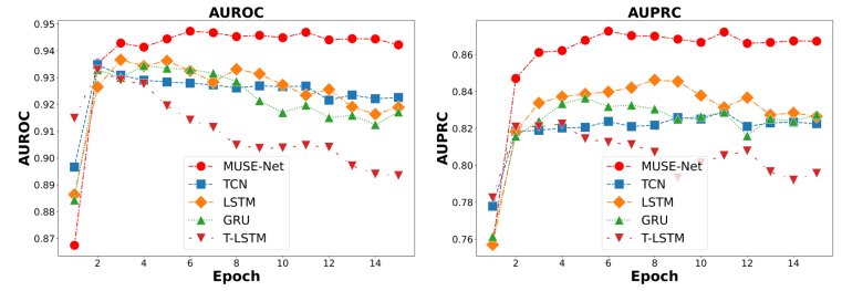
Figure 7: AUROC and AUPRC across 15 epochs for our MUSE-Net and other benchmarks on the DR validation set.

Table 2: AUROC and AUPRC scores for MUSE-Net and other benchmarks on the DR test set.

	MUSE-Net	TCN	LSTM	T-LSTM	GRU
AUROC	0.949	0.928	0.919	0.927	0.932
AUPRC	0.883	0.839	0.825	0.827	0.844

Table 3 presents the performance comparison in AUROC and AUPRC between our MUSE-Net-10 with MGP imputation and other imputation methods on the DR test set. It is worth noting that the MUSE-Net-10 with MGP+masks outperforms other methods, yielding an AUROC of 0.949 and an AUPRC of 0.883, which represents an improvement over GP+masks by 1.2% in AUROC and 6.1% in AUPRC, and an improvement over mean+masks by 3.5% in AUROC and 7.8% in AUPRC. Moreover, consistent performance improvement is achieved across all imputation methods when missing value masks are applied. Specifically, MGP+masks achieves an improvement over the non-mask MGP by 4.3% in AUROC and 8.5% in AUPRC. Similarly, employing masks with the GP imputation yields a 3.2% and 4.3% boost in AUROC and AUPRC respectively; the application of masks in mean imputation contributes to a 1.8% and 6.4% improvement in AUROC and AUPRC, respectively. The results show that the missing value masks enable the model to effectively account for the missingness patterns and mitigate potential discrepancies between imputed values and actual observations that may arise during the imputation process.

Table 3: The comparison of AUROC and AUPRC between our MUSE-Net-10 with MGP imputation and other imputation methods on the DR test set.

Model: MUSE-Net	MGP imputation		GP imputation		Mean imputation
	Mask	w/o Mask	Mask	w/o Mask	Mask	w/o Mask
AUROC	0.949	0.910	0.938	0.909	0.917	0.901
AUPRC	0.883	0.814	0.833	0.799	0.819	0.770

Table 4 shows the AUROC and AUPRC scores for MUSE-Net with MGP imputation across various numbers of MB outputs in the DR test set. MB 1 corresponds to a model with a single output handling the original dataset with an imbalance ratio of approximately 1:10, and MB 10 represents a model with 10 outputs, each of which is trained with one of the 10 balanced sub-datasets with a ratio of approximately 1:1. This table suggests an overall increasing trend in both AUROC and AUPRC when the number of MB outputs increases. The highest AUROC/AUPRC scores of 0.949/0.883 are achieved with 10 MB outputs, demonstrating the enhanced predictive capability of our MUSE-Net in a balanced training environment. The performance gradually declines with a decrease in the number of MB outputs, reaching its lowest AUROC and AUPRC of 0.935 and 0.860 at MB 1. Specifically, the MUSE-Net with MB 10 achieves an improvement over the MUSE-Net with MB 1 by 1.5% in AUROC and 2.7% in AUPRC.

Table 4: AUROC and AUPRC scores for MUSE-Net+MGP with different MB numbers in the DR test set.

	MB 10	MB 8	MB 6	MB 4	MB 2	MB 1
AUROC	0.949	0.948	0.947	0.947	0.940	0.935
AUPRC	0.883	0.884	0.878	0.879	0.870	0.860

5 Conclusions

In this paper, we introduce a novel framework: $\mathbf{M}$issingness-aware m$\mathbf{U}$lti-branching $\mathbf{S}$elf-Attention $\mathbf{E}$ncoder (MUSE-Net) to model irregular longitudinal EHRs with missingness and imbalanced data issues. First, multi-task Gaussian processes (MGPs) are leveraged for missing value imputation in irregularly sampled longitudinal signals. Second, we propose a time-aware self-attention encoder augmented with a missing value mask and multi-branching architectures to classify irregular longitudinal EHRs. Finally, we evaluate our proposed framework using both simulation data and real-world EHRs. Experimental results show that our MUSE-Net significantly outperforms existing approaches that are widely used to investigate longitudinal signals. More importantly, this framework can be broadly applicable to model complex longitudinal data with issues of multivariate irregularly spaced time series, incompleteness, and imbalanced class distributions.

6 Acknowledgement

This research work was supported partially by the National Eye Institute of the National Institutes of Health under Award Number R01EY033861 and partially by the National Heart, Lung, And Blood Institute of the National Institutes of Health under Award Number R01HL172292. The content is solely the responsibility of the authors and does not necessarily represent the official views of the National Institutes of Health. We also acknowledge the Cerner Corporation and Center for Health Systems Innovation (CHSI) at Oklahoma State University for sharing the Health Facts^® EHR database to support this research. Additionally, the authors acknowledge the University of Tennessee High-Performance Scientific Computing group for providing computational resources for this work.

7 Data Availability Statement

The data use agreement with Cerner Health Corporation prohibits authors from redistributing the data. Other researchers, who are interested in obtaining the data used in the study, may directly contact Cerner Heath Corporation for data access.

8 Appendix

8.1 Parameter Specifications in Synthetic Data Generation

Tables 5 and 6 provide the detail information of parameter specification in ARMA models and the feature engineering process.

Table 5: Parameter specifications of the three baseline ARMA models

	$p_{m},q_{m}$	$\Omega_{m}$
$\text{ARMA}_{1}$, $m=1$	(2, 2)	{-0.75, 0.25, 0.65, 0.35}
$\text{ARMA}_{2}$, $m=2$	(1, 1)	{-0.8, 0.5}
$\text{ARMA}_{3}$, $m=3$	(3, 3)	{-0.65, 0.45, -0.2, 0.70, 0.45, 0.25}

Table 6: Feature engineering process to generate time series for each variable

	Neg. samples (label = 0)	Pos. samples (label = 1)
$m=1$	$\text{ARMA}_{1}$	$\text{ARMA}_{11}=\text{ARMA}_{1}$
$m=2$	$\text{ARMA}_{2}$	$\text{ARMA}_{12}=\text{ARMA}_{2}$
$m=3$	$\text{ARMA}_{3}$	$\text{ARMA}_{13}=\text{ARMA}_{3}$
$m=4$	$\text{ARMA}_{4}=0.8\times\text{ARMA}_{1}$	$\text{ARMA}_{14}=1.1\times\text{ARMA}_{11}$
$m=5$	$\text{ARMA}_{5}=\text{ARMA}_{1}+\text{ARMA}_{2}$	$\text{ARMA}_{15}=\text{ARMA}_{11}+\text{ARMA}_{12}$
$m=6$	$\text{ARMA}_{6}=\text{ARMA}_{3}+\text{ARMA}_{4}$	$\text{ARMA}_{16}=\text{ARMA}_{13}+\text{ARMA}_{14}$
$m=7$	$\text{ARMA}_{7}=\text{ARMA}_{1}+\text{ARMA}_{2}+\text{ARMA}_{3}$	$\text{ARMA}_{7}=\text{ARMA}_{11}+\text{ARMA}_{12}+\text{ARMA}_{13}$
$m=8$	$\text{ARMA}_{8}=\text{ARMA}_{1}\times\text{ARMA}_{2}+\text{ARMA}_{3}\times\text{ARMA}_{4}$	$\text{ARMA}_{18}=\text{ARMA}_{11}\times\text{ARMA}_{12}+\text{ARMA}_{13}\times\text{ARMA}_{14}$
$m=9$	$\text{ARMA}_{9}=\text{ARMA}_{3}+\text{ARMA}_{4}+\text{ARMA}_{1}\times\text{ARMA}_{2}$	$\text{ARMA}_{19}=1.1\times\text{ARMA}_{13}+1.1\times\text{ARMA}_{14}+\text{ARMA}_{11}\times\text{ARMA}_{12}$
$m=10$	$\text{ARMA}_{10}=-\text{ARMA}_{5}+\text{ARMA}_{9}$	$\text{ARMA}_{20}=-\text{ARMA}_{15}+\text{ARMA}_{19}$

8.2 Robust Classifier from Multi-branching Network Models

This appendix shows the proof of Theorem I, which is based on Lemma I and Theorem II.

Definition I (Bregman Divergence): If $F:\mathcal{X}\rightarrow\mathbb{R}$ is a convex differentiable function, the Bregman Divergence based on $F$ is a function $D_{F}:\mathcal{X}\times\mathcal{X}\rightarrow\mathbb{R}_{+}$, defined as

$$D_{F}[x_{1}||x_{2}]\equiv F(x_{1})-F(x_{2})-\langle\nabla F(x_{2}),x_{1}-x_{2}\rangle,~{}~{}~{}~{}~{}x_{1},x_{2}\in\mathcal{X}$$ (17)

Lemma I (Generalized bias-variance decomposition [55]): Let $F:\mathcal{X}\rightarrow\mathbb{R}$ be a convex differentiable function, $g(Y_{p})$ is the true function, and $f(Y_{p};\boldsymbol{\omega})$ is the prediction, where $\boldsymbol{\omega}$ is the model parameter, the generalized bias-variance decomposition based on the Bregman divergence $D_{F}$ is

$$\mathbb{E}_{Y_{p},\boldsymbol{\omega}}[D_{F}(g(Y_{p})||f(Y_{p};\boldsymbol{\omega}))]=\mathbb{E}_{Y_{p},\boldsymbol{\omega}}[D_{F}(g(Y_{p})||\bar{f}(Y_{p}))]+\mathbb{E}_{Y_{p},\boldsymbol{\omega}}[D_{F}(\bar{f}(Y_{p})||f(Y_{p};\boldsymbol{\omega}))]$$ (18)

where $\bar{f}(Y_{p})=\arg\min_{z}\mathbb{E}_{\boldsymbol{\omega}}[D_{F}(z||f(Y_{p};\boldsymbol{\omega}))]$.

Proof.

(Lemma I) According to the definition of $\bar{f}(Y_{p})$, we first have the following results:

$$0 = \nabla_{z}\mathbb{E}_{\boldsymbol{\omega}}[D_{F}(z||f(Y_{p};\boldsymbol{\omega}))]|_{z=\bar{f}(Y_{p})}$$

$$= \nabla_{z}\mathbb{E}_{\boldsymbol{\omega}}[F(z)-F(f(Y_{p};\boldsymbol{\omega}))-\langle\nabla F(f(Y_{p};\boldsymbol{\omega})),z-f(Y_{p};\boldsymbol{\omega})\rangle]_{z=\bar{f}(Y_{p})}$$

$$= \left[\nabla F(z)-\nabla_{z}\mathbb{E}_{\boldsymbol{\omega}}[\langle\nabla F(f(Y_{p};\boldsymbol{\omega})),z\rangle]\right]_{z=\bar{f}(Y_{p})}=[\nabla F(z)-\mathbb{E}_{\boldsymbol{\omega}}[\nabla F(f(Y_{p};\boldsymbol{\omega}))]]_{z=\bar{f}(Y_{p})}$$

$$\Rightarrow \nabla F(\bar{f}(Y_{p}))=\mathbb{E}_{\boldsymbol{\omega}}[\nabla F(f(Y_{p};\boldsymbol{\omega}))]$$ (19)

Then, the right-hand side of Eq. (18) can be rearranged as

$$\mathbb{E}_{Y_{p},\boldsymbol{\omega}}[D_{F}(g(Y_{p})||\bar{f}(Y_{p}))]+\mathbb{E}_{Y_{p},\boldsymbol{\omega}}[D_{F}(\bar{f}(Y_{p})||f(Y_{p};\boldsymbol{\omega}))]$$ (20)

$$= \mathbb{E}_{Y_{p},\boldsymbol{\omega}}[F(g(Y_{p}))-F(\bar{f}(Y_{p}))-\langle\nabla F(\bar{f}(Y_{p})),g(Y_{p})-\bar{f}(Y_{p})\rangle]+$$

$$\mathbb{E}_{Y_{p},\boldsymbol{\omega}}[F(\bar{f}(Y_{p}))-F(f(Y_{p};\boldsymbol{\omega}))-\langle\nabla F(f(Y_{p};\boldsymbol{\omega})),\bar{f}(Y_{p})-f(Y_{p};\boldsymbol{\omega})\rangle]$$

$$= \mathbb{E}_{Y_{p},\boldsymbol{\omega}}[F(g(Y_{p}))-F(f(Y_{p};\boldsymbol{\omega}))-\langle\nabla F(\bar{f}(Y_{p})),g(Y_{p})-\bar{f}(Y_{p})\rangle-\langle\nabla F(f(\boldsymbol{x};\boldsymbol{\omega})),\bar{f}(Y_{p})-f(Y_{p};\boldsymbol{\omega})\rangle]$$

$$= \mathbb{E}_{Y_{p},\boldsymbol{\omega}}[F(g(Y_{p}))-F(f(Y_{p};\boldsymbol{\omega}))-\langle\nabla F(f(Y_{p};\boldsymbol{\omega})),g(Y_{p})-f(Y_{p};\boldsymbol{\omega})\rangle]$$

$$= \mathbb{E}_{Y_{p},\boldsymbol{\omega}}[D_{F}(g(Y_{p})||f(Y_{p};\boldsymbol{\omega}))]$$

∎

The bias-variance decomposition for classification analysis with cross-entropy loss is provided in Theorem II:

Theorem II (Bias-variance decomposition for classification tasks): We denote the true class distribution for input $Y_{p}$ as $P(Y_{p})$ and the predicted distribution given by the classification model as $\hat{P}(Y_{p},\boldsymbol{w})$, where $\boldsymbol{w}$ is the model parameter set. We assume there are $J$ classes in total. Then, according to the generalized decomposition for Bregman divergence, the bias-variance decomposition for classification tasks is given as

$$\mathbb{E}_{Y_{p},\boldsymbol{\omega}}[D_{KL}(P(\boldsymbol{x})||\hat{P}(Y_{p},\boldsymbol{w}))]=\mathbb{E}_{Y_{p},\boldsymbol{\omega}}[D_{KL}(P(Y_{p})||\bar{\hat{P}}(Y_{p}))]+\mathbb{E}_{Y_{p},\boldsymbol{\omega}}[D_{KL}(\bar{\hat{P}}(Y_{p})||\hat{P}(Y_{p};\boldsymbol{\omega}))]$$ (21)

where $\bar{\hat{P}}(Y_{p})=\arg\min_{P_{*}}\mathbb{E}_{\boldsymbol{\omega}}[D_{KL}(P_{*}(Y_{p})||\hat{P}(Y_{p};\boldsymbol{\omega}))]$, and $D_{KL}(P||\hat{P})=\sum_{j=1}^{J}p_{j}\log\frac{p_{j}}{\hat{p}_{j}}$ is the Kullback-Leibler (KL) divergence. The first term in Eq. (21) characterizes the squared bias, and the second term captures the variance of the classifier model.

Proof.

(Theorem II) The first important note is that minimizing KL divergence is equivalent to minimizing cross-entropy loss in classification tasks. The cross-entropy loss is defined as

$$H(P||\hat{P})=-\sum_{j=1}^{J}p_{j}\log\hat{p}_{j}=D_{KL}(P||\hat{P})-\sum_{j}(p_{j}\log p_{j})$$ (22)

where $\sum_{j}(p_{j}\log p_{j})$ is often considered as a constant. Hence, minimizing $H(P||\hat{P})$ is equivalent to minimizing $D_{KL}(P||\hat{P})$. Additionally, KL divergence is a special case of the Bregman divergence. Specifically, if we define the function in Definition I as $F(P)=\sum_{i}p_{i}\log p_{i}$, then

$$D_{F}(P||\hat{P}) = \sum_{i}(p_{i}\log p_{i})-\sum_{i}(\hat{p}_{i}\log\hat{p}_{i})-\sum_{i}\langle\log\hat{p}_{i}+1,p_{i}-\hat{p}_{i}\rangle$$ (23)

$$= \sum_{i}(p_{i}\log p_{i})-\sum_{i}(p_{i}\log\hat{p}_{i})=\sum_{i}p_{i}\log\frac{p_{i}}{\hat{p}_{i}}=D_{KL}(P||\hat{P})$$

As such, we can leverage Lemma I for the Bregman divergence to prove Theorem II. Specifically, Theorem II follows by defining $F(P)=\sum_{i}p_{i}\log p_{i}$, and replacing $g(Y_{p})$ by the true distribution $P(Y_{P})$ and replacing the prediction function $f(Y_{p};\boldsymbol{\omega})$ by $\hat{P}(Y_{p};\boldsymbol{\omega})$.

∎

Finally, the following shows the proof of Theorem I:

Proof.

(Theorem I) According to Theorem II, the variances of the SB and MB classifiers are defined as (we omit subscripts $Y_{p}$ for notation convenience)

$$V_{SB}=\mathbb{E}_{\boldsymbol{\omega}}[D_{KL}(\bar{\hat{P}}_{SB}||\hat{P}_{SB}(\boldsymbol{\omega}))],~{}~{}~{}V_{MB}=\mathbb{E}_{\boldsymbol{\omega}}[D_{KL}(\bar{\hat{P}}_{MB}||\hat{P}_{MB}(\boldsymbol{\omega}))]$$ (24)

where $\hat{P}_{SB}(\boldsymbol{\omega})$ and $\hat{P}_{MB}(\boldsymbol{\omega})$ are the predicted distribution provided by the SB and MB classifiers, respectively. In the MB model, the predicted probability for class $j$ is $\hat{p}_{MB,j}(\boldsymbol{\omega})=\frac{1}{N_{b}}\sum_{i=1}^{N_{b}}\hat{p}_{j}^{(i)}(\boldsymbol{\omega})$, where $\hat{p}_{j}^{(i)}(\boldsymbol{\omega})$ is the predicted probability for class $j$ by branching output $i$. Given the assumptions in Theorem I, i.e., $\bar{\hat{P}}^{(i)}=\bar{\hat{P}}_{SB}$ and $\mathbb{E}_{\boldsymbol{\omega}}[D_{KL}(\bar{\hat{P}}^{(i)}||\hat{P}^{(i)}(\boldsymbol{\omega}))]=\mathbb{E}_{\boldsymbol{\omega}}[D_{KL}(\bar{\hat{P}}_{SB}||\hat{P}_{SB}(\boldsymbol{\omega}))]$ ($i\in\{1,\dots,N_{b}\}$) if all the branches and the SB model are sufficiently trained, we have

$$V_{SB} = \frac{1}{N_{b}}\sum_{i=1}^{N_{b}}\mathbb{E}_{\boldsymbol{\omega}}[D_{KL}(\bar{\hat{P}}_{SB}||\hat{P}_{SB}(\boldsymbol{\omega}))]=\frac{1}{N_{b}}\sum_{i=1}^{N_{b}}\mathbb{E}_{\boldsymbol{\omega}}[D_{KL}(\bar{\hat{P}}^{(i)}||\hat{P}^{(i)}(\boldsymbol{\omega}))]$$ (25)

$$= \frac{1}{N_{b}}\sum_{i=1}^{N_{b}}\mathbb{E}_{\boldsymbol{\omega}}\left[\sum_{j=1}^{J}\bar{\hat{p}}_{j}^{(i)}\log\frac{\bar{\hat{p}}_{j}^{(i)}}{\hat{p}_{j}^{(i)}(\boldsymbol{\omega})}\right]=\mathbb{E}_{\boldsymbol{\omega}}\left[\sum_{j=1}^{J}\left(\bar{\hat{p}}_{SB,j}\log\bar{\hat{p}}_{SB,j}-\sum_{i=1}^{N_{b}}\bar{\hat{p}}_{SB,j}\frac{\log\hat{p}_{j}^{(i)}(\boldsymbol{\omega})}{N_{b}}\right)\right]$$

$$= \mathbb{E}_{\boldsymbol{\omega}}\left[\sum_{j=1}^{J}\left(\bar{\hat{p}}_{SB,j}\log\bar{\hat{p}}_{SB,j}-\bar{\hat{p}}_{SB,j}\log(\Pi_{i=1}^{N_{b}}\hat{p}_{j}^{(i)}(\boldsymbol{\omega}))^{\frac{1}{N_{b}}}\right)\right]$$

$$\geq \mathbb{E}_{\boldsymbol{\omega}}\left[\sum_{j=1}^{J}\left(\bar{\hat{p}}_{SB,j}\log\bar{\hat{p}}_{SB,j}-\bar{\hat{p}}_{SB,j}\log(\frac{1}{N_{b}}\sum_{i=1}^{N_{b}}\hat{p}_{j}^{(i)}(\boldsymbol{\omega}))\right)\right]$$

$$= \mathbb{E}_{\boldsymbol{\omega}}\left[\sum_{j=1}^{J}\left(\bar{\hat{p}}_{SB,j}\log\bar{\hat{p}}_{SB,j}-\bar{\hat{p}}_{SB,j}\log\hat{p}_{MB,j}(\boldsymbol{\omega})\right)\right]$$

$$= \mathbb{E}_{\boldsymbol{\omega}}[D_{KL}(\bar{\hat{P}}_{SB}||\hat{P}_{MB}(\boldsymbol{\omega}))]\geq\mathbb{E}_{\boldsymbol{\omega}}[D_{KL}(\bar{\hat{P}}_{MB}||\hat{P}_{MB}(\boldsymbol{\omega}))]=V_{MB}$$

where the first inequality is true due to the fact that the geometric mean of nonnegative variables is always less than or equal to the arithmetic mean, and the second inequality is true due to the definition of $\bar{\hat{P}}_{MB}$ as given in Eq. (16). As such, the MB classifier is more robust than the SB classifier, i.e., $V_{MB}\leq V_{SB}$, as stated in Theorem I. ∎

8.3 Algorithm for GPU Acceleration in MGP Imputation

Recent years have seen remarkable advancements in deep learning [35], largely attributed to new software frameworks that allow easy use of GPUs for efficient optimization [56]. In our study, we utilize GPU acceleration for training MUSE-Net, which has become a fundamental practice in modern deep-learning methodologies. However, using GPUs to speed up MGP imputation remains relatively unexplored and requires further investigation. MGP-based imputation can be computationally intensive because it involves operations of large kernel matrices.

MGP-based imputation involves two steps: training (i.e., learning $\boldsymbol{\Theta}$ by gradient-based algorithms) and inference (i.e., calculating the posterior mean for imputation). Three key components contribute to the computational intensity: multiplication of the inverse kernel matrix with observed values $(\Sigma_{p}^{o})^{-1}\boldsymbol{y}_{p}^{o}$, computation of log determinant $\log|\Sigma_{p}^{o}|$ and trace $\text{Tr}\left((\Sigma_{p}^{o})^{-1}\frac{d\Sigma_{p}^{o}}{d\boldsymbol{\Theta}}\right)$. In most existing MGP imputation techniques [43, 57, 42, 31], calculation of the three quantities hinges on Cholesky decomposition of $(\Sigma_{p}^{o})^{-1}$, which has cubic time complexity and thus poses significant computational demands for large datasets. Furthermore, the nonparallelizable nature of Cholesky decomposition makes it not suitable for GPU acceleration. To address this challenge, we adopt the blackbox matrix-matrix multiplication framework [45] to integrate the modified preconditioned conjugate gradient (mPCG) approach with GPU acceleration into the data imputation workflow.

Algorithm 2 summarizes the procedure for MGP imputation with mPCG. The inputs are initialized MGP hyperparameters $\boldsymbol{\Theta}_{0}$, observed value $\boldsymbol{y}_{p}^{o}$, covariance matrix $\Sigma_{p}^{o}$, a matrix $\Delta=[\boldsymbol{d}_{0},\boldsymbol{d}_{1},\cdots,\boldsymbol{d}_{t}]\in\mathbb{R}^{O_{p}\times(t+1)}$, where $\boldsymbol{d}_{0}=\boldsymbol{y}_{p}^{o}$, and $\boldsymbol{d}_{1},\boldsymbol{d}_{2},\cdots,\boldsymbol{d}_{t}$ are $i.i.d$ random vectors from a probability distribution with $\mathbb{E}(\boldsymbol{d}_{i})=0$ and $\mathbb{E}(\boldsymbol{d}_{i}\boldsymbol{d}_{i}^{T})=\mathcal{P}$ ($i\in\{1,\dots,t\}$), $\mathcal{P}=CC^{T}=(C_{0}C_{0}^{T}+E)\approx\Sigma_{p}^{o}$, where $C_{0}C_{0}^{T}\approx\mathcal{K}_{M}\odot\mathcal{K}_{O_{p}}$ is a low-rank matrix approximation of $\mathcal{K}_{M}\odot\mathcal{K}_{O_{p}}$ generated by pivotal Cholesky decomposition with $C_{0}\in\mathbb{R}^{O_{p}\times r_{0}}$ ($r_{0}\ll O_{p}$) [58]. $\mathcal{P}^{-1}$ will then be employed as a preconditioner for $\Sigma_{p}^{o}$ to enhance the efficiency of the mPCG [45]. The output of Algorithm 2 is the posterior mean for missing value $\mu_{\boldsymbol{y}_{p}^{u}}$. Algorithm 2 consists of two main steps: the MGP training step with mPCG acceleration (from line 5 to 15) to generate optimal hyperparameters, $\boldsymbol{\Theta}^{*}$, from lines 3 to 21, followed by the imputation step from line 22 to the end of the algorithm.

In MGP training, the key is to compute $(\Sigma_{p}^{o})^{-1}\Delta=[(\Sigma_{p}^{o})^{-1}\boldsymbol{d}_{0},(\Sigma_{p}^{o})^{-1}\boldsymbol{d}_{1},(\Sigma_{p}^{o})^{-1}\boldsymbol{d}_{2},\cdots,(\Sigma_{p}^{o})^{-1}\boldsymbol{d}_{t}]$ in a parallel way in GPU using mPCG (see line 5 to 15). After $k$ iterations, the output of mPCG, i.e., $U_{k}\approx(\Sigma_{p}^{o})^{-1}\Delta$ and $\mathcal{T}_{1},\mathcal{T}_{2},\cdots,\mathcal{T}_{t}\in\mathbb{R}^{k\times k}$, which are partial Lanczos tridiagonalizations [59] of $\Sigma_{p}^{o}$, can be used to compute $(\Sigma_{p}^{o})^{-1}\boldsymbol{y}_{p}^{o}$, $\log|\Sigma_{p}^{o}|$, and $\text{Tr}\left((\Sigma_{p}^{o})^{-1}\frac{d\Sigma_{p}^{o}}{d\boldsymbol{\Theta}}\right)$ efficiently. Specifically, $(\Sigma_{p}^{o})^{-1}\boldsymbol{y}_{p}^{o}$ can be obtained directly as $(\Sigma_{p}^{o})^{-1}\boldsymbol{y}_{p}^{o}\approx[U_{k}]_{:,1}$, where $[U_{k}]_{:,1}$ is the first column of matrix $U_{k}$. The computation of $\text{Tr}\left((\Sigma_{p}^{o})^{-1}\frac{d\Sigma_{p}^{o}}{d\boldsymbol{\Theta}}\right)$ depends on stochastic trace estimation [45, 60], which is a method used to efficiently approximate the trace of a large matrix. The basic idea is to use random vectors, i.e., $\boldsymbol{d}_{1},\boldsymbol{d}_{2},\cdots,\boldsymbol{d}_{t}$, to probe the matrix as:

$$\text{Tr}\left((\Sigma_{p}^{o})^{-1}\frac{d\Sigma_{p}^{o}}{d\boldsymbol{\Theta}}\right) = \text{Tr}\left((\Sigma_{p}^{o})^{-1}\frac{d\Sigma_{p}^{o}}{d\boldsymbol{\Theta}}\underset{\boldsymbol{d}_{i}\sim\mathcal{N}(0,\mathcal{P})}{\mathbb{E}}[\mathcal{P}^{-1}\boldsymbol{d}_{i}\boldsymbol{d}_{i}^{T}]\right)$$ (26)

$$= \underset{\boldsymbol{d}_{i}\sim\mathcal{N}(0,\mathcal{P})}{\mathbb{E}}\left[\text{Tr}\left((\Sigma_{p}^{o})^{-1}\frac{d\Sigma_{p}^{o}}{d\boldsymbol{\Theta}}\mathcal{P}^{-1}\boldsymbol{d}_{i}\boldsymbol{d}_{i}^{T}\right)\right]=\underset{\boldsymbol{d}_{i}\sim\mathcal{N}(0,\mathcal{P})}{\mathbb{E}}\left[\boldsymbol{d}_{i}^{T}(\Sigma_{p}^{o})^{-1}\left(\frac{d\Sigma_{p}^{o}}{d\boldsymbol{\Theta}}\mathcal{P}^{-1}\boldsymbol{d}_{i}\right)\right]$$

$$\approx \frac{1}{t}\sum_{i=1}^{t}\left(\boldsymbol{d}_{i}^{T}(\Sigma_{p}^{o})^{-1}\right)\left(\frac{d\Sigma_{p}^{o}}{d\boldsymbol{\Theta}}\mathcal{P}^{-1}\boldsymbol{d}_{i}\right)$$

where $\boldsymbol{d}_{i}^{T}(\Sigma_{p}^{o})^{-1}\approx([U_{k}]_{:,i+1})^{T}$ are computed by mPCG, and $\mathcal{P}^{-1}$ can be calculated using the Matrix Inversion Lemma, i.e., $\mathcal{P}^{-1}=(C_{0}C_{0}^{T}+E)^{-1}=E^{-1}-E^{-1}(I+C_{0}^{T}E^{-1}C_{0})^{-1}C_{0}^{T}E^{-1}$, which avoids the inversion computation of the $O_{p}\times O_{p}$ matrix using the inversion of a smaller $r_{0}\times r_{0}$ matrix. To estimate $\log|\Sigma_{p}^{o}|$, we integrate stochastic trace estimation with partial Lanczos tridiagonalizations [59, 61], i.e., $\mathcal{T}_{1},\mathcal{T}_{2},\cdots,\mathcal{T}_{t}$, from mPCG. The key idea of partial Lanczos tridiagonalizations is that instead of calculating the full tridiagonalization, i.e., $(C^{-1})^{T}\Sigma_{p}^{o}C^{-1}=H^{T}\mathcal{T}H$ where $H$ is orthonormal, we run $k$ iterations ($k\ll O_{p}$) of this algorithm $t$ times so that we obtain $t$ partial Lanczos tridiagonalizations decompositions $\mathcal{T}_{i}$ (see line 13 and 14 in Algorithm 1). Specifically, the log determinant $\log|\Sigma_{p}^{o}|$ can be calculated by:

$$\log|\Sigma_{p}^{o}| = \log|\Sigma_{p}^{o}C^{-1}\mathcal{P}(C^{-1})^{T}|=\log|(C^{-1})^{T}\Sigma_{p}^{o}C^{-1}|+\log|\mathcal{P}|$$ (27)

$$\log|(C^{-1})^{T}\Sigma_{p}^{o}C^{-1}| = \text{Tr}(\log\mathcal{T})=\underset{\boldsymbol{d}_{i}\sim\mathcal{N}(0,\mathcal{P})}{\mathbb{E}}[(\boldsymbol{d}_{i}^{T}(C^{-1})^{T})(\log\mathcal{T})(C^{-1}\boldsymbol{d}_{i})]$$ (28)

$$= \underset{\boldsymbol{d}_{i}\sim\mathcal{N}(0,\mathcal{P})}{\mathbb{E}}[(\boldsymbol{d}_{i}^{T}(C^{-1})^{T})H_{i}^{T}(\log\mathcal{T}_{i})H_{i}(C^{-1}\boldsymbol{d}_{i})]\approx\frac{1}{t}\sum_{i=1}^{t}\boldsymbol{e}_{1}^{T}(\log T_{i})\boldsymbol{e}_{1}$$

where $\log|\mathcal{P}|$ can be computed using the Matrix Determinant Lemma as $\log|\mathcal{P}|=\log|C_{0}C_{0}^{T}+E|=\log|C_{0}^{T}E^{-1}C_{0}+I|+\log|E|$, which converts the determinant calculation of $O_{p}\times O_{p}$ matrix into the determinant calculation of $r_{0}\times r_{0}$ matrix; $\mathcal{T}_{i}\in\mathbb{R}^{k\times k}$ are partial Lanczos tridiagonal matrices, which can approximate the eigenvalue of $(C^{-1})^{T}\Sigma_{p}^{o}C^{-1}$ and can be obtained directly from mPCG (see line 13 and 14) [59, 61]; $H_{i}$ is orthonormal matrix generated by $C^{-1}\boldsymbol{d}_{i}$ so that $H_{i}(C^{-1}\boldsymbol{d}_{i})=\boldsymbol{e}_{1}$, where $\boldsymbol{e}_{1}$ is the first column of identity matrix. Many existing studies [45, 62] have shown that by setting an iteration number $k\ll O_{p}$ and utilizing GPU to compute matrix operations in parallel, the mPCG algorithm can approximate exact solutions of MGP but with much faster speed compared to Cholesky decomposition.

The calculated $(\Sigma_{p}^{o})^{-1}\boldsymbol{y}_{p}^{o}$, $\log|\Sigma_{p}^{o}|$, and $\text{Tr}\left((\Sigma_{p}^{o})^{-1}\frac{d\Sigma_{p}^{o}}{d\boldsymbol{\Theta}}\right)$ are used for computing $\mathcal{L}(\boldsymbol{\Theta})$ and its derivative $d\mathcal{L}/d\boldsymbol{\Theta}$ as shown in lines 17 and 18. These values will be further utilized to estimate the optimal MGP hyperparameters through a gradient-based optimization algorithm (i.e., ADAM Optimizer [63]), denoted as $\boldsymbol{\Theta}^{*}$, which is subsequently utilized to compute the posterior mean, completing data imputation as shown in line 22.

Algorithm 2 Multi-task Gaussian Process (MGP) imputation with modified preconditioned conjugate gradients (mPCG) acceleration

1:Input: Initialization of $\boldsymbol{\Theta}_{0}$; $\boldsymbol{y}_{p}^{o}$; $\Sigma_{p}^{o}$; $\Delta=[\boldsymbol{d}_{0},\boldsymbol{d}_{1},\cdots,\boldsymbol{d}_{t}]$; $\mathcal{P}^{-1}=(CC^{T})^{-1}=(C_{0}C_{0}^{T}+E)^{-1}$, $C_{0}C_{0}^{T}$ generated by decomposing $\mathcal{K}_{M}\odot\mathcal{K}_{O_{p}}$ using pivot Cholesky decomposition; $l\leftarrow 0$

2:Output: The posterior mean for missing values $\mu_{\boldsymbol{y}_{p}^{u}}$

3:while stopping criterion not met do $\triangleright$ Start training step

4:    $U_{0}\leftarrow 0$; $R_{0}\leftarrow\Sigma_{p}^{o}U_{0}-\Delta$; $Z_{0}\leftarrow\mathcal{P}^{-1}(R_{0})$; $S_{0}\leftarrow-Z_{0}$; $\mathcal{T}_{1},\ldots,\mathcal{T}_{t}\leftarrow 0$

5:    for $j=0$ to $k-1$ do $\triangleright$ Execute mPCG

6:         $\boldsymbol{\alpha}_{j}\leftarrow(R_{j}\odot Z_{j})^{T}\boldsymbol{1}/(S_{j}\odot(\Sigma_{p}^{o}S_{j}))\boldsymbol{1}$

7:         $U_{j+1}\leftarrow U_{j}+S_{j}\text{diag}(\boldsymbol{\alpha}_{j})$

8:         $R_{j+1}\leftarrow R_{j}+\Sigma_{p}^{o}S_{j}\text{diag}(\boldsymbol{\alpha}_{j})$

9:         if $\forall i\in{1,2,\cdots,t}\quad\|[R_{j+1}]_{:,i}\|_{2}<\text{tolerance}$ then yield $U_{j+1}$     break          

10:         $Z_{j+1}\leftarrow\mathcal{P}^{-1}(R_{j+1})$

11:         $\boldsymbol{\beta}_{j}\leftarrow(Z_{j+1}\odot Z_{j+1})^{T}\boldsymbol{1}/(Z_{j}\odot Z_{j})^{T}\boldsymbol{1}$

12:         $S_{j+1}\leftarrow-Z_{j+1}+S_{j}\text{diag}(\boldsymbol{\beta}_{j})$

13:         $\forall i\in{1,2,\cdots,t}$  $[\mathcal{T}_{i}]_{j+1,j+1}\leftarrow\frac{1}{[\boldsymbol{\alpha}_{j}]_{i}}+\frac{[\boldsymbol{\beta}_{j-1}]_{i}}{[\boldsymbol{\alpha}_{j-1}]_{i}}$ if $j>0$, otherwise $[\mathcal{T}_{i}]_{j+1,j+1}\leftarrow 1/[\boldsymbol{\alpha}_{j}]_{i}$

14:         $\forall i\in{1,2,\cdots,t},j>0$  $[\mathcal{T}_{i}]_{j+1,j},[\mathcal{T}_{i}]_{j,j+1}\leftarrow\frac{\sqrt{[\boldsymbol{\beta}_{j}]_{i}}}{[\boldsymbol{\alpha}_{j}]_{i}}$     

15:    yield $U_{k},\mathcal{T}_{1},\ldots,\mathcal{T}_{t}$ $\triangleright$ Used for computation of $\mathcal{L}(\boldsymbol{\Theta}_{l})$ and $\frac{d\mathcal{L}}{d\boldsymbol{\Theta}_{l}}$

16:    Compute: $(\Sigma_{p}^{o})^{-1}\boldsymbol{y}_{p}^{o}\leftarrow[U_{k}]_{:,1},~{}\log|\Sigma_{p}^{o}|\leftarrow\sum_{i=1}^{t}\boldsymbol{e}_{1}^{T}(\log T_{i})\boldsymbol{e}_{1}$ + $\log|\mathcal{P}|$, $\text{Tr}\left((\Sigma_{p}^{o})^{-1}\frac{d\Sigma_{p}^{o}}{d\boldsymbol{\Theta}_{l}}\right)\leftarrow\frac{1}{t}\sum_{i=1}^{t}([U_{k}]_{:,i+1})^{T}\left(\frac{d\Sigma_{p}^{o}}{d\boldsymbol{\Theta}_{l}}\mathcal{P}^{-1}\boldsymbol{d}_{i}\right)$

17:    $\mathcal{L}(\boldsymbol{\Theta}_{l})\leftarrow\log|\Sigma_{p}^{o}|+(\boldsymbol{y}_{p}^{o})^{T}(\Sigma_{p}^{o})^{-1}\boldsymbol{y}_{p}^{o}+\frac{O_{p}}{2}\log(2\pi)$

18:    $\frac{d\mathcal{L}}{d\boldsymbol{\Theta}_{l}}\leftarrow(\boldsymbol{y}_{p}^{o})^{T}(\Sigma_{p}^{o})^{-1}\frac{d\Sigma_{p}^{o}}{d\boldsymbol{\Theta}_{l}}(\Sigma_{p}^{o})^{-1}\boldsymbol{y}_{p}^{o}+\text{Tr}\left((\Sigma_{p}^{o})^{-1}\frac{d\Sigma_{p}^{o}}{d\boldsymbol{\Theta}_{l}}\right)$

19:    $\boldsymbol{\Theta}_{l+1}\leftarrow ADAMOptimizer\left(\mathcal{L}(\boldsymbol{\Theta}_{l}),\frac{d\mathcal{L}}{d\boldsymbol{\Theta}_{l}}\right)$ $\triangleright$ Update $\boldsymbol{\Theta}_{l+1}$ by ADAM optimizer

20:    $l\leftarrow l+1$

21:yield $\boldsymbol{\Theta}^{*}=\{\text{Vect}(B)^{*},\text{Diag}(E)^{*},\theta^{*}\}$ $\triangleright$ Complete training step

22:$\mu_{\boldsymbol{y}_{p}^{u}}\leftarrow(\mathcal{K}(\text{Vect}(B)^{*})_{M_{*}M}\odot\mathcal{K}(\theta^{*})_{U_{p}O_{p}})(\Sigma_{p}^{o}(\boldsymbol{\Theta}^{*}))^{-1}\boldsymbol{y}_{p}^{o}$ $\triangleright$ Complete imputation step

23:return $\mu_{\boldsymbol{y}_{p}^{u}}$

References

- [1] H. Yang and B. Yao, Sensing, Modeling and Optimization of Cardiac Systems: A New Generation of Digital Twin for Heart Health Informatics. Springer Nature, 2023.
- [2] B. Yao, Y. Chen, and H. Yang, “Constrained markov decision process modeling for optimal sensing of cardiac events in mobile health,” IEEE Transactions on Automation Science and Engineering, vol. 19, no. 2, pp. 1017–1029, 2021.
- [3] B. Yao and H. Yang, “Spatiotemporal regularization for inverse ecg modeling,” IISE Transactions on Healthcare Systems Engineering, vol. 11, no. 1, pp. 11–23, 2020.
- [4] A. Rajkomar, E. Oren, K. Chen, A. M. Dai, N. Hajaj, M. Hardt, P. J. Liu, X. Liu, J. Marcus, M. Sun et al., “Scalable and accurate deep learning with electronic health records,” NPJ digital medicine, vol. 1, no. 1, p. 18, 2018.
- [5] Z. Wang, S. Stavrakis, and B. Yao, “Hierarchical deep learning with generative adversarial network for automatic cardiac diagnosis from ecg signals,” Computers in Biology and Medicine, vol. 155, p. 106641, 2023.
- [6] Z. Wang and B. Yao, “Multi-branching temporal convolutional network for sepsis prediction,” IEEE journal of biomedical and health informatics, vol. 26, no. 2, pp. 876–887, 2021.
- [7] Z. Wang, S. Chen, T. Liu, and B. Yao, “Multi-branching temporal convolutional network with tensor data completion for diabetic retinopathy prediction,” IEEE Journal of Biomedical and Health Informatics, 2024.
- [8] P. Yadav, M. Steinbach, V. Kumar, and G. Simon, “Mining electronic health records (ehrs) a survey,” ACM Computing Surveys (CSUR), vol. 50, no. 6, pp. 1–40, 2018.
- [9] B. Shickel, P. J. Tighe, A. Bihorac, and P. Rashidi, “Deep ehr: a survey of recent advances in deep learning techniques for electronic health record (ehr) analysis,” IEEE journal of biomedical and health informatics, vol. 22, no. 5, pp. 1589–1604, 2017.
- [10] B. Yao, R. Zhu, and H. Yang, “Characterizing the location and extent of myocardial infarctions with inverse ecg modeling and spatiotemporal regularization,” IEEE journal of biomedical and health informatics, vol. 22, no. 5, pp. 1445–1455, 2017.
- [11] C. Xiao, E. Choi, and J. Sun, “Opportunities and challenges in developing deep learning models using electronic health records data: a systematic review,” Journal of the American Medical Informatics Association, vol. 25, no. 10, pp. 1419–1428, 2018.
- [12] A. Schieppati, J.-I. Henter, E. Daina, and A. Aperia, “Why rare diseases are an important medical and social issue,” The Lancet, vol. 371, no. 9629, pp. 2039–2041, 2008.
- [13] Z. Wang, A. Crawford, K. L. Lee, and S. Jaganathan, “reslife: Residual lifetime analysis tool in r,” arXiv preprint arXiv:2308.07410, 2023.
- [14] T. Emmanuel, T. Maupong, D. Mpoeleng, T. Semong, B. Mphago, and O. Tabona, “A survey on missing data in machine learning,” Journal of Big Data, vol. 8, no. 1, pp. 1–37, 2021.
- [15] H. He and E. A. Garcia, “Learning from imbalanced data,” IEEE Transactions on knowledge and data engineering, vol. 21, no. 9, pp. 1263–1284, 2009.
- [16] I. Landi, B. S. Glicksberg, H.-C. Lee, S. Cherng, G. Landi, M. Danieletto, J. T. Dudley, C. Furlanello, and R. Miotto, “Deep representation learning of electronic health records to unlock patient stratification at scale,” NPJ digital medicine, vol. 3, no. 1, p. 96, 2020.
- [17] P. Rajpurkar, E. Chen, O. Banerjee, and E. J. Topol, “Ai in health and medicine,” Nature medicine, vol. 28, no. 1, pp. 31–38, 2022.
- [18] J. M. Banda, M. Seneviratne, T. Hernandez-Boussard, and N. H. Shah, “Advances in electronic phenotyping: from rule-based definitions to machine learning models,” Annual review of biomedical data science, vol. 1, pp. 53–68, 2018.
- [19] Z. Wang, C. Liu, and B. Yao, “Multi-branching neural network for myocardial infarction prediction,” in 2022 IEEE 18th International Conference on Automation Science and Engineering (CASE). IEEE, 2022, pp. 2118–2123.
- [20] Y. Huang, P. McCullagh, N. Black, and R. Harper, “Feature selection and classification model construction on type 2 diabetic patients’ data,” Artificial intelligence in medicine, vol. 41, no. 3, pp. 251–262, 2007.
- [21] N. Hong, A. Wen, D. J. Stone, S. Tsuji, P. R. Kingsbury, L. V. Rasmussen, J. A. Pacheco, P. Adekkanattu, F. Wang, Y. Luo et al., “Developing a fhir-based ehr phenotyping framework: A case study for identification of patients with obesity and multiple comorbidities from discharge summaries,” Journal of biomedical informatics, vol. 99, p. 103310, 2019.
- [22] A. Rajkomar, J. Dean, and I. Kohane, “Machine learning in medicine,” New England Journal of Medicine, vol. 380, no. 14, pp. 1347–1358, 2019.
- [23] D. Das, S. K. Biswas, and S. Bandyopadhyay, “A critical review on diagnosis of diabetic retinopathy using machine learning and deep learning,” Multimedia Tools and Applications, vol. 81, no. 18, pp. 25 613–25 655, 2022.
- [24] J. Xie and B. Yao, “Physics-constrained deep active learning for spatiotemporal modeling of cardiac electrodynamics,” Computers in Biology and Medicine, vol. 146, p. 105586, 2022.
- [25] J. Xie, S. Stavrakis, and B. Yao, “Automated identication of atrial fibrillation from single-lead ecgs using multi-branching resnet,” arXiv preprint arXiv:2306.15096, 2023.
- [26] J. Xie and B. Yao, “Physics-constrained deep learning for robust inverse ecg modeling,” IEEE Transactions on Automation Science and Engineering, vol. 20, no. 1, pp. 151–166, 2022.
- [27] E. Choi, A. Schuetz, W. F. Stewart, and J. Sun, “Using recurrent neural network models for early detection of heart failure onset,” Journal of the American Medical Informatics Association, vol. 24, no. 2, pp. 361–370, 2017.
- [28] Z. Che, S. Purushotham, K. Cho, D. Sontag, and Y. Liu, “Recurrent neural networks for multivariate time series with missing values,” Scientific reports, vol. 8, no. 1, p. 6085, 2018.
- [29] S. Chen, Z. Wang, B. Yao, and T. Liu, “Prediction of diabetic retinopathy using longitudinal electronic health records,” in 2022 IEEE 18th International Conference on Automation Science and Engineering (CASE). IEEE, 2022, pp. 949–954.
- [30] S. Bai, J. Z. Kolter, and V. Koltun, “An empirical evaluation of generic convolutional and recurrent networks for sequence modeling,” arXiv preprint arXiv:1803.01271, 2018.
- [31] M. Rosnati and V. Fortuin, “Mgp-atttcn: An interpretable machine learning model for the prediction of sepsis,” Plos one, vol. 16, no. 5, p. e0251248, 2021.
- [32] I. M. Baytas, C. Xiao, X. Zhang, F. Wang, A. K. Jain, and J. Zhou, “Patient subtyping via time-aware lstm networks,” in Proceedings of the 23rd ACM SIGKDD international conference on knowledge discovery and data mining, 2017, pp. 65–74.
- [33] C. Sun, S. Hong, M. Song, and H. Li, “A review of deep learning methods for irregularly sampled medical time series data,” arXiv preprint arXiv:2010.12493, 2020.
- [34] P. B. Weerakody, K. W. Wong, G. Wang, and W. Ela, “A review of irregular time series data handling with gated recurrent neural networks,” Neurocomputing, vol. 441, pp. 161–178, 2021.
- [35] A. Vaswani, N. Shazeer, N. Parmar, J. Uszkoreit, L. Jones, A. N. Gomez, Ł. Kaiser, and I. Polosukhin, “Attention is all you need,” Advances in neural information processing systems, vol. 30, 2017.
- [36] Z. Li, S. Li, and X. Yan, “Time series as images: Vision transformer for irregularly sampled time series,” Advances in Neural Information Processing Systems, vol. 36, 2024.
- [37] S. Tipirneni and C. K. Reddy, “Self-supervised transformer for sparse and irregularly sampled multivariate clinical time-series,” ACM Transactions on Knowledge Discovery from Data (TKDD), vol. 16, no. 6, pp. 1–17, 2022.
- [38] J. Huang, B. Yang, K. Yin, and J. Xu, “Dna-t: Deformable neighborhood attention transformer for irregular medical time series,” IEEE Journal of Biomedical and Health Informatics, 2024.
- [39] C. K. Williams and C. E. Rasmussen, Gaussian processes for machine learning. MIT press Cambridge, MA, 2006, vol. 2, no. 3.
- [40] J. Xie and B. Yao, “Hierarchical active learning for defect localization in 3d systems,” IISE Transactions on Healthcare Systems Engineering, pp. 1–15, 2023.
- [41] B. Yao, “Spatiotemporal modeling and optimization for personalized cardiac simulation,” IISE Transactions on Healthcare Systems Engineering, vol. 11, no. 2, pp. 145–160, 2021.
- [42] M. Moor, M. Horn, B. Rieck, D. Roqueiro, and K. Borgwardt, “Early recognition of sepsis with gaussian process temporal convolutional networks and dynamic time warping,” in Machine Learning for Healthcare Conference. PMLR, 2019, pp. 2–26.
- [43] K. Zhang, S. Karanth, B. Patel, R. Murphy, and X. Jiang, “A multi-task gaussian process self-attention neural network for real-time prediction of the need for mechanical ventilators in covid-19 patients,” Journal of Biomedical Informatics, vol. 130, p. 104079, 2022.
- [44] E. V. Bonilla, K. Chai, and C. Williams, “Multi-task gaussian process prediction,” Advances in neural information processing systems, vol. 20, 2007.
- [45] J. Gardner, G. Pleiss, K. Q. Weinberger, D. Bindel, and A. G. Wilson, “Gpytorch: Blackbox matrix-matrix gaussian process inference with gpu acceleration,” Advances in neural information processing systems, vol. 31, 2018.
- [46] J. L. Ba, J. R. Kiros, and G. E. Hinton, “Layer normalization,” arXiv preprint arXiv:1607.06450, 2016.
- [47] K. He, X. Zhang, S. Ren, and J. Sun, “Deep residual learning for image recognition,” in Proceedings of the IEEE conference on computer vision and pattern recognition, 2016, pp. 770–778.
- [48] D. Hendrycks and K. Gimpel, “Gaussian error linear units (gelus),” arXiv preprint arXiv:1606.08415, 2016.
- [49] B. Zhou, Q. Cui, X.-S. Wei, and Z.-M. Chen, “Bbn: Bilateral-branch network with cumulative learning for long-tailed visual recognition,” in Proceedings of the IEEE/CVF conference on computer vision and pattern recognition, 2020, pp. 9719–9728.
- [50] S. Hochreiter and J. Schmidhuber, “Long short-term memory,” Neural computation, vol. 9, no. 8, pp. 1735–1780, 1997.
- [51] J. Chung, C. Gulcehre, K. Cho, and Y. Bengio, “Empirical evaluation of gated recurrent neural networks on sequence modeling,” arXiv preprint arXiv:1412.3555, 2014.
- [52] R. Adhikari and R. K. Agrawal, “An introductory study on time series modeling and forecasting,” arXiv preprint arXiv:1302.6613, 2013.
- [53] R. Wang, Z. Miao, T. Liu, M. Liu, K. Grdinovac, X. Song, Y. Liang, D. Delen, and W. Paiva, “Derivation and validation of essential predictors and risk index for early detection of diabetic retinopathy using electronic health records,” Journal of Clinical Medicine, vol. 10, no. 7, p. 1473, 2021.
- [54] I. Loshchilov and F. Hutter, “Decoupled weight decay regularization,” arXiv preprint arXiv:1711.05101, 2017.
- [55] D. Pfau, “A generalized bias-variance decomposition for bregman divergences,” -, 2013.
- [56] A. Paszke, S. Gross, F. Massa, A. Lerer, J. Bradbury, G. Chanan, T. Killeen, Z. Lin, N. Gimelshein, L. Antiga et al., “Pytorch: An imperative style, high-performance deep learning library,” Advances in neural information processing systems, vol. 32, 2019.
- [57] J. Futoma, S. Hariharan, and K. Heller, “Learning to detect sepsis with a multitask gaussian process rnn classifier,” in International conference on machine learning. PMLR, 2017, pp. 1174–1182.
- [58] H. Harbrecht, M. Peters, and R. Schneider, “On the low-rank approximation by the pivoted cholesky decomposition,” Applied numerical mathematics, vol. 62, no. 4, pp. 428–440, 2012.
- [59] G. H. Golub and C. F. Van Loan, Matrix computations. JHU press, 2013.
- [60] S. Ubaru, J. Chen, and Y. Saad, “Fast estimation of tr(f(a)) via stochastic lanczos quadrature,” SIAM Journal on Matrix Analysis and Applications, vol. 38, no. 4, pp. 1075–1099, 2017.
- [61] Y. Saad, Iterative methods for sparse linear systems. SIAM, 2003.
- [62] K. Wang, G. Pleiss, J. Gardner, S. Tyree, K. Q. Weinberger, and A. G. Wilson, “Exact gaussian processes on a million data points,” Advances in neural information processing systems, vol. 32, 2019.
- [63] D. P. Kingma and J. Ba, “Adam: A method for stochastic optimization,” arXiv preprint arXiv:1412.6980, 2014.