Kernel Neural Operators (KNOs) for Scalable, Memory-efficient, Geometrically-flexible Operator Learning

Abstract

This paper introduces the Kernel Neural Operator (KNO), a novel operator learning technique that uses deep kernel-based integral operators in conjunction with quadrature for function-space approximation of operators (maps from functions to functions). KNOs use parameterized, closed-form, finitely-smooth, and compactly-supported kernels with trainable sparsity parameters within the integral operators to significantly reduce the number of parameters that must be learned relative to existing neural operators. Moreover, the use of quadrature for numerical integration endows the KNO with geometric flexibility that enables operator learning on irregular geometries. Numerical results demonstrate that on existing benchmarks the training and test accuracy of KNOs is higher than popular operator learning techniques while using at least an order of magnitude fewer trainable parameters. KNOs thus represent a new paradigm of low-memory, geometrically-flexible, deep operator learning, while retaining the implementation simplicity and transparency of traditional kernel methods from both scientific computing and machine learning.

1 Introduction

Operator learning is a rapidly evolving field that focuses on the approximation of mathematical operators, often those arising from partial differential equations (PDEs). Modern approaches leverage machine learning (ML) to approximate complex operator mappings between infinite-dimensional spaces. Recent approaches include the DeepONet family of neural operators [28, 29, 48, 17], the family of Fourier neural operators (FNOs) [25, 22, 23, 26], graph neural operators (GNOs) [27, 24], and kernel/Gaussian-process-based methods [2].

In this paper we propose a new method, the kernel neural operator (KNO), that improves upon existing operator learning techniques (namely FNOs and GNOs) by leveraging kernel-based deep integral operators. While numerous works have shown that such methods can produce accurate approximations of non-linear operators, e.g.  [25, 22], this accuracy comes at the cost of an extremely large model parameterization that induces onerous memory and training requirements. These challenges arise because existing methods choose specific discretizations of the aforementioned integral operators without directly learning the kernels; for example, the FNO uses a fast Fourier transform on an equispaced grid to learn the kernel in spectral space while the GNO uses a graph parametrization to discretize the integral. This implicit kernel learning also prevents some desirable properties from being directly encoded into the kernel and enforces other properties that may not be necessary: e.g., FNOs implicitly restrict the class of learnable kernels to radial and periodic ones.

In contrast to existing approaches, the KNO directly uses closed-form trainable kernels in conjunction with quadrature to approximate the action of its integral operators. Our numerical results show that the ability to utilize specific types of trainable kernels – namely sparse and compactly-supported kernels – significantly improves the accuracy of the operators learned. Moreover, our approach comes with many other immediate benefits: (1) the use of quadrature allows us to tackle operator learning on irregular domains with little to no difficulty; (2) the use of specific closed-form trainable kernels allows us explicit control over the number of trainable parameters; (3) the use of these explicit kernels allows us to directly operate on point-cloud inputs rather than being tied to a regular grid; and (4) the use of closed-form trainable kernels improves the transparency of our neural operator architecture. Additionally, like the FNO family of neural operators, the KNO is formulated entirely in function space and therefore inherits the associated benefits: e.g., zero-shot super resolution, superior generalization capabilities in both input and output spaces, discretization-invariance in the input domain, and the ability to evaluate the architecture at arbitrary locations in the domain of the learned operator.

In addition to the beneficial properties of the KNO outlined above, KNOs obtained state-of-the-art accuracy on a variety of challenging operator learning benchmark problems involving PDEs, including those on non-rectangular domains. Moreover, the KNO was able to accomplish this with 1-2 orders of magnitude fewer trainable parameters than reported in the literature for other neural operators.

1.1 Connections to other methods

Other operator learning techniques can handle irregular domains but possess restrictions. For example, the DeepONet family of architectures [29, 33] can handle input and output functions sampled on irregular domains, but require that all input functions must be sampled at the same input domain locations. The FNO was generalized to tackle arbitrary domains as well, first through the “dgFNO+” architecture [29], then more recently through the geoFNO architecture [23, 26]. The latter accomplished this by simultaneously learning both the operator and a mapping from input locations to a regular grid, allowing for the use of the FFT. However, such mappings may not always exist or be feasible to compute. In contrast, the KNO possesses none of these limitations, requiring only information transfer to a set of quadrature points through straightforward function sampling, in a manner similar to [41] (though the latter as presented was restricted to regular grids). In summary, the KNO leverages the rich literature on compactly-supported kernels and the even richer literature on quadrature, resulting in a relatively simple, parsimonious, and powerful architecture.

More broadly, kernel methods have been in use for decades in machine learning [35, 7, 4, 5, 40]. Kernels have also been designed to fit data [31, 10] and sparsified using partition-of-unity approximation [14]. Additionally, kernel methods based on regression have been applied recently to operator learning problems [2] using an extremely small number of trainable parameters, albeit with generally lower accuracy than the KNO. The KNO falls on the spectrum between these kernel/GP operator learning methods and FNOs (which are also kernel-based), being more parameterized than the former and less than the latter. Kernels have also been heavily leveraged in scientific computing within (shallow) integral operators [13, 32, 19, 20, 16, 8, 38] or as generators of finite difference methods [46, 11, 3, 10, 39, 37], and more recently to accelerate the training of physics-informed neural networks [40]. Our development of the KNO was the result of aggregating insights from this very broad body of work on kernel methods and applying them deep learning and, more specifically, deep operator learning.

Broader Impacts: To the best of the authors’ knowledge, there are no negative societal impacts of our work including potential malicious or unintended uses, environmental impact, security, or privacy concerns.

Limitations: We limited ourselves to 1D and 2D experiments in the interest of time, but our approach carries over to higher dimensions as well. Further, much like the FNO and other neural operators, our method is subject to a curse of dimensionality, in our case for two reasons: first, because the kernel interpolant in our pipeline requires decreasing fill distance of the data sample locations in order to converge; and second, because the number of quadrature points in most standard quadrature rules grows exponentially with dimension. There are some well-known approaches to ameliorate these issues [47, 30], but we opt for a general presentation and so do not use those approaches here. Finally, our results for other methods were based on reported data from [29, 2], not our own implementations; reported parameter counts for those methods may hence not be optimal.

2 Kernel Neural Operators (KNOs)

Given Euclidean domains $\Omega_{u},\Omega_{y}$ and $d_{u},d_{y}\in\mathbb{N}$, neural operators learn mappings from a Banach space $\mathcal{U}=\left(\Omega_{u};\mathbb{R}^{d_{u}}\right)$ of $\mathbb{R}^{d_{u}}$-valued functions to a Banach space $\mathcal{Y}=\mathcal{Y}(\Omega_{y};\mathbb{R}^{d_{y}})$ of $\mathbb{R}^{d_{y}}$- valued functions through supervised training on a finite number of input-output measurements. From a statistical learning point of view, neural operators are learned from measurements of input functions drawn from a probability measure $\nu$ on $\mathcal{U}\left(\Omega_{u};\mathbb{R}^{d_{u}}\right)$. In the following, we present the formulation of KNOs, which are a special class of neural operators that leverage properties of certain kernel functions for the benefit of efficiency and accuracy.

2.1 Function Space Formulation

Let $\mathcal{G}$ be an unknown operator we wish to learn that is an element of the $L^{2}$-type Bochner space $L^{2}_{\nu}(\mathcal{U};\mathcal{Y})$, i.e., $\mathcal{G}$ is a mapping from $\mathcal{U}$ to $\mathcal{Y}$ that is Borel-measurable with respect to the probability measure $\nu$ on $\mathcal{U}$. We are interested in learning a KNO $\mathcal{G}^{\dagger}$ that minimizes a loss function $L$ measuring how well functions predicted by the operator match the training data. For example, the loss function may be the $L_{\nu}^{2}$ norm on operators,

$$L(\mathcal{H},\mathcal{G})=\left\|\mathcal{H}-\mathcal{G}\right\|^{2}_{L^{2}_{\nu}(\mathcal{U};\mathcal{Y})}=\mathbb{E}_{f\sim\nu}\|\mathcal{H}(f)-\mathcal{G}(f)\|_{\mathcal{Y}}^{2},$$

which is the loss function we use in our experiments, with the addition of some regularization on the kernel scale parameters and a scaling term to account for relative error. The corresponding statistical learning problem is

$$\mathcal{G}^{\dagger}=\operatorname*{arg\,min}_{\mathcal{H}\in\mathrm{KNOs}}L(\mathcal{H},\mathcal{G}),$$ (1)

where $\mathrm{KNOs}$ are operators of the form

$$\mathcal{H}=\mathcal{P}\circ\sigma\circ\mathcal{I}_{L}\circ\sigma\circ\mathcal{I}_{L-1}\circ\sigma\circ\ldots\sigma\circ\mathcal{I}_{1}\circ\mathcal{L}.$$ (2)

The operators $\mathcal{I}_{\ell},\mathcal{L},\mathcal{P}$ are all trainable, and an appropriate parameterization of these defines a $\mathrm{KNO}$. The function $\sigma$ is a nonlinear activation that operates pointwise: $(\sigma\cdot f)(x)\coloneqq\sigma(f(x))$. Additionally, the initial operator $\mathcal{L}$ is a lifting operator that takes $\mathbb{R}^{d_{u}}$-valued functions to $\mathbb{R}^{p_{0}}$-valued functions, where $p_{0}\in\mathbb{N}$. The ultimate operator $\mathcal{P}$ is a projection operator that takes $\mathbb{R}^{p_{L}}$-valued functions and compresses them down to $\mathbb{R}^{d_{y}}$-valued functions. The dimensions $p_{0},\ldots,p_{L}$ denote the number of channels in the architecture.

The workhorses of the KNO, containing most of the novelty and impact, are the latent operators $\mathcal{I}_{\ell}$, which are linear operator mappings from vector-valued functions to vector-valued functions. These operators are defined by,

$$\mathcal{I}_{\ell}(\boldsymbol{f}_{\ell}) =\int_{\Omega_{\ell-1}}\boldsymbol{K}^{(\ell)}(x,y)\boldsymbol{f}_{\ell}(y)dy, \boldsymbol{f}_{\ell} :\Omega_{\ell-1}\rightarrow\mathbb{R}^{p_{\ell-1}}, \boldsymbol{g}_{\ell} =\mathcal{I}_{\ell}(\boldsymbol{f}):\Omega_{\ell}\rightarrow\mathbb{R}^{p_{\ell}},$$

where $\boldsymbol{K}^{(\ell)}:\Omega_{\ell}\times\Omega_{\ell-1}\rightarrow\mathbb{R}^{p_{\ell}\times p_{\ell-1}}$ is a matrix-valued kernel function,

$$\boldsymbol{K}^{(\ell)}(x,y) =\left(\begin{array}[]{cccc}K^{(\ell)}_{1,1}(x,y)&K^{(\ell)}_{1,2}(x,y)&\cdots&K^{(\ell)}_{1,p_{\ell-1}}(x,y)\\ K^{(\ell)}_{2,1}(x,y)&K^{(\ell)}_{2,2}(x,y)&\cdots&K^{(\ell)}_{2,p_{\ell-1}}(x,y)\\ \vdots&\vdots&\ddots&\vdots\\ K^{(\ell)}_{p_{\ell},1}(x,y)&K^{(\ell)}_{p_{\ell},2}(x,y)&\cdots&K^{(\ell)}_{p_{\ell},p_{\ell-1}}(x,y)\end{array}\right)\in\mathbb{R}^{p_{\ell}\times p_{\ell-1}},$$ (7)

$p_{\ell}$ is the dimension of the range of the function that is output from $\mathcal{I}_{\ell}$, and $\Omega_{l}$ is its domain. In contrast to the FNO family of neural operators, the KNO directly discretizes the integral operators $\mathcal{I}$ using quadrature and closed-form trainable kernels. Further, we determined that the KNO obtained the best accuracy when $\boldsymbol{K}^{(\ell)}$ was chosen from the class of $2k$-smooth compactly-supported positive-definite functions: i.e., $\boldsymbol{K}^{(\ell)}\in C^{2k}_{c}\left(\Omega_{\ell}\times\Omega_{\ell-1};\mathbb{R}^{p_{\ell}\times p_{\ell-1}}\right)$. However, at a specific stage in our pipeline, we also leverage a kernel with infinite smoothness. These choices simultaneously provided model capacity and computational efficiency.

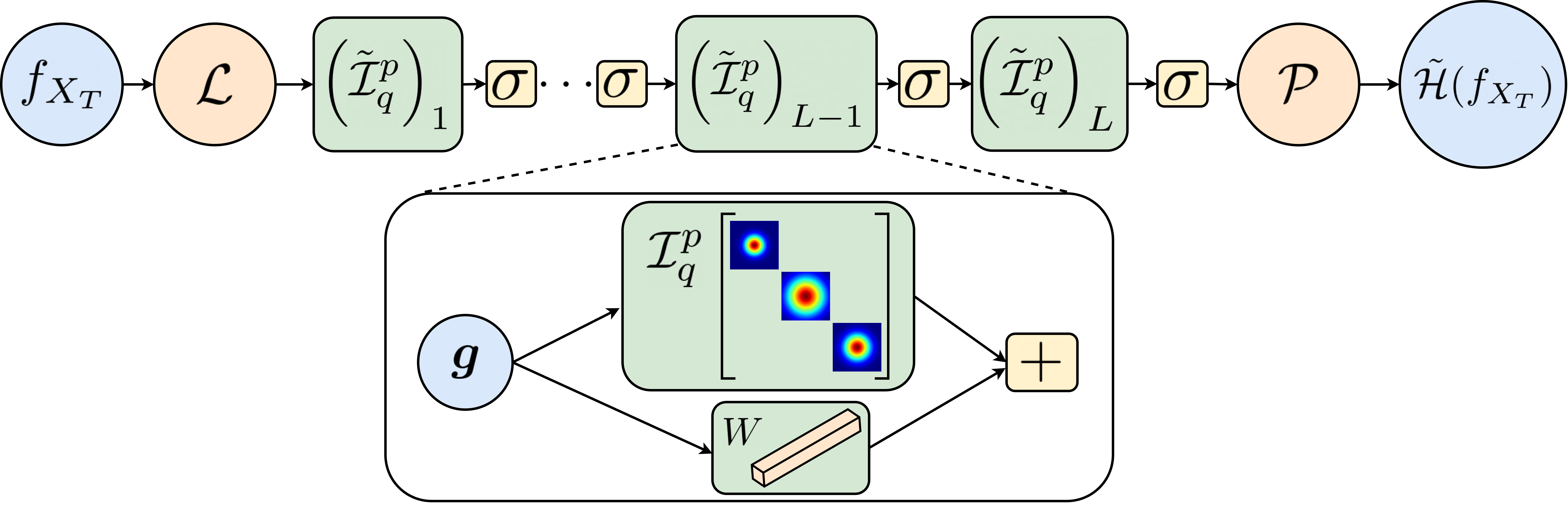
Figure 1: A schematic of the KNO as defined by (17).

We now describe the KNO; a block diagram is shown in Figure 1, while mathematical formulations are shown in (2) and (17).

Integral operators

FNOs use an implicitly-defined, dense, matrix-valued kernel that couples all channels of the architecture. In contrast, the KNO enforces sparsity on this global matrix by utilizing a diagonal matrix-valued kernel. This significantly reduces the number of trainable parameters without degrading accuracy. This amounts to making the simple choices of (i) $p_{0}=p_{1}=\cdots=p_{L-1}=p$ and (ii) choosing $\boldsymbol{K}^{(\ell)}$ as a diagonal kernel. This has the effect of creating $p$ channels. The diagonal elements of $\boldsymbol{K}^{(\ell)}$ are further compressed by making only $q\leq p$ of them trainable, resulting in $q$ trainable kernel parameters per index layer $\ell$. In particular, we choose,

$$\boldsymbol{K}^{(\ell)}=\mathrm{diag}\left(K^{(\ell)}_{I(1)},\ldots,K^{(\ell)}_{I(p)}\right),$$ (8)

where $I:[p]\rightarrow[q]$ is a surjective and monotonic non-decreasing function on $[p]$ (where $[p]=\{p_{0},\ldots,p_{L-1}\}$) , with $I(1)=1$ and $I(p)=q$. We also choose $\Omega_{\ell}=\Omega\subset\mathbb{R}^{d}$ for all $\ell\in[L]$ so that we may use radial kernels. In particular, for $\ell\in[L-1]$, the function $K^{(\ell)}_{i}$ for each $i\in[q]$ is chosen as $K^{(\ell)}_{i}(x,y)=\phi_{\ell,i}(\|x-y\|)$, where $\phi_{\ell,i}:\mathbb{R}\rightarrow\mathbb{R}$ is a radial kernel function with a trainable compact support parameter $\epsilon_{\ell,i}$ to allow flexibility in sparsity; we explicitly provide our choice of $\phi$ in (9), and the final layer $\ell=L$ is described later. We choose $q$ independently of $\ell$, so that these integral operators amount to $(L-1)q$ trainable parameters. Notationally, we will refer to our particular parameterization of the general kernel $\mathcal{I}_{\ell}$ as $(\mathcal{I}^{p}_{q})_{\ell}$:

$$\left(\mathcal{I}_{q}^{p}\right)_{\ell}(\boldsymbol{f}) =\int_{\Omega}\boldsymbol{K}^{(\ell)}(x,y)\boldsymbol{f}(y)dy \boldsymbol{K}^{(\ell)}\textrm{ as in \eqref{eq:KIpq}}.$$

As in many neural operator formulations, we augment these kernel operations at the discrete level with dense cross-channel affine transformations (“pointwise convolutions”) having trainable parameters. We describe this later when we introduce our discretization of the latent space.

2.2 Choosing kernels

Each layer of the KNO contains a set of kernels. In this paper, for all but the last layer, we used compactly-supported radial kernels of the Wendland type. The Wendland kernels are a family of compactly-supported, positive-definite kernels with smoothness class $s$ (up to some finite dimension $d$), and have been used extensively in scientific computing applications [44, 36, 9]; more recently, Wendland kernels have also been used in machine learning applications [14]. The use of Wendland kernels results in a parsimonious parameterization of the KNO, improved training characteristics, spatial sparsity for computational efficiency, and superior accuracy over other choices. Specifically, we used the $C^{4}\left(\mathbb{R}^{d}\right)$ compactly-support radial and isotropic Wendland kernel [42, 43]:

$$\phi_{\epsilon}(r)=\left(\text{ReLU}\left(1-\epsilon r\right)\right)^{6}\left(35(\epsilon r)^{2}+18(\epsilon r)+3\right),$$ (9)

where $\epsilon\in\mathbb{R}^{+}$ is the sole trainable parameter, and $d\leq 3$. The parameter $\epsilon$ serves to both control the flatness of $\phi$ and its region of compact-support: the radius of support $\rho$ is given by $\rho=\frac{1}{\epsilon}$. Since $\phi$ is compactly-supported, a matrix of evaluations of $\phi$ is sparse.

While Wendland kernels can theoretically be used for all layers of a KNO, we found that using an expressive globally-supported kernel within the final integral operator resulted in the best accuracy over a wide range of problems. Specifically, for the last layer we used a spectral mixture kernel constructed as a trainable mixture of two Gaussians [45]: for $\boldsymbol{K}^{(L)}$ as in (8), we defined

$$K_{i}^{(L)}(x,y)=\psi(x-y),\hskip 8.0pt\psi(\tau)=\sum\limits_{r=1}^{2}\lambda_{r}\prod\limits_{p=1}^{d}\cos\left(2\pi\tau_{p}\mu_{r}^{(p)}\right)e^{-2\pi^{2}\tau_{p}^{2}\nu_{r}^{(p)}},$$ (10)

where $\tau_{p}$ is the $p$-th component of $\tau$, and each Gaussian $r=1,2$ has a trainable parameter $\boldsymbol{\mu}_{r}\in\mathbb{R}^{d}$ and trainable covariances (shape parameters) $\nu_{r}^{(1)},\ldots,\nu_{r}^{(d_{y})}$. As with the other layers, we use latent kernels to form the diagonal of the matrix-valued kernel such that the kernel $K^{(L)}_{i}$ has different trainable parameters from $K^{(L)}_{j}$ for $i\neq j$.

Why these kernels?

Unlike existing methods, such as the FNO, the class of kernels used by a KNO can be finely controlled. We leveraged this fine control and investigated compactness of the spectrum of the neural tangent kernel (NTK) matrix of the KNO for different kernel choices. We then chose the KNO architecture whose NTK spectrum indicated the greatest robustness to hyperparameter choices. See Appendix A.2 for details.

2.3 Sampling and outer discretization

Numerically constructing (2) requires sampling from $\nu$ and a discretization of $\|\cdot\|_{\mathcal{Y}}$. To this end, we trained our KNOs using $M$ independent and identically distributed input samples of functions $f^{(m)}\sim\nu$ drawn from $\mathcal{U}$ and the associated output function data $g^{(m)}\coloneqq\mathcal{G}(f^{(m)})$, for $m\in[M]$. We used a training grid, $X_{T}=\{x_{j}\}_{j\in[N_{T}]}\subset\Omega$, to both discretize the input and output functions $f^{(m)}$ and $g^{(m)}$ and to approximate the norm $\|\cdot\|_{\mathcal{Y}}$. Hence, during learning we optimized

$$\|\mathcal{H}-\mathcal{G}\|^{2}_{L^{2}_{\mu}(\mathcal{U},\mathcal{Y})}\stackrel{{\scriptstyle f^{(m)}\sim\nu}}{{\simeq}}\frac{1}{MN_{T}}\sum_{(m,j)\in[M]\times[N_{T}]}\left\|\mathcal{H}(f^{(m)}_{X_{T}})(x_{j})-g^{(m)}(x_{j})\right\|_{2}^{2}.$$ (11)

The input function $f_{X_{T}}$ is defined as a (trainable) kernel interpolant on the training grid:

$$f_{X_{T}}=\sum_{n\in[N_{T}]}c_{n}K(x,x_{n}),$$ (12)

where the $c_{n}$ are determined through a size-$N_{T}$ linear system solve that enforces $f_{X_{T}}(x_{n})=f(x_{n})$. This interpolant allows for evaluation of $f$ off of the training points $X_{T}$, and in particular, at the quadrature points to be introduced shortly. We chose the kernel as $K(x,y)=\phi(\|x-y\|)$ from (9), which ensured that the linear system was sparse and well-conditioned. We emphasize that our choice to evaluate the outputs of $\mathcal{H}$ at $X_{T}$ was only to enable simple training of our KNOs; for generalization and super-resolution, one can evaluate the output of $\mathcal{H}$ on any desired grid.

2.4 Latent space discretization: Quadrature on general domains

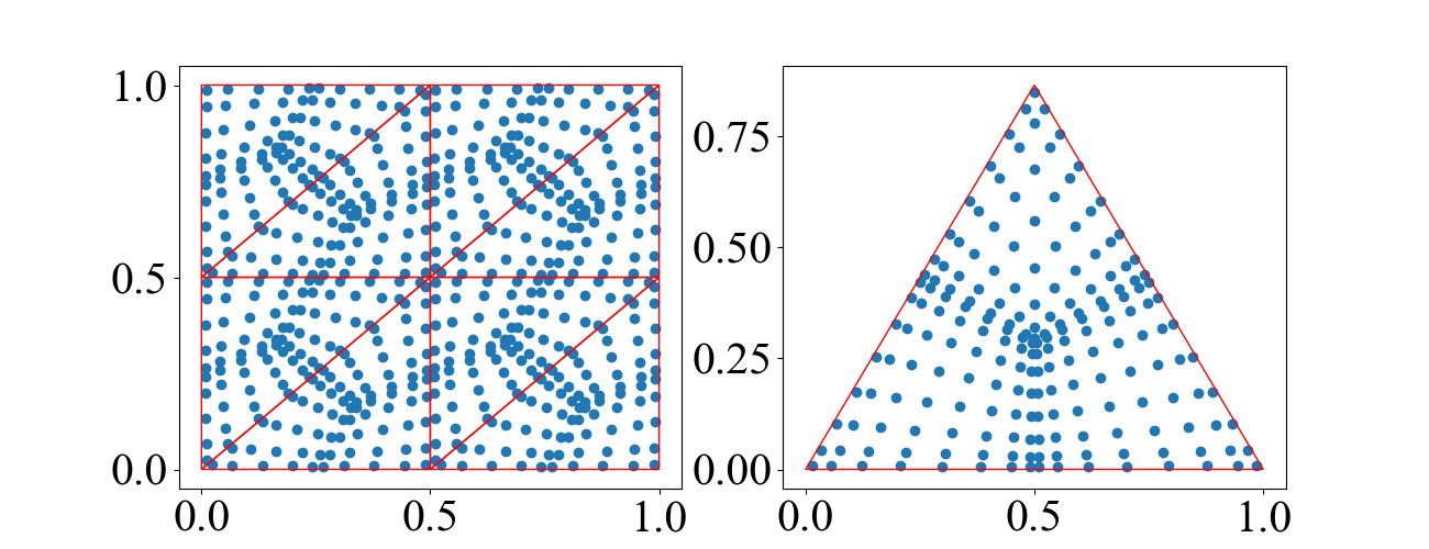
Figure 2: Clustered quadrature points on $[0,1]^{2}$ (left) and a reference triangle (right).

In order to propagate $f_{X_{T}}$ through $\mathcal{H}$ in (11), one must discretize all the integral operators; we accomplished this with quadrature. This first requires that we evaluate the kernel interpolant (12) at some set of quadrature points (described further below). This KNO methodology of directly discretizing the integrals via quadrature is a crucial difference compared to other neural operator approaches. Consider the discretization of an integral operator $\int_{\Omega}K(x,y)f(y)d\mu(y)$ that acts on a scalar-valued function $f:\mathbb{R}^{d}\to\mathbb{R}$; the generalization to vector-valued functions is straightforward. Then given a quadrature rule $\{w^{q}_{i},y^{q}_{i}\}_{i=1}^{N_{Q}}$, where $w^{q}_{i}\in\mathbb{R}$ are quadrature weights and $y^{q}_{i}\in\mathbb{R}^{d}$ are quadrature points, the quadrature-based discretization of a KNO integral operator is

$$\int_{\Omega}K(x,y)f(y)d\mu(y)\approx\sum\limits_{i=1}^{N_{Q}}w^{q}_{i}K\left(x,y^{q}_{i}\right)f(y^{q}_{i}).$$ (13)

In general, the choice of quadrature rule is dependent on the domain $\Omega$ and $\mu$ (which is in turn application dependent) and should consist of quadrature points that allow for stable integration. For non-periodic kernels (which we use) this typically implies quadrature points that are clustered towards the boundary $\partial\Omega$. To accomplish this, we tesselated $\Omega$ with a simplicial mesh that divided $\Omega$ into some set of nonoverlapping subdomains $\Omega_{\ell}$, $\ell=1,\ldots,N_{\Omega}$ such that

$$\int_{\Omega}K(x,y)f(y)d\mu(y)=\sum\limits_{\ell=1}^{N_{\Omega}}\int_{\Omega_{\ell}}K(x,y)f(y)d\mu(y).$$ (14)

Following standard scientific computing practices [18, 6]we discretized (14) using a quadrature rule for each of the subdomains $\Omega_{\ell}$ affinely-mapped from a symmetric quadrature rule on a standard (“reference”) simplex $\Omega_{\textit{ref}}$ in $\mathbb{R}^{d}$ [12]; see Figure 2. This simplified to the Gauss-Legendre rule in 1D.

2.4.1 Cross-channel affine transformations

As in other neural operators [25], we also augmented each layer of the KNO with a cross-channel affine transformation (i.e., an MLP dense layer), sometimes called a “pointwise convolution”. The output of this operation is added to the output of the integral operator. Formally, we use the modified integral operators that explicitly act on and output vectors of function evaluations on $X_{Q}\coloneqq\{y^{q}_{i}\}_{i\in[N_{Q}]}$:

$$\left(\tilde{\mathcal{I}}^{p}_{q}\right)_{\ell}\boldsymbol{\tilde{g}}_{\ell} =\boldsymbol{\tilde{g}}_{\ell}W_{\ell}+\boldsymbol{1}_{N_{Q}}(b_{\ell})+\left(\left(\mathcal{I}^{p}_{q}\right)_{\ell}\boldsymbol{\tilde{g}}_{\ell}\right)\big{|}_{X_{Q}}, \ell \in[L-1]$$ (15)

$$\left(\tilde{\mathcal{I}}^{p}_{q}\right)_{L}\boldsymbol{\tilde{g}}_{L} =\left(\left(\mathcal{I}^{p}_{q}\right)_{L}\boldsymbol{\tilde{g}}_{L}\right)\big{|}_{X_{T}},$$ (16)

where $\boldsymbol{\tilde{g}}_{\ell}\in\mathbb{R}^{N_{Q}\times p}$ denotes evaluations of the function $\boldsymbol{g}_{\ell}:\Omega\to\mathbb{R}^{p}$ on $X_{Q}$, and $W_{\ell}\in\mathbb{R}^{p\times p}$ and $b_{\ell}\in\mathbb{R}^{1\times p}$ are trainable weights. Note that we abuse notation in the term $\left(\left(\mathcal{I}^{p}_{q}\right)_{\ell}\boldsymbol{\tilde{g}}_{\ell}\right)\big{|}_{X_{Q}}$ by passing the vector $\boldsymbol{\tilde{g}}$ evaluated at quadrature points to the integral operator (rather than a function). The final discretized integral operator outputs values on the training grid $X_{T}$ for use in evaluating the loss. We found that removing these pointwise convolutions entirely was detrimental to accuracy.

2.4.2 Lifting and projection operators

As with other neural operators, we used standard multilayer perceptrons (MLPs) to parameterize the lifting and projection operators $\mathcal{L}$ and $\mathcal{P}$ that act on discretized inputs. Our lifting operator $\mathcal{L}$ is given by $\mathcal{L}f=\sigma\left(\left(\left.f\right|_{X_{Q}}\oplus X_{Q}\right)W+\boldsymbol{1}_{N_{Q}}b\right)$, where $\oplus$ indicates concatenation, $W\in\mathbb{R}^{(d_{u}+\text{dim}(\Omega_{u}))\times p}$ and $b\in\mathbb{R}^{1\times p}$ are trainable, $\sigma$ is an activation function, and $X_{Q}$ now represents a matrix of quadrature points. An MLP was also used to parameterize the projection operator $\mathcal{P}$ that combines all the $p$ channels of the hidden layers to produce a single approximation of the output function(s). This MLP consisted of two consecutive $p$-width dense layers ($\mathcal{A}:\mathbb{R}^{p}\rightarrow\mathbb{R}^{p}$) with nonlinear activation functions and one dense layer with width equal to $d_{y}$ ($\mathcal{A}:\mathbb{R}^{p}\rightarrow\mathbb{R}^{d_{y}}$) that did not use an activation function. We use the GeLU activation function in all cases [15]; see Appendix A.5 for more details. In summary, the discretized KNO $\widetilde{\mathcal{H}}$ that we used to numerically construct $\mathcal{H}$ in (2) can be written as a function that takes in $f_{X_{T}}$ and returns an approximation to the output function $\mathcal{H}(f)$ evaluated at $X_{T}$:

$$\widetilde{\mathcal{H}}(f_{X_{T}})=\left(\mathcal{P}\circ\sigma\circ\left(\tilde{\mathcal{I}}^{p}_{q}\right)_{L}\circ\sigma\circ\left(\tilde{\mathcal{I}}^{p}_{q}\right)_{L-1}\circ\sigma\circ\ldots\sigma\circ\left(\tilde{\mathcal{I}}^{p}_{q}\right)_{1}\circ\mathcal{L}\right)(f_{X_{T}})$$ (17)

3 Results

In this section, we describe the numerical experiments we used to compare the accuracy of KNOs, on benchmark problems obtained from [29], with the accuracy of state-of-the-art neural operators; following [29], we present benchmarks on both tensor-product domains, (all of which used boundary-anchored equidistant grids) and irregular domains (which used triangle meshes). All of the KNO models were trained using the Adam optimizer [21] with a cyclic cosine annealing learning rate schedule. Other technical details are described in Appendices A.3–A.5. We measured the accuracy of our KNOs by computing the mean and standard deviation of the $\ell_{2}$ relative errors of each KNO obtained from nine different training runs: three separate train/test splits, each with three different random model parameter initializations. These errors were compared to those of DeepONets, POD-DeepONets, and FNOs all as reported in [29], and kernel/GP-based methods (denoted KM) as reported in [2]; see Appendix A.6.1 for the architecture details. All errors are reported in Table 1, and all parameter counts are given in Table 2. We used the normalization procedure described in [29, Section 3.4] in all cases except the KM.

3.1 Tensor-Product Domains

Table 1: Percent $\ell_{2}$ relative errors. All non-KNO errors were reported from the literature [29, 2]. The last two rows correspond to irregular domains; these used the dgFNO+ rather than the FNO.

PDE	KM	DeepONet	POD-DeepONet	FNO	KNO
Burgers’ Equation	2.15	$2.15\pm 0.09$	$1.94\pm 0.07$	$1.93\pm 0.04$	$\mathbf{0.52\pm 0.08}$
Advection (I)	$\mathbf{2.15\mathrm{e}{-13}}$	$0.22\pm 0.03$	$0.04\pm 0.00$	$0.66\pm 0.10$	$0.015\pm 0.01$
Navier-Stokes	–	$1.78\pm 0.02$	$1.71\pm 0.03$	$1.81\pm 0.02$	$\mathbf{1.02\pm 0.15}$
Darcy (Continuous)	–	$1.36\pm 0.12$	$1.26\pm 0.07$	$1.19\pm 0.05$	$\mathbf{0.91\pm 0.05}$
Darcy (PWC)	2.75	$2.91\pm 0.04$	$2.32\pm 0.03$	$2.41\pm 0.03$	$\mathbf{1.57\pm 0.06}$
Darcy (triangular)	-	$0.43\pm 0.02$	$0.18\pm 0.02$	$1.00\pm 0.03$	$\mathbf{0.12\pm 0.01}$
Darcy (triangular-notch)	-	$2.64\pm 0.02$	$1.00\pm 0.00$	$7.82\pm 0.03$	$\mathbf{0.55\pm 0.04}$

3.1.1 Burgers’ Equation

We first considered Burgers’ equation in one dimension with periodic boundary conditions:

$$\frac{\partial u}{\partial t}+u\frac{\partial u}{\partial x}=\nu\frac{\partial^{2}u}{\partial x^{2}},\quad x\in(0,1),\quad t\in(0,1),$$

with the viscosity coefficient fixed to $\nu=0.1$. Specifically, we learned the mapping from the initial condition $u(x,0)=u_{0}(x)$ to the solution $u(x,t)$ at $t=1$, i.e., $\mathcal{G}:u_{0}\mapsto u(\cdot,1)$. The input functions $u_{0}$ were generated by sampling $u_{0}\sim\mu$, where $\mu=\mathcal{N}(0,625(-\Delta+25I)^{-2})$ with periodic boundary conditions, and the Laplacian $\Delta$ was numerically approximated on $X_{T}$. The solution was generated as described in [25, Appendix A.3.1]. The full spatial resolution of this dataset was 8192, but the models were trained and evaluated on input-output function pairs both defined on the same downsampled 128 grid (as were the errors). 1000 examples were used for training and 200 for testing.

In this problem, the KNO showed the best accuracy of all the models (Table 1) and achieved roughly a four-fold improvement over the next best model (the FNO), while requiring an order of magnitude fewer parameters than the FNO (Table 2).

3.1.2 Advection Equation

Next, we studied an operator learning problem associated with the 1D advection equation given by

$$\frac{\partial u}{\partial t}+\frac{\partial u}{\partial x}=0,\quad x\in[0,1],\quad t\in[0,1],$$

with a periodic boundary condition $u(0,t)=u(1,t)$. Specifically, we learned the mapping $\mathcal{G}:u_{0}\mapsto u(\cdot,0.5)$ [29, Case (I), Section 5.4.1]. The initial condition was a square wave with center, width and height uniformly sampled from $[0.3,0.7]$, $[0.3,0.6]$, and $[1,2]$ respectively. The spatial resolution for this data was fixed to 40, and we generated 1000 training and testing examples. The KNO again outperformed all the neural operators (Table 1), but was unable to match the kernel method (KM), which used a linear kernel to recover the linear operator $\mathcal{G}$. We believe it should be possible to obtain the same accuracy with the KNO by removing nonlinearities as appropriate; however, we leave an exploration of problem-specific architectures for future work and focus on the generalizable and flexible architecture reported here.

3.1.3 The Incompressible Navier-Stokes Equations

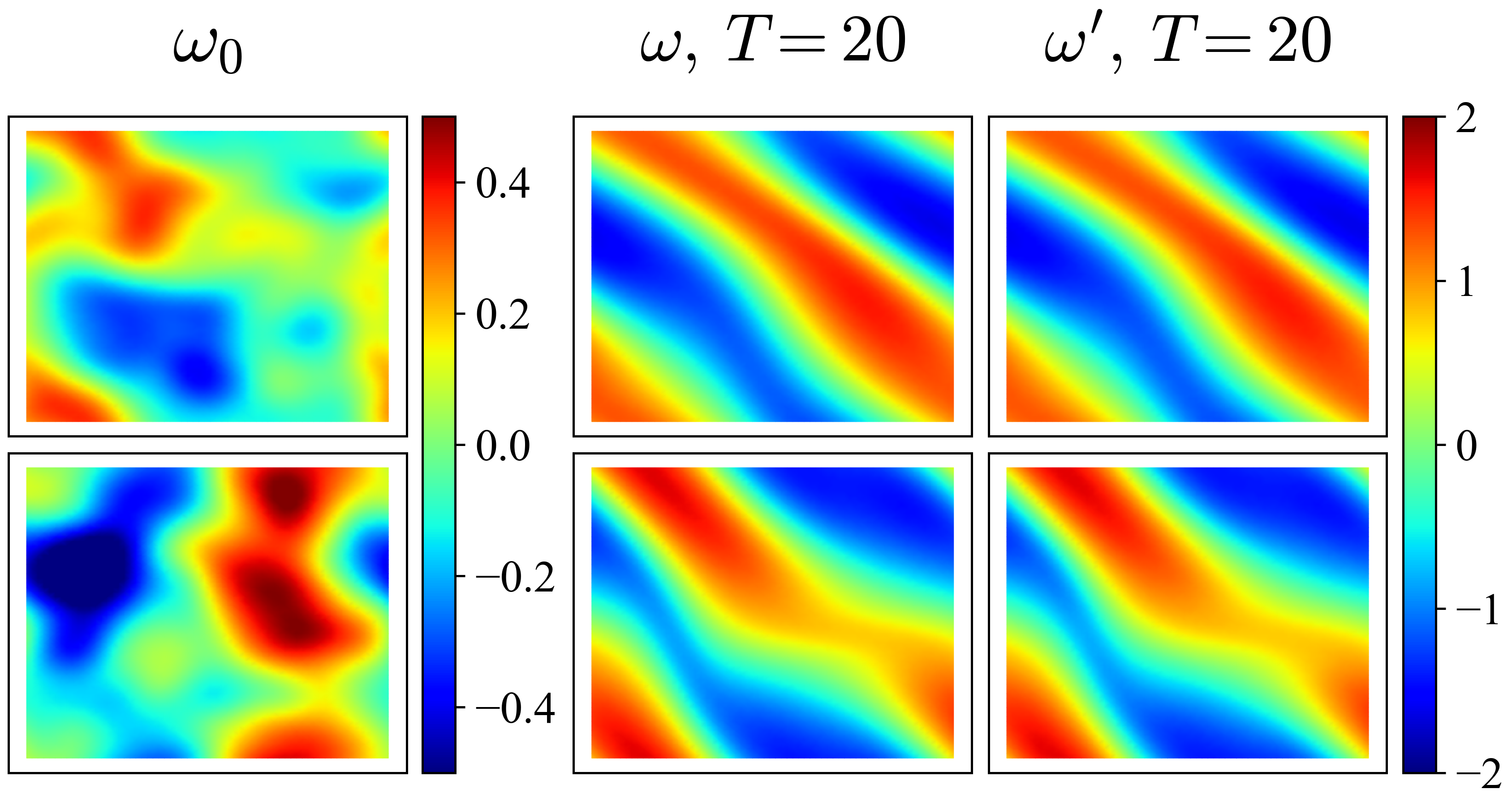
Figure 3: Solutions of the Navier-Stokes problem 3.1.3 on a test example. We show the initial vorticity (left), the solution at $t=20\Delta t$ (center), and the prediction at $t=20\Delta t$ (right).

In this test, we learned a solution operator for the 2D incompressible Navier-Stokes equations given in vorticity-velocity form on the spacetime domain $[0,1]^{2}\times[0,T]$:

$$\frac{\partial\omega}{\partial t}+\mathbf{u}\cdot\nabla\omega=\nu\Delta\omega+f,\ \ \omega(x,0)=\omega_{0}(x),$$

where $\omega(x,y,t)$ is the fluid vorticity, $\mathbf{u}(x,y,t)$ is the velocity, $\nu=0.001$ is the viscosity, and $\nabla\cdot\mathbf{u}=0$; we enforced periodic boundary conditions on $\omega$. The forcing term $f$ was prescribed to be

$$f(x,y)=0.1\sin(2\pi(x+y))+0.1\cos(2\pi(x+y)).$$

We learned the mapping from the set of functions $\{\omega(x,y,j\Delta t)\}$, $j=0,\ldots,9$ to the function $\omega(x,y,20\Delta t)$ by passing the first ten steps as a vector-valued input to the KNO. The input functions were generated by sampling as $\omega_{0}\sim\mathcal{N}(0,7^{3/2}(-\Delta+49I)^{-2.5}$), and a numerical solution was obtained as in [25, Section A.3.3]. The input and output function pairs were downsampled from $256\times 256$ to a resolution of $64\times 64$ before using them to train and evaluate the neural operators. We used 1000 examples for training and 200 for testing. Once again, the KNO outperformed all other models (Table 1), while requiring fewer than $10,000$ trainable parameters (Table 2).

3.1.4 Darcy Flow

Next we used KNOs to learn two operators $\mathcal{G}:K\mapsto h$ associated with 2D Darcy flow

$$-\nabla\cdot(K(x,y)\nabla h(x,y))=f(x,y),\quad(x,y)\in\Omega.$$

on the $\Omega=[0,1]^{2}$. For case (1), the permeability field was generated via $K=\psi(\mu)$, where $\mu\sim\mathcal{N}(0,(-\Delta+9I)^{-2})$, and $\psi$ is a function that pointwise converts all non-negative values to $12$ and all negative values to $3$. We henceforth refer to this problem as “Darcy (PWC)”. Case (2) involved generating continuous permeability fields using a Gaussian process parameterized with a zero mean and Gaussian covariance kernel; see [25] for details. We refer to this problem as “Darcy (cont.)”. Both problems used 1000 training functions and 200 test functions.

The Darcy (PWC) solutions were computed on a $421\times 421$ grid [29] and the input and output training functions were subsampled from this grid to a $29\times 29$ grid. The Darcy (cont.) solutions [29] were obtained using the Matlab PDE Toolbox on an unstructured mesh with 1,893 elements, in which Neumann and Dirchlet boundary conditions were imposed on the top and bottom boundaries, and the left and right boundaries respectively. The solutions $h$ were then linearly interpolated from the mesh to the same uniform $20\times 20$ grid upon which $K$ was originally defined so that both functions shared the same discretization.

The KNO achieved under $1\%$ error on the Darcy (cont.) problem, once again showing the best accuracy among all the neural operators tested. Further, in Darcy (PWC), the KNO achieved a $30\%$ lower error than the second-best model (FNO) while requiring over two orders of magnitude fewer trainable parameters than FNO and DeepONet and almost two orders of magnitude fewer trainable parameters than POD-DeepONet.

Table 2: Parameter counts for the models in Table 1 provided wherever available. For some we made conservative estimates (detailed in Appendix A.6.2), which are marked with an asterisk. The number of KNO parameters is determined by the hyperparameter choices detailed in Table 3.

PDE	DeepONet	POD-DeepONet	FNO	KNO
Burgers’ Equation	148,865	53,664	287,425	34,307
Advection (I)	–	86,054	–	30,083
Darcy (PWC)	715,777	631,155	1,188,353	6,723
Darcy (Continuous)	–	–	–	26,179
Navier-Stokes Equations	–	–	*414,517	7,011
Darcy (triangular)	*88,777	50,208	*532,993	25,731
Darcy (triangular-notch)	88,777	230,796	532,993	25,507

3.2 Irregular Domains

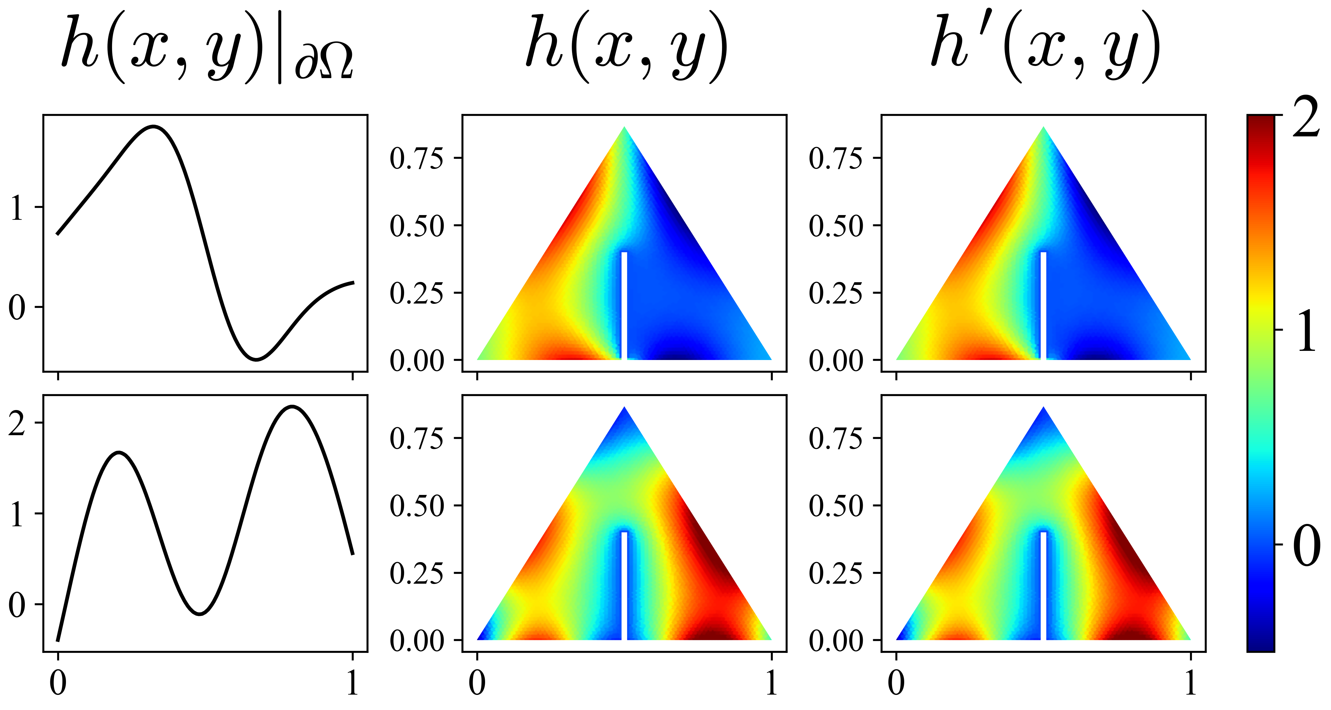
Figure 4: Solutions of the Darcy (triangular-notch) problem 3.2.2. We show two input functions (left), solution functions (middle), and the KNO predictions (right).

Finally, we examined two Darcy flow problems where the input and output functions were both discretized on an irregular spatial domain. Specifically, as in [29], we learned the mapping from the Dirichlet boundary condition to the pressure field over the entire domain, i.e., the operator $\mathcal{G}:\left.h(x,y)\right|_{\partial\Omega}\mapsto h(x,y)$. We report the dgFNO+ variant’s performance under the FNO column since it can tackle both irregular geometries and different input and output domains. Here $K(x,y)=0.1$ and $f=-1$. The input functions $\left.h(x,y)\right|_{\partial\Omega}$ for both problems were generated as follows. First, we generated $\tilde{h}(x)\sim\mathcal{GP}(0,\mathcal{K}(x,x^{\prime})),\quad\mathcal{K}(x,x^{\prime})=\exp[-\frac{(x-x^{\prime})^{2}}{2l^{2}}]$, where $l=0.2$ and $x,x^{\prime}\in[0,1]$. We then simply evaluated $\tilde{h}(x)$ at the $x$-coordinates of the boundary points of each unstructured mesh to obtain $h(x,y)\big{|}_{\partial\Omega}$. The Matlab PDE Toolbox was used both to generate unstructured meshes and numerical solutions [29]. Both problems used 1900 training examples and 100 test examples.

3.2.1 Darcy (triangular)

This problem utilized an 861 vertex unstructured mesh with 120 points lying on the boundary; see [29] (Figure S2 (c)). Once again, the KNO showed the best accuracy of all neural operators on this domain, partly illustrating the effectiveness of our quadrature rule (see Section 2.4). As in the other test cases, the KNO required far fewer trainable parameters than existing neural operators.

3.2.2 Darcy (triangular-notch)

This problem involved removing a small notch from the triangular domain [29] (see Figure 4). The mesh contained 2,295 vertices with 260 of those on the boundary. Again, the KNO outperformed the other models; it was almost twice as accurate as the next best model, the POD-DeepONet, with an order of magnitude fewer parameters than dgFNO+. The results here underscore KNO’s flexibility, both in handling different input and output spaces and in tackling irregular geometries.

4 Conclusion

We presented the kernel neural operator (KNO), a novel, simple, and transparent architecture that leverages kernel-based deep integral operators discretized by numerical quadrature. The use of explicit, closed-form, diagonal, matrix-valued kernels allowed the KNO to achieve superior accuracy with far fewer trainable parameters than other neural operators (on both regular and irregular domains). We found that compactly-supported kernels used throughout (save the final layer) were the optimal choice to obtain a general purpose architecture well-suited to a wide variety of operator learning problems. In our view, our results also indicate that it may be possible to achieve similar parameter counts (and possibly relative errors) with other neural operators such as DeepONet and the FNO, albeit with architecture tuning, careful training, and problem-specific initializations.

For future work, we will prove the universal approximation capabilities of the KNO and leverage the closed form kernels to derive rigorous error estimates for the approximation of PDE solution operators. We will also explore interpretable lifting and projection operators, problem-specific architectures (for instance, for linear operators), novel quadrature schemes, and other types of problem-dependent kernels not discussed in this work. We anticipate that the KNO will be widely applicable to a variety of machine learning tasks beyond approximating PDE solution operators. We plan to explore these in future work as well.

Appendix A Appendix

A.1 Zero-shot super-resolution

As every layer in the KNO is composed of function-space operations, the KNO can achieve zero-shot super resolution, i.e., it can produce operator solutions at arbitrary resolutions without retraining, much like the FNO. This is visualized in Figure 5.

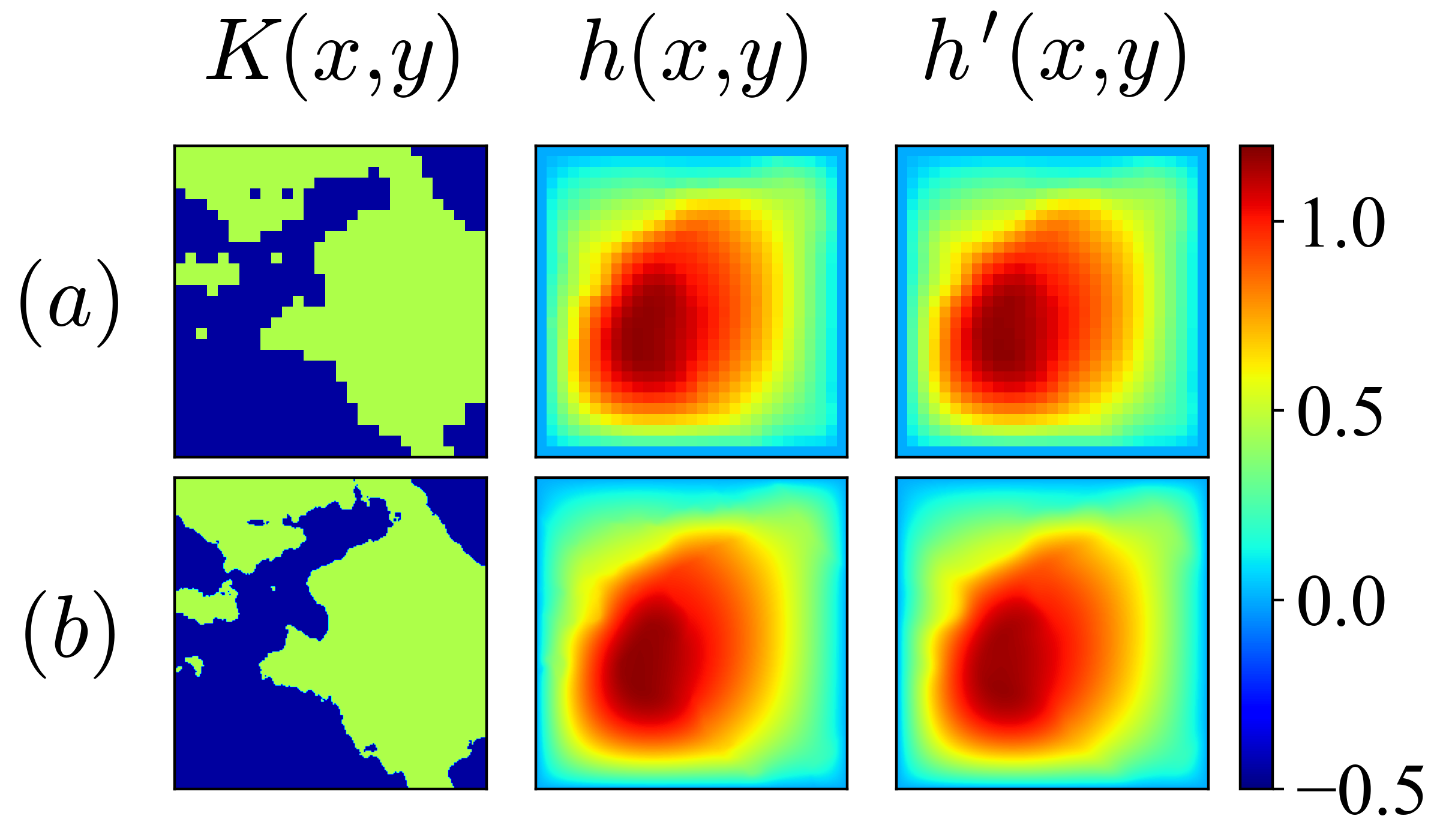
Figure 5: An illustration of zero-shot super-resolution. The KNO was trained on the Darcy (PWC) dataset using a $29\times 29$ grid (row a). It was then evaluated at a resolution of $211\times 211$ (row b). We show the permeability field input (left), the actual pressure field (middle), and the predicted pressure (right).

A.2 Other kernel choices

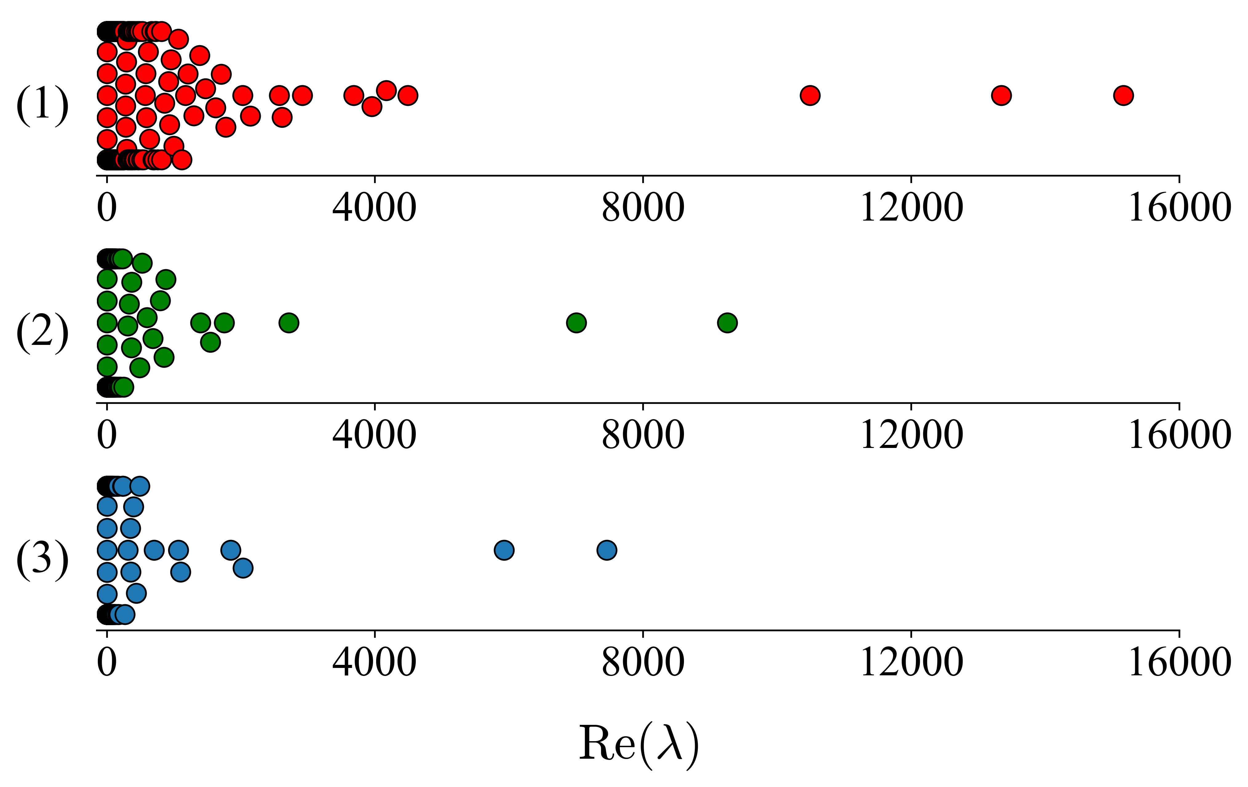
Figure 6: Eigenvalues of the neural tangent kernel (NTK) for three choices of kernels: (1) Gaussian kernels for $\left(\mathcal{I}^{p}_{q}\right)_{k}$, $k=1,\ldots,L$; (2) $C^{4}(\mathbb{R}^{3})$ Wendland kernels for$\left(\mathcal{I}^{p}_{q}\right)_{k}$, $k=1,\ldots,L-1$ and a Gaussian kernel for $\left(\mathcal{I}^{p}_{q}\right)_{L}$; and (3) $C^{4}(\mathbb{R}^{3})$ Wendland kernels for$\left(\mathcal{I}^{p}_{q}\right)_{k}$, $k=1,\ldots,L-1$ and a Gaussian spectral mixture kernel for $\left(\mathcal{I}^{p}_{q}\right)_{L}$.

As mentioned previously, we also explored the use of other kernels, enumerated below, within our integral operators, however the KNO architecture reported in the main text out-performed all of the other kernels tested.

1. Gaussians everywhere (overfitting): When isotropic Gaussian kernels $\phi(x,x^{\prime})=e^{\epsilon^{2}\|x-y\|^{2}_{2}}$ were used throughout the KNO, we found that the resulting architecture tended to achieve low training error and high test error, while also being highly sensitive to the initial random seed used to optimize the KNO.

2. Wendland everywhere (higher training and test errors): When we used Wendland kernels everywhere, we found that the resulting architecture had significantly higher training and test errors than using Wendland kernels almost everywhere and a spectral mixture kernel at the end. This experiment revealed to us that using a kernel that was not compactly-supported for the final integral operator was important for accuracy. This is possibly due to the fact that our final integral operator simply did not use a cross-channel affine transformation (aka pointwise convolution).

3. Wendland almost-everywhere, Gaussian for $\left(\mathcal{I}^{p}_{q}\right)_{L}$: This choice of kernels produced excellent training and test accuracy and was relatively robust to choices in the other hyperparameters, but produced higher errors than using the spectral mixture kernel for $\left(\mathcal{I}^{p}_{q}\right)_{L}$.

In order to quantify the differences between these choices, we computed the eigenvalue spectra of the neural tangent kernel (NTK) matrix for the final KNO architecture, for cases (1) and (3) above; case (2) produced reasonable spectra but lowered accuracy (not shown). The spectra of these NTK matrices are shown in Figure 6; in general, more tightly clustered eigenvalues of the NTK matrix are indicative of fewer local minima and a lower tendency to overfit. We see that the Gaussian results in a spectrum with a very large range, while the Wendland + Gaussian choice results in a much tighter spectrum; the Wendland + spectral mixture choice results in the tightest spectrum of all. It is possible that stable kernel evaluation via a Hilbert-Schmidt decomposition might improve the Gaussian’s NTK spectra [10], but we save such an exploration for future work.

We also believe Wendland kernels were vital in the kernel interpolant that transfers data to the quadrature points as their finite smoothness and corresponding sparse interpolation matrices allowed us to avoid the exponential ill-conditioning inherent to interpolation on boundary-anchored equispaced grids. The Gaussian kernel, on the other hand, is infinitely-smooth and capable of exponential convergence on infinitely-smooth target functions. Its corresponding linear system hence suffers from exponential ill-conditioning (much like polynomial Vandermonde matrices); this follows directly from the impossibility theorem [34, 1].

We also ran another experiment (results not shown) to investigate the impact of limited smoothness of the Wendland kernels on efficacy. Specifically, we replaced the Wendland kernels with $C^{4}(\mathbb{R}^{3})$ Matérn kernels, which are finitely-smooth but not compactly-supported. We observed worse errors in all our experiments using Matérn kernels over Wendland kernels (but still better results than using the Gaussian everywhere). It may be possible to understand this in terms of the Fourier transforms of these kernels. In general, in the context of interpolation, the rate of decay of the Fourier transform of a kernel can affect its approximation power [9]. In this context, we believe it affects trainability also. Wendland kernels, being compactly-supported, have Fourier transforms with heavy frequency tails (by the Fourier uncertainty principle), thus carrying more information. In contrast, Gaussians and even other less smooth Matérn kernels have more concentrated Fourier transforms with fast decay (exponential in the frequency for Gaussian kernels, algebraic for the Matérn kernels), which likely results in a loss of information during training. In future work, we plan to apply Fourier analysis tools to further understand and clarify this intuition.

A.3 KNO sparsity

We also tracked the learned sparsity in the KNOs, specifically the average number of zeros in each kernel evaluation matrix formed by the Wendland kernels. This metric roughly converged to $20\%$, $20\%$, $26\%$, $27\%$ and $23\%$ for the tensor-product domain datasets in the order by which they are listed in Table 1. Interestingly, for the problems on irregular domains, we observed lower sparsity percentages, $6\%$ and $4\%$, for the Darcy (triangular) and Darcy (triangular-notch) problems respectively. It is possible that this was because the triangular Darcy problems involved mapping boundary conditions to solutions over the full domain. We leave a deeper exploration of the connection between sparsity and the operator learning problem for future work.

A.4 Ablation studies

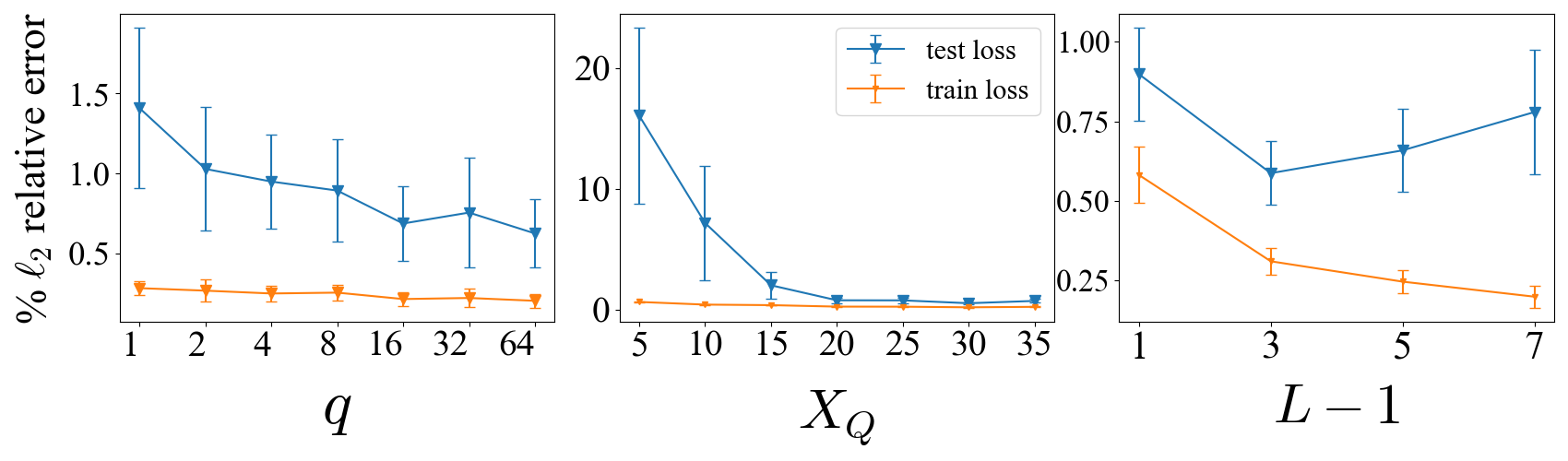
Figure 7: Ablation Study for Burgers’ Equation. On the left the number of trainable kernels $q$ per integration block (for $p=64$) was systematically varied with a constant architecture otherwise ($X_{Q}=30$ and $L-1=6$). The number of Gauss-Legendre quadrature points (center) were scaled in the same capacity with $p$ and $q$ fixed to $64$ and $L-1=6$. The depth (right) was also scaled with $p,q=64$ and $X_{Q}=30$.

To verify the robustness of our results under training, we also conducted ablation studies on Burgers’ equation. We focused on the ratio between the number of trainable kernels $q$ as compared and the channel lift size $p$, on the number of Gauss-Legendre quadrature points employed, and on the model depth; that is, the total number of integration blocks excluding the evaluation block ($L-1$). The results are shown in Figure 7.

Figure 7 (left) shows that while the best results are obtained with $q=p$, smaller values of $q$ may also suffice, i.e., one may be able to use fewer trainable parameters than channels, allowing for significant reductions in computational cost. It is also likely that this can be done with the FNO family of neural operators. Figure 7 (middle) also shows a relative insensitivity of our results to the number of quadrature points for the datasets used in this work; however, it is not unreasonable to expect some relationship between the number of spatial samples of the input and output functions and the number of quadrature points. We plan to explore this connection in future work. Finally, Figure 7 (right) shows that the depth of the KNO was much more important, especially for generalization. KNOs with more layers tended to overfit on this 1D problem. However, it is plausible that there is an optimal depth for a given dataset in a particular spatial dimension. We leave such an exploration for future work also.

A.5 Important architectural and training details for the KNO

A.5.1 Initialization and regularization

We initialized all trainable parameters associated with kernels by sampling $\mathcal{N}(1,0.01)$ and applied a softplus transform to enforce that all kernel shape parameters were positive. We also include a very mild $\ell_{2}$ regularization to the shape parameters in the loss term to encourage sparsity but did not find this to substantially impact convergence.

A.5.2 Quadrature points

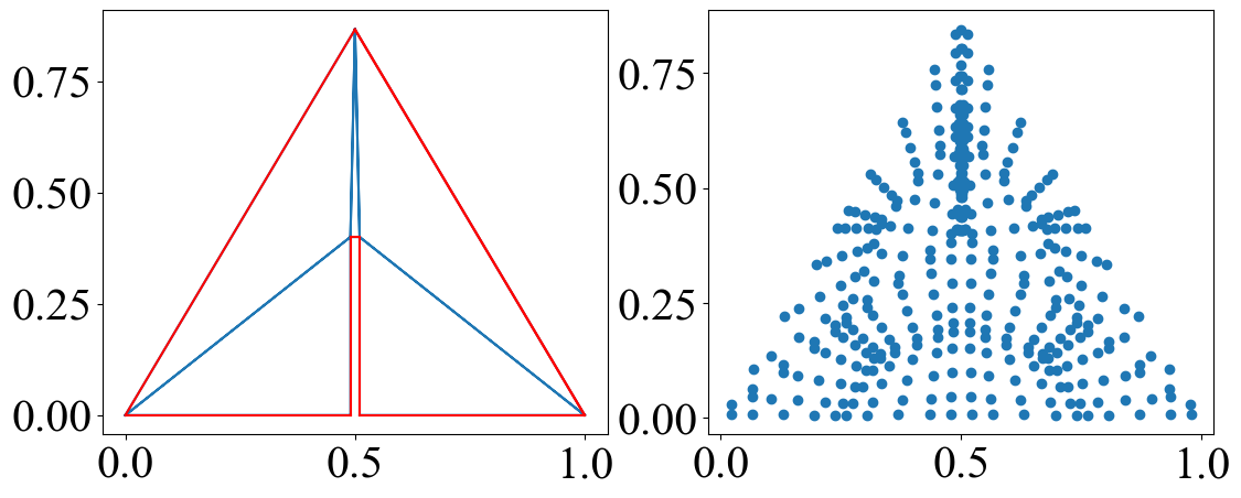
Figure 8: On the right is a quadrature rule for the Darcy (triangular-notch) problem, created by mapping the reference triangle’s rule 2 defined at $\left[(0,0),(1,0),(\frac{\sqrt{3}}{2},0.5)\right]$, to a five triangle Delaunay mesh (left) over the domain. The cut out ‘notch’ is defined by the vertices $\left[(0.49,0),(0.51,0),(0.49,0.4),(0.51,0.4)\right].$

We now briefly present details on the quadrature points used in the different operator learning problems. For the 2D examples, we took the approach of subdividing the domain into some number of triangles, then mapped the integrals on each triangle back to our reference triangle (as was mentioned previously).

1. As was mentioned previously, all 1D examples used Gauss-Legendre points defined on $[-1,1]$. We simply transformed the Gauss-Legendre points to the domain of interest in this case.

2. For the Darcy (PWC) and Navier-Stokes problems, we subdivided the domain $[0,1]^{2}$ into four squares, then further subdivided each square into two triangles, for a total of eight triangles.

3. For the Darcy (cont.) problem, we simply used two triangles.

4. For the Darcy (triangular-notch) problem, we created a five triangle Delaunay mesh over the whole domain; see Figure 8.

5. For the Darcy (triangle) problem, the domain matched our reference triangle, and so no further subdivision or mapping was used.

A.5.3 Hyperparameter choices

Table 3: This table denotes our chosen configuration for KNO on each dataset. An asterisk indicates a hyperparameter that when increased also increases the total number of trainable parameters. Here $X_{Q}$ is the total number of quadrature nodes, $L-1$ is the ‘depth’ as referred to previously and $q$ is effectively the number of trainable kernels relative to the channel lift dimension $p$.

	$X_{Q}$	$(L-1)^{*}$	$q^{*}$	$p^{*}$
Burgers’ Equation	30	6	64	64
Advection (I)	32	5	64	64
Darcy (PWC)	864	4	16	32
Darcy (Continuous)	294	4	64	64
Navier-Stokes	384	4	16	32
Darcy (triangular)	300	4	32	64
Darcy (triangular-notch)	375	4	16	64

The optimal hyperparameters for the KNO on each dataset are shown in Table 3. These hyperparameters were tuned manually via trial and error. The following are some relevant observations:

(1) Setting the depth $L-1=4$ was the most reliable choice with a few exceptions, namely the Advection (1) and Burgers’ equation problems, where the optimal depth increased to 5 and 6 respectively. Usually, increasing the depth resulted in training instability and/or overfitting. However, it is possible that more complicated residual connections or an addition of batch normalization between integration layers could allow for deeper models to be more successful. The KNO is well-suited to such augmentations since it innately possesses a very small number of trainable parameters per layer.

(2) We found that altering the MLP layer width to a value other than $p$ provided no benefit.

(3) In several instances, we were able to reduce $q<p$, which not only reduced trainable parameters, but also provided regularization, slightly improving test accuracy. These problems were: Darcy (PWC) where $q=16$ and $p=32$, the Navier-Stokes equations ($q=16$ and $p=32$), Darcy (triangular) ($q=32$ and $p=64$), and Darcy (triangular-notch) ($q=16$ and $p=64$).

(4) On the 1D problems, we observed optimal performance with $\sim 30$ quadrature nodes. In contrast, this number was $\sim 300-400$ for the 2D datasets, reflecting the exponential relationship between the number of quadratures nodes and the spatial dimension. A slight exception to this is the Darcy (PWC) problem, in which KNO performed optimally with $\sim 900$ nodes. This is potentially a result of the piecewise constant nature of the input function, which necessitates more quadrature nodes to resolve the discontinuities. Here (and in general) an adaptive, problem specific quadrature rule could be beneficial and potentially enable us to reduce $X_{Q}$ further. We leave such an exploration for future work.

A.5.4 Training details

All models were trained on either an NVIDIA GeForce RTX 2080 Ti or an NVIDIA GeForce RTX 4080. We found that freeze-training (i.e. training kernel-based layers independently back to front) prior to training the full model hastened its convergence and so used this tactic quite often for the sake of convenience. More specifically, for a certain number of epochs, we allowed only a single layer to affect gradient updates, effectively freezing all other layers. We then repeated this process for each layer. Finally, we trained the model while allowing all pretrained layers to contribute to updates. It is highly likely that such training would be beneficial for the FNO family of neural operators also. In fact, a version of this training procedure has already proven effective for DeepONets [33].

Table 4: Number of epochs used in KNO training for different PDE examples.

PDE	Number of epochs	Number of epochs per layer
Burgers’ Equation	30,000	625
Advection (I)	70,000	2857
Darcy (PWC)	15,000	166
Darcy (Continuous)	30,000	666
Navier-Stokes	20,000	0
Darcy (triangular)	20,000	166
Darcy (triangular-notch)	5,000	83

In Table 4, we report the number of training epochs for each PDE example. The second column indicates the number of epochs allocated to each layer during freeze training.

A.6 Details on other models

Here, we provide or cite architecture details for other models, as recorded in [29] and the accompanying code. Note that we did not implement these models; we merely reported results from [29] for the neural operators and [2] for the kernel method.

A.6.1 Architectures

DeepONets

We reported results for both standard DeepONets and POD-DeepONets in Table 1 directly using the results reported in [29]. The architectural details of those operators are given in [29, Section S2, Tables S2 and S3]. However, those tables do not report the CNN parameters or architectures for all of their models; we estimated those whenever possible from the accompanying code in https://github.com/lu-group/deeponet-fno for parameter counts.

Table 5: FNO/dgFNO+ architecture details.

PDE	Channel dimension $p$	Number of Fourier modes retained
Burgers’	64	16
Darcy (PWC)	32	12
Darcy (triangular notch)	32	8

FNOs

Again, we reported results for the FNO and the “dgFNO+” in Table 1 directly using the numbers from [29]. However, that work unfortunately does not describe the FNO or “dgFNO+” architecture in detail. Of the examples used in this paper, the FNO or dgFNO+ code for the Burgers’ problem, the Darcy (PWC) case, and the Darcy (triangular-notch) case was available in https://github.com/lu-group/deeponet-fno/tree/main/src (under the appropriate subfolder). The code did allow for easy extraction of the channel dimension $p$ and the number of Fourier modes retained after truncation. We report these in Table 5 wherever available.

Kernel method (KM)

Finally, we also reported results for the KM in Table 1. These were directly obtained from [2, Table 3] wherever possible: for the Burgers’ equation, the Advection (I) problem, and the Darcy (PWC) problem. While [2] also contains results for a Navier-Stokes problem, that one was different from ours and so we do not report it here. We also only selected the highest accuracy results from that work, which corresponded to the following kernels on the following problems: the Matérn or rational quadratic (RQ) kernel for the Burgers’ equation (both apparently produced similar results); the same kernels for the Darcy (PWC) problem; and finally the linear kernel for the Advection (I) problem (which involved learning a linear operator).

A.6.2 Parameter estimates (Table 2)

We took our estimate of the parameter count of the FNO on the Navier-Stokes Equations from the FNO-2D model listed in Table 1 of [25]. We believed this was reasonable as that problem was a small variation on the one tested herein. Our estimate for the parameter count of the FNO used in the Darcy (triangular) problem, a dgFNO+ variant, was taken by assuming the same model configuration as in the Darcy (triangular-notch) problem; the latter was reported in [29]. We estimated the DeepONet parameter count on the same problem by assuming the model size and output dimension to be equivalent to the Darcy (triangular-notch) problem [29, Table S2]). The KM had the smallest number of trainable parameters: 0 for the linear kernel, and 2 for the Matérn and RQ kernels. These were tuned by cross-validation or log marginal likelihood maximization over the training data [2, Section 4.1.1]. Note however that the KM required solving large dense linear systems.

References

- [1] B. Adcock, R. B. Platte, and A. Shadrin, Optimal sampling rates for approximating analytic functions from pointwise samples, IMA Journal of Numerical Analysis, 39 (2019), pp. 1360–1390.
- [2] P. Batlle, M. Darcy, B. Hosseini, and H. Owhadi, Kernel methods are competitive for operator learning, Journal of Computational Physics, 496 (2024), p. 112549.
- [3] V. Bayona, N. Flyer, and B. Fornberg, On the role of polynomials in RBF-FD approximations: III. Behavior near domain boundaries, Journal of Computational Physics, 380 (2019), pp. 378–399.
- [4] B. E. Boser, I. M. Guyon, and V. N. Vapnik, A training algorithm for optimal margin classifiers, in Proceedings of the Fifth Annual Workshop on Computational Learning Theory, ACM, 1992, pp. 144–152.
- [5] D. S. Broomhead and D. Lowe, Multivariable functional interpolation and adaptive networks, Complex Systems, 2 (1988), pp. 321–355.
- [6] C. Cantwell, D. Moxey, A. Comerford, A. Bolis, G. Rocco, G. Mengaldo, D. De Grazia, S. Yakovlev, J.-E. Lombard, D. Ekelschot, B. Jordi, H. Xu, Y. Mohamied, C. Eskilsson, B. Nelson, P. Vos, C. Biotto, R. Kirby, and S. Sherwin, Nektar++: An open-source spectral/hp element framework, Computer Physics Communications, 192 (2015), pp. 205–219.
- [7] C. Cortes and V. Vapnik, Support-vector networks, Machine learning, 20 (1995), pp. 273–297.
- [8] R. Cortez, The method of regularized stokeslets, SIAM Journal on Scientific Computing, 23 (2001), pp. 1204–1225.
- [9] G. E. Fasshauer, Meshfree Approximation Methods with MATLAB, vol. 6 of Interdisciplinary Mathematical Sciences, World Scientific, 2007.
- [10] G. E. Fasshauer and M. J. McCourt, Kernel-based Approximation Methods Using MATLAB, vol. 19 of Interdisciplinary Mathematical Sciences, World Scientific, 2015.
- [11] B. Fornberg and N. Flyer, Solving PDEs with radial basis functions, Acta Numerica, 24 (2015), pp. 215–258.
- [12] B. A. Freno, W. A. Johnson, B. F. Zinser, and S. Campione, Symmetric triangle quadrature rules for arbitrary functions, Computers & Mathematics with Applications, 79 (2020), p. 2885–2896.
- [13] R. A. Gingold and J. J. Monaghan, Smoothed particle hydrodynamics: theory and application to non-spherical stars, Monthly Notices of the Royal Astronomical Society, 181 (1977), pp. 375–389.
- [14] M. Han, V. Shankar, J. M. Phillips, and C. Ye, Locally adaptive and differentiable regression, Journal of Machine Learning for Modeling and Computing, 4 (2023), pp. 103–122.
- [15] D. Hendrycks and K. Gimpel, Gaussian error linear units (GELUs), 2023.
- [16] G. C. Hsiao and W. L. Wendland, Boundary integral equations, vol. 164, Springer, 2008.
- [17] P. Jin, S. Meng, and L. Lu, MIONet: Learning multiple-input operators via tensor product, SIAM Journal on Scientific Computing, 44 (2022), pp. A3490–A3514.
- [18] G. E. Karniadakis and S. J. Sherwin, Spectral/hp Element Methods for Computational Fluid Dynamics, Oxford University Press, 2nd ed., 2005.
- [19] A. Kassen, A. Barrett, V. Shankar, and A. L. Fogelson, Immersed boundary simulations of cell-cell interactions in whole blood, Journal of Computational Physics, 469 (2022), p. 111499.
- [20] A. Kassen, V. Shankar, and A. L. Fogelson, A fine-grained parallelization of the immersed boundary method, The International Journal of High Performance Computing Applications, 36 (2022), pp. 443–458.
- [21] D. P. Kingma and J. Ba, Adam: A method for stochastic optimization, 2017.
- [22] N. B. Kovachki, Z. Li, B. Liu, K. Azizzadenesheli, K. Bhattacharya, A. M. Stuart, and A. Anandkumar, Neural operator: Learning maps between function spaces, CoRR, abs/2108.08481 (2021).
- [23] Z. Li, D. Z. Huang, B. Liu, and A. Anandkumar, Fourier neural operator with learned deformations for PDEs on general geometries, Journal of Machine Learning Research, 24 (2023), pp. 1–26.
- [24] Z. Li, N. Kovachki, K. Azizzadenesheli, B. Liu, K. Bhattacharya, A. Stuart, and A. Anandkumar, Multipole graph neural operator for parametric partial differential equations, in Proceedings of the 34th International Conference on Neural Information Processing Systems, NIPS ’20, Red Hook, NY, USA, 2020, Curran Associates Inc.
- [25] Z. Li, N. Kovachki, K. Azizzadenesheli, B. Liu, K. Bhattacharya, A. Stuart, and A. Anandkumar, Fourier neural operator for parametric partial differential equations, 2021.
- [26] Z. Li, N. Kovachki, C. Choy, B. Li, J. Kossaifi, S. Otta, M. A. Nabian, M. Stadler, C. Hundt, K. Azizzadenesheli, et al., Geometry-informed neural operator for large-scale 3d PDEs, Advances in Neural Information Processing Systems, 36 (2024).
- [27] Li, Zongyi and Kovachki, Nikola and Azizzadenesheli, Kamyar and Liu, Burigede and Bhattacharya, Kaushik and Stuart, Andrew and Anandkumar, Anima, Neural operator: Graph kernel network for partial differential equations, arXiv preprint arXiv:2003.03485, (2020).
- [28] L. Lu, P. Jin, G. Pang, Z. Zhang, and G. E. Karniadakis, Learning nonlinear operators via DeepONet based on the universal approximation theorem of operators, Nature Machine Intelligence, 3 (2021), p. 218–229.
- [29] L. Lu, X. Meng, S. Cai, Z. Mao, S. Goswami, Z. Zhang, and G. E. Karniadakis, A comprehensive and fair comparison of two neural operators (with practical extensions) based on FAIR data, Computer Methods in Applied Mechanics and Engineering, 393 (2022), p. 114778.
- [30] P. L’Ecuyer, Randomized quasi-Monte Carlo: An introduction for practitioners, Springer, 2018.
- [31] M. McCourt, G. Fasshauer, and D. Kozak, A nonstationary designer space-time kernel, arXiv preprint arXiv:1812.00173, (2018).
- [32] C. S. Peskin, The immersed boundary method, Acta Numerica, 11 (2002), pp. 479–517.
- [33] A. Peyvan, V. Oommen, A. D. Jagtap, and G. E. Karniadakis, RiemannONets: Interpretable neural operators for Riemann problems, arXiv preprint arXiv:2401.08886, (2024).
- [34] R. B. Platte, L. N. Trefethen, and A. B. Kuijlaars, Impossibility of fast stable approximation of analytic functions from equispaced samples, SIAM review, 53 (2011), pp. 308–318.
- [35] C. E. Rasmussen and C. K. Williams, Gaussian Processes for Machine Learning, The MIT Press, 2006.
- [36] R. Schaback and H. Wendland, Kernel techniques: From machine learning to meshless methods, Acta Numerica, 15 (2006), pp. 543–639.
- [37] V. Shankar and A. L. Fogelson, Hyperviscosity-based stabilization for radial basis function-finite difference (RBF-FD) discretizations of advection-diffusion equations, Journal of Computational Physics, 372 (2018), pp. 616–639.
- [38] V. Shankar and S. D. Olson, Radial basis function (RBF)-based parametric models for closed and open curves within the method of regularized stokeslets, International Journal for Numerical Methods in Fluids, 79 (2015), pp. 269–289.
- [39] V. Shankar, G. B. Wright, R. M. Kirby, and A. L. Fogelson, A radial basis function (RBF)-finite difference (FD) method for diffusion and reaction-diffusion equations on surfaces, Journal of Scientific Computing, 60 (2014), pp. 342–368.
- [40] R. Sharma and V. Shankar, Accelerated training of physics-informed neural networks (PINNs) using meshless discretizations, in Advances in Neural Information Processing Systems, vol. 35, Curran Associates, Inc., 2022, pp. 1034–1046.
- [41] K. Solodskikh, A. Kurbanov, R. Aydarkhanov, I. Zhelavskaya, Y. Parfenov, D. Song, and S. Lefkimmiatis, Integral neural networks, in Proceedings of the IEEE/CVF Conference on Computer Vision and Pattern Recognition, 2023, pp. 16113–16122.
- [42] H. Wendland, Piecewise polynomial, positive definite and compactly supported radial functions of minimal degree, Advances in Computational Mathematics, 4 (1995), pp. 389–396.
- [43] H. Wendland, Error estimates for interpolation by compactly supported radial basis functions of minimal degree, Journal of Approximation Theory, 93 (1998), pp. 258–272.
- [44] H. Wendland, Scattered Data Approximation, Cambridge University Press, 2005.
- [45] A. G. Wilson and R. P. Adams, Gaussian process kernels for pattern discovery and extrapolation, in Proceedings of the 30th International Conference on Machine Learning, S. Dasgupta and D. McAllester, eds., vol. 28 of Proceedings of Machine Learning Research, Atlanta, Georgia, USA, 17–19 Jun 2013, PMLR, pp. 1067–1075.
- [46] G. B. Wright and B. Fornberg, Scattered node compact finite difference-type formulas generated from radial basis functions, Journal of Computational Physics, 212 (2006), pp. 99–123.
- [47] J. Zech and C. Schwab, Convergence rates of high dimensional smolyak quadrature, ESAIM: Mathematical Modelling and Numerical Analysis, 54 (2020), pp. 1259–1307.
- [48] Z. Zhang, L. Wing Tat, and H. Schaeffer, BelNet: Basis enhanced learning, a mesh-free neural operator, Proceedings of the Royal Society A: Mathematical, Physical and Engineering Sciences, 479 (2023), p. 20230043.