Model-Free Active Exploration
in Reinforcement Learning

Abstract

We study the problem of exploration in Reinforcement Learning and present a novel model-free solution. We adopt an information-theoretical viewpoint and start from the instance-specific lower bound of the number of samples that have to be collected to identify a nearly-optimal policy. Deriving this lower bound along with the optimal exploration strategy entails solving an intricate optimization problem and requires a model of the system. In turn, most existing sample optimal exploration algorithms rely on estimating the model. We derive an approximation of the instance-specific lower bound that only involves quantities that can be inferred using model-free approaches. Leveraging this approximation, we devise an ensemble-based model-free exploration strategy applicable to both tabular and continuous Markov decision processes. Numerical results demonstrate that our strategy is able to identify efficient policies faster than state-of-the-art exploration approaches.

1 Introduction

Efficient exploration remains a major challenge for reinforcement learning (RL) algorithms. Over the last two decades, several exploration strategies have been proposed in the literature, often designed with the aim of minimizing regret. These include model-based approaches such as Posterior Sampling for RL [47](PSRL) and Upper Confidence Bounds for RL [5, 34, 3](UCRL), along with model-free UCB-like methods [28, 71]. Regret minimization is a relevant objective when one cares about the rewards accumulated during the learning phase. Nevertheless, an often more important objective is to devise strategies that explore the environment so as to learn efficient policies using the fewest number of samples [22]. Such an objective, referred to as Best Policy Identification (BPI), has been investigated in simplistic Multi-Armed Bandit problems [22, 30] and more recently in tabular MDPs [37, 38]. For these problems, tight instance-specific sample complexity lower bounds are known, as well as model-based algorithms approaching these limits. However, model-based approaches may be computationally expensive or infeasible to obtain. In this paper, we investigate whether we can adapt the design of these algorithms so that they become model-free and hence more practical.

Inspired by [37, 38], we adopt an information-theoretical approach, and design our algorithms starting from an instance-specific lower bound on the sample complexity of learning a nearly-optimal policy in a Markov decision process (MDP). This lower bound is the value of an optimization problem, referred to as the lower bound problem, whose solution dictates the optimal exploration strategy in an environment. Algorithms designed on this instance-specific lower bound, rather than minimax bounds, result in truly adaptive methods, capable of tailoring their exploration strategy according to the specific MDP’s learning difficulty. Our method estimates the solution to the lower bound problem and employs it as our exploration strategy. However, we face two major challenges: (1) the lower bound problem is non-convex and often intractable; (2) this lower bound problem depends on the initially unknown MDP. In [38], the authors propose MDP-NaS, a model-based algorithm that explores according to the estimated MDP. They convexify the lower bound problem and explore according to the solution of the resulting simplified problem. However, this latter problem still has a complicated dependency on the MDP. Moreover, extending MDP-NaS to large MDPs is challenging since it requires an estimate of the model, and the capability to perform policy iteration. Additionally, MDP-NaS employs a forced exploration technique to ensure that the parametric uncertainty (the uncertainty about the true underlying MDP) diminishes over time — a method, as we argue later, that we believe not to be efficient in handling this uncertainty.

We propose an alternative way to approximate the lower bound problem, so that its solution can be learnt via a model-free approach. This solution depends only on the $Q$-function and the variance of the value function. Both quantities can advantageously be inferred using classical stochastic approximation methods. To handle the parametric uncertainty, we propose an ensemble-based method using a bootstrapping technique. This technique is inspired by posterior sampling and allows us to quantify the uncertainty when estimating the $Q$-function and the variance of the value function.

Our contributions are as follows: (1) we shed light on the role of the instance-specific quantities needed to drive exploration in uncertain MDPs; (2) we derive an alternate upper bound of the lower bound problem that in turn can be approximated using quantities that can be learned in a model-free manner. We then evaluate the quality of this approximation on various environments: (i) a random MDP, (ii) the Riverswim environment [60], and (iii) the Forked Riverswim environment (a novel environment with high sample complexity); (3) based on this approximation, we present Model Free Best Policy Identification (MF-BPI), a model-free exploration algorithm for tabular and continuous MDPs. For the tabular MDPs, we test the performance of MF-BPI on the Riverswim and the Forked Riverswim environments, and compare it to that of Q-UCB [28, 71], PSRL[47], and MDP-NaS[38]. For continuous state-spaces, we compare our algorithm to IDS[44] and BSP [50] (Boostrapped DQN with randomized prior value functions) and assess their performance on hard-exploration problems from the DeepMind BSuite [52] (the DeepSea and the Cartpole swingup problems).

2 Related Work

The body of work related to exploration methods in RL problems is vast, and we mainly focus on online discounted MDPs (for the generative setting, refer to the analysis presented in [23, 37]). Exploration strategies in RL often draw inspiration from the approaches used in multi-armed bandit problems [35, 62], including $\epsilon$-greedy exploration, Boltzmann exploration [73, 62, 35, 2], or more advanced procedures, such as Upper-Confidence Bounds (UCB) methods [3, 4, 35] or Bayesian procedures [65, 74, 19, 56]. We first discuss tabular MDPs, and then extend the discussion to the case of RL with function approximation.

Exploration in tabular MDPs. Numerous algorithms have been proposed with the aim of matching the PAC sample complexity minimax lower bound $\tilde{\Omega}\left(\frac{|S||A|}{\varepsilon^{2}(1-\gamma)^{3}}\right)$ [34]. In the design of these algorithms, model-free approaches typically rely on a UCB-like exploration [3, 35], whereas model-based methods leverage estimates of the MDP to drive the exploration. Some well-known model-free algorithms are Median-PAC [54], Delayed Q-Learning [61] and Q-UCB [71, 28]. Some notable model-based algorithms include: DEL [45], an algorithm that achieves asymptotically optimal instance-dependent regret; UCRL [34], an algorithm that uses extended value-iteration to compute an optimistic MDP; PSRL [47], that uses posterior sampling to sample an MDP. Other algorithms include MBIE [60], E3 [31], R-MAX [14, 29], and MORMAX [63]. Most of existing algorithms are designed towards regret minimization. Recently, however, there has been a growing interest towards exploration strategies with minimal sample complexity, see e.g. [76, 37]. In [37, 38], the authors showed that computing an exploration strategy with minimal sample complexity requires to solve a non-convex problem. To overcome this challenge, they derived a tractable approximation of the lower bound problem, whose solution provides an efficient exploration policy under the generative model [37] and the forward model [38]. This policy necessitates an estimate of the model, and includes a forced exploration phase (an $\epsilon$-soft policy to guarantee that all state-action pairs are visited infinitely often). In [64], the above procedure is extended to linear MDPs, but there again, computing an optimal exploration strategy remains challenging. On a side note, in [70], the authors provide an alternative bound in the tabular case for episodic MDPs, and later extend it to linear MDPs [69]. The episodic setting is further explored in [66] for deterministic MDPs.

Exploration in Deep Reinforcement Learning (DRL). Exploration methods in DRL environments face several challenges, related to the fact that the state-action spaces are often continuous, and other issues related to training deep neural architectures [58]. The main issue in these large MDPs is that good exploration becomes extremely hard when either the reward is sparse/delayed or the observations contain distracting features [15, 75]. Numerous heuristics have been proposed to tackle these challenges, such as (1) adding an entropy term to the optimization problem to encourage the policy to be more randomized [42, 24] or (2) injecting noise in the observations/parameters [21, 55]. More generally, exploration techniques generally fall into two categories: uncertainty-based and intrinsic-motivation-based [75, 33]. Uncertainty-based methods decouple the uncertainty into parametric and aleatoric uncertainty. Parametric uncertainty [19, 43, 32, 75] quantifies the uncertainty in the parameters of the state-action value. This uncertainty vanishes as the agent explores and learns. The aleatoric uncertainty accounts for the inherent randomness of the environment and of the policy [43, 32, 75]. Various methods have been proposed to address the parametric uncertainty, including UCB-like mechanisms [16, 75], or TS-like (Thompson Sampling) techniques [49, 47, 6, 46, 48, 51]. However, computing a posterior of the $Q$-values is a difficult task. For instance, Bayesian DQN [6] extends Randomized Least-Squares Value Iteration (RLSVI) [49] by considering the features prior to the output layer of the deep-$Q$ network as a fixed feature vector, in order to recast the problem as a linear MDP. Non-parametric posterior sampling methods include Bootstrapped DQN (and Bootstrapped DQN with prior functions) [48, 50, 51], which maintains several independent $Q$-value functions and randomly samples one of them to explore the environment. Bootstrapped DQN was extended in various ways by integrating other techniques [7, 36]. For the sake of brevity, we refer the reader to the survey in [75] for an exhaustive list of algorithms. Most of these algorithms do not directly account for aleatoric uncertainty in the value function. This uncertainty is usually estimated using methods like Distributional RL [11, 18, 39]. Well-known exploration methods that account for both aleatoric and epistemic uncertainties include Double Uncertain Value Network (DUVN) [43] and Information Directed Sampling (IDS) [32, 44]. The former uses Bayesian dropout to measure the epistemic uncertainty, and the latter uses distributional RL [11] to estimate the variance of the returns. In addition, IDS uses bootstrapped DQN to estimate the parametric uncertainty in the form of a bound on the estimate of the suboptimality gaps. These uncertainties are then combined to compute an exploration strategy. Similarly, in [17], the authors propose UA-DQN, an approach that uses QR-DQN [18] to learn the parametric and aleatoric uncertainties from the quantile networks. Lastly, we refer the reader to [75, 57, 8] for the class of intrinsic-motivation-based methods.

3 Preliminaries

Markov Decision Process. We consider an infinite-horizon discounted Markov Decision Process (MDP), defined by the tuple $\phi=(S,A,P,q,\gamma,p_{0})$. $S$ is the state space, $A$ is the action space, $P:S\times A\to\Delta(S)$ is the distribution over the next state given a state-action pair $(s,a)$, $q:S\times A\to\Delta([0,1])$ is the distribution of the collected reward (with support in $[0,1]$), $\gamma\in[0,1)$ is the discount factor and $p_{0}$ is the distribution over the initial state.

Let $\pi:\mathcal{S}\to\Delta(A)$ be a stationary Markovian policy that maps a state to a distribution over actions, and denote by $r(s,a)=\mathbb{E}_{r\sim q(\cdot|s,a)}[r]$ the average reward collected when an action $a$ is chosen in state $s$. We denote by $V^{\pi}(s)=\mathbb{E}_{\phi}^{\pi}[\sum_{t\geq 0}\gamma^{t}r(s_{t},a_{t})|s_{0}=s]$ the discounted value of policy $\pi$. We denote by $\pi^{\star}$ an optimal stationary policy: for any $s\in{\cal S}$, $\pi^{\star}(s)\in\operatorname*{arg\,max}_{\pi}V^{\pi}(s)$ and define $V^{\star}(s)=\max_{\pi}V^{\pi}(s)$. For the sake of simplicity, we assume that the MDP has a unique optimal policy (we extend our results to more general MDPs in the appendix). We further define $\Pi_{\varepsilon}^{\star}(\phi)=\{\pi:\|V^{\pi}-V^{\pi^{\star}}\|_{\infty}\leq\varepsilon\}$, the set of $\varepsilon$-optimal policies in $\phi$ for $\varepsilon\geq 0$. Finally, to avoid technicalities, we assume (as in [38]) that the MDP $\phi$ is communicating (that is, for every pair of states $(s,s^{\prime})$, there exists a deterministic policy $\pi$ such that state $s^{\prime}$ is accessible from state $s$ using $\pi$).

We denote by $Q^{\pi}(s,a)\coloneqq r(s,a)+\gamma\mathbb{E}_{s^{\prime}\sim P(\cdot|s,a)}[V^{\pi}(s^{\prime})]$ the $Q$-function of $\pi$ in state $(s,a)$. We also define the sub-optimality gap of action $a$ in state $s$ to be $\Delta(s,a)\coloneqq Q^{\star}(s,\pi^{\star}(s))-Q^{\star}(s,a)$, where $Q^{\star}$ is the $Q$-function of $\pi^{\star}$, and let $\Delta_{\min}\coloneqq\min_{s,a\neq\pi^{\star}(s)}\Delta(s,a)$ be the minimum gap in $\phi$. For some policy $\pi$, we define $\operatorname{Var}_{sa}[V^{\pi}]\coloneqq\operatorname{Var}_{s^{\prime}\sim P(\cdot|s,a)}[V^{\pi}(s^{\prime})]$ to be the variance of the value function $V^{\pi}$ in the next state after taking action $a$ in state $s$. More generally, we define $M_{sa}^{k}[V^{\pi}]\coloneqq\mathbb{E}_{s^{\prime}\sim P(\cdot|s,a)}\left[\left(V^{\pi}(s^{\prime})-\mathbb{E}_{\bar{s}\sim P(\cdot|s,a)}[V^{\pi}(\bar{s})]\right)^{2^{k}}\right]$ to be the $2^{k}$-th moment of the value function in the next state after taking action $a$ in state $s$. We also let $\operatorname{MD}_{sa}[V^{\pi}]\coloneqq\|V^{\pi}-\mathbb{E}_{s^{\prime}\sim P(\cdot|s,a)}[V^{\pi}]\|_{\infty}$ be the span of $\phi$ under $\pi$, i.e., the maximum deviation from the mean of the next state value after taking action $a$ in state $s$.

Best policy identification and sample complexity lower bounds. The MDP $\phi$ is initially unknown, and we are interested in the scenario where the agent interacts sequentially with $\phi$. In each round $t\in\mathbb{N}$, the agent selects an action $a_{t}$ and observes the next state and the reward $(s_{t+1},r_{t})$: $s_{t+1}\sim P(\cdot|s_{t},a_{t})$ and $r_{t}\sim q(\cdot|s_{t},a_{t})$. The objective of the agent is to learn a policy in $\Pi_{\varepsilon}^{\star}(\phi)$ (possibly $\pi^{\star}$) as fast as possible. This objective is often formalized in a PAC framework where the learner has to stop interacting with the MDP when she can output an $\varepsilon$-optimal policy with probability at least $1-\delta$. In this formalism, the learner strategy consists of (i) a sampling rule or exploration strategy; (ii) a stopping time $\tau$; (iii) an estimated optimal policy $\hat{\pi}$. The strategy is called $(\varepsilon,\delta)$-PAC if it stops almost surely, and $\mathbb{P}_{\phi}[\hat{\pi}\in\Pi_{\varepsilon}^{\star}(\phi)]\geq 1-\delta$. Interestingly, one may derive instance-specific lower bounds of the sample complexity $\mathbb{E}_{\phi}[\tau]$ of any $(\varepsilon,\delta)$-PAC algorithm [37, 38], which involves computing an optimal allocation vector $\omega_{{\rm opt}}\in\Delta(S\times A)$ (where $\Delta(S\times A)$ is the set of distributions over $S\times A$) that specifies the proportion of times an agent needs to sample each pair $(s,a)$ to confidently identify the optimal policy:

$$\liminf_{\delta\to 0}{\mathbb{E}_{\phi}[\tau]\over{\rm kl}(\delta,1-\delta)}\geq T_{\varepsilon}(\omega_{\rm opt})\text{ where }T_{\varepsilon}(\omega)^{-1}:=\inf_{\psi\in{\rm Alt}_{\varepsilon}(\phi)}\mathbb{E}_{(s,a)\sim\omega}[{\rm KL}_{\phi|\psi}(s,a)],$$ (1)

and $\omega_{\rm opt}=\arg\inf_{\omega\in\Omega(\phi)}T_{\varepsilon}(\omega)^{-1}$. Here, ${\rm Alt}_{\varepsilon}(\phi)$ is the set of confusing MDPs $\psi$ such that the $\varepsilon$-optimal policies of $\phi$ are not $\varepsilon$-optimal in $\psi$, i.e., ${\rm Alt}_{\varepsilon}(\phi)\coloneqq\{\psi:\phi\ll\psi,\Pi_{\varepsilon}^{\star}(\phi)\cap\Pi_{\varepsilon}^{\star}(\psi)=\emptyset\}$. In this definition, if the next state and reward distributions under $\psi$ are $P^{\prime}(s,a)$ and $q^{\prime}(s,a)$, we write $\phi\ll\psi$ if for all $(s,a)$ the distributions of the next state and of the rewards satisfy $P(s,a)\ll P^{\prime}(s,a)$ and $q(s,a)\ll q^{\prime}(s,a)$.We further let ${\rm KL}_{\phi|\psi}(s,a)\coloneqq{\rm KL}(P(s,a),P^{\prime}(s,a))+{\rm KL}(q(s,a),q^{\prime}(s,a))$. $\Omega(\phi)$ is the set of possible allocations; in the generative case it is $\Delta(S\times A)$, while with navigation constraints we have $\Omega(\phi)\coloneqq\{\omega\in\Delta(S\times A):\omega(s)=\sum_{s^{\prime},a^{\prime}}P(s|s^{\prime},a^{\prime})\omega(s^{\prime},a^{\prime})\},\forall s\in S\}$, with $\omega(s)\coloneqq\sum_{a}\omega(s,a)$. Finally, ${\rm kl}(a,b)$ is the KL-divergence between two Bernoulli distributions of means $a$ and $b$.

4 Towards Efficient Exploration Allocations

We aim to extend previous studies on best policy identification to online model-free exploration. In this section, we derive an approximation to the bound proposed in [37], involving quantities learnable via stochastic approximation, thereby enabling the use of model-free approaches.

The optimization problem (1) leading to instance-specific sample complexity lower bounds has an important interpretation [37, 38]. An allocation $\omega_{{\rm opt}}$ corresponds to an exploration strategy with minimal sample complexity. To devise an efficient exploration strategy, one could then think of estimating the MDP $\phi$, and solving (1) for this estimated MDP to get an approximation of $\omega_{{\rm opt}}$. There are two important challenges towards applying this approach:

• Estimating the model can be difficult, especially for MDPs with large state and action spaces, and arguably, a model-free method would be preferable.

• The lower bound problem (1) is, in general, non-convex [37, 38].

A simple way to circumvent issue (ii) involves deriving an upper bound of the value of the sample complexity lower bound problem (1). Specifically, one may derive an upper bound $U(\omega)$ of $T_{\varepsilon}(\omega)$ by convexifying the corresponding optimization problem. The exploration strategy can then be the $\omega^{\star}$ that achieves the infimum of $U(\omega)$. This approach ensures that we identify an approximately optimal policy, at the cost of over-exploring at a rate corresponding to the gap $U(\omega^{\star})-T_{\varepsilon}(\omega_{{\rm opt}})$. Note that using a lower bound of $T_{\varepsilon}(\omega)$ would not guarantee the identification of an optimal policy, since we would explore "less" than required. The aforementioned approach was already used in [37] where the authors derive an explicit upper bound $U_{0}(\omega)$ of $T_{0}(\omega)$. We also apply it, but derive an upper bound such that implementing the corresponding allocation $\omega^{\star}$ can be done in a model-free manner (hence solving the first issue (i)).

4.1 Upper bounds on $T_{\varepsilon}(\omega)$

The next theorem presents the upper bound derived in [37].

Theorem 4.1 ([37]).

Consider a communicating MDP $\phi$ with a unique optimal policy $\pi^{\star}$. For all vectors $\omega\in\Delta(S\times A)$,

$$T_{0}(\omega)\leq U_{0}(\omega)\coloneqq\max_{(s,a):a\neq\pi^{\star}(s)}\frac{H_{0}(s,a)}{\omega(s,a)}+\max_{s}\frac{H_{0}^{\star}}{\omega(s,\pi^{\star}(s))},$$ (2)

with

$$\left\{\begin{array}[]{l}H_{0}(s,a)=\frac{2}{\Delta(s,a)^{2}}+\max\left({16\operatorname{Var}_{sa}[V^{\star}]\over\Delta(s,a)^{2}},{6\operatorname{MD}_{sa}[V^{\star}]^{4/3}\over\Delta(s,a)^{\frac{4}{3}}}\right),\\ H_{0}^{\star}=\frac{2}{\Delta_{\min}^{2}(1-\gamma)^{2}}+\min\left(\frac{27}{\Delta_{\min}^{2}(1-\gamma)^{3}},\max\left({16\max_{s}\operatorname{Var}_{s\pi^{\star}(s)}[V^{\star}]\over\Delta_{\min}^{2}(1-\gamma)^{2}},{6\max_{s}\operatorname{MD}_{s\pi^{\star}(s)}[V^{\star}]^{4/3}\over\Delta_{\min}^{4/3}(1-\gamma)^{4/3}}\right)\right).\end{array}\right.$$

In the upper bound presented in this theorem, the following quantities characterize the hardness of learning the optimal policy: $\Delta(s,a)$ represents the difficulty of learning that in state $s$ action $a$ is sub-optimal; the variance $\operatorname{Var}_{sa}[V^{\star}]$ measures the aleatoric uncertainty in future state values; and the span $\operatorname{MD}_{sa}[V^{\star}]$ of the optimal value function can be seen as another measure of aleatoric uncertainty, large whenever there is a significant variability in the value for the possible next states.

Estimating the span $\operatorname{MD}_{sa}[V^{\star}]$, in an online setting, is a challenging task for large MDPs. Our objective is to derive an alternative upper bound that, in turn, can be approximated using quantities that can be learned in a model-free manner. We observe that the variance of the value function, and more generally its moments $M_{sa}^{k}[V^{\star}]^{2^{-k}}$ for $k\geq 1$ (see Appendix C ), are smaller than the span. By refining the proof techniques used in [37], we derive the following alternative upper bound.

Theorem 4.2.

Let $\varepsilon\geq 0$ and let $k(s,a)\coloneqq\arg\sup_{k\in\mathbb{N}}M_{sa}^{k}[V^{\star}]^{2^{-k}}$ (for brevity, we write $k$ instead of $k(s,a)$). Then, $\forall\omega\in\Delta(S\times A)$, we have $T_{\varepsilon}(\omega)\leq U(\omega)$, with

$$U(\omega)\coloneqq\max_{s,a\neq\pi^{\star}(s)}\left(\frac{2+8\varphi^{2}M_{sa}^{k}[V^{\star}]^{2^{1-k}}}{\omega(s,a)\Delta(s,a)^{2}}+\max_{s^{\prime}}\frac{C(s^{\prime})(1+\gamma)^{2}}{\omega(s^{\prime},\pi^{\star}(s^{\prime}))\Delta(s,a)^{2}(1-\gamma)^{2}}\right),$$ (3)

where $C(s^{\prime})=\max\left(4,16\gamma^{2}\varphi^{2}M_{s^{\prime},\pi^{\star}(s^{\prime})}^{k}[V^{\star}]^{2^{1-k}}\right)$ and $\varphi$ is the golden ratio.

We can observe that in the worst case, the upper bound $U(\omega^{\star})$ of the sample complexity lower bound, with $\omega^{\star}=\arg\inf_{\omega}U(\omega)$, scales as $O(\frac{|S||A|\max_{s}\operatorname{MD}_{s,\pi^{\star}(s)}[V^{\star}]^{2}}{\Delta_{\min}^{2}(1-\gamma)^{2}})$. Since $\operatorname{MD}_{sa}[V^{\star}]\leq(1-\gamma)^{-1}$, then $U(\omega^{\star})$ scales at most as $O(\frac{|S||A|}{\Delta_{\min}^{2}(1-\gamma)^{4}})$. However, the following questions arise: (1) Can we select a single value of $k$ that provides a good approximation across all states and actions? (2) How much does this bound improve on that of Theorem 4.1? As we illustrate in the example presented in the next subsection, we believe that actually selecting $k=1$ for all states and actions leads to sufficiently good results. With this choice, we obtain the following approximation:

$$U_{1}(\omega)\coloneqq\max_{s,a\neq\pi^{\star}(s)}\left(\frac{2+8\varphi^{2}\operatorname{Var}_{sa}[V^{\star}]}{\omega(s,a)\Delta(s,a)^{2}}+\max_{s^{\prime}}\frac{C^{\prime}(s^{\prime})(1+\gamma)^{2}}{\omega(s^{\prime},\pi^{\star}(s^{\prime}))\Delta(s,a)^{2}(1-\gamma)^{2}}\right),$$ (4)

where $C^{\prime}(s^{\prime})=\max\left(4,16\gamma^{2}\varphi^{2}\operatorname{Var}_{s^{\prime},\pi^{\star}(s^{\prime})}[V^{\star}]\right)$. $U_{1}(\omega)$ resembles the term in Theorem 4.1 (note that we do not know whether $U_{1}$ is a valid upper bound for $T_{\varepsilon}$). For the second question, our numerical experiments (presented below) suggest that $U(\omega)$ is a tighter upper bound than $U_{0}(\omega)$.

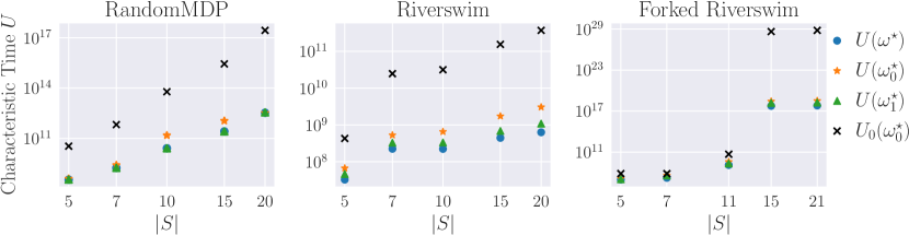
Figure 1: Comparison of the upper bounds (2) and (3) for different sizes of $S$ and $\gamma=0.95$. We evaluated different allocations using $U_{0}(\omega)$ and $U(\omega)$. The allocations are: $\omega_{0}^{\star}$ (the optimal allocation in (2), $\omega^{\star}$ (the optimal allocation in (3) and $\omega_{1}^{\star}$ (the optimal allocation in (4) by setting $k=1$ uniformly across states and actions). For the random MDP we show the median value across $30$ runs.

4.2 Example on Tabular MDPs

In Figure 1, we compare the characteristic time upper bounds obtained in the previous subsection. These upper bounds correspond to the allocations $\omega^{\star}$, $\omega_{0}^{\star}$, and $\omega_{1}^{\star}$ obtained by minimizing, over $\Delta(S\times A)$, $U(\omega)$, $U_{0}(\omega)$, and $U_{1}(\omega)$, respectively. We evaluated these characteristic times on various MDPs: (1) a random MDP (see Appendix A ); (2) the RiverSwim environment [60]; (3) the Forked RiverSwim, a novel environment where the agent needs to constantly explore two different states to learn the optimal policy (compared to the RiverSwim environment, the sample complexity is higher; refer to Appendix A for a complete description).

We note that across all plots, the optimal allocation $\omega_{0}^{\star}$ has a quite large characteristic time (black cross). Instead, the optimal allocation $\omega^{\star}$ (blue circle) computed using our new upper bound (3) achieves a lower characteristic time. When we evaluate $\omega_{0}^{\star}$ on the new bound (3) (orange star), we observe similar characteristic times.

Finally, to verify that we can indeed choose $k=1$ uniformly across states and actions, we evaluated the characteristic time $\omega_{1}^{\star}$ computed using (4) (green triangle). Our results indicate that the performance is not different from those obtained with $\omega^{\star}$, suggesting that the quantities of interest (gaps and variances) are enough to learn an efficient exploration allocation. We investigate the choice of $k$ in more detail in Appendix A .

5 Model-Free Active Exploration Algorithms

In this section we present MF-BPI, a model-free exploration algorithm that leverages the optimal allocations obtained through the previously derived upper bound of the sample complexity lower bound. We first present an upper bound $\tilde{U}(\omega)$ of $U(\omega)$, so that it is possible to derive a closed form solution of the optimal allocation (an idea previously proposed in [37]).

Proposition 5.1.

Assume that $\phi$ has a unique optimal policy $\pi^{\star}$. For all $\omega\in\Delta(S\times A)$, we have:

$$U(\omega)\leq\tilde{U}(\omega):=\max_{s,a\neq\pi^{\star}(s)}\frac{H(s,a)}{\omega(s,a)}+\frac{H}{\min_{s^{\prime}}\omega(s^{\prime},\pi^{\star}(s^{\prime}))},$$

with $H(s,a)\coloneqq\frac{2+8\varphi^{2}M_{sa}^{k}[V^{\star}]^{2^{1-k}}}{\Delta(s,a)^{2}}$ and $H\coloneqq\frac{\max_{s^{\prime}}C(s^{\prime})(1+\gamma)^{2}}{\Delta_{\min}^{2}(1-\gamma)^{2}}$. The minimizer $\tilde{\omega}^{\star}\coloneqq\arg\inf_{\omega}\tilde{U}(\omega)$ satisfies $\tilde{\omega}^{\star}(s,a)\propto H(s,a)$ for $a\neq\pi^{\star}(s)$ and $\tilde{\omega}^{\star}(s,\pi^{\star}(s))\propto\sqrt{H\sum_{s,a\neq\pi^{\star}(s)}H(s,a)/|S|}$ otherwise.

In the MF-BPI algorithm, we estimate the gaps $\Delta(s,a)$ and $M_{sa}^{k}[V^{\star}]$ for a fixed small value of $k$ (we later explain how to do this in a model-free manner.) and compute the corresponding allocation $\tilde{\omega}^{\star}$. This allocation drives the exploration under MF-BPI. Using this design approach, we face two issues:

(1) Uniform $k$ and regularization. It is impractical to estimate $M_{sa}^{k}[V^{\star}]$ for multiple values of $k$. Instead, we fix a small value of $k$ (e.g., $k=1$ or $k=2$) for all state-action pairs (refer to the previous section for a discussion on this choice). Then, to avoid excessively small values of the gaps in the denominator, we regularize the allocation $\tilde{\omega}^{\star}$ by replacing, in the expression of $H(s,a)$ (resp. $H_{\min}$), $\Delta(s,a)$ (resp. $\Delta_{\min}$) by $(\Delta(s,a)+\lambda)$ (resp. $(\Delta_{\min}+\lambda)$) for some $\lambda>0$.

(2) Handling parametric uncertainty via bootstrapping. The quantities $\Delta(s,a)$ and $M_{sa}^{k}[V^{\star}]$ required to compute $\tilde{\omega}^{\star}$ remain unknown during training, and we adopt the Certainty Equivalence principle, substituting the current estimates of these quantities to compute the exploration strategy. By doing so, we are inherently introducing parametric uncertainty into these terms that is not taken into account by the allocation $\tilde{\omega}^{\star}$. To deal with this uncertainty, the traditional method, as used e.g. in [37, 38]), involves using $\epsilon$-soft exploration policies to guarantee that all state-action pairs are visited infinitely often. This ensures that the estimation errors vanish as time grows large. In practice, we find this type of forced exploration inefficient. In MF-BPI, we opt for a bootstrapping approach to manage parametric uncertainties, which can augment the traditional forced exploration step, leading to more principled exploration.

5.1 Exploration in tabular MDPs.

Algorithm 1 Boostrapped MF-BPI (Boostrapped Model Free Best Policy Identification)

0:  Parameters $(\lambda,k,p)$; ensemble size $B$; learning rates $\{(\alpha_{t},\beta_{t})\}_{t}$.

1:  Initialize $Q_{1,b}(s,a)\sim{\cal U}([0,1/(1-\gamma)])$ and $M_{1,b}(s,a)\sim{\cal U}([0,1/(1-\gamma)^{2^{k}}])$ for all $(s,a)\in S\times A$ and $b\in[B]$.

2:  for $t=0,1,2,\dots,$ do

3:     Bootstrap a sample $(\hat{Q}_{t},\hat{M}_{t})$ from the ensemble, and compute the allocation $\omega^{(t)}$ using Proposition 5.1. Sample $a_{t}\sim\omega^{(t)}(s_{t},\cdot)$; observe $(r_{t},s_{t+1})\sim q(\cdot|s_{t},a_{t})\otimes P(\cdot|s_{t},a_{t})$.

4:     for $b=1,\dots,B$ do

5:        With probability $p$, using the experience $(s_{t},a_{t},r_{t},s_{t+1})$, update $Q_{t,b}$ and $M_{t,b}$ using Equations 5 and 6.

6:     end for

7:  end for

The pseudo-code of MF-BPI for tabular MDPs is presented in Algorithm 1. In round $t$, MF-BPI explores the MDP using the allocation $\omega^{(t)}$ estimating $\tilde{\omega}^{\star}$. To compute this allocation, we use Proposition 5.1 and need (i) the sub-optimality gaps $\Delta(s,a)$, which can be easily derived from the $Q$-function; (ii) the $2^{k}$-th moment $M_{sa}^{k}[V^{\star}]$, which can always be learnt by means of stochastic approximation. In fact, for any Markovian policy $\pi$ and pair $(s,a)$ we have $M_{sa}^{k}[V_{\phi}^{\pi}]=\frac{1}{\gamma^{2^{k}}}\mathbb{E}_{s^{\prime}\sim P(\cdot|s,a)}[\delta^{\pi}(s,a,s^{\prime})^{2^{k}}],$ where $\delta^{\pi}(s,a,s^{\prime})=r(s,a)+\gamma\mathbb{E}_{a^{\prime}\sim\pi(\cdot|s^{\prime})}[Q^{\pi}(s^{\prime},a^{\prime})]-Q^{\pi}(s,a)$ is a variant of the TD-error. MF-BPI then uses an asynchronous two-timescale stochastic approximation algorithm to learn $Q^{\star}$ and $M_{sa}^{k}[V^{\star}]$,

$$Q_{t+1}(s_{t},a_{t}) =Q_{t}(s_{t},a_{t})+\alpha_{t}(s_{t},a_{t})\left(r_{t}+\gamma\max_{a}Q_{t}(s_{t+1},a)-Q_{t}(s_{t},a_{t})\right),$$ (5)

$$M_{t+1}(s_{t},a_{t}) =M_{t}(s_{t},a_{t})+\beta_{t}(s_{t},a_{t})\left(\left(\delta_{t}^{\prime}/\gamma\right)^{2^{k}}-M_{t}(s_{t},a_{t})\right),$$ (6)

where $\delta_{t}^{\prime}=r_{t}+\gamma\max_{a}Q_{t+1}(s_{t+1},a)-Q_{t+1}(s_{t},a_{t})$, and $\{(\alpha_{t},\beta_{t})\}_{t\geq 0}$ are learning rates satisfying $\sum_{t\geq 0}\alpha_{t}(s,a)=\sum_{t\geq 0}\beta_{t}(s,a)=\infty,\sum_{t\geq 0}(\alpha_{t}(s,a)^{2}+\beta_{t}(s,a)^{2})\leq\infty$, and $\frac{\alpha_{t}(s,a)}{\beta_{t}(s,a)}\to 0$.

MF-BPI uses bootstrapping to handle parametric uncertainty. We maintain an ensemble of $(Q,M)$-values, with $B$ members, from which we sample $(\hat{Q}_{t},\hat{M}_{t})$ at time $t$. This sample is generated by sampling a uniform random variable $\xi\sim{\cal U}([0,1])$ and, for each $(s,a)$ set $\hat{Q}_{t}(s,a)={\rm Quantile}_{\xi}({Q_{t,1}(s,a),\dots,Q_{t,B}(s,a)})$ (assuming a linear interpolation). This method is akin to sampling from the parametric uncertainty distribution (we perform the same operation also to compute $\hat{M}_{t}$). This sample is used to compute the allocation $\omega^{(t)}$ using Proposition 5.1 by setting $\Delta_{t}(s,a)=\max_{a^{\prime}}\hat{Q}_{t}(s,a^{\prime})-\hat{Q}_{t}(s,a)$, $\pi_{t}^{\star}(s)=\operatorname*{arg\,max}_{a}\hat{Q}_{t}(s,a)$ and ${\Delta}_{\textrm{min},t}=\min_{s,a\neq\pi_{t}^{\star}(s)}\Delta_{t}(s,a)$. Note that, the allocation $\omega^{(t)}$ can be mixed with a uniform policy, to guarantee asymptotic convergence of the estimates. Upon observing an experience, with probability $p$, MF-BPI updates a member of the ensemble using this new experience. $p$ tunes the rate at which the models are updated, similar to sampling with replacement, speeding up the learning process. Selecting a high value for $p$ compromises the estimation of the parametric uncertainty, whereas choosing a low value may slow down the learning process.

Exploration without bootstrapping? To illustrate the need for our bootstrapping approach, we tried to use the allocation $\omega^{(t)}$ mixed with a uniform allocation. In Figure 2, we show the results on Riverswim-like environments with $5$ states. While forced exploration ensures infinite visits to all state-action pairs, this guarantee only holds asymptotically. As a result, the allocation mainly focuses on the current MDP estimate, neglecting other plausible MDPs that could produce the same data. This makes the forced exploration approach too sluggish for effective convergence, suggesting its inadequacy for rapid policy learning. These results highlight the need to account for the uncertainty in $Q,M$ when computing the allocation.

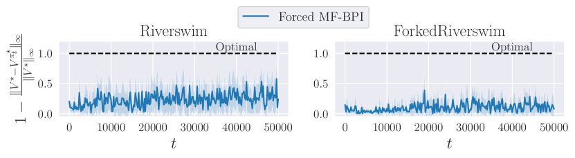
Figure 2: Forced exploration example with $5$ states. We explore according to $\omega^{(t)}(s_{t},a)=(1-\epsilon_{t})\frac{\tilde{\omega}_{t}^{\star}(s_{t},a)}{\sum_{a^{\prime}}\tilde{\omega}_{t}^{\star}(s_{t},a^{\prime})}+\epsilon_{t}\frac{1}{|A|}$, mixing the estimate of the allocation $\tilde{\omega}^{\star}$ from Proposition 5.1 with a uniform policy, with $\epsilon_{t}=\max(10^{-3},1/N_{t}(s_{t}))$ where $N_{t}(s)$ indicates the number of times the agent visited state $s$ up to time $t$. Shade indicates $95\%$ confidence interval.

Algorithm 2 DBMF-BPI (Deep Bootstrapped Model Free BPI)

0:  Parameters $(\lambda,k)$; ensemble size $B$; exploration rate $\{\epsilon_{t}\}_{t}$; estimate ${\Delta}_{\textrm{min},0}$; mask probability $p$.

1:  Initialize replay buffer ${\cal D}$, networks $Q_{\theta_{b}},M_{\tau_{b}}$ and targets $Q_{\theta^{\prime}_{b}}$ for all $b\in[B]$.

2:  for $t=0,1,2,\dots,$ do

3:    Sampling step.

4:       Compute allocation $\omega^{(t)}\leftarrow{\tt ComputeAllocation}(s_{t},\{Q_{\theta_{b}},M_{\tau_{b}}\}_{b\in[B]},{\Delta}_{\textrm{min},t},\gamma,\lambda,k,\epsilon_{t})$.

5:       Sample $a_{t}\sim\omega^{(t)}(s_{t},\cdot)$ and observe $(r_{t},s_{t+1})\sim q(\cdot|s_{t},a_{t})\otimes P(\cdot|s_{t},a_{t})$.

6:       Add transition $z_{t}=(s_{t},a_{t},r_{t},s_{t+1})$ to the replay buffer ${\cal D}$.

7:    Training step.

8:       Sample a batch ${\cal B}$ from ${\cal D}$, and with probability $p$ add the $i^{th}$ experience in ${\cal B}$ to a sub-batch ${\cal B}_{b}$, $\forall b\in[B]$. Update the $(Q,M)$-values of the $b^{th}$ member in the ensemble using ${\cal B}_{b}$: $\{Q_{\theta_{b}},Q_{\theta_{b}^{\prime}},M_{\tau_{b}}\}_{b\in[B]}\leftarrow{\tt Training}(\{{\cal B}_{b},Q_{\theta_{b}},Q_{\theta_{b}^{\prime}},M_{\tau_{b}}\}_{b\in[B]})$.

9:       Update estimate ${\Delta}_{\textrm{min},t+1}\leftarrow{\tt EstimateMinimumGap}({\Delta}_{\textrm{min},t},{\cal B},\{Q_{\theta_{b}}\}_{b\in[B]})$.

10:  end for

5.2 Extension to Deep Reinforcement Learning

To extend bootstrapped MF-BPI to continuous MDPs, we propose DBMF-BPI (see Algorithm 2, or Appendix B ). DBMF-BPI uses the mechanism of prior networks from BSP [50](bootstrapping with additive prior) to account for uncertainty that does not originate from the observed data. As before, we keep an ensemble $\{Q_{\theta_{1}},\dots,Q_{\theta_{B}}\}$ of $Q$-values (with their target networks) and an ensemble $\{M_{\tau_{1}},\dots,M_{\tau_{B}}\}$ of $M$-values, as well as their prior networks. We use the same procedure as in the tabular case to compute $(\hat{Q}_{t},\hat{M}_{t})$ at time $t$, except that we sample $\xi\sim{\cal U}([0,1])$ every $T_{s}\propto(1-\gamma)^{-1}$ training steps (or at the end of an episode) to make the training procedure more stable. The quantity $\hat{Q}_{t}$ is used to compute $\pi_{t}^{\star}(s_{t})$ and $\Delta_{t}(s_{t},a)$. We estimate ${\Delta}_{\textrm{min},t}$ via stochastic approximation, with the minimum gap from the last batch of transitions sampled from the replay buffer serving as a target. To derive the exploration strategy, we compute $H_{t}(s_{t},a)=\frac{2+8\varphi^{2}\hat{M}_{t}(s_{t},a)^{2^{1-k}}}{(\Delta_{t}(s_{t},a)+\lambda)^{2}}$ and $H_{t}=\frac{4(1+\gamma)^{2}\max(1,4\gamma^{2}\varphi^{2}\hat{M}_{t}(s_{t},\pi_{t}^{\star}(s_{t}))^{2^{1-k}})}{({\Delta}_{\textrm{min},t}+\lambda)^{2}(1-\gamma)^{2}}$. Next, we set the allocation $\omega_{o}^{(t)}$ as follows: $\omega_{o}^{(t)}(s_{t},a)=H_{t}(s_{t},a)$ if $a\neq\pi_{t}^{\star}(s_{t})$ and $\omega_{o}^{(t)}(s_{t},a)=\sqrt{H_{t}\sum_{a\neq\pi_{t}^{\star}(s_{t})}H_{t}(s_{t},a)}$ otherwise. Finally, we obtain an $\epsilon_{t}$-soft exploration policy $\omega^{(t)}(s_{t},\cdot)$ by mixing $\omega_{o}^{(t)}(s_{t},\cdot)/\sum_{a}\omega_{o}^{(t)}(s_{t},a)$ with a uniform distribution (using an exploration parameter $\epsilon_{t}$).

6 Numerical Results

We evaluate the performance of MF-BPI on benchmark problems and compare it against state-of-the-art methods (details can be found in Appendix A ).

Tabular MDPs. In the tabular case, we compared various algorithms on the Riverswim and Forked Riverswim environments. We evaluate MF-BPI with (1) bootstrapping and with (2) the forced exploration step using an $\epsilon$-soft exploration policy, MDP-NaS [38], PSRL [47] and Q-UCB [28, 71]. For MDP-NaS, the model of the MDP was initialized in an optimistic way (with additive smoothing). In both environments, we varied the size of the state space. In Figure 3, we show $1-\frac{\|V^{\star}-V^{\pi_{T}^{\star}}\|_{\infty}}{\|V^{\star}\|_{\infty}}$, a performance measure for the estimated policy $\pi_{T}^{\star}$ after $T=|S|\times 10^{4}$ steps with $\gamma=0.99$. Results (the higher the better) indicate that bootstrapped MF-BPI can compete with model-based and model-free algorithms on hard-exploration problems, without resorting to expensive model-based procedures. Details of the experiments, including the initialization of the algorithms, are provided in Appendix A .

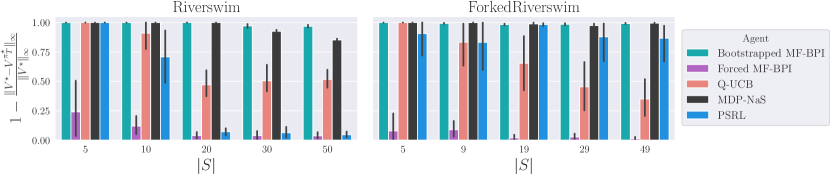
Figure 3: Evaluation of the estimated optimal policy $\pi_{T}^{\star}$ after $T$ steps for MF-BPI, Q-UCB, MDP-NaS and PSRL. Results are averaged across 10 seeds and lines indicate $95\%$ confidence intervals.

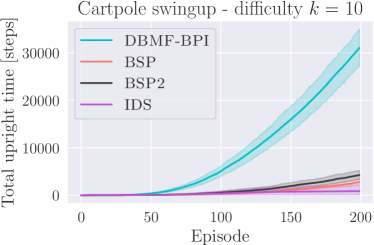
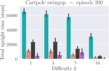
Figure 4: Cartpole swingup problem. On the left: total upright time at a difficulty level of $k=10$. On the right: total upright time after $200$ episodes for different difficulties $k$. To observe a positive reward, the pole’s angle must satisfy $\cos(\theta)>k/20$, and the cart’s position should satisfy $|x|\leq 1-k/20$. Bars and shaded areas indicate $95\%$ confidence intervals.

Deep RL. In environments with continuous state space, we compared DBMF-BPI with BSP [51, 50] (Bootstrapped DQN with randomized priors) and IDS [44] (Information-Directed Sampling). We also evaluated DBMF-BPI against BSP2, a variant of BSP that uses the same masking mechanism as DBMF-BPI for updating the ensemble. These methods were tested on challenging exploration problems from the DeepMind behavior suite [52] with varying levels of difficulty: (1) a stochastic version of DeepSea and (2) the Cartpole swingup problem. The DeepSea problem includes a $5\%$ probability of the agent slipping, i.e., that an incorrect action is executed, which increases the aleatoric variance.

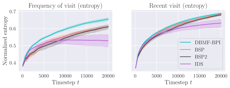
Figure 5: Exploration in Cartpole swingup for $k=5$. On the left, we show the entropy of visitation frequency for the state space $(x,\dot{x},\theta,\dot{\theta})$ during training. On the right, we show a measure of the dispersion of the most recent visits; smaller values indicate that the agent is less explorative as $t$ increases.

The results for the Cartpole swingup problem are depicted in Figure 4 for various difficulty levels $k$ (see also Section A.5 for more details), demonstrating the ability of DBMF-BPI to quickly learn an efficient policy. While BSP generally performs well, there is a notable difference in performance when compared to DBMF-BPI. For a fair comparison, we used the same network initialization across all methods, except for IDS. Untuned, IDS performed poorly; proper initialization improved its performance, but results remained unsatisfactory. In Figure 5, we present two exploration metrics for difficulty $k=5$. The frequency of visits measures the uniformity and dispersion of visits across the state space, while the second metric evaluates the recency of visits to different regions, capturing how frequently the methods keep visiting previously visited states (a smaller value indicates that the agent tends to concentrate on a specific region of the state space). For detailed analysis, please refer to appendix A.

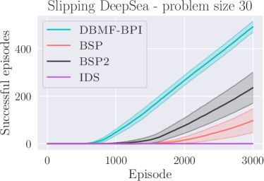
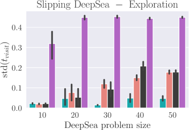
Figure 6: Slipping DeepSea problem. On the left: total number of successful episodes (i.e., that the agent managed to reach the final reward) for a grid with $30^{2}$ input features. On the right: standard deviation of $t_{{\rm visit}}$ at the last episode, depicting how much each agent explored (the lower the better).

For the slipping DeepSea problem, results are depicted in Fig. 6 (see also Section A.4 for more details). Besides the number of successful episodes, we also display the standard deviation of $(t_{{\rm visit}})_{ij}$ across all cells $(i,j)$, where $(t_{{\rm visit}})_{ij}$ indicates the last timestep $t$ that a cell $(i,j)$ was visited (normalized by $NT$, the product of the grid size, and the number of episodes). The right plot shows $\mathrm{std}(t_{{\rm visit}})$ for different problem sizes, highlighting the good exploration properties of DBMF-BPI. Additional details and exploration metrics can be found in Appendix A .

7 Conclusions

In this work, we studied the problem of exploration in Reinforcement Learning and presented MF-BPI, a model-free solution for both tabular and continuous state-space MDPs. To derive this method, we established a novel approximation of the instance-specific lower bound necessary for identifying nearly-optimal policies. Importantly, this approximation depends only on quantities learnable via stochastic approximation, paving the way towards model-free methods. Numerical results on hard-exploration problems highlighted the effectiveness of our approach for learning efficient policies over state-of-the-art methods.

Appendix

Contents

1. 1 Introduction
2. 2 Related Work
3. 3 Preliminaries
4. 4 Towards Efficient Exploration Allocations
   1. 4.1 Upper bounds on $T_{\varepsilon}(\omega)$
   2. 4.2 Example on Tabular MDPs
5. 5 Model-Free Active Exploration Algorithms
   1. 5.1 Exploration in tabular MDPs.
   2. 5.2 Extension to Deep Reinforcement Learning
6. 6 Numerical Results
7. 7 Conclusions
8. A Numerical Results
   1. A.1 The Forked Riverswim Environment
   2. A.2 Details of Example 4.2
   3. A.3 Riverswim and Forked Riverswim - Description and Additional Results
   4. A.4 Slipping DeepSea - Description and Additional Results
   5. A.5 Cartpole Swingup - Description and Additional Results
   6. A.6 Parameters, Hardware, Code and Libraries
      1. A.6.1 Simulation parameters - Riverswim and Forked Riverswim
      2. A.6.2 Simulation parameters - Slipping DeepSea
      3. A.6.3 Simulation parameters - Cartpole Swingup
      4. A.6.4 Hardware and simulation time
      5. A.6.5 Code and libraries
9. B Algorithms
   1. B.1 PS-MDP-NaS - Posterior Sampling for navigating MDPs
   2. B.2 O-BPI - Online Best Policy Identification
   3. B.3 Boostrapped MF-BPI - Model Free Best Policy Identification
   4. B.4 DBMF-BPI - Deep Boostrapped Model Free Best Policy Identification
10. C Proofs
    1. C.1 Preliminaries
    2. C.2 Alternative upper bounds
       1. C.2.1 Sample complexity lower bound
       2. C.2.2 Upper bound on $T_{\varepsilon}(\omega)$
       3. C.2.3 Closed form solution under the generative model
       4. C.2.4 Technical lemmas
       5. C.2.5 Decomposition of the set of confusing MDPs

Appendix introduction

We start by examining the wider impact of our work and acknowledging its limitations. This provides a balanced view of our contribution and points out areas for future research.

Next, we turn to the numerical results. Here, we give a more detailed account of our findings and include additional results for further clarity. We also introduce and describe the new Forked RiverSwim environment, an advanced version of the existing RiverSwim model, which has a larger sample complexity.

In the subsequent section, we break down the algorithms used in our study. This gives a deeper understanding of the methods underpinning our research.

We wrap up the appendix by providing all the proofs that support our conclusions.

Broader impact

This paper primarily focuses on foundational research in reinforcement learning, specifically the exploration problem, and proposes a novel model-free exploration strategy. While our work does not directly engage with societal impact considerations, we acknowledge the importance of considering the broader implications of AI technologies. As our proposed method improves the efficiency of reinforcement learning algorithms, it could potentially be applied in a wide range of contexts, some of which could have societal impacts. For instance, reinforcement learning is used in decision-making systems, which could include areas like healthcare, finance, and autonomous vehicles, where biases or errors could have significant consequences. Hence, while the direct societal impact of our work may not be immediately apparent, we strongly encourage future researchers and practitioners who apply these techniques to carefully consider the ethical implications and potential negative impacts in their specific use-cases. The responsible use of AI, including the mitigation of bias and the respect for privacy, should always be a priority.

Limitations

While our work presents significant advancements in the area of reinforcement learning, it also has its limitations that need to be acknowledged:

• Assumptions: Our approach relies on the assumption that the MDP is communicating. The instance-specific lower bound we propose may not be as effective if this assumption does not hold.

• Scalability: Our method, despite being model-free, still relies on stochastic approximations, which may not scale well with the complexity and size of certain MDPs.

• Comparison with Model-Based Approaches: While we have shown that our approach performs competitively with existing model-based exploration algorithms in hard-exploration environments, a comprehensive comparison across a wider range of environments is needed. It is possible that our method may not perform as well in some MDPs as the model-based approaches.

• Bootstrapping: Although bootstrapping has proven to be an effective technique, its usage is yet to be fully understood in RL applications. To achieve a more profound theoretical comprehension, a comprehensive analysis is necessary.

These limitations present opportunities for future research and the continued evolution of efficient exploration in reinforcement learning.

Appendix A Numerical Results

The appendix begins with the numerical results. We first introduce the Forked RiverSwim environment, a more complex variant of the traditional RiverSwim model.

Our discussion continues with a detailed exposition of Section 4.2, providing further experimental details. We conclude this section with additional findings related to both the tabular case and two specific problems: the CartPole Swing-Up and the Slipping DeepSea.

A.1 The Forked Riverswim Environment

The Forked RiverSwim$(N)$ is a novel environment (see also Figure 7) where the agent needs to constantly explore two different states, $(s_{g},s_{g}^{\prime})$, to learn the optimal policy. The number of states is $2N-1$, and there are $3$ actions.

The environment is similar to RiverSwim, but the initial state $s_{1}$ forks into two rivers: the final state in both branches of the rivers ($s_{g}$ and $s_{g}^{\prime}$) have a similar high reward. Furthermore, the agent can deterministically switch between the two branches at any intermediate state. Intermediate states do not give any reward. Moreover, a little subtlety is that the agent can exploit the deterministic transition between $s_{1}$ and $s_{2}^{\prime}$ to deterministically transition to $s_{2}$ (although this has a small effect as $N$ grows large).

Lastly, the Bernoulli rewards in $s_{g}$ and $s_{g}^{\prime}$, which are the highly rewarding states, are quite similar ($1$ vs $0.95$). Therefore, an optimal policy that starts in $s_{1}$ should achieve a slightly better reward than the optimal policy on the RiverSwim environment with $N+1$ states (due to the fact that the transition to $s_{2}$ from $s_{1}$ can be made in a deterministic way).

Due to these reasons, this variant introduces additional complexity into the decision-making process. It is reasonable that a learning algorithm may learn an approximately good greedy policy in a short time-span, but not exactly the optimal one. In fact, we may expect an algorithm to take longer (compared to Riverswim) to learn the true optimal policy. Finally, always compared to RiverSwim, the sample complexity is of orders of magnitude higher, as also depicted in Figure 1. For a Python implementation, please refer to the GitHub repository of this manuscript.

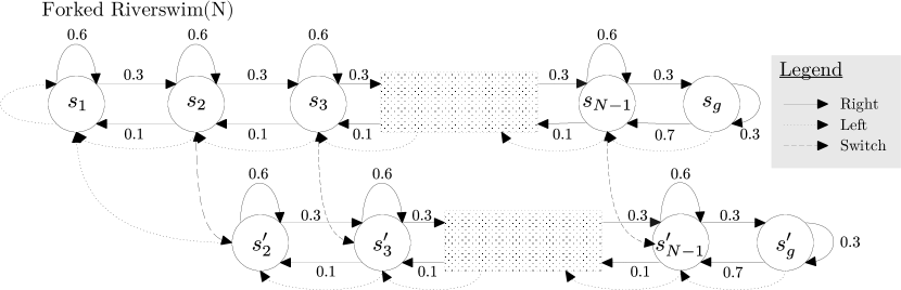
Figure 7: Forked Riverswim$(N)$ with $|S|=2N-1$ states. When taking action left in $s_{1}$ the agent observes a Bernoulli reward $r$ of parameter $0.05$. When taking action right in $s_{g}$ (resp. $s_{g}^{\prime}$) the agent observes a reward $r$ drawn from a Bernoulli of parameter $1$ (resp. $0.95$). In all other states the reward is $0$. Action left and switch are deterministic, while the probability of action Right is indicated in the figure. The square boxes indicate that the pattern of states is being repeated from $s_{3}$ (or $s_{3}^{\prime}$) until $s_{N-1}$ (or $s_{N-1}^{\prime}$). This variant introduces additional complexity into the decision-making process, as the Bernoulli rewards in $s_{g}$ and $s_{g}^{\prime}$ are quite similar ($1$ vs $0.95$).

A.2 Details of Example 4.2

In the following we report the details of Section 4.2. In Section 4.2 we evaluated the characteristic time of three different environments with same discount factor $\gamma=0.95$:

1. RandomMDP: an MDP with $|S|$ states and $3$ actions. The transition probability for each $(s,a)$ is drawn from a Dirichlet distribution ${\rm Dir}(\alpha_{1},\dots,\alpha_{|S|})$, with $\alpha_{i}=\alpha_{i-1}+(i-1)/10$ and $\alpha_{1}=1$. The rewards also follow the same Dirichlet distribution, that is, for each $(s,a)$ we sample a $|S|$-dimensional vector $q$ of rewards from ${\rm Dir}(\alpha_{1},\dots,\alpha_{|S|})$. This vector defines the rewards in the next state $r(s,a,s^{\prime})=q_{s^{\prime}}$, with $q\sim{\rm Dir}(\alpha_{1},\dots,\alpha_{|S|})$. For this type of environment see also the details of the instance-specific quantities in Table 1.

2. RiverSwim: this environment is specified in [60], but we refer to the version used in [38] for a direct comparison. The reward is always $0$ except in the initial state $s_{1}$, and the final state $s_{|S|}$. In the initial state we have $q(1|s_{1},\textrm{left})=0.05$ (probability $0.05$ of observing a reward of $1$, and $0.95$ probability of observing a reward of $0$), while in the final state $q(1|s_{|S|},\textrm{right})=1$. All other rewards are set to $0$. Transition probabilities are the same as in [60]. For this type of environment see also the details of the instance-specific quantities in Table 2.

3. Forked RiverSwim: we refer the reader to Section A.1 for a description of this environment. For this type of environment see also the details of the instance-specific quantities in Table 3.

Interestingly, these environments have different properties that make them suitable for analysis: (1) the RandomMDP environment has very small gaps and variances; (2) the Riverswim environment has a relatively larger maximum span; (3) the Forked Riverswim environment, in contrast to the Riverswim environment, has a very small minimum gap $\Delta_{\min}$ and similar values for the span.

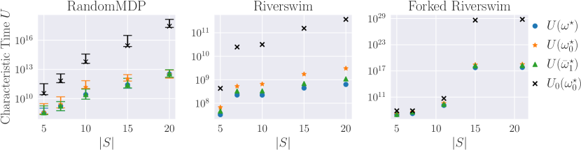
Figure 8: Comparison of (2) and (3) for discount $\gamma=0.99$ and different sizes of the state space $S$. We evaluated different allocations using $U_{0}(\omega)$ and $U(\omega)$. The allocations are: $\omega^{\star}$ (the optimal allocation in Equation 3), $\omega_{0}^{\star}$ (the optimal allocation in Equation 2) and $\omega_{1}^{\star}$ (the optimal allocation that we get from (3) by setting $k=1$ uniformly across states and actions). Results for the RandomMDP indicate the median and the bars 95% confidence intervals across 30 runs.

$|S|$	$\Delta_{\min}$	$\max_{sa}\Delta_{sa}$	$\min_{sa}\operatorname{MD}_{sa}[V^{\star}]$	$\max_{sa}\operatorname{MD}_{sa}[V^{\star}]$	$\min_{sa}\operatorname{Var}_{sa}[V^{\star}]$	$\max_{sa}\operatorname{Var}_{sa}[V^{\star}]$	$\max_{s,a,k}M_{sa}^{k}[V^{\star}]^{2^{-k}}$
$5$	$1.1\cdot 10^{-2}$	$1.6\cdot 10^{-1}$	$6.4\cdot 10^{-2}$	$1.0\cdot 10^{-1}$	$8.3\cdot 10^{-4}$	$3.4\cdot 10^{-3}$	$1.0\cdot 10^{-1}$
$10$	$2.3\cdot 10^{-3}$	$6.3\cdot 10^{-2}$	$2.7\cdot 10^{-2}$	$3.6\cdot 10^{-2}$	$1.4\cdot 10^{-4}$	$3.7\cdot 10^{-4}$	$3.6\cdot 10^{-2}$
$25$	$1.2\cdot 10^{-4}$	$1.0\cdot 10^{-2}$	$4.6\cdot 10^{-3}$	$5.1\cdot 10^{-3}$	$3.3\cdot 10^{-6}$	$4.9\cdot 10^{-6}$	$5.1\cdot 10^{-3}$
$50$	$9.5\cdot 10^{-6}$	$1.9\cdot 10^{-3}$	$9.1\cdot 10^{-4}$	$9.5\cdot 10^{-4}$	$1.2\cdot 10^{-7}$	$1.4\cdot 10^{-7}$	$9.5\cdot 10^{-4}$
$100$	$1.1\cdot 10^{-6}$	$3.7\cdot 10^{-4}$	$1.8\cdot 10^{-4}$	$1.8\cdot 10^{-4}$	$0$	$0$	$1.8\cdot 10^{-4}$

Table 1: Details of the instance-specific quantities for the RandomMDP environment (we evaluated up to $k=19$). Results indicate an average over 300 different realizations. Confidence intervals are omitted for brevity, and values are rounded up to the 1st decimal.

$|S|$	$\Delta_{\min}$	$\max_{sa}\Delta_{sa}$	$\min_{sa}\operatorname{MD}_{sa}[V^{\star}]$	$\max_{sa}\operatorname{MD}_{sa}[V^{\star}]$	$\min_{sa}\operatorname{Var}_{sa}[V^{\star}]$	$\max_{sa}\operatorname{Var}_{sa}[V^{\star}]$	$\max_{s,a,k}M_{sa}^{k}[V^{\star}]^{2^{-k}}$
$5$	$7.6\cdot 10^{-2}$	$1.3\cdot 10^{0}$	$1.7\cdot 10^{0}$	$3.0\cdot 10^{0}$	$0$	$3.6\cdot 10^{-1}$	$1.1\cdot 10^{0}$
$10$	$3.4\cdot 10^{-2}$	$1.3\cdot 10^{0}$	$2.5\cdot 10^{0}$	$4.5\cdot 10^{0}$	$0$	$3.7\cdot 10^{-1}$	$1.1\cdot 10^{0}$
$25$	$1.9\cdot 10^{-2}$	$1.3\cdot 10^{0}$	$2.5\cdot 10^{0}$	$5.0\cdot 10^{0}$	$0$	$3.7\cdot 10^{-1}$	$1.1\cdot 10^{0}$
$50$	$8.4\cdot 10^{-3}$	$1.3\cdot 10^{0}$	$2.7\cdot 10^{0}$	$5.4\cdot 10^{0}$	$0$	$3.7\cdot 10^{-1}$	$1.1\cdot 10^{0}$
$100$	$2.1\cdot 10^{-4}$	$1.3\cdot 10^{0}$	$2.9\cdot 10^{0}$	$5.5\cdot 10^{0}$	$0$	$3.7\cdot 10^{-1}$	$1.1\cdot 10^{0}$

Table 2: Details of the instance-specific quantities for the Riverswim environment (we evaluated up to $k=19$). Values are rounded up to the 1st decimal.

$|S|$	$\Delta_{\min}$	$\max_{sa}\Delta_{sa}$	$\min_{sa}\operatorname{MD}_{sa}[V^{\star}]$	$\max_{sa}\operatorname{MD}_{sa}[V^{\star}]$	$\min_{sa}\operatorname{Var}_{sa}[V^{\star}]$	$\max_{sa}\operatorname{Var}_{sa}[V^{\star}]$	$\max_{s,a,k}M_{sa}^{k}[V^{\star}]^{2^{-k}}$
$5$	$1.0\cdot 10^{-1}$	$1.4\cdot 10^{0}$	$1.0\cdot 10^{0}$	$2.0\cdot 10^{0}$	$0$	$3.2\cdot 10^{-1}$	$1.0\cdot 10^{0}$
$11$	$2.8\cdot 10^{-2}$	$1.3\cdot 10^{0}$	$1.6\cdot 10^{0}$	$2.9\cdot 10^{0}$	$0$	$4.9\cdot 10^{-1}$	$2.0\cdot 10^{0}$
$25$	$1.0\cdot 10^{-6}$	$1.3\cdot 10^{0}$	$1.7\cdot 10^{0}$	$3.2\cdot 10^{0}$	$0$	$4.8\cdot 10^{-1}$	$2.0\cdot 10^{0}$
$51$	$1.0\cdot 10^{-6}$	$1.3\cdot 10^{0}$	$2.1\cdot 10^{0}$	$4.2\cdot 10^{0}$	$0$	$4.8\cdot 10^{-1}$	$2.0\cdot 10^{0}$
$101$	$1.0\cdot 10^{-6}$	$1.3\cdot 10^{0}$	$2.5\cdot 10^{0}$	$5.1\cdot 10^{0}$	$0$	$4.8\cdot 10^{-1}$	$2.0\cdot 10^{0}$

Table 3: Details of the instance-specific quantities for the Forked Riverswim environment (we evaluated up to $k=19$). Values are rounded up to the 1st decimal.

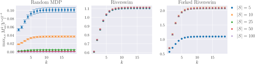
Figure 9: Plot of $\max_{s,a}M_{sa}^{k}[V^{\star}]^{2^{-k}}$ for various values of $k$. For the random MDP we depict the median value, as well as the $95\%$ confidence interval.

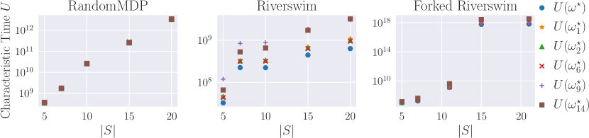
Figure 10: Evaluation of $\omega_{k}^{\star}$ for different values of $k$. For the RandomMDP we only show the median value over $300$ runs.

Finally, in Figure 9, we depict $\max_{s,a}M_{sa}^{k}[V^{\star}]^{2^{-k}}$ for different values of $k$, up to $k=19$. For the RandomMDP environment we observe that $\max_{s,a}M_{sa}^{k}[V^{\star}]^{2^{-k}}$ tends to the maximum of the span $\max_{sa}\operatorname{MD}_{sa}[V^{\star}]$, which depends on the size of the state space (as $|S|$ grows larger the span diminishes). For the other two environments, Riverswim and Forked Riverswim, $\max_{s,a}M_{sa}^{k}[V^{\star}]^{2^{-k}}$ does not seem to depend on the size of the state space. Furthermore, we also observe a sudden convergence of this quantity for relatively small values of $k$, followed by a relatively very slow increase.

In Figure 10 are shown the results when we evaluate the allocations $\omega_{k}^{\star}$ for different values of $k$. In general, we do not observe a striking difference between those allocations.

A.3 Riverswim and Forked Riverswim - Description and Additional Results

In Figure 11 we present results from the Riverswim and ForkedRiverswim environments. These results include data from two new algorithms: O-BPI (Online Best Policy Identification) and PS-MDP-NaS (Posterior Sampling for MDP-NaS).

O-BPI is a novel algorithm that draws inspiration from MDP-NaS. However, a distinguishing characteristic is its use of stochastic approximation to determine the $Q$-values and $M$-values. These values, as for MF-BPI, are used to compute the allocation $\omega$ by solving the sample-complexity bound $\inf_{\omega\in\Omega(\phi)}U(\omega)$ with navigation constraints. On the other hand, PS-MDP-NaS is an adaptation of MDP-NaS that uses posterior sampling over the MDP’s model to address the parametric uncertainty. It’s worth noting that both these algorithms, O-BPI and PS-MDP-NaS, are model-based, and a detailed description of these algorithms is available in the following section, see LABEL:algo:obpi and Algorithm 3.

The results in Figure 11 clearly show the superiority of these allocation computing methods compared to other algorithms such as PSRL and Q-UCB.

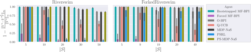
Figure 11: Evaluation of the estimated optimal policy $\pi_{T}^{\star}$ after $T$ steps for MF-BPI, O-BPI, Q-UCB, MDP-NaS, PS-MDP-NaS, and PSRL. Results are averaged across 10 seeds and lines indicate $95\%$ confidence intervals. Note that for Forked Riverswim we have $N=2|S|-1$.

Figure 12 on the next page provides a visualization of the performance of each algorithm over the entire horizon $t=0,\dots,T-1$. We exhibit the performance of the estimated greedy policy $\pi_{t}^{\star}$ at each timestep $t$ for each respective method. The results offer a clear demonstration of the efficiency of those methods based on the instance-specific sample complexity lower bound.

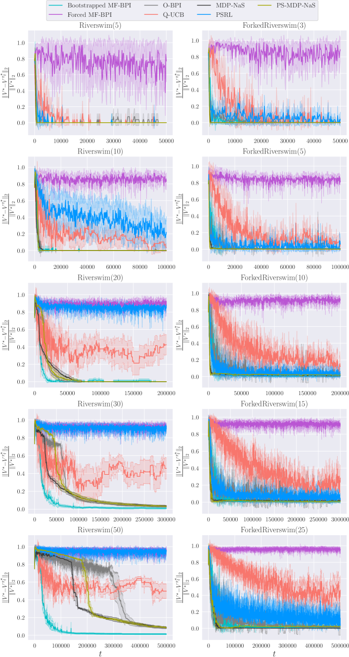
Figure 12: Evaluation of the estimated optimal policy $\pi_{t}^{\star}$ for MF-BPI, O-BPI, Q-UCB, MDP-NaS, PS-MDP-NaS, and PSRL. Results are averaged across 10 seeds and lines indicate $95\%$ confidence intervals.

A.4 Slipping DeepSea - Description and Additional Results

Description.

The Slipping DeepSea problem is an hard-exploration reinforcement learning problem. In the standard version, there’s an $N\times N$ grid, and the agent starts in the top left corner (state 0, 0) and needs to reach the bottom right corner (state $N-1$, $N-1$) for a large reward (the state vector is an $N^{2}$-dimensional vector, that one-hot encodes the agent’s position in the grid). The agent can move diagonally, left or right (or down when close to the wall). The agent incurs in a cost when moving of $0.01/N$, while obtaining a positive reward of $1$ when reaching the bottom right corner. Furthermore, we introduce the modification that there is a small probability of $0.05$ that the incorrect action will be executed. This is a challenging problem because the optimal policy requires the agent to move (incurring a negative reward) many times before eventually reaching the high reward in the bottom right corner. However, due to the stochastic nature of the problem (the chance of slipping), the agent might be forced to take suboptimal actions, making it harder to learn the optimal policy.

Additional results.

Figure 13 presents additional metrics encapsulating the exploration conducted by each algorithm, offering a comprehensive summary of the exploration process after $T$ episodes for each size $N$ (note that for a given size $N$ the number of input features in the state is $N^{2}$).

We focus on two key metrics: (a) $(t_{{\rm visit}})_{ij}$ and (b) $(t_{{\rm avg}})_{ij}$. Here, (a) $(t_{{\rm visit}})_{ij}$ represents the last timestep $t$ at which a cell $(i,j)$ was visited (this value is normalized by $NT$, the multiplication of the grid size and the number of episodes), while (b) $(t{{\rm avg}})_{ij}$ signifies the average frequency with which a cell $(i,j)$ was visited.

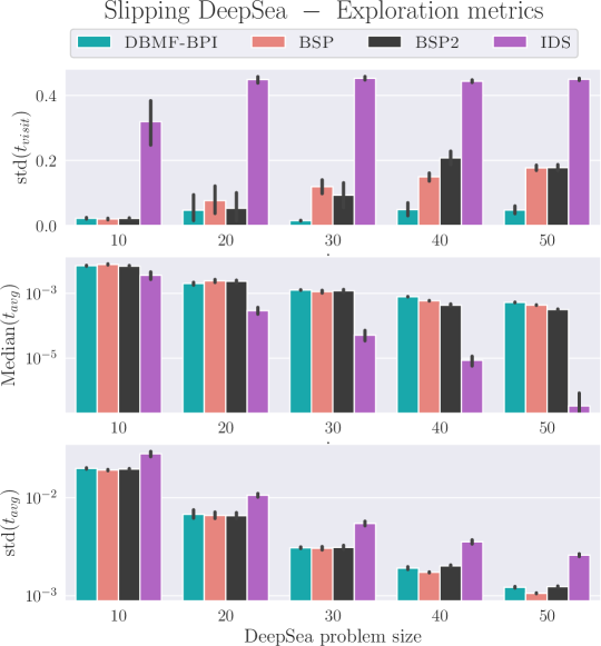
Figure 13: Slipping DeepSea problem - exploration metrics. From top to bottom: (1)standard deviation of $t_{{\rm visit}}$ at the last episode, depicting how much each agent explored (the lower the better); (2) median value of $(t_{{\rm avg}})_{ij}$, i.e., the median value of a cell’s visit frequency; (3) standard deviation of $(t_{{\rm avg}})_{ij}$ across all cells. Results are averaged over $24$ runs and bars indicate $95\%$ confidence intervals.

In terms of arrangement, from the top downwards: (1) we present the standard deviation of $(t_{{\rm visit}})_{ij}$ across all cells; (2) we show the median value of a cell’s visit frequency; (3) we depict the standard deviation of $(t_{{\rm avg}})_{ij}$ across all cells. From the central plot, we notice that DBMF-BPI tends to visit all cells slightly more frequently. The first plot also highlights that DBMF-BPI maintains a consistent visit rate to all cells. This pattern is a strong indication of DBMF-BPI’s explorative behavior. Conversely, neither BSP nor BSP2 match this performance in terms of successful episodes (shown in Figure 14), despite the median value of $t_{{\rm avg}}$ being very similar to that of DBMF-BPI.

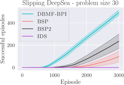
Figure 14: Slipping DeepSea problem. Total number of successful episodes (i.e., that the agent managed to reach the final reward) for a grid with $30^{2}$ input features.

In order to provide a more comprehensive view, Figure 16 and Figure 16 present additional exploration metrics. Specifically, we display $(t_{{\rm avg}})_{ij}$ and $(t_{{\rm visit}})_{ij}$, respectively, after $T=3000$ episodes, given a DeepSea problem size of $30$. The initial plot illustrates how DBMF-BPI tends to concentrate on the grid’s diagonal. However, the bottom plot shows that, in spite of this diagonal focus, DBMF-BPI also maintains a consistent exploration of other cells within the grid. We also observe how BSP seems to uniformly explore all cells, while IDS does not manage to explore the entire grid within the number of episodes.

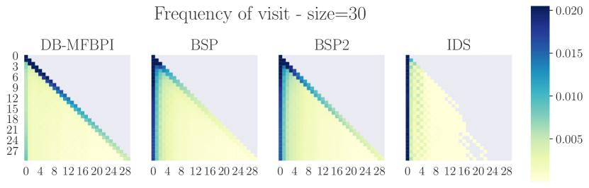
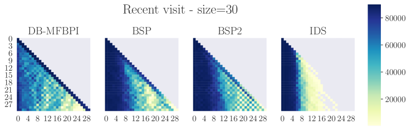
Figure 15: Slipping DeepSea problem. In this figure we depict the average frequency of visits, after $3000$ episodes, when the size of the problem is $k=30$.

Figure 16: Slipping DeepSea problem. In this figure we depict the last timestep a cell was visited, after $3000$ episodes, when the size of the problem is $k=30$.

Last, but not least, on the right column in Figure 17, are shown the results for the learnt greedy policy $\pi_{t}^{\star}$ at time $t$. Clearly, DBMF-BPI is able to learn an efficient policy more quickly than the other methods for different problem sizes.

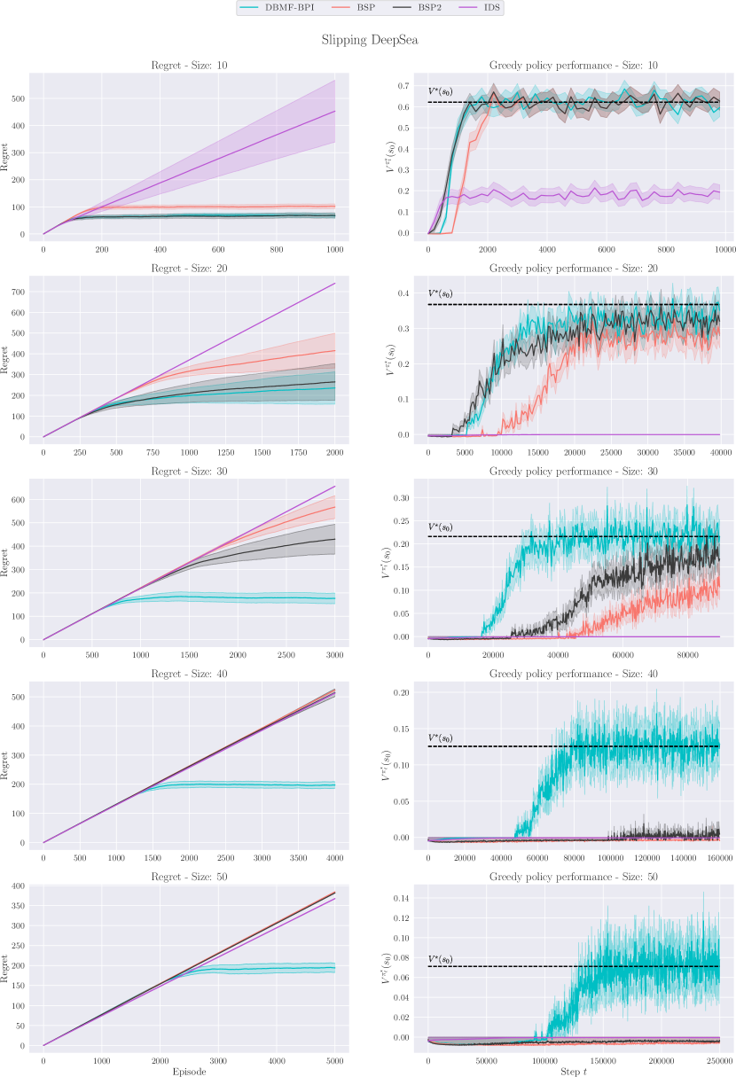
Figure 17: Slipping DeepSea problem - evaluation of the greedy policy. On the left we depict the regret of the learning agent over the number of episodes $T$ for each problem size $k$. On the right, we display the average value of the learnt greedy policy $\pi_{t}^{\star}$ at time $t$ (black dashed-line indicates the average optimal value). Results are averaged over $24$ runs, and the shaded area depicts $95\%$ confidence intervals.

A.5 Cartpole Swingup - Description and Additional Results

Description.

In this subsection we present additional results for the Cartpole swingup problem. The cartpole swingup problem is a classic problem in control theory and reinforcement learning [9]. The task is to balance a pole that is attached by an un-actuated joint to a cart, which moves along a frictionless track. The system is controlled by applying a force to the cart. Initially, the pole is hanging down and the goal is to swing it up so it stays upright. In contrast to the classic cartpole balance problem, the pole needs not only to be balanced when it’s upright but also to be swung up to the upright position.

The state of the system at any point in time is described by four variables: the position of the cart $x$, the velocity of the cart $\dot{x}$, the angle of the pole $\theta$, and the angular velocity of the pole $\dot{\theta}$. There are $4$ additional variables in the state, and for simplicity we refer the user to [52].

To make the problem more difficult, as in [52] we introduce a parameter $k\in\{1,\dots,19\}$ (to not be confused with the parameter of $M_{sa}^{k}[V^{\star}]$) that parameterizes the reward function. Specifically, the agent observes a positive reward of $1$ only if the pole’s angle satisfies $\cos(\theta)>k/20$, and the cart’s position satisfies $|x|\leq 1-k/20$. There is also a negative reward of $-0.1$ that the agent incurs for moving, which aggravates the explore-exploit tradeoff (algorithms like DQN [41] simply remain still).

Additional results.

In Figures 18, 19 and 20, we provide supplementary results for this problem. Figure 18 illustrates the total upright time achieved by each learner after $200$ episodes, across various difficulty levels, $k$. Here, the total upright time refers to the total count of steps where the pole maintained an angle satisfying $\cos(\theta)>k/20$, concurrently with the cart maintaining a position that satisfied $|x|\leq 1-k/20$.

Subsequently, Figure 19 showcases the evolution of this metric throughout all $200$ episodes.

Figure 20 demonstrates the performance of the learnt greedy policy $\pi_{t}^{\star}$ over the course of the training. Every $10$ episodes, we evaluated the greedy policy over $20$ episodes and computed the cumulative reward.

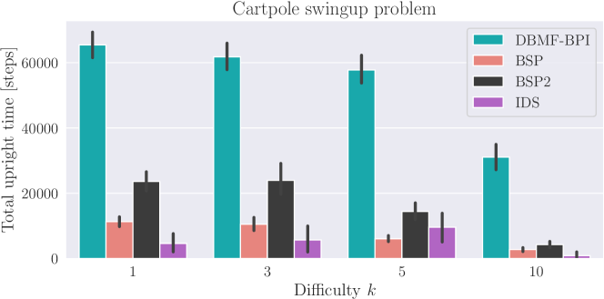
Figure 18: Cartpole swingup problem. Total upright time after $200$ episodes for different difficulties $k$. To observe a positive reward, the pole’s angle must satisfy $\cos(\theta)>k/20$, and the cart’s position should satisfy $|x|\leq 1-k/20$. Bars indicate $95\%$ confidence intervals.

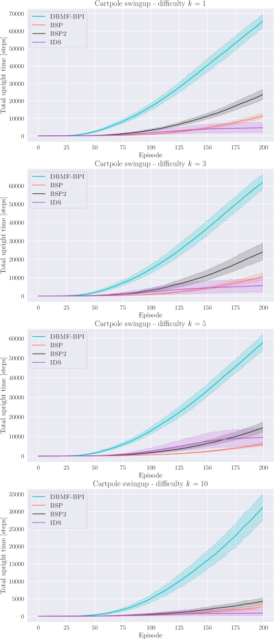
Figure 19: Cartpole swingup problem. Total upright time over $200$ episodes for different difficulties $k$. To observe a positive reward, the pole’s angle must satisfy $\cos(\theta)>k/20$, and the cart’s position should satisfy $|x|\leq 1-k/20$. Bars indicate $95\%$ confidence intervals.

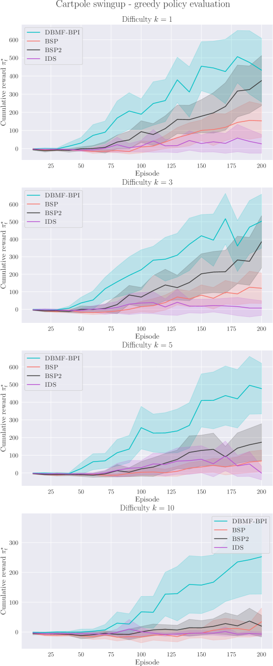
Figure 20: Cartpole swingup problem. Performance of the learnt greedy policy $\pi_{t}^{\star}$ over the training episodes (average cumulative reward collected by the greedy policy).

Exploration results.

In Figures 21, 22 and 23, we show additional results that illustrate the exploration of the various algorithms for difficulties $k=3,5$.

In Figure 21, we display two metrics at each training step $t$: the entropy of visit frequency and the entropy of the most recent visit. The first metric quantifies how thoroughly the method has explored the state space $(x,\dot{x},\theta,\dot{\theta})$ up to time $t$. To do this, we discretize the state space into bins and tally the occurrences in each bin. We then normalize these counts by their sum and calculate the resulting entropy, which is normalized to the range $[0,1]$.

While this measure of visit frequency provides some insight, it is insufficient for understanding whether the algorithm continues to explore new states or revisits old ones. To address this, the second metric measures the dispersion of the timing of the last visits to various regions of the state space. A larger dispersion indicates that the algorithm is concentrating on a specific region, resulting in a smaller entropy (and vice-versa). To calculate this, we again use normalized entropy.

Finally, in Figure 22 and Figure 23, we illustrate the visitation frequency after $20K$ training steps for $(x,\dot{x})$ and $(\dot{x},\dot{\theta})$ at difficulty levels $k=3$ and $k=5$. Darker regions signify higher visitation frequencies. The pattern in $(\dot{x},\dot{\theta})$ is characteristic of algorithms that have learned to stabilize the policy. Notably, DBMF-BPI is also actively exploring various velocities. A similar trend is observed for $(x,\dot{x})$: while most methods focus on an s-shaped trajectory, DBMF-BPI also explores other regions of the state space.

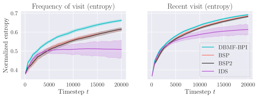
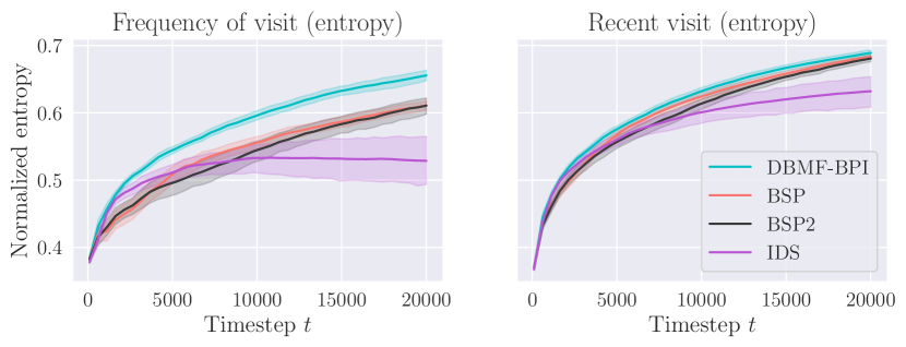
Figure 21: Exploration in Cartpole swingup: At the top, we present results for difficulty $k=3$, and at the bottom, for $k=5$. In the left column, we depict the entropy of visitation frequency for the state space $(x,\dot{x},\theta,\dot{\theta})$ during training. In the right column, we display a measure of the dispersion of the most recent visits; smaller values indicate that the agent is less explorative as $t$ increases.

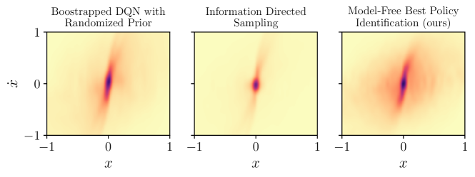
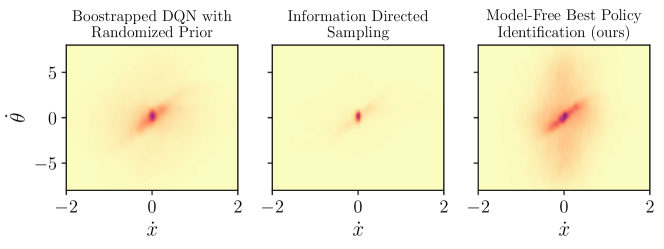
Figure 22: Cartpole Swingup [52] after $20$K training steps for difficulty $k=3$, comparing BSP (Bootstrapped DQN with randomized priors) [50], IDS (Information-Directed Sampling) [44], and MF-BPI (Model-Free Best Policy Identification). Darker areas indicate higher visitation frequency. At the top we show this frequency for $(x,\dot{x})$, the cart’s position and linear’s velocity, and at the bottom of $(\dot{x},\dot{\theta})$, the cart’s linear and pole’s angular velocities.

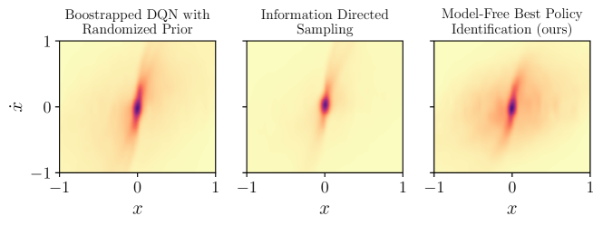
Figure 23: Cartpole Swingup [52] after $20$K training steps for difficulty $k=5$, comparing BSP (Bootstrapped DQN with randomized priors) [50], IDS (Information-Directed Sampling) [44], and MF-BPI (Model-Free Best Policy Identification). Darker areas indicate higher visitation frequency. At the top we show this frequency for $(x,\dot{x})$, the cart’s position and linear’s velocity, and at the bottom of $(\dot{x},\dot{\theta})$, the cart’s linear and pole’s angular velocities.

A.6 Parameters, Hardware, Code and Libraries

In this section, we outline the parameters used for the simulations, describe the hardware employed to run the simulations, and list the libraries that we used.

A.6.1 Simulation parameters - Riverswim and Forked Riverswim

In both the Riverswim and Forked Riverswim environments we used a discount factor of $\gamma=0.99$. Depending on the size of the state space, the horizon length was different. We used $T=10000\times|S|$ for the Riverswim environment, and $T=20000\times N$ for the Forked Riverswim environment (where $N$ is the length of the main river; see also the description of the environment in Section A.1).

We run simulations for $10$ different seeds, and evaluated the estimated greedy policy $\pi_{t}^{\star}$ every $200$ steps. All agents were optimistically initialized (i.e., the $Q$-values were initialized to $1/(1-\gamma)$, etc…), and model-based approaches used additive smoothing (with factor $1$).

For the MDP-NaS and PS-MDP-NaS (see next section for a description) we computed the allocation every $T_{0}=\min(T_{max},\max(200,\frac{T_{max}t}{T/2}))$ steps, where $T_{max}=\frac{2000T}{50000}$. For PSRL we computed a new greedy policy every $\lceil 1/(1-\gamma)\rceil$ steps.

We used a learning rate of $\alpha_{t}=\frac{H+1}{H+k_{t}}$ to learn the $Q$-values, where $H=(1-\gamma)^{-1}$ and $k_{t}=N_{t}(s_{t},a_{t})$ is the number of visits to $(s_{t},a_{t})$ at time $t$. Similarly, to learn the $M$-values we used a learning rate of $\beta_{t}=\alpha_{t}^{1.1}$ (which was not optimized).

For bootstrapped MFBPI we used a parameter $k=1$, and an ensemble size $B=50$ with training probability $p=0.7$. Similarly, these values were not optimized.

All methods that employed an $\epsilon$-soft policy, obtained a final policy $\omega$ by mixing mixed the original policy $\pi$ with a uniform policy as follows $\omega(a|s)=(1-\epsilon_{t})\pi(a|s)+\epsilon_{t}/|A|$. The value of $\epsilon_{t}$ is $\epsilon_{t}=\min(1,1/N_{t}(s_{t}))$ where $N_{t}(s_{t})$ is the total number of visits to state $s_{t}$ at time $t$.

A.6.2 Simulation parameters - Slipping DeepSea

For the DeepSea problem we used a discount factor of $\gamma=0.99$, and different problem sizes $N\in\{10,20,30,40,50\}$. The number of training episodes was $T=100N$. Every $200$ steps we evaluated the performance of the estimated greedy policy $\pi_{t}^{\star}$ over $20$ episodes. For all simulations we used a slipping probability of $0.05$. The number of features in the state is $N^{2}$, and the number of actions is $2$.

Refer to Table 4 for the parameters of the agents.

Table 4: Parameters of the agents for the slipping DeepSea problem.

Property	DBMF-BPI	BSP	BSP 2	IDS
Ensemble size $Q$	$20$	$20$	$20$	$20+\frac{(N-10)}{2}$
Ensemble size $M$	$20$	N.A.	N.A.	N.A.
Hidden layers sizes	$[32]$	$[32]$	$[32]$	$[50]$
Num. of quantiles	N.A.	N.A.	N.A.	$50$
Prior scale $Q$-values
(depends on $N$)	$\{3,5,10,15,20\}$	$\{3,5,10,15,20\}$	$\{3,5,10,15,20\}$	N.A.
Prior scale $M$-values
(depends on $N$)	$\{3,5,10,15,20\}$	$\{3,5,10,15,20\}$	$\{3,5,10,15,20\}$	N.A.
Replay buffer size	$10^{5}$	$10^{5}$	$10^{5}$	$10^{5}$
Training period	$1$	$1$	$1$	$1$
Target network update period	$4$	$4$	$4$	$4$
Batch size	$128$	$128$	$128$	$128$
Mask probability $p$	$0.7$	$0.5$	$0.7$	N.A.
Learning rate $Q$-values	$5\times 10^{-4}$	$10^{-3}$	$10^{-3}$	$5\times 10^{-4}$
Learning rate $M$-values	$5\times 10^{-4}$	N.A.	N.A.	N.A.
Learning rate quantile network	N.A.	N.A.	N.A.	$10^{-6}$
$k$	$2$	N.A.	N.A.	N.A.

A.6.3 Simulation parameters - Cartpole Swingup

For the Cartpole swingup problem we used a discount factor of $\gamma=0.99$, and different difficulties $k\in\{1,3,5,10\}$. The number of training episodes was $T=200$, and we run simulations for $20$ different seeds. Every $10$ steps in the training we evaluated the performance of the estimated greedy policy $\pi_{t}^{\star}$ over $20$ episodes. The state is a vector in $\mathbb{R}^{8}$ and the number of actions is $3$.

For every method, with the exception of IDS, we set up the parameters in the $i^{th}$ layer of each network by sampling from a truncated Gaussian distribution with a $0$ mean and a standard deviation of $1/\sqrt{f_{in}}$, where $f_{in}$ represents the number of inputs to the $i^{th}$ layer. Values were cut off at twice the standard deviation. For IDS, enhancing the standard deviation improved results. Specifically, we employed a standard deviation of $1.5/\sqrt{f_{in}}$ for the $Q$-networks ensemble, and a standard deviation of $2/\sqrt{f_{in}}$ for the quantile network. Generally, this initialization mirrors an optimistic initialization. However, the results can vary significantly between runs, and our observation was that the IDS method often exhibited greater variance compared to the other methods incorporated in our study. To conclude, the bias for all layers was set to $0$.

Refer to Table 5 for the parameters of the agents.

Table 5: Parameters of the agents for the Cartpole swingup problem.

Property	DBMF-BPI	BSP	BSP 2	IDS
Ensemble size $Q$	$20$	$20$	$20$	$20$
Ensemble size $M$	$20$	N.A.	N.A.	N.A.
Hidden layers sizes	$[50]$	$[50]$	$[50]$	$[50]$
Num. of quantiles	N.A.	N.A.	N.A.	$50$
Prior scale $Q$-values
(depends on $N$)	$3$	$3$	$3$	N.A.
Prior scale $M$-values
(depends on $N$)	$3$	$3$	$3$	N.A.
Replay buffer size	$10^{5}$	$10^{5}$	$10^{5}$	$10^{5}$
Training period	$1$	$1$	$1$	$1$
Target network update period	$4$	$4$	$4$	$4$
Batch size	$128$	$128$	$128$	$128$
Mask probability $p$	$0.7$	$0.5$	$0.7$	N.A.
Learning rate $Q$-values	$5\times 10^{-4}$	$5\times 10^{-4}$	$5\times 10^{-4}$	$5\times 10^{-4}$
Learning rate $M$-values	$5\times 10^{-4}$	N.A.	N.A.	N.A.
Learning rate quantile network	N.A.	N.A.	N.A.	$10^{-6}$
$k$	$2$	N.A.	N.A.	N.A.

A.6.4 Hardware and simulation time

To run the simulations, we used a local stationary computer with Ubuntu 20.10, an Intel® Xeon® Silver 4110 Processor (8 cores) and 48GB of ram. On average, it takes approximately $14$ days to complete all the simulations contained in this manuscript. Ubuntu is an open-source Operating System using the Linux kernel and based on Debian. For more information, please check https://ubuntu.com/.

A.6.5 Code and libraries

We set up our experiments using Python 3.10 [67] (For more information, please refer to the following link http://www.python.org), and made use of the following libraries: Cython [10], NumPy [25], SciPy [68], PyTorch [53], CVXPY [20], MOSEK [1], Seaborn [72], Pandas [40], Matplotlib [27].

In the code, we make use of some code from the Behavior suite [52], which is licensed with the APACHE 2.0 license. Changes, and new code, are published under the MIT license. To run the code, please, read the attached README file for instructions.

Appendix B Algorithms

In the following section we describe the algorithms that we discuss in this manuscript. For simplicity, we provide a brief summary of them in form of table I.

Table 6: Description of the various algorithms

Name	Description	Key points
PS-MDP-NaS	An adaptation of MDP-NaS that uses posterior sampling to sample an MDP $\phi_{t}$, which is then used to compute the optimal allocation (in Equation 3).	Requires the user to: • Keep an estimate of the MDP. • Perform value/policy iteration. • Compute the allocation (a convex problem). • Uses posterior sampling at each time step to sample an MDP and compute the allocation.
O-BPI	An adaptation of MDP-NaS that learns the $Q$-values and $M$-values. These values are used to compute the optimal allocation in Equation 3.	• Does not perform value iteration. • Requires to keep an estimate of the transition function. • Compute the allocation (a convex problem). • Uses forced exploration to sample all state-action pairs i.o.
Bootstrapped MF-BPI	This algorithm is an extension of O-BPI that computes the allocation using the closed form solution in Proposition 5.1. The $Q,M$-values used to compute the allocation are bootstrap samples.	• Does not perform value iteration and does not require to keep an estimate of the model. • Closed form solution for the allocation. • Uses bootstrapping (forced exploration not necessary).
DBMF-BPI	An extension of BO-MFPI to the Deep-RL setting. The baseline architecture is inspired from BootstrappedDQN with prior networks. This architecture is then adapted to compute a generative allocation.	• Like boostrapped MF-BPI. • Requires to keep an ensemble of $Q,M$-networks. • Can be applied to continuous state spaces.

B.1 PS-MDP-NaS - Posterior Sampling for navigating MDPs

In this sub-section we present PS-MDP-NaS, an adaptation of MDP-NaS that uses posterior sampling. An outline of the algorithm is given in Algorithm 3. For simplicity, we omit the use of any stopping rule, since we focus more on the practical implementation of the algorithm.

At each timestep we sample an MDP $\phi_{t}$ from a posterior distribution, and use it to solve the optimal allocation in Theorem 4.2 with navigation constraints. When computing the optimal allocation $\operatorname*{arg\,inf}_{\omega\in\Omega(\phi)}U(\omega)$, we limit the maximum number of possible values of $k$ for simplicity.

The algorithm considers a Dirichlet prior for the transition function, and a Gamma prior for the reward distribution. Specifically, for each $(s,a)$ we have a prior hyper-parameter $\rho_{sa}\in\mathbb{R}^{|S|}$ that characterizes the transition function, and two other hyper-parameters $\alpha_{sa},\beta_{sa}\in\mathbb{R}$ that characterize the reward distribution for each $(s,a)$.

After observing an experience at time $t$, the posterior parameters $\rho_{sa}(t),\alpha_{sa}(t),\beta_{sa}(t)$ at time $t$ are computed as follows

$$\rho_{sa}(t) \leftarrow\rho_{sa}+N_{t}(s,a,s^{\prime}),$$

$$\alpha_{sa}(t) \leftarrow\alpha_{sa}+R_{t}(s,a),$$

$$\beta_{sa}(t) \leftarrow\beta_{sa}+N_{t}(s,a)-R_{t}(s,a).$$

where $N_{t}(s,a,s^{\prime})$ is the number of times the agent experienced state $s^{\prime}$ after choosing action $a$ in state $s$ up to time $t$, $R_{t}(s,a)=\sum_{n=0}^{t}r_{n}\mathbf{1}\{s_{n}=s\land a_{n}=a\}$ is the total cumulative reward observed up to time $t$ after choosing action $a$ in state $s$, and, lastly, $N_{t}(s,a)=\sum_{s^{\prime}}N_{t}(s,a,s^{\prime})$ is the total number of times the agent chose action $a$ in state $s$.

Algorithm 3 PS-MDP-NaS - Posterior Sampling for navigating MDPs

0:  Parameters $(\rho,\alpha,\beta)$.

1:  Initialize counter $N_{0}(s,a,s^{\prime})\leftarrow 0$ for all $(s,a,s^{\prime})\in S\times A\times S$.

2:  Observe $s_{0}\sim p_{0}$.

3:  for $t=0,1,2,\dots,$ do

4:     Computing the allocation.

5:        Sample a transition function $P_{t}(\cdot|s,a)\sim{\rm Dir}(\rho_{sa}(t))$ and reward distribution $q_{t}(\cdot|s,a)\sim{\rm Ber}(\alpha_{sa}(t)/(\alpha_{sa}(t)+\beta_{sa}(t)))$.

6:        Perform policy iteration using $\phi_{t}=(P_{t},q_{t})$ and compute $\pi_{t}^{\star}$, the greedy policy at time $t$. Use $\pi_{t}^{\star}$ to derive the various quantities needed to compute the allocation in Thm. 4.2

7:        Compute allocation $\omega^{(t)}$ by solving the optimization problem in Thm. 4.2 using $(P_{t},q_{t})$.

8:     Sampling step.

9:        Sample $a_{t}\sim\omega^{(t)}(s_{t},\cdot)$ and observe $(r_{t},s_{t+1})\sim q(\cdot|s_{t},a_{t})\otimes P(\cdot|s_{t},a_{t})$.

10:     Posterior update.

11:        Update number of visits $N_{t+1}(s_{t},a_{t},s_{t+1})\leftarrow N_{t}(s_{t},a_{t},s_{t+1})+1$ and total cumulative reward $R_{t+1}(s_{t},a_{t})\leftarrow R_{t}(s_{t},a_{t})+r_{t}$.

12:        Update posterior parameters

$$\rho_{sa}(t+1) \leftarrow\rho_{sa}+N_{t+1}(s,a,s^{\prime}),$$

$$\alpha_{sa}(t+1) \leftarrow\alpha_{sa}+R_{t+1}(s,a),$$

$$\beta_{sa}(t+1) \leftarrow\beta_{sa}+N_{t+1}(s,a)-R_{t+1}(s,a).$$

13:  end for

B.2 O-BPI - Online Best Policy Identification

In this part, we introduce O-BPI, or Online Best Policy Identification. This procedure bears resemblance to MDP-NaS, but sidesteps the need for policy iteration at every timestep. Instead, we employ stochastic approximation to learn the $(Q,M)$-values and use these calculated values to compute the allocation. We describe a variation where the user exclusively learns the $M$-function for a given $k$. It’s important to note, however, that the agent has the capability to learn multiple $M$-functions, for varying $k$ values, to better approximate the true solution.

We present a version of the algorithm that uses forced exploration, where we mix the allocation that we obtain from Theorem 4.2 with a uniform distribution. It’s straightforward to derive an extension using bootstrapping, as we show in subsequent subsections.

O-BPI.

To compute the allocation $\omega$ we require to estimate the transition function (e.g., using maximum likelihood), and we denote its estimate at time $t$ by $\hat{P}_{t}$. To derive $\omega$, as for MF-BPI, we compute $\pi_{t}^{\star},\Delta_{t}$ and ${\Delta}_{\textrm{min},t}$ using the estimate $Q$-function $Q_{t}$. Then, we solve the following convex problem

$$\operatorname*{arg\,inf}_{\omega\in{\cal C}_{t}}\max_{s,a\neq\pi_{t}^{\star}(s)}\frac{2+8\varphi^{2}M_{t}(s,a)^{2^{1-k}}}{\omega(s,a)(\Delta_{t}(s,a)+\lambda)^{2}}+\max_{s^{\prime}}\frac{C_{t}(s^{\prime})(1+\gamma)^{2}}{\omega(s^{\prime},\pi^{\star}(s^{\prime}))(\Delta_{t}(s,a)+\lambda)^{2}(1-\gamma)^{2}},$$ (7)

where $C_{t}(s^{\prime})=\max\left(4,16\gamma^{2}\varphi^{2}M_{t}(s^{\prime},\pi_{t}^{\star}(s^{\prime}))^{2^{1-k}}\right)$. The constraint set ${\cal C}_{t}$ is simply $\Delta(S\times A)$ in the generative case, and ${\cal C}_{t}=\{\omega:\omega_{s^{\prime}}=\sum_{s,a}\omega(s,a)\hat{P}_{t}(s^{\prime}|s,a),\forall s^{\prime}\}$ in the case with navigation constraints. In particular, for finite state-action MDPs we use $N_{t}(s,a,s^{\prime})$ (the number of visits up to time $t$ of $(s,a,s^{\prime})$) to estimate $P$. As in MDP-NaS [38], to ensure that the various estimates asymptotically converge to the true quantities, we force exploration using a D-tracking like procedure, that is, with probability $\epsilon_{t}\propto 1/N_{t}(s_{t})^{\lambda},\lambda\in(0,1]$, we choose an action uniformly at random in state $s_{t}$ at time $t$ (since this type of forced exploration is slightly different from the one proposed in [38]. We have the following guarantee.

Lemma B.1 (Forced exploration).

Let $\epsilon_{t}(s)\coloneqq 1/N_{t}(s)^{\alpha}$ with $\alpha\in(0,1]$. Then, O-BPI satisfies $\mathbb{P}_{\phi}(\forall(s,a)\in S\times A,\lim_{t\to\infty}N_{t}(s,a)=\infty)=1$.

Proof.

The lemma follows from Observation 1 in [59]. We use the fact that in communicating MDPs every state gets visited infinitely often as long as each action is chosen infinitely often in each state. Denote by $\mathbb{P}(a_{t}=a|s_{t}=s,N_{t}(s)=i)$ the probability that action $a$ is executed at the $i^{th}$ visit to state $s$. The forced exploration step in O-BPI ensures that $\mathbb{P}(a_{t}=a|s_{t}=s,N_{t}(s)=i)\geq\epsilon_{t}(s)/|A|=1/(i^{\alpha}|A|).$ Consequently, for all $(s,a)$ and $0<\alpha\leq 1$ we have that

$$\sum_{i=1}^{\infty}\mathbb{P}(a_{t}=a|s_{t}=s,N_{t}(s)=i)\geq\frac{1}{|A|}\sum_{i=1}^{\infty}\frac{1}{i^{\alpha}}=\infty.$$

By the Borel-Cantelli lemma it follows that asymptotically each action is chosen infinitely often in each state, which yields the desired result. ∎

B.3 Boostrapped MF-BPI - Model Free Best Policy Identification

In this section, we describe in more detail bootstrapped MF-BPI. MF-BPI is a model-free algorithm that adapts exploration based on a sample-complexity bound, while using bootstrapping to characterize the epistemic uncertainty. The algorithm also relies on a closed-form solution for computing the allocation $\omega$, which eliminates the need for solving an optimization problem.

Recall the closed form solution for the allocation $\omega$ from Corollary 5.1:

$$\omega(s,a)\propto\begin{cases}H(s,a)&\text{if }a\neq\pi^{\star}(s)\\ \sqrt{H\sum_{s,a\neq\pi^{\star}(s)}H(s,a)/|S|}&\text{otherwise},\end{cases}$$ (8)

where $H(s,a)$ and $H$ are defined as follows:

$$H(s,a) =\frac{2+8\varphi^{2}M_{sa}^{k}[V^{\star}]^{2^{1-k}}}{(\Delta(s,a)+\lambda)^{2}},$$ (9)

$$H =\frac{\max_{s^{\prime}}C(s^{\prime})(1+\gamma)^{2}}{(\Delta_{\min}+\lambda)^{2}(1-\gamma)^{2}},$$ (10)

for some fixed value $k$ that should be treated as a hyper-parameter, parameter $\lambda\geq 0$ and $C(s^{\prime})=\max\left(4,16\gamma^{2}\varphi^{2}M_{s^{\prime},\pi^{\star}(s^{\prime})}^{k}[V^{\star}]^{2^{1-k}}\right)$.

Algorithm 4 Bootstrapped MF-BPI

0:  Parameters $(\lambda,k,p)$; ensemble size $B$; learning rates $\{(\alpha_{t,b},\beta_{t,b})\}_{t,b}$.

1:  Initialize $Q_{1,b}(s,a)\sim{\cal U}([0,1/(1-\gamma)])$ and $M_{1,b}(s,a)\sim{\cal U}([0,1/(1-\gamma)^{2^{k}}])$ for all $(s,a)\in S\times A$ and $b\in[B]$.

2:  Observe $s_{0}\sim p_{0}$.

3:  for $t=0,1,2,\dots,$ do

4:     Compute allocation.

5:        Sample $\xi\sim{\cal U}([0,1])$ and set, $\hat{Q}_{t}(s,a)={\rm Quantile}_{\xi}(\{Q_{t,1}(s,a),\dots,Q_{t,B}(s,a)\})$ (sim. $\hat{M}_{t})$ for all $(s,a)$.

6:        Compute generative solution $\omega_{o}^{(t)}$ using Proposition 5.1. Let $\pi_{t}^{\star}(s)=\operatorname*{arg\,max}_{a}\hat{Q}_{t}(s,a)$, $\Delta_{t}(s,a)=\hat{Q}_{t}(s,\pi_{t}^{\star}(s))-\hat{Q}_{t}(s,a)$, ${\Delta}_{\textrm{min},t}=\min_{s,a\neq\pi_{t}^{\star}(s)}\Delta_{t}(s,a)$ and

$$H_{t}(s,a)\coloneqq\frac{2+8\varphi^{2}\hat{M}_{t}(s,a)^{2^{1-k}}}{(\Delta_{t}(s,a)+\lambda)^{2}},$$

$$H_{t}\coloneqq\frac{\max_{s^{\prime}}4(1+\gamma)^{2}\max(1,4\gamma^{2}\varphi^{2}\hat{M}_{t}(s^{\prime},\pi_{t}^{\star}(s^{\prime}))^{2^{1-k}})}{({\Delta}_{\textrm{min},t}+\lambda)^{2}(1-\gamma)^{2}}$$

7:        Set

$$\omega_{o}^{(t)}(s_{t},a)=\begin{cases}H_{t}(s_{t},a)&\hbox{ if }a\neq\pi_{t}^{\star}(s_{t}),\\ \sqrt{H_{t}\sum_{s,a\neq\pi_{t}^{\star}(s)}H_{t}(s,a)/|S|}&\hbox{ otherwise }.\end{cases}$$

8:        Let $\omega^{(t)}(s_{t},a)=\frac{\omega_{o}^{(t)}(s_{t},a)}{\sum_{a^{\prime}}\omega_{o}^{(t)}(s_{t},a^{\prime})}$ be the policy at time $t$ in state $s_{t}$.

9:     Sample $a_{t}\sim\omega^{(t)}(s_{t},\cdot)$; observe $(r_{t},s_{t+1})\sim q(\cdot|s_{t},a_{t})\otimes P(\cdot|s_{t},a_{t})$.

10:     Training step.

11:        for $b=1,\dots,B$ do

12:           With probability $p$, using the experience $(s_{t},a_{t},r_{t},s_{t+1})$, update the values $Q_{t,b},M_{t,b}$ using Equations 5 and 6

$$Q_{t+1,b}(s_{t},a_{t}) =Q_{t,b}(s_{t},a_{t})+\alpha_{t,b}(s_{t},a_{t})\left(r_{t}+\gamma\max_{a}Q_{t,b}(s_{t+1},a)-Q_{t,b}(s_{t},a_{t})\right),$$

$$M_{t+1,b}(s_{t},a_{t}) =M_{t,b}(s_{t},a_{t})+\beta_{t,b}(s_{t},a_{t})\left(\left(\delta_{t,b}^{\prime}/\gamma\right)^{2k}-M_{t,b}(s_{t},a_{t})\right),$$

where $\delta_{t,b}^{\prime}=r_{t}+\gamma\max_{a}Q_{t+1,b}(s_{t+1},a)-Q_{t+1,b}(s_{t},a_{t})$.

13:        end for

14:        Compute greedy policy as

$$\bar{\pi}_{t}^{\star}(s)\leftarrow{\rm Median}(\{\operatorname*{arg\,max}_{a}Q_{t+1,1}(s,a),\dots,\operatorname*{arg\,max}_{a}Q_{t+1,B}(s,a)\}).$$

15:  end for

Rather than resorting to policy iteration, our approach involves learning the $Q$-values and $M$-values through stochastic approximation. The algorithm keeps track of estimates $Q_{t}(s,a)$ and $M_{t}(s,a)$ for all states and actions up to a given time $t$. The updates for the stochastic approximation are carried out at every time step $t$ and can be represented as:

$$Q_{t+1}(s_{t},a_{t}) =Q_{t}(s_{t},a_{t})+\alpha_{t}(s_{t},a_{t})\left(r_{t}+\gamma\max_{a}Q_{t}(s_{t+1},a)-Q_{t}(s_{t},a_{t})\right),$$ (11)

$$M_{t+1}(s_{t},a_{t}) =M_{t}(s_{t},a_{t})+\beta_{t}(s_{t},a_{t})\left(\left(\delta_{t}^{\prime}/\gamma\right)^{2^{k}}-M_{t}(s_{t},a_{t})\right).$$ (12)

In this equation, $\delta_{t}^{\prime}=r_{t}+\gamma\max_{a}Q_{t+1}(s_{t+1},a)-Q_{t+1}(s_{t},a_{t})$, and ${(\alpha_{t},\beta_{t})}_{t\geq 0}$ are the learning rates that meet the Robbins-Monroe conditions [13].

Bootstrap sample.

Our method employs a bootstrap sampling strategy to estimate uncertainties in a non-parametric way. This approach can augment a forced exploration step, ensuring the convergence of the estimates asymptotically. We maintain a collection of $(Q,M)$-values and produce a new bootstrap sample $(\hat{Q}_{t},\hat{M}_{t})$ at every time step $t$. In particular, we start with an ensemble of $Q$-functions ${Q_{1},\dots,Q_{B}}$ (similarly for ${M_{1},\dots,M_{B}}$) initialized uniformly at random in $[0,1/(1-\gamma)]$ (similarly $[0,1/(1-\gamma)^{2k}]$). It’s important to highlight that initializing the ensemble members across the full range of potential values is essential to account for uncertainties not arising from the collected data.

At each timestep $t$, a bootstrap sample $\hat{Q}_{t}(s,a)$ (and similarly $\hat{M}_{t}$) is generated by sampling a uniform random variable $\xi\sim{\cal U}([0,1])$, and, for each $(s,a)$, $\hat{Q}_{t}(s,a)={\rm Quantile}_{\xi}({Q_{t,1}(s,a),\dots,Q_{t,B}(s,a)})$; in other words, $\hat{Q}_{t}(s,a)$ is the $\xi$-quantile of ${Q_{t,1}(s,a),\dots,Q_{t,B}(s,a)}$ assuming a linear interpolation between the $Q$-values. This method is akin to sampling from an empirical cumulative distribution function (CDF), where the CDF in this case embodies the uncertainty over the $Q$-values. We also apply the same bootstrap sampling procedure to $\hat{M}_{t}(s,a)$. Empirically, we found the method to work for small values of the ensemble size $B$ for most problems, but we did not conduct extensive research on this topic. A promising venue of research is to study how the parameter $p$ and the ensemble size $B$ can be tuned for the problem at hand.

Computing the allocation.

This bootstrap sample $(\hat{Q}_{t},\hat{M}_{t})$ is subsequently used to calculate the allocation $\omega^{(t)}$, where $\Delta_{t}(s,a)=\max_{a^{\prime}}\hat{Q}_{t}(s,a^{\prime})-\hat{Q}_{t}(s,a)$, $\pi_{t}^{\star}(s)=\operatorname*{arg\,max}_{a}\hat{Q}_{t}(s,a)$, and ${\Delta}_{\textrm{min},t}=\min_{s,a\neq\pi_{t}^{\star}(s)}\Delta_{t}(s,a)$. Then, we set

$$H_{t}(s,a)\coloneqq\frac{2+8\varphi^{2}\hat{M}_{t}(s,a)^{2^{1-k}}}{(\Delta_{t}(s,a)+\lambda)^{2}},$$

$$H_{t}\coloneqq\frac{\max_{s^{\prime}}4(1+\gamma)^{2}\max(1,4\gamma^{2}\varphi^{2}\hat{M}_{t}(s^{\prime},\pi_{t}^{\star}(s^{\prime}))^{2^{1-k}})}{({\Delta}_{\textrm{min},t}+\lambda)^{2}(1-\gamma)^{2}}$$

as well as

$$\omega_{o}^{(t)}(s_{t},a)=\begin{cases}H_{t}(s_{t},a)&\hbox{ if }a\neq\pi_{t}^{\star}(s_{t}),\\ \sqrt{H_{t}\sum_{s,a\neq\pi_{t}^{\star}(s)}H_{t}(s,a)/|S|}&\hbox{ otherwise }.\end{cases}$$

The final policy is then obtain by normalizing $\omega_{o}^{(t)}$: $\omega^{(t)}(s_{t},a)=\frac{\omega_{o}^{(t)}(s_{t},a)}{\sum_{a^{\prime}}\omega_{o}^{(t)}(s_{t},a^{\prime})}$.

Greedy policy.

Lastly, an overall greedy policy $\bar{\pi}_{t}^{\star}$ can be estimated by using the ensemble of $Q$-functions. For example, by majority voting as

$$\bar{\pi}_{t}^{\star}(s)\leftarrow{\rm Mode}(\{\operatorname*{arg\,max}_{a}Q_{t+1,1}(s,a),\dots,\operatorname*{arg\,max}_{a}Q_{t+1,B}(s,a)\}).$$

B.4 DBMF-BPI - Deep Boostrapped Model Free Best Policy Identification

To generalize bootstrapped MF-BPI to continuous Markov Decision Processes (MDPs), we propose DBMF-BPI. DBMF-BPI leverages the concept of prior networks from BSP (Bootstrapping with Additive Prior) [50], to account for uncertainty not arising from the observed data.

Ensemble.

As in the previous method, we maintain an ensemble of $Q$-values ${Q_{\theta_{1}},\dots,Q_{\theta_{B}}}$ (along with their target networks) and an ensemble of $M$-values ${M_{\tau_{1}},\dots,M_{\tau_{B}}}$. Specifically, $Q$-values are computed as follows for a generic $b$-th member of the ensemble

$$Q_{\theta_{b}}(s,a)=Q_{\theta_{b,0}}(s,a)+\beta_{Q}Q_{\theta_{b,p}}(s,a),$$

where $\beta_{Q}\geq 0$ is a hyper-parameter defining the scale of the prior, $\theta_{b,0}$ is a learnable parameter, and $Q_{\theta_{b,p}}$ is a fixed, randomly-initialize, $Q$-network that serves as a randomized prior value function. Similarly, we compute the $M$-values as

$$M_{\tau_{b}}(s,a)=M_{\tau_{b,0}}(s,a)+\beta_{M}M_{\tau_{b,p}}(s,a),$$

where $\beta_{M}\geq 0$ is a hyper-parameter, $\tau_{b,0}$ is a learnable parameter and $M_{\tau_{b,p}}$ is a fixed random prior network for the $M$- function.

Note that the function of the prior network is to guarantee that the $(Q,M)$-values are capable of covering the full spectrum of potential values. This is similar to the random initialization procedure in MF-BPI. An alternate strategy might involve initializing the network in an optimistic way (i.e., by sampling parameters from a Gaussian distribution with larger variance), but our observations indicate that this may lead to worse performance.

Bootstrap sample.

As before, at each timestep $t$ a bootstrap sample $\hat{Q}_{t}(s,a)$ (and similarly $\hat{M}_{t}$) is generated by sampling a uniform random variable $\xi\sim{\cal U}([0,1])$, and, for each $(s,a)$, set $\hat{Q}_{t}(s,a)={\rm Quantile}_{\xi}({Q_{t,\theta_{1}}(s,a),\dots,Q_{t,\theta_{B}}(s,a)})$. However, for numerical stability, we found it was most effective to sample $\xi$ at the end of an episode, or every $n\propto(1-\gamma)^{-1}$ steps.

Computing the allocation.

Using the bootstrap sample $(\hat{Q}_{t},\hat{M}_{t})$ we compute the allocation as follows. We set

$$H_{t}(s_{t},a) =\frac{2+8\varphi^{2}\hat{M}_{t}(s_{t},a)^{2^{1-k}}}{(\Delta_{t}(s_{t},a)+\lambda)^{2}},$$ (13)

$$H_{t} =\frac{4(1+\gamma)^{2}\max(1,4\gamma^{2}\varphi^{2}\hat{M}_{t}(s_{t},\pi_{t}^{\star}(s_{t}))^{2^{1-k}})}{({\Delta}_{\textrm{min},t}+\lambda)^{2}(1-\gamma)^{2}},$$ (14)

where $\pi_{t}^{\star}(s_{t})=\operatorname*{arg\,max}_{a}\hat{Q}_{t}(s_{t},a)$. Note that $H_{t}$ is an approximation of the true value (we are not taking the maximum over all possible states). Subsequently, we establish the allocation $\omega_{o}^{(t)}$: $\omega_{o}^{(t)}(s_{t},a)=H_{t}(s_{t},a)$ if $a\neq\pi_{t}^{\star}(s_{t})$, and $\omega_{o}^{(t)}(s_{t},a)=\sqrt{H_{t}\sum_{a\neq\pi_{t}^{\star}(s_{t})}H_{t}(s_{t},a)}$ otherwise. In the final step, we construct an $\epsilon_{t}$-soft exploration policy $\omega^{(t)}(s_{t},\cdot)$ by blending $\omega_{o}^{(t)}(s_{t},\cdot)/\sum_{a}\omega_{o}^{(t)}(s_{t},a)$ with a uniform distribution, utilizing an exploration parameter $\epsilon_{t}$.

Training and minimum gap estimation.

The training procedure follows that of the classical DQN algorithm [41]. Each $Q$-network is trained by minimizing an MSE loss criterion. We use also the MSE loss to train the $M$-networks over a batch sampled from the replay buffer (note that the $M$-networks do not require a target network).

Next, ${\Delta}_{\textrm{min},t}$ is estimated through stochastic approximation, using the smallest gap from the most recent batch of transitions retrieved from the replay buffer as a reference. In particular, the target is given by the following expression

$$\delta_{t}=\min_{b\in[B]}\min_{j\in{\cal B}}\max_{a\neq\pi_{\theta_{b}}^{\star}(s_{j})}Q_{\theta_{b}}(s_{j},\pi_{\theta_{b}}^{\star}(s_{j}))-Q_{\theta_{b}}(s_{j},a)$$

with $\pi_{\theta_{b}}(s)=\operatorname*{arg\,max}_{a}Q_{\theta_{b}}(s,a)$. The estimate is then updated as ${\Delta}_{\textrm{min},t+1}\leftarrow(1-\alpha_{t}){\Delta}_{\textrm{min},t}+\alpha_{t}\delta_{t}$ for some learning rate $\alpha_{t}=O(1/t)$.

Greedy policy

Lastly, an overall greedy policy $\bar{\pi}_{t}^{\star}$ can be estimated by using the ensemble of $Q$-functions. For example, by majority voting as

$$\bar{\pi}_{t}^{\star}(s)\leftarrow{\rm Mode}(\{\operatorname*{arg\,max}_{a}Q_{t+1,\theta_{1}}(s,a),\dots,\operatorname*{arg\,max}_{a}Q_{t+1,\theta_{B}}(s,a)\}).$$

The full pseudo-code of the algorithm can be found in the next page.

Algorithm 5 DBMF-BPI (Deep Bootstrapped Model Free BPI) - Full Algorithm

0:  Parameters $(\lambda,k)$; ensemble size $B$; exploration rate $\{\epsilon_{t}\}_{t}$; estimate ${\Delta}_{\textrm{min},0}$; mask probability $p$.

1:  function MainLoop 

2:    Initialize replay buffer ${\cal D}$, networks $Q_{\theta_{b}},M_{\tau_{b}}$ and targets $Q_{\theta^{\prime}_{b}}$ for all $b\in[B]$.

3:    for $t=0,1,2,\dots,$ do

4:       Sampling step.

5:          Compute allocation $\omega^{(t)}\leftarrow{\tt ComputeAllocation}(s_{t},\{Q_{\theta_{b}},M_{\tau_{b}}\}_{b\in[B]},{\Delta}_{\textrm{min},t},\gamma,\lambda,k,\epsilon_{t})$.

6:          Sample $a_{t}\sim\omega^{(t)}(s_{t},\cdot)$ and observe $(r_{t},s_{t+1})\sim q(\cdot|s_{t},a_{t})\otimes P(\cdot|s_{t},a_{t})$.

7:          Add transition $z_{t}=(s_{t},a_{t},r_{t},s_{t+1})$ to the replay buffer ${\cal D}$.

8:       Training step.

9:          Sample a batch ${\cal B}$ from ${\cal D}$, and with probability $p$ add the $i^{th}$ experience in ${\cal B}$ to a sub-batch ${\cal B}_{b}$, $\forall b\in[B]$. Update the $(Q,M)$-values of the $b^{th}$ member in the ensemble using ${\cal B}_{b}$: $\{Q_{\theta_{b}},Q_{\theta_{b}^{\prime}},M_{\tau_{b}}\}_{b\in[B]}\leftarrow{\tt Training}(\{{\cal B}_{b},Q_{\theta_{b}},Q_{\theta_{b}^{\prime}},M_{\tau_{b}}\}_{b\in[B]})$.

10:          Update estimate ${\Delta}_{\textrm{min},t+1}\leftarrow{\tt EstimateMinimumGap}({\Delta}_{\textrm{min},t},{\cal B},\{Q_{\theta_{b}}\}_{b\in[B]})$.

11:       Compute greedy policy as

$$\bar{\pi}_{t}^{\star}(s)\leftarrow{\rm Median}(\{\operatorname*{arg\,max}_{a}Q_{t+1,\theta_{1}}(s,a),\dots,\operatorname*{arg\,max}_{a}Q_{t+1,\theta_{B}}(s,a)\}).$$

12:    end for

13:  end function

1:  function EstimateAllocation$(s_{t},\{Q_{\theta_{b}},M_{\tau_{b}}\}_{b\in[B]},{\Delta}_{\textrm{min},t}\gamma,\lambda,k,\epsilon_{t})$ 

2:    Sample $\xi\sim{\cal U}([0,1])$ and set, $\hat{Q}_{t}(s_{t},a)={\rm Quantile}_{\xi}(\{Q_{t,\theta_{1}}(s_{t},a),\dots,Q_{t,\theta_{B}}(s_{t},a)\})$ (sim. $\hat{M}_{t})$.

3:    Let $\pi_{t}^{\star}(s_{t})=\operatorname*{arg\,max}_{a}\hat{Q}_{t}(s_{t},a)$, and set $\Delta_{t}(s_{t},a)=\hat{Q}_{t}(s_{t},\pi_{t}^{\star}(s_{t},a))-\hat{Q}_{t}(s_{t},a)$.

4:    Compute MDP-related quantities

$$H_{t}(s_{t},a)\coloneqq\frac{2+8\varphi^{2}\hat{M}_{t}(s_{t},a)^{2^{1-k}}}{(\Delta_{t}(s_{t},a)+\lambda)^{2}},$$

$$H_{t}\coloneqq\frac{4(1+\gamma)^{2}\max(1,4\gamma^{2}\varphi^{2}\hat{M}_{t}(s_{t},\pi_{t}^{\star}(s_{t}))^{2^{1-k}})}{({\Delta}_{\textrm{min},t}+\lambda)^{2}(1-\gamma)^{2}}$$

5:    Set

$$\omega_{o}^{(t)}(s_{t},a)=\begin{cases}H_{t}(s_{t},a)&\hbox{ if }a\neq\pi_{t}^{\star}(s_{t}),\\ \sqrt{H_{t}\sum_{a\neq\pi_{t}^{\star}(s_{t})}H_{t}(s_{t},a)}&\hbox{ otherwise }.\end{cases}$$

6:    Return $\omega^{(t)}(s_{t},a)=\dfrac{\epsilon_{t}}{|A|}+(1-\epsilon_{t})\frac{\omega_{o}^{(t)}(s_{t},a)}{\sum_{a^{\prime}}\omega_{o}^{(t)}(s_{t},a^{\prime})}$, the policy at time $t$ in state $s_{t}$.

7:  end function

1:  function Training$(\{{\cal B}_{b},Q_{\theta_{b}},Q_{\theta_{b}^{\prime}},M_{\tau_{b}}\}_{b\in[B]})$ 

2:    for  each model in the ensemble $b=1,\dots,B$ do

3:       Compute targets $y_{j}=r_{j}+\gamma\max_{a}Q_{\theta_{b}^{\prime}}(s_{j+1},a)$ and perform a gradient descent step on $Q_{\theta_{b}}$ using $\nabla_{\theta_{b}}(y_{j}-Q_{\theta_{b}}(s_{j},a_{j}))^{2}$ for all $j\in{\cal B}_{b}$.

4:       Compute targets $\bar{y}_{j}=(r_{j}+\max_{a}Q_{\theta_{b}}(s_{j+1},a)-Q_{\theta_{b}}(s_{j},a_{j}))/\gamma$ and perform a gradient descent step on $M_{\tau_{b}}$using $\nabla_{\tau_{b}}(\bar{y}_{j}^{2^{k}}-M_{\tau_{b}}(s_{j},a_{j}))^{2}$.

5:    end for

6:    Every $K$ steps update target models: $\theta_{b^{\prime}}\leftarrow\theta_{b}$ for all $b\in[B]$.

7:    Return updated models $\{Q_{\theta_{b}},Q_{\theta_{b}^{\prime}},M_{\tau_{b}}\}_{b\in[B]}$.

8:  end function

1:  function EstimateMinimumGap$({\Delta}_{\textrm{min},t},{\cal B},\{Q_{\theta_{b}}\}_{b\in[B]})$ 

2:    Set learning rate $\alpha_{t}=O(1/t)$.

3:    Update estimate of ${\Delta}_{\textrm{min},t}$: let $\pi_{\theta_{b}}^{\star}(s_{j})=\operatorname*{arg\,max}_{a}Q_{\theta_{b}}(s_{j},a)$ and compute target

$$\delta_{t}=\min_{b\in[B]}\min_{j\in{\cal B}}\max_{a\neq\pi_{\theta_{b}}^{\star}(s_{j})}Q_{\theta_{b}}(s_{j},\pi_{\theta_{b}}^{\star}(s_{j}))-Q_{\theta_{b}}(s_{j},a)$$

and update estimate ${\Delta}_{\textrm{min},t+1}\leftarrow(1-\alpha_{t}){\Delta}_{\textrm{min},t}+\alpha_{t}\delta_{t}$.

4:    Return updated estimate ${\Delta}_{\textrm{min},t+1}$.

5:  end function

Appendix C Proofs

In this appendix, we provide the proofs of our main results. We start with some preliminary results. We then introduce new notation to accommodate extensions beyond the assumptions made in the main body of the paper, and prove our main theorem. Specifically, we broaden our sample-complexity bounds to encompass communicating MDPs without a unique optimal policy.

C.1 Preliminaries

Let $V:{\cal S}\to\mathbb{R}$ be a bounded function. We show that $\operatorname{Var}_{sa}[V]\leq\operatorname{MD}_{sa}[V]^{2}$. This inequality follows directly from the Bhatia-Davis inequality [12]. Applied to the value function of our MDP, this result implies that in the bound derived in Theorem 4.1, the term corresponding to the span of $V^{\star}$ might be sometimes dominant, and we might indeed wish to remove it from the upper bound.

Lemma C.1.

Consider an MDP $\phi$ with $|S|$ states and a bounded vector $V\in\mathbb{R}^{|S|}$. For any $(s,a),$ we have $\operatorname{Var}_{sa}[V]\leq\operatorname{MD}_{sa}[V]^{2}$. If $\operatorname{MD}_{sa}[V]\leq 1$ then $\operatorname{Var}_{sa}[V]\leq\operatorname{MD}_{sa}[V]$.

Proof of Lemma C.1.

The result is obtained leveraging the Bhatia-Davis inequality [12]. Fix $(s,a)$, and consider a bounded vector $V$. Let $\mu(s,a)=\mathbb{E}_{s^{\prime}\sim P(\cdot|s,a)}[V(s^{\prime})]$, $M=\max_{s}V(s)$ and $m=\min_{s}V(s)$. Then, define

$$G(s,a)\coloneqq\mathbb{E}_{s^{\prime}\sim P(\cdot|s,a)}[(M-V(s^{\prime}))(V(s^{\prime})-m)].$$

We have $G(s,a)=-mM-\mathbb{E}_{s^{\prime}\sim P(\cdot|s,a)}[V(s^{\prime})^{2}]+(M+m)\mu(s,a)$. Since $0\leq G(s,a)$,

$$-\mu(s,a)^{2} \leq-mM-\mathbb{E}_{s^{\prime}\sim P(\cdot|s,a)}[V(s^{\prime})^{2}]+(M+m)\mu(s,a)-\mu(s,a)^{2},$$

$$\operatorname{Var}_{P(s,a)}[V] \leq-mM+(M+m)\mu(s,a)-\mu(s,a)^{2},$$

$$\operatorname{Var}_{P(s,a)}[V] \leq(M-\mu(s,a))(\mu(s,a)-m).$$

Since $\operatorname{MD}_{sa}[V]=\|V-\mu(s,a)\|_{\infty}=\max(M-\mu(s,a),\mu(s,a)-m)$, we conclude that

$$\operatorname{Var}_{P(s,a)}[V]\leq\max(M-\mu(s,a),\mu(s,a)-m)^{2}=\operatorname{MD}_{P(s,a)}[V]^{2}.$$

This also implies that, if $\operatorname{MD}_{sa}[V]\leq 1$, then $\operatorname{Var}_{sa}[V]\leq\operatorname{MD}_{sa}[V]$. ∎

More generally, we also note that

$$M_{sa}^{k}[V^{\pi}]^{2^{-k}} \leq\mathbb{E}_{s^{\prime}\sim P(\cdot|s,a)}\left[\left(\max_{s^{\prime}}V^{\pi}(s^{\prime})-\mathbb{E}_{\bar{s}\sim P(\cdot|s,a)}[V^{\pi}(\bar{s})]\right)^{2^{k}}\right]^{2^{-k}},$$

$$=\mathbb{E}_{s^{\prime}\sim P(\cdot|s,a)}\left[\left\|V^{\pi}-\mathbb{E}_{\bar{s}\sim P(\cdot|s,a)}[V^{\pi}(\bar{s})]\right\|_{\infty}^{2^{k}}\right]^{2^{-k}},$$

$$=\operatorname{MD}_{sa}[V^{\pi}].$$

C.2 Alternative upper bounds

In this subsection, we establish the alternative upper bounds $\bar{U}_{\varepsilon}$ of the sample complexity lower bound proposed in Theorem 4.2. Our results extend those of [37] to MDPs where the optimal policy might not be unique.

C.2.1 Sample complexity lower bound

Assume for now that the way the learner interacts with the MDP corresponds to the generative model: in each round, she can pick any (state, action) pair and observe the corresponding next state and reward. Under this model, the following theorem provides a sample complexity lower bound satisfied by any $(\varepsilon,\delta)$-PAC algorithm.

Theorem C.2 ($(\delta,\varepsilon)$-PAC lower bound).

Consider $\varepsilon\geq 0$, and a communicating MDP $\phi$, not necessarily with a unique optimal policy. Then, the sample complexity $\tau$ of any $(\delta,\varepsilon)$-PAC algorithm under the generative model satisfies the following lower bound:

$$\mathbb{E}_{\phi}[\tau]\geq T_{\varepsilon}{\rm kl}(\delta,1-\delta),$$ (15)

where $T_{\varepsilon}=\sup_{\omega\in\Delta(S\times A)}T_{\varepsilon}(\omega)$ is the optimal characteristic time, and

$$T_{\varepsilon}(\omega)^{-1}=\inf_{\psi\in{\rm Alt}_{\varepsilon}(\phi)}\mathbb{E}_{(s,a)\sim\omega}[{\rm KL}_{\phi|\psi}(s,a)].$$ (16)

The proof follows the same lines as in [37]. A similar lower bound can be derived in the forward model where the learner has to follow the system trajectory [38]: it is obtained by replacing the supremum over $\omega\in\Delta(S\times A)$ by a supremum over $\omega\in\Omega(\phi)$, to account for the navigation constraints.

C.2.2 Upper bound on $T_{\varepsilon}(\omega)$

As explained in [37], even for $\varepsilon=0$, (16) is in general a non-convex problem. Therefore it may not always be possible to even approximately solve it. An alternative way, introduced in[37], consists in convexifying the problem. The solution of the new problem then gives an upper bound of $T_{0}$.

To this aim, we will start from the following result, providing a decomposition of the confusing set.

Proposition C.3.

We have $T_{\varepsilon}(\omega)\leq T(\omega)$ for all $\omega$, where $T(\omega)$ is defined as

$$T(\omega)^{-1}=\min_{\pi\in\Pi_{0}^{\star}(\phi)}\min_{s,a\neq\pi(s)}\min_{\psi\in{\rm Alt}_{\pi,sa}(\phi)}\mathbb{E}_{(s,a)\sim\omega}[{\rm KL}_{\phi|\psi}(s,a)].$$ (17)

where ${\rm Alt}_{\pi,sa}(\phi)=\{\psi:\phi\ll\psi,Q_{\psi}^{\pi}(s,a)>V_{\psi}^{\pi}(s)\}$.

Proof.

A similar result was derived in [37]. Its proof follows directly from Lemma C.10 and Lemma C.11. From Lemma C.10 we have that the set ${\rm Alt}(\phi)=\{\psi:\psi\ll\phi,\Pi_{0}^{\star}(\phi)\cap\Pi_{0}^{\star}(\psi)=\emptyset\}$ contains ${\rm Alt}_{\varepsilon}(\phi)$. From Lemma C.11 we have that ${\rm Alt}(\phi)\subseteq\cup_{\pi\in\Pi_{0}^{\star}(\phi)}\cup_{s}\cup_{a\neq\pi(s)}{\rm Alt}_{\pi,sa}(\phi)$, where

$${\rm Alt}_{\pi,sa}(\phi)=\{\psi:Q_{\psi}^{\pi}(s,a)>V_{\psi}^{\pi}(s)\}.$$

Therefore

$$T_{\varepsilon}(\omega)^{-1}\geq\min_{\pi\in\Pi_{0}^{\star}(\phi)}\min_{s,a\neq\pi(s)}\min_{\psi\in{\rm Alt}_{\pi,sa}(\phi)}\mathbb{E}_{(s,a)\sim\omega}[{\rm KL}_{\phi|\psi}(s,a)]=T(\omega)^{-1}.$$

∎

From the previous proposition, we are able to derive the upper bound of $T_{\varepsilon}$.

Theorem C.4.

Consider a communicating MDP $\phi$, not necessarily with a unique optimal policy. Then, for every $(s,a)$ there exists $\bar{k}(s,a)\in\mathbb{N}$ s.t. for all $\omega\in\Delta(S\times A)$ we have

$$T_{\varepsilon}(\omega)\leq U(\omega),$$ (18)

with

where $\Delta_{\pi}(s,a)\coloneqq V_{\phi}^{\pi}(s)-Q_{\phi}^{\pi}(s,a)$ and $C^{\pi}(s^{\prime})=\max\left(1,4\gamma^{2}\varphi^{2}M_{s^{\prime}\pi(s^{\prime})}^{(\bar{k}(s^{\prime},\pi(s^{\prime})))}[V_{\phi}^{\star}]^{2^{1-\bar{k}(s^{\prime},\pi(s^{\prime}))}}\right)$.

Proof.

The proof is similar as that of Theorem 1 in [37]. We start from the result of Proposition C.3:

$$T_{\varepsilon}(\omega)^{-1}\geq\min_{\pi\in\Pi_{0}^{\star}(\phi)}\min_{s,a\neq\pi(s)}\inf_{\psi\in{\rm Alt}_{\pi,sa}(\phi)}\mathbb{E}_{(s,a)\sim\omega}[{\rm KL}_{\phi|\psi}(s,a)].$$

For a fixed $(\pi,s,a)$, the constraint $\inf_{\psi\in{\rm Alt}_{\pi,sa}(\phi)}$ does not involve the pairs $(\tilde{s},\tilde{a})\in S\times A\setminus\{(s,a),(s^{\prime},\pi(s^{\prime}))_{s^{\prime}\in S}\}$. As argued in [37], by convexity, the solution must satisfy ${\rm KL}_{\phi|\psi}(\tilde{s},\tilde{a})=0$ for those pairs. Hence

$$\inf_{\psi\in{\rm Alt}_{\pi,sa}(\phi)}\mathbb{E}_{(s,a)\sim\omega}[{\rm KL}_{\phi|\psi}(s,a)]=$$

$$\qquad\qquad\inf_{\psi\in{\rm Alt}_{\pi,sa}(\phi)}\omega(s,a){\rm KL}_{\phi|\psi}(s,a)+\sum_{s^{\prime}}\omega(s^{\prime},\pi(s^{\prime})){\rm KL}_{\phi|\psi}(s^{\prime},\pi(s^{\prime})).$$

Let $\Delta_{\pi}(s,a)\coloneqq V_{\phi}^{\pi}(s)-Q_{\phi}^{\pi}(s,a)$. Then, using the fact that $Q_{\psi}^{\pi}(s,a)>V_{\psi}^{\pi}(s)$, we obtain

$$\Delta_{\pi}(s,a) <V_{\phi}^{\pi}(s)-Q_{\phi}^{\pi}(s,a)+Q_{\psi}^{\pi}(s,a)-V_{\psi}^{\pi}(s).$$

This is similar to condition (5) in [37]. Next, let $\Delta r(s,a)=r_{\psi}(s,a)-r_{\phi}(s,a)$, $\Delta P(s,a)=P_{\psi}(s,a)-P_{\phi}(s,a)$, where the distribution $P(s,a)$ of the next state given $(s,a)$ is represented as a column vector of dimension $|S|$. Further define the vector difference between the value in $\psi$ and $\phi$ of $\pi$: $\Delta V^{\pi}=\begin{bmatrix}V_{\psi}^{\pi}(s_{1})-V_{\phi}^{\pi}(s_{1})&\dots&V_{\psi}^{\pi}(s_{|S|})-V_{\phi}^{\pi}(s_{|S|})\end{bmatrix}^{\top}$. Then, letting $\mathbf{1}(s)=e_{s}$ be the unit vector with $1$ in position $s$, we find

$$\Delta_{\pi}(s,a) <Q_{\psi}^{\pi}(s,a)-Q_{\phi}^{\pi}(s,a)-\mathbf{1}(s)^{\top}\Delta V^{\pi},$$

$$<\Delta r(s,a)+\gamma(P_{\psi}(s,a)^{\top}V_{\psi}^{\pi}-P_{\phi}(s,a)^{\top}V_{\phi}^{\pi})-\mathbf{1}(s)^{\top}\Delta V^{\pi},$$

$$<\Delta r(s,a)+\gamma\Delta P(s,a)^{\top}V_{\phi}^{\pi}+(\gamma P_{\psi}(s,a)-\mathbf{1}(s))^{\top}\Delta V^{\pi}.$$

Now, observe that:

$$V_{\psi}^{\pi}(s)-V_{\phi}^{\pi}(s) =\Delta r(s,\pi(s))+\gamma(P_{\psi}(s,\pi(s))^{\top}V_{\psi}^{\pi}-P_{\phi}(s,\pi(s))^{\top}V_{\phi}^{\pi}),$$

$$=\Delta r(s,\pi(s))+\gamma(P_{\psi}(s,\pi(s))^{\top}\Delta V^{\pi}+\Delta P(s,\pi(s))^{\top}V_{\phi}^{\pi}),$$

$$\leq\left|\Delta r(s,\pi(s))+\gamma(P_{\psi}(s,\pi(s))^{\top}\Delta V^{\pi}+\Delta P(s,\pi(s))^{\top}V_{\phi}^{\pi})\right|,$$

$$\leq\max_{s^{\prime}}|\Delta r(s^{\prime},\pi(s^{\prime}))+\gamma\Delta P(s^{\prime},\pi(s^{\prime}))^{\top}V_{\phi}^{\pi}|+\gamma\max_{\tilde{s}}|V_{\psi}^{\pi}(\tilde{s})-V_{\phi}^{\pi}(\tilde{s})|.$$

We deduce that:

$$\|\Delta V^{\pi}\|_{\infty}\leq\frac{1}{1-\gamma}\left[\max_{s^{\prime}}|\Delta r(s^{\prime},\pi(s^{\prime}))|+\gamma|\Delta P(s^{\prime},\pi(s^{\prime}))^{\top}V_{\phi}^{\pi}|\right].$$

Using the fact that $\|\gamma P_{\psi}(s,a)-\mathbf{1}(s)\|_{1}=|\gamma P(s|s,a)-1|+\gamma(1-P(s|s,a))\leq 1+\gamma$, we can bound $|(\gamma P_{\psi}(s,a)-\mathbf{1}(s))^{\top}\Delta V^{\pi}|$ as follows:

$$|(\gamma P_{\psi}(s,a)-\mathbf{1}(s))^{\top}\Delta V^{\pi}| \leq\|\gamma P_{\psi}(s,a)-\mathbf{1}(s)\|_{1}\|\Delta V^{\pi}\|_{\infty}$$

$$\leq\frac{1+\gamma}{1-\gamma}\left[\max_{s^{\prime}}|\Delta r(s^{\prime},\pi(s^{\prime}))|+\gamma|\Delta P(s^{\prime},\pi(s^{\prime}))^{\top}V_{\phi}^{\pi}|\right].$$

Therefore,

Write each of the terms as a fraction of $\Delta_{\pi}(s,a)$ using $\{\alpha_{i}\}_{i=1}^{3}$, which are non-negative terms satisfying $\sum_{i=1}^{3}\alpha_{i}>1$:

$$\begin{cases}\alpha_{1}\Delta_{\pi}(s,a)=|\Delta r(s,a)|,\\ \alpha_{2}\Delta_{\pi}(s,a)=\gamma|\Delta P(s,a)^{\top}V_{\phi}^{\pi}|,\\ \alpha_{3}\Delta_{\pi}(s,a)=\dfrac{1+\gamma}{1-\gamma}\max_{s^{\prime}}\left[|\Delta r(s^{\prime},\pi(s^{\prime}))|+\gamma|\Delta P(s^{\prime},\pi(s^{\prime}))^{\top}V_{\phi}^{\pi}|\right].\end{cases}$$

For the first term, using the Pinsker inequality, we immediately get: $(\alpha_{1}\Delta_{\pi}(s,a))^{2}\leq 2{\rm KL}_{q_{\phi},q_{\psi}}(s,a)$.

For the second term, using Lemma C.9, we obtain:

$$(\alpha_{2}\Delta_{\pi}(s,a))^{2} \leq 8\gamma^{2}\varphi^{2}M_{sa}^{(\bar{k}(s,a))}[V_{\phi}^{\star}]^{2^{1-\bar{k}(s,a)}}{\rm KL}_{P_{\phi},P_{\psi}}(s,a).$$

Finally, to bound the last term, using $(a+b)^{2}\leq 2(a^{2}+b^{2})$, Lemma C.9 and the Pinsker inequality, we have

$$\Big{(}|\Delta r(s^{\prime},\pi(s^{\prime}))|+ \gamma|\Delta P(s^{\prime},\pi(s^{\prime}))^{\top}V_{\phi}^{\pi}|\Big{)}^{2}\leq 2\left(|\Delta r(s^{\prime},\pi(s^{\prime}))|^{2}+\gamma^{2}|\Delta P(s^{\prime},\pi(s^{\prime}))^{\top}V_{\phi}^{\pi}|^{2}\right),$$

$$\leq 2\Big{(}2{\rm KL}_{q_{\phi},q_{\psi}}(s^{\prime},\pi(s^{\prime}))+8\gamma^{2}\varphi^{2}M_{s^{\prime}\pi(s^{\prime})}^{(\bar{k}(s^{\prime},\pi(s^{\prime})))}[V_{\phi}^{\star}]^{2^{1-\bar{k}(s^{\prime},\pi(s^{\prime}))}}{\rm KL}_{P_{\phi},P_{\psi}}(s^{\prime},\pi(s^{\prime}))\Big{)},$$

$$\leq 4C^{\pi}(s^{\prime})({\rm KL}_{q_{\phi},q_{\psi}}(s^{\prime},\pi(s^{\prime}))+{\rm KL}_{P_{\phi},P_{\psi}}(s^{\prime},\pi(s^{\prime}))),$$

with $C^{\pi}(s^{\prime})=\max\left(1,4\gamma^{2}\varphi^{2}M_{s^{\prime}\pi(s^{\prime})}^{(\bar{k}(s^{\prime},\pi(s^{\prime})))}[V_{\phi}^{\star}]^{2^{1-\bar{k}(s^{\prime},\pi(s^{\prime}))}}\right)$. Therefore

$$\alpha_{3}^{2}\frac{(1-\gamma)^{2}}{(1+\gamma)^{2}} \Delta_{\pi}(s,a)^{2}\leq 4\max_{s^{\prime}}C^{\pi}(s^{\prime})({\rm KL}_{q_{\phi},q_{\psi}}(s^{\prime},\pi(s^{\prime}))+{\rm KL}_{P_{\phi},P_{\psi}}(s^{\prime},\pi(s^{\prime}))),$$

$$=4\max_{s^{\prime}}\frac{\omega(s^{\prime},\pi(s^{\prime}))}{\omega(s^{\prime},\pi(s^{\prime}))}C^{\pi}(s^{\prime})({\rm KL}_{q_{\phi},q_{\psi}}(s^{\prime},\pi(s^{\prime}))+{\rm KL}_{P_{\phi},P_{\psi}}(s^{\prime},\pi(s^{\prime}))),$$

$$\leq 4\max_{\tilde{s}}\frac{C^{\pi}(\tilde{s})}{\omega(\tilde{s},\pi(\tilde{s}))}\max_{s^{\prime}}\omega(s^{\prime},\pi(s^{\prime}))({\rm KL}_{q_{\phi},q_{\psi}}(s^{\prime},\pi(s^{\prime}))+{\rm KL}_{P_{\phi},P_{\psi}}(s^{\prime},\pi(s^{\prime}))).$$

In conclusion, we have the following set of inequalities:

$$\frac{\omega(s,a)(\alpha_{1}\Delta_{\pi}(s,a))^{2}}{2} \leq\omega(s,a){\rm KL}_{q_{\phi},q_{\psi}}(s,a),$$

$$\frac{\omega(s,a)(\alpha_{2}\Delta_{\pi}(s,a))^{2}}{8\gamma^{2}\varphi^{2}M_{P_{\phi}(s,a)}^{(\bar{k}(s,a))}[V_{\phi}^{\star}]^{2^{1-\bar{k}(s,a)}}} \leq\omega(s,a){\rm KL}_{P_{\phi},P_{\psi}}(s,a),$$

$$\min_{s^{\prime}}\frac{\omega(s^{\prime},\pi(s^{\prime}))(\alpha_{3}(1-\gamma)\Delta_{\pi}(s,a))^{2}}{4C^{\pi}(s^{\prime})(1+\gamma)^{2}} \leq\max_{s^{\prime}}\omega(s^{\prime},\pi(s^{\prime}))({\rm KL}_{q_{\phi},q_{\psi}}(s^{\prime},\pi(s^{\prime}))$$

$$\qquad+{\rm KL}_{P_{\phi},P_{\psi}}(s^{\prime},\pi(s^{\prime}))).$$

As in [37] we observe that we can replace $\alpha_{i}$ by $\alpha_{i}/\sum_{j}\alpha_{j}$ (since $\sum_{i}\alpha_{i}>1$). Consequently, denoting by $\Delta_{n}$ the $n$-dimensional simplex, we have

$$T_{\varepsilon}(\omega)^{-1} \geq\min_{\pi\in\Pi_{0}^{\star}(\phi)}\min_{s,a\neq\pi(s)}\inf_{\psi\in\bar{\rm Alt}_{\pi,sa,\varepsilon}(\phi)}\omega(s,a){\rm KL}_{\phi|\psi}(s,a)+\sum_{s^{\prime}}\omega(s^{\prime},\pi(s^{\prime})){\rm KL}_{\phi|\psi}(s^{\prime},\pi(s^{\prime})).$$

$$\geq\min_{\pi\in\Pi_{0}^{\star}(\phi)}\min_{s,a\neq\pi(s)}\inf_{\alpha\in\Delta_{3}}\sum_{i=1}^{3}B_{i}(s,a)\alpha_{i}^{2}.$$

where

$$B_{1}(s,a) =\omega(s,a)\Delta_{\pi}(s,a)^{2}/2,$$

$$B_{2}(s,a) =\omega(s,a)\frac{\Delta_{\pi}(s,a)^{2}}{8\gamma^{2}\varphi^{2}M_{sa}^{(\bar{k}(s,a))}[V_{\phi}^{\star}]^{2^{1-\bar{k}(s,a)}}},$$

$$B_{3}(s,a) =\min_{s^{\prime}}\omega(s^{\prime},\pi(s^{\prime}))\frac{\left(\Delta_{\pi}(s,a)(1-\gamma)\right)^{2}}{4C^{\pi}(s^{\prime})(1+\gamma)^{2}}.$$

Therefore $T_{\varepsilon}(\omega)^{-1}\geq\min_{\pi\in\Pi_{0}^{\star}(\phi)}\min_{s,a\neq\pi(s)}\left(\sum_{i=1}^{3}B_{i}(s,a)^{-1}\right)^{-1}$, from which we conclude that:

∎

C.2.3 Closed form solution under the generative model

Under the generative model, we are able to find a closed-form solution of the sample complexity upper bound by slightly relaxing our upper bound of $T_{\varepsilon}(\omega)$. The procedure is similar to that used in [37].

Theorem C.5.

Let $\varepsilon\geq 0$, and a communicating MDP $\phi$, with a unique optimal policy $\pi^{s}tar$. Then, for all $\omega\in\Delta(S\times A)$, we have:

$$T_{\varepsilon}(\omega)\leq U(\omega)\leq\tilde{U}(\omega),$$ (21)

where $U(\omega)$ is defined in the previous theorem, and

$$\tilde{U}(\omega)=\max_{s,a\neq\pi^{\star}(s)}\frac{2+8\varphi^{2}M_{sa}^{(\bar{k}(s,a))}[V_{\phi}^{\star}]^{2^{1-\bar{k}(s,a)}}}{\Delta(s,a)^{2}\omega(s,a)}+\frac{\max_{s^{\prime}}4C^{\pi^{\star}}(s^{\prime})(1+\gamma)^{2}}{\min_{\tilde{s}}\omega(\tilde{s},\pi^{\star}(\tilde{s}))\Delta_{\min}^{2}(1-\gamma)^{2}}.$$ (22)

where $\Delta(s,a)\coloneqq V_{\phi}^{\pi^{\star}}(s)-Q_{\phi}^{\pi^{\star}}(s,a)$.

Proof.

The proof follows from the previous theorem. Since there is a unique optimal policy we have $\Delta_{\pi}(s,a)\geq\Delta_{\min}$, and thus

$$\tilde{U}(\omega) \leq\max_{s,a\neq\pi^{\star}(s)}\frac{2+8\varphi^{2}M_{sa}^{(\bar{k}(s,a))}[V_{\phi}^{\star}]^{2^{1-\bar{k}(s,a)}}}{\Delta(s,a)^{2}\omega(s,a)}+\max_{s^{\prime}}\frac{4C^{\pi^{\star}}(s^{\prime})(1+\gamma)^{2}}{\omega(s^{\prime},\pi^{\star}(s^{\prime}))\Delta_{\min}^{2}(1-\gamma)^{2}},$$

$$\leq\max_{s,a\neq\pi^{\star}(s)}\frac{2+8\varphi^{2}M_{sa}^{(\bar{k}(s,a))}[V_{\phi}^{\star}]^{2^{1-\bar{k}(s,a)}}}{\Delta(s,a)^{2}\omega(s,a)}+\frac{\max_{s^{\prime}}4C^{\pi^{\star}}(s^{\prime})(1+\gamma)^{2}}{\min_{\tilde{s}}\omega(\tilde{s},\pi^{\star}(\tilde{s}))\Delta_{\min}^{2}(1-\gamma)^{2}}.$$

∎

For this particular bound, as in [37], we are able to find a closed form expression of the optimal generative allocation $\omega^{\star}\in\arg\min_{\omega\in\Delta(S\times A)}\tilde{U}(\omega)$ leading to an upper bound of the sample complexity lower bound. The following corollary is obtained by simply solving the optimization problem $\inf_{\omega\in\Delta(S\times A)}\tilde{U}(\omega)$.

Corollary C.6.

Consider a communicating MDP with unique optimal policy. Consider the bound defined in the previous theorem by $\tilde{U}(\omega)$. Then, the generative solution $\omega^{\star}=\operatorname*{arg\,inf}_{\omega\in\Delta(S\times A)}\tilde{U}(\omega)$ is given by

$$\omega(s,a)=\begin{cases}H(s,a)/\Gamma&s,a\neq\pi^{\star}(s),\\ \sqrt{H\sum_{s,a\neq\pi^{\star}(s)}H(s,a)/|S|}/\Gamma&\hbox{otherwise}.\end{cases}$$ (23)

where

$$H(s,a)=\dfrac{2+8\varphi^{2}M_{sa}^{(\bar{k}(s,a))}[V_{\phi}^{\star}]^{2^{1-\bar{k}(s,a)}}}{\Delta(s,a)^{2}\omega(s,a)},\quad H=\max_{s^{\prime}}\dfrac{4C^{\pi^{\star}}(s^{\prime})(1+\gamma)^{2}}{\Delta_{\min}^{2}(1-\gamma)^{2}},$$ (24)

$$\Gamma=\sum_{s,a\neq\pi^{\star}(s)}H(s,a)+\sqrt{|S|H\sum_{s,a\neq\pi^{\star}(s)}H(s,a)}.$$ (25)

Furthermore, the value of the problem is:

$$\inf_{\omega\in\Delta(S\times A)}\tilde{U}(\omega)=\left(\sqrt{\sum_{s,a\neq\pi^{\star}(s)}H(s,a)}+\sqrt{|S|H}\right)^{2}\leq 2\left(\sum_{s,a\neq\pi^{\star}(s)}H(s,a)+|S|H\right).$$ (26)

C.2.4 Technical lemmas

We finally state and prove the lemmas used in the derivation of our upper bounds of the sample complexity lower bound. These lemmas can be seen as an alternative to Lemma 4 used by the authors of [37] to derive their upper bounds.

In what follows, we consider a finite set $\Omega=\{\omega_{1},\dots,\omega_{N}\}$. For each $\omega\in\Omega$, let $f(\omega)$ be a real number, and we define the vector ${\bf f}(\Omega)=\begin{bmatrix}f(\omega_{1})&\dots&f(\omega_{N})\end{bmatrix}^{\top}$.

We start by a result, that can be deducted from the proof of Lemma 4 in [37].

Lemma C.7.

Let $P,Q$ be pmfs over some finite space $\Omega=\{\omega_{1},\dots,\omega_{N}\}$. Let $f:\Omega\to\mathbb{R}$ and ${\bf f}(\Omega)\coloneqq\begin{bmatrix}f(\omega_{1})&\dots&f(\omega_{N})\end{bmatrix}^{\top}$.
Finally, we introduce the elementwise power ${\bf f}^{\circ k}(\Omega)=\begin{bmatrix}f(\omega_{1})^{k}&\dots&f(\omega_{N})^{k}\end{bmatrix}^{\top}$. Then

$$|(P-Q)^{\top}{\bf f}(\Omega)|^{2} \leq 4d_{H}(P,Q)^{2}\Big{(}2\mathbb{E}_{\omega\sim Q}[f(\omega)^{2}]+(P-Q)^{\top}({\bf f}^{\circ 2}(\Omega))\Big{)},$$ (27)

where $d_{H}$ is the Hellinger distance.

Proof.

The proof can be easily deduced from Lemma 4 in [37]. We present the proof for completeness. Let $\sqrt{P}$ be the square root of the elements in $P$ (sim. $\sqrt{Q}$). We have:

$$(P-Q)^{\top}{\bf f}(\Omega) =\sum_{\omega}(P(\omega)-Q(\omega))f(\omega),$$

$$=\sum_{\omega}(\sqrt{P(\omega)}-\sqrt{Q(\omega)})(\sqrt{P(\omega)}+\sqrt{Q(\omega)})f(\omega),$$

$$=(\sqrt{P}-\sqrt{Q})^{\top}[(\sqrt{P}+\sqrt{Q})\circ{\bf f}(\Omega)],$$

where $\circ$ is the Hadamard product. We apply the Cauchy-Schwartz inequality to the last term to get:

$$|(P-Q)^{\top}{\bf f}(\Omega)|^{2}\leq\|\sqrt{P}-\sqrt{Q}\|_{2}^{2}\|\|(\sqrt{P}+\sqrt{Q})\circ{\bf f}(\Omega)\|_{2}^{2}.$$

Note that $\|\sqrt{P}-\sqrt{Q}\|_{2}=\sqrt{2}d_{H}(P,Q)$. Regarding $\|(\sqrt{P}+\sqrt{Q})\circ{\bf f}(\Omega)\|_{2}$, using the inequality $(a+b)^{2}\leq 2(a^{2}+b^{2})$, we have:

$$\|(\sqrt{P}+\sqrt{Q})\circ{\bf f}(\Omega)\|_{2}^{2} \leq 2\sum_{\omega}(P(\omega)+Q(\omega))f(\omega)^{2},$$

$$=2\sum_{\omega}(2Q(\omega)+P(\omega)-Q(\omega))f(\omega)^{2},$$

$$=2\left(2\mathbb{E}_{\omega\sim Q}[f(\omega)^{2}]+(P-Q)^{\top}{\bf f}^{\circ 2}(\Omega)\right),$$

which concludes the proof. ∎

Applying the above lemma recursively, we obtain the following result.

Lemma C.8.

Consider $f:\Omega\to\mathbb{R}$ as before. Assume that $\max_{\omega\in\Omega}|f(\omega)|\leq F<\infty$. Then,

$$|(P-Q)^{\top}{\bf f}(\Omega)|\leq\sqrt{8}\varphi d_{H}(P,Q)\sup_{k\geq 1}\mathbb{E}_{\omega\sim Q}[f(\omega)^{2^{k}}]^{2^{-k}},$$ (28)

where $\varphi$ is the golden ratio.

Proof.

The idea is to observe that we can use Lemma C.7 to bound $(P-Q)^{\top}{\bf f}^{\circ 2}(\Omega)$ in Equation 27. Then

$$|(P-Q)^{\top}{\bf f}^{\circ k}(\Omega)|^{2} \leq 4d_{H}(P,Q)^{2}\Big{(}2\mathbb{E}_{\omega\sim Q}[f(\omega)^{2k}]+(P-Q)^{\top}{\bf f}^{\circ 2k}(\Omega)\Big{)}.$$

For brevity, let $M_{k}=\mathbb{E}_{\omega\sim Q}[f(\omega)^{k}]$, then

$$|(P-Q)^{\top}{\bf f}(\Omega)|\leq 2d_{H}(P,Q)\sqrt{2M_{2}+(P-Q)^{\top}{\bf f}^{\circ 2}(\Omega)},$$

$$\leq 2d_{H}(P,Q)\sqrt{2M_{2}+2d_{H}(P,Q)\sqrt{2M_{4}+(P-Q)^{\top}{\bf f}^{\circ 4}(\Omega)}},$$

$$\leq\alpha\sqrt{2M_{2}+\alpha\sqrt{2M_{4}+\alpha\sqrt{2M_{8}+\cdots}}},$$

where $\alpha=2d_{H}(P,Q)$. A further rewriting yields

$$\alpha\sqrt{2M_{2}+\alpha\sqrt{2M_{4}+\alpha\sqrt{2M_{8}+\cdots}}},$$

$$=\sqrt{2\alpha^{2}M_{2}+\alpha^{3}\sqrt{2M_{4}+\alpha\sqrt{2M_{8}+\cdots}}},$$

$$=\sqrt{2\alpha^{2}M_{2}+\sqrt{2\alpha^{6}M_{4}+\alpha^{7}\sqrt{2M_{8}+\cdots}}},$$

$$=\sqrt{2\alpha^{2}M_{2}+\sqrt{2\alpha^{6}M_{4}+\sqrt{2\alpha^{14}M_{8}+\cdots}}},$$

and note that the $k$-th term is given by $a_{k}=2\alpha^{2(2^{k}-1)}M_{2^{k}}$. Consider now the sequence $b_{k}=(a_{k})^{2^{-k}}$, and note that

$$\sup_{k\geq 1}b_{k}\leq\sup_{k\geq 1}\underbrace{\left(2\alpha^{2(2^{k}-1)}\right)^{2^{-k}}}_{(\bullet)}\cdot\sup_{k\geq 1}M_{2^{k}}^{2^{-k}}.$$

Observe that $(\bullet)=2^{2^{-k}}\alpha^{2-2^{-k+1}}$ is a positive decreasing sequence, therefore we have that $\sup_{k\geq 1}b_{k}\leq\alpha\sqrt{2}\cdot\sup_{k\geq 1}M_{2^{k}}^{2^{-k}}$.

Now, we notice that $M_{2^{k}}^{2^{-k}}$ is bounded for all $k\geq 1$ from the boundedness of $f$ over $\Omega$

$$M_{2^{k}}^{2^{-k}}=\mathbb{E}_{\omega}[f(\omega)^{2^{k}}]^{2^{-k}}\leq F<\infty.$$

Hence, by letting $M=\alpha\sqrt{2}\cdot\sup_{k\geq 1}M_{2^{k}}^{2^{-k}}$, and using Herschfeld’s convergence theorem [26], we find the desired result:

$$\sqrt{2\alpha^{2}M_{2}+\sqrt{2\alpha^{6}M_{4}+\sqrt{2\alpha^{14}M_{8}+\cdots}}}$$

$$\leq\sqrt{M^{2}+\sqrt{M^{2^{2}}+\sqrt{M^{2^{3}}+\cdots}}},$$

$$=M\sqrt{1+\sqrt{1+\sqrt{1+\cdots}}}=M\varphi.$$

∎

We are now ready to state the result that serves as an alternative to Lemma 4 in [37]. Let $(\Delta P(s,a))_{s^{\prime}}=P_{\psi}(s^{\prime}|s,a)-P_{\phi}(s^{\prime}|s,a)$.

Lemma C.9.

Consider a fixed state-action pair $(s,a)$ and define $\bar{V}_{\phi}^{\pi}(s,a)\coloneqq\mathbb{E}_{s^{\prime}\sim P_{\phi}(\cdot|s,a)}[V_{\phi}^{\pi}(s^{\prime})]$. Let $f_{\phi}^{\pi}(s,a,s^{\prime})=V_{\phi}^{\pi}(s^{\prime})-\bar{V}_{\phi}^{\pi}(s,a)$ and $M_{k}(s,a)=\mathbb{E}_{s^{\prime}\sim P_{\phi}(\cdot|s,a)}[f_{\phi}^{\pi}(s,a,s^{\prime})^{2^{k}}]$. Then, there exists $\bar{k}\in\mathbb{N}$ such that

$$|\Delta P(s,a)^{\top}{\bf f}_{\phi}^{\pi}(s,a)|^{2}\leq 8\varphi^{2}{\rm KL}_{P_{\phi},P_{\psi}}(s,a)M_{\bar{k}}(s,a)^{2^{1-\bar{k}}},$$ (29)

where ${\bf f}_{\phi}^{\pi}(s,a)=\begin{bmatrix}f_{\phi}^{\pi}(s,a,s_{1})&f_{\phi}^{\pi}(s,a,s_{2})&\cdots&f_{\phi}^{\pi}(s,a,s_{|S|})\end{bmatrix}^{\top}$ and ${\rm KL}_{P_{\phi},P_{\psi}}(s,a)={\rm KL}(P_{\phi}(s,a),P_{\psi}(s,a))$.

Proof.

Consider a fixed $(s,a)$. For any $s^{\prime}\in S$ we have that $|f_{\phi}^{\pi}(s,a,s^{\prime})|\leq\operatorname{MD}_{sa}[V_{\phi}^{\pi}]$, therefore $\|{\bf f}_{\phi}^{\pi}(s,a)\|_{\infty}<\infty$. Using Lemma C.8 with ${\bf f}_{\phi}^{\pi}(s,a)$ we find the result by taking the square on both sides, and using that $d_{H}^{2}(P,Q)\leq{\rm KL}(P,Q)$.

∎

C.2.5 Decomposition of the set of confusing MDPs

Decomposing the set ${\rm Alt}_{\varepsilon}(\phi)$ directly presents several challenges. It does even seem possible to obtain a decomposition easy to work with. Instead, we relax the problem and work on ${\rm Alt}(\phi)=\{\psi:\psi\ll\phi,\Pi_{0}^{\star}(\phi)\cap\Pi_{0}^{\star}(\psi)=\emptyset\}$, a set containing ${\rm Alt}_{\varepsilon}(\phi)$.

Lemma C.10.

Let $\varepsilon\geq 0$. Then, in general ${\rm Alt}_{\varepsilon}(\phi)\subseteq{\rm Alt}(\phi)$.

Proof.

The statement can be derived by contradiction: assume that $\psi\in{\rm Alt}_{\varepsilon}(\phi)$ does not belong to ${\rm Alt}(\phi)$. However, that implies that there is $\pi\in\Pi_{0}^{\star}(\phi)$ s.t. $\pi\in\Pi_{0}^{\star}(\psi)$, which is not true since by assumption $\Pi_{\varepsilon}^{\star}(\phi)\cap\Pi_{\varepsilon}^{\star}(\psi)=\emptyset$. ∎

Lemma C.11.

Let ${\rm Alt}(\phi)=\{\psi:\psi\ll\phi,\Pi_{0}^{\star}(\phi)\cap\Pi_{0}^{\star}(\psi)=\emptyset\}$. Then ${\rm Alt}(\phi)\subseteq\cup_{\pi\in\Pi_{0}^{\star}(\phi)}\cup_{s}\cup_{a\neq\pi(s)}{\rm Alt}_{\pi,sa}(\phi)$, where

$${\rm Alt}_{\pi,sa}(\phi)=\{\psi:\psi\ll\phi,Q_{\psi}^{\pi}(s,a)>V_{\psi}^{\pi}(s)\}.$$

Proof.

The proof follows the same steps as that of the decomposition lemma in [37], and we give it for completeness.

By contradiction, consider $\psi\in{\rm Alt}(\phi)$ s.t. for all $\pi\in\Pi_{0}^{\star}(\phi)$ and $s,a\neq\pi(s)$ we have $Q_{\psi}^{\pi}(s,a)\leq V_{\psi}^{\pi}(s)$. Since $Q_{\psi}^{\pi}(s,\pi(s))=V_{\psi}^{\pi}(s)$, the following inequality holds for all $\pi\in\Pi_{0}^{\star}(\phi)$ and for all $(s,a)$

$$Q_{\psi}^{\pi}(s,a)\leq V_{\psi}^{\pi}(s).$$

Define the Bellman operator for a generic policy $\pi^{\prime}$ under $\psi$ as $(T_{\psi}^{\pi^{\prime}}V)(s)=r_{\psi}(r,\pi^{\prime}(s))+\mathbb{E}_{s^{\prime}\sim P(s,\pi^{\prime}(s))}[V(s^{\prime})]$. Then, from the above inequality that holds for all $(s,a)$ we get the following result

$$T_{\psi}^{\pi_{\psi}^{\star}}V_{\psi}^{\pi}\leq V_{\psi}^{\pi}.$$

By monotonicity of the Bellman operator, we get $T_{\psi}^{\pi_{\psi}^{\star}}T_{\psi}^{\pi_{\psi}^{\star}}V\leq T_{\psi}^{\pi_{\psi}^{\star}}V_{\psi}^{\pi}\leq V_{\psi}^{\pi}$. Iterating, we find

$$V_{\psi}^{\pi_{\psi}^{\star}}=\lim_{n\to\infty}\left(T_{\psi}^{\pi_{\psi}^{\star}}\right)^{n}V\leq V_{\psi}^{\pi},$$

which is a contradiction since $\pi$ is not optimal under $\psi$.

∎

References

- ApS [2022] MOSEK ApS. MOSEK Optimizer API for Python 9.2.49, 2022. URL https://docs.mosek.com/9.2/pythonapi/index.html.
- Atkins et al. [2014] Peter Atkins, Peter William Atkins, and Julio de Paula. Atkins’ physical chemistry. Oxford university press, 2014.
- Auer [2002] Peter Auer. Using confidence bounds for exploitation-exploration trade-offs. Journal of Machine Learning Research, 3(Nov):397–422, 2002.
- Auer et al. [2002] Peter Auer, Nicolo Cesa-Bianchi, and Paul Fischer. Finite-time analysis of the multiarmed bandit problem. Machine learning, 47:235–256, 2002.
- Auer et al. [2008] Peter Auer, Thomas Jaksch, and Ronald Ortner. Near-optimal regret bounds for reinforcement learning. Advances in Neural Information Processing Systems (NeurIPS), 21, 2008.
- Azizzadenesheli et al. [2018] Kamyar Azizzadenesheli, Emma Brunskill, and Animashree Anandkumar. Efficient exploration through bayesian deep q-networks. In 2018 Information Theory and Applications Workshop (ITA), pages 1–9. IEEE, 2018.
- Bai et al. [2021] Chenjia Bai, Lingxiao Wang, Lei Han, Jianye Hao, Animesh Garg, Peng Liu, and Zhaoran Wang. Principled exploration via optimistic bootstrapping and backward induction. In International Conference on Machine Learning, pages 577–587. PMLR, 2021.
- Barto [2013] Andrew G Barto. Intrinsic motivation and reinforcement learning. Intrinsically Motivated Learning in Natural and Artificial Systems, Springer, pages 17–47, 2013.
- Barto et al. [1983] Andrew G. Barto, Richard S. Sutton, and Charles W. Anderson. Neuronlike adaptive elements that can solve difficult learning control problems. IEEE Transactions on Systems, Man, and Cybernetics, SMC-13(5):834–846, 1983.
- Behnel et al. [2011] Stefan Behnel, Robert Bradshaw, Craig Citro, Lisandro Dalcin, Dag Sverre Seljebotn, and Kurt Smith. Cython: The best of both worlds. Computing in Science & Engineering, 13(2):31–39, 2011.
- Bellemare et al. [2017] Marc G Bellemare, Will Dabney, and Rémi Munos. A distributional perspective on reinforcement learning. In International Conference on Machine Learning, pages 449–458. PMLR, 2017.
- Bhatia and Davis [2000] Rajendra Bhatia and Chandler Davis. A better bound on the variance. The American Mathematical Monthly, 107(4):353–357, 2000.
- Borkar [2009] Vivek S Borkar. Stochastic approximation: a dynamical systems viewpoint, volume 48. Springer, 2009.
- Brafman and Tennenholtz [2002] Ronen I Brafman and Moshe Tennenholtz. R-max-a general polynomial time algorithm for near-optimal reinforcement learning. Journal of Machine Learning Research, 3(Oct):213–231, 2002.
- Burda et al. [2018] Yuri Burda, Harrison Edwards, Amos Storkey, and Oleg Klimov. Exploration by random network distillation. In International Conference on Learning Representations, 2018.
- Chen et al. [2017] Richard Y Chen, Szymon Sidor, Pieter Abbeel, and John Schulman. Ucb exploration via q-ensembles. arXiv preprint arXiv:1706.01502, 2017.
- Clements et al. [2019] William R Clements, Bastien Van Delft, Benoît-Marie Robaglia, Reda Bahi Slaoui, and Sébastien Toth. Estimating risk and uncertainty in deep reinforcement learning. arXiv preprint arXiv:1905.09638, 2019.
- Dabney et al. [2018] Will Dabney, Mark Rowland, Marc Bellemare, and Rémi Munos. Distributional reinforcement learning with quantile regression. In Proceedings of the AAAI Conference on Artificial Intelligence, volume 32, 2018.
- Dearden et al. [1998] Richard Dearden, Nir Friedman, and Stuart Russell. Bayesian q-learning. In Proceedings of the 15th National Conference on Artificial Intelligence, American Association for Artificial Intelligence, July, 1998, pages 761–768. AAAI Press, 1998.
- Diamond and Boyd [2016] Steven Diamond and Stephen Boyd. CVXPY: A Python-embedded modeling language for convex optimization. Journal of Machine Learning Research, 17(83):1–5, 2016.
- Fortunato et al. [2017] Meire Fortunato, Mohammad Gheshlaghi Azar, Bilal Piot, Jacob Menick, Ian Osband, Alex Graves, Vlad Mnih, Remi Munos, Demis Hassabis, Olivier Pietquin, et al. Noisy networks for exploration. arXiv preprint arXiv:1706.10295, 2017.
- Garivier and Kaufmann [2016] Aurélien Garivier and Emilie Kaufmann. Optimal best arm identification with fixed confidence. In Conference on Learning Theory, pages 998–1027. PMLR, 2016.
- Gheshlaghi Azar et al. [2013] Mohammad Gheshlaghi Azar, Rémi Munos, and Hilbert J Kappen. Minimax pac bounds on the sample complexity of reinforcement learning with a generative model. Machine learning, Springer, 91:325–349, 2013.
- Haarnoja et al. [2018] Tuomas Haarnoja, Aurick Zhou, Pieter Abbeel, and Sergey Levine. Soft actor-critic: Off-policy maximum entropy deep reinforcement learning with a stochastic actor. In International Conference on Machine Learning, pages 1861–1870. PMLR, 2018.
- Harris et al. [2020] Charles R. Harris, K. Jarrod Millman, Stéfan J. van der Walt, Ralf Gommers, Pauli Virtanen, David Cournapeau, Eric Wieser, Julian Taylor, Sebastian Berg, Nathaniel J. Smith, Robert Kern, Matti Picus, Stephan Hoyer, Marten H. van Kerkwijk, Matthew Brett, Allan Haldane, Jaime Fernández del Río, Mark Wiebe, Pearu Peterson, Pierre Gérard-Marchant, Kevin Sheppard, Tyler Reddy, Warren Weckesser, Hameer Abbasi, Christoph Gohlke, and Travis E. Oliphant. Array programming with NumPy. Nature, 585(7825):357–362, September 2020. doi: 10.1038/s41586-020-2649-2. URL https://doi.org/10.1038/s41586-020-2649-2.
- Herschfeld [1935] Aaron Herschfeld. On infinite radicals. The American Mathematical Monthly, 42(7):419–429, 1935.
- Hunter [2007] John D Hunter. Matplotlib: A 2d graphics environment. Computing in science & engineering, 9(3):90–95, 2007.
- Jin et al. [2018] Chi Jin, Zeyuan Allen-Zhu, Sebastien Bubeck, and Michael I Jordan. Is q-learning provably efficient? Advances in Neural Information Processing Systems (NeurIPS), 31, 2018.
- Kakade [2003] Sham Machandranath Kakade. On the sample complexity of reinforcement learning. University of London, University College London (United Kingdom), 2003.
- Kaufmann et al. [2016] Emilie Kaufmann, Olivier Cappé, and Aurélien Garivier. On the complexity of best arm identification in multi-armed bandit models. Journal of Machine Learning Research, 17:1–42, 2016.
- Kearns and Singh [2002] Michael Kearns and Satinder Singh. Near-optimal reinforcement learning in polynomial time. Machine learning, Springer, 49:209–232, 2002.
- Kirschner and Krause [2018] Johannes Kirschner and Andreas Krause. Information directed sampling and bandits with heteroscedastic noise. In Conference On Learning Theory, pages 358–384. PMLR, 2018.
- Ladosz et al. [2022] Pawel Ladosz, Lilian Weng, Minwoo Kim, and Hyondong Oh. Exploration in deep reinforcement learning: A survey. Information Fusion, 2022.
- Lattimore and Hutter [2012] Tor Lattimore and Marcus Hutter. Pac bounds for discounted mdps. In Algorithmic Learning Theory: 23rd International Conference, ALT 2012, Lyon, France, October 29-31, 2012. Proceedings 23, pages 320–334. Springer, 2012.
- Lattimore and Szepesvári [2020] Tor Lattimore and Csaba Szepesvári. Bandit algorithms. Cambridge University Press, 2020.
- Lee et al. [2021] Kimin Lee, Michael Laskin, Aravind Srinivas, and Pieter Abbeel. Sunrise: A simple unified framework for ensemble learning in deep reinforcement learning. In International Conference on Machine Learning, pages 6131–6141. PMLR, 2021.
- Marjani and Proutiere [2021] Aymen Al Marjani and Alexandre Proutiere. Adaptive sampling for best policy identification in markov decision processes. In International Conference on Machine Learning, pages 7459–7468. PMLR, 2021.
- Marjani et al. [2021] Aymen Al Marjani, Aurélien Garivier, and Alexandre Proutiere. Navigating to the best policy in markov decision processes. In Advances in Neural Information Processing Systems (NeurIPS), 2021.
- Mavrin et al. [2019] Borislav Mavrin, Hengshuai Yao, Linglong Kong, Kaiwen Wu, and Yaoliang Yu. Distributional reinforcement learning for efficient exploration. In International Conference on Machine Learning, pages 4424–4434. PMLR, 2019.
- McKinney et al. [2010] Wes McKinney et al. Data structures for statistical computing in python. In Proceedings of the 9th Python in Science Conference, volume 445, pages 51–56. Austin, TX, 2010.
- Mnih et al. [2015] Volodymyr Mnih, Koray Kavukcuoglu, David Silver, Andrei A Rusu, Joel Veness, Marc G Bellemare, Alex Graves, Martin Riedmiller, Andreas K Fidjeland, Georg Ostrovski, et al. Human-level control through deep reinforcement learning. Nature, 518(7540):529–533, 2015.
- Mnih et al. [2016] Volodymyr Mnih, Adria Puigdomenech Badia, Mehdi Mirza, Alex Graves, Timothy Lillicrap, Tim Harley, David Silver, and Koray Kavukcuoglu. Asynchronous methods for deep reinforcement learning. In International Conference on Machine Learning, pages 1928–1937. PMLR, 2016.
- Moerland et al. [2017] Thomas M Moerland, Joost Broekens, and Catholijn M Jonker. Efficient exploration with double uncertain value networks. In Deep Reinforcement Learning Symposium, NIPS 2017, 2017.
- Nikolov et al. [2018] Nikolay Nikolov, Johannes Kirschner, Felix Berkenkamp, and Andreas Krause. Information-directed exploration for deep reinforcement learning. In International Conference on Learning Representations, 2018.
- Ok et al. [2018] Jungseul Ok, Alexandre Proutiere, and Damianos Tranos. Exploration in structured reinforcement learning. Advances in Neural Information Processing Systems (NeurIPS), 31, 2018.
- Osband and Van Roy [2015] Ian Osband and Benjamin Van Roy. Bootstrapped thompson sampling and deep exploration. arXiv preprint arXiv:1507.00300, 2015.
- Osband et al. [2013] Ian Osband, Daniel Russo, and Benjamin Van Roy. (more) efficient reinforcement learning via posterior sampling. Advances in Neural Information Processing Systems (NeurIPS), 26, 2013.
- Osband et al. [2016a] Ian Osband, Charles Blundell, Alexander Pritzel, and Benjamin Van Roy. Deep exploration via bootstrapped dqn. Advances in Neural Information Processing Systems (NeurIPS), 29, 2016a.
- Osband et al. [2016b] Ian Osband, Benjamin Van Roy, and Zheng Wen. Generalization and exploration via randomized value functions. In International Conference on Machine Learning, pages 2377–2386. PMLR, 2016b.
- Osband et al. [2018] Ian Osband, John Aslanides, and Albin Cassirer. Randomized prior functions for deep reinforcement learning. Advances in Neural Information Processing Systems (NeurIPS), 31, 2018.
- Osband et al. [2019] Ian Osband, Benjamin Van Roy, Daniel J Russo, and Zheng Wen. Deep exploration via randomized value functions. Journal of Machine Learning Research, 20:1–62, 2019.
- Osband et al. [2020] Ian Osband, Yotam Doron, Matteo Hessel, John Aslanides, Eren Sezener, Andre Saraiva, Katrina McKinney, Tor Lattimore, Csaba Szepesvári, Satinder Singh, Benjamin Van Roy, Richard Sutton, David Silver, and Hado van Hasselt. Behaviour suite for reinforcement learning. In International Conference on Learning Representations, 2020.
- Paszke et al. [2019] Adam Paszke, Sam Gross, Francisco Massa, Adam Lerer, James Bradbury, Gregory Chanan, Trevor Killeen, Zeming Lin, Natalia Gimelshein, Luca Antiga, et al. Pytorch: An imperative style, high-performance deep learning library. Advances in Neural Information Processing Systems (NeurIPS), 32, 2019.
- Pazis et al. [2016] Jason Pazis, Ronald E Parr, and Jonathan P How. Improving pac exploration using the median of means. Advances in Neural Information Processing Systems (NeurIPS), 29, 2016.
- Plappert et al. [2018] Matthias Plappert, Rein Houthooft, Prafulla Dhariwal, Szymon Sidor, Richard Y Chen, Xi Chen, Tamim Asfour, Pieter Abbeel, and Marcin Andrychowicz. Parameter space noise for exploration. In International Conference on Learning Representations, 2018.
- Russo et al. [2018] Daniel J Russo, Benjamin Van Roy, Abbas Kazerouni, Ian Osband, Zheng Wen, et al. A tutorial on thompson sampling. Foundations and Trends® in Machine Learning, 11(1):1–96, 2018.
- Ryan and Deci [2000] Richard M Ryan and Edward L Deci. Intrinsic and extrinsic motivations: Classic definitions and new directions. Contemporary educational psychology, 25(1):54–67, 2000.
- Sewak [2019] Mohit Sewak. Deep reinforcement learning. Springer, 2019.
- Singh et al. [2000] Satinder Singh, Tommi Jaakkola, Michael L Littman, and Csaba Szepesvári. Convergence results for single-step on-policy reinforcement-learning algorithms. Machine learning, 38:287–308, 2000.
- Strehl and Littman [2008] Alexander L Strehl and Michael L Littman. An analysis of model-based interval estimation for markov decision processes. Journal of Computer and System Sciences, 74(8):1309–1331, 2008.
- Strehl et al. [2006] Alexander L Strehl, Lihong Li, Eric Wiewiora, John Langford, and Michael L Littman. Pac model-free reinforcement learning. In Proceedings of the 23rd International Conference on Machine learning, pages 881–888, 2006.
- Sutton and Barto [2018] Richard S Sutton and Andrew G Barto. Reinforcement learning: An introduction. MIT press, 2018.
- Szita and Szepesvári [2010] István Szita and Csaba Szepesvári. Model-based reinforcement learning with nearly tight exploration complexity bounds. In Proceedings of the 27th International Conference on Machine Learning (ICML-10), pages 1031–1038, 2010.
- Taupin et al. [2023] Jérôme Taupin, Yassir Jedra, and Alexandre Proutiere. Best policy identification in discounted linear mdps. In Sixteenth European Workshop on Reinforcement Learning, 2023.
- Thompson [1933] William R Thompson. On the likelihood that one unknown probability exceeds another in view of the evidence of two samples. Biometrika, 25(3-4):285–294, 1933.
- Tirinzoni et al. [2022] Andrea Tirinzoni, Aymen Al Marjani, and Emilie Kaufmann. Near instance-optimal pac reinforcement learning for deterministic mdps. Advances in Neural Information Processing Systems (NeurIPS), 35:8785–8798, 2022.
- Van Rossum and Drake Jr [1995] Guido Van Rossum and Fred L Drake Jr. Python reference manual. Centrum voor Wiskunde en Informatica Amsterdam, 1995.
- Virtanen et al. [2020] Pauli Virtanen, Ralf Gommers, Travis E. Oliphant, Matt Haberland, Tyler Reddy, David Cournapeau, Evgeni Burovski, Pearu Peterson, Warren Weckesser, Jonathan Bright, Stéfan J. van der Walt, Matthew Brett, Joshua Wilson, K. Jarrod Millman, Nikolay Mayorov, Andrew R. J. Nelson, Eric Jones, Robert Kern, Eric Larson, C J Carey, İlhan Polat, Yu Feng, Eric W. Moore, Jake VanderPlas, Denis Laxalde, Josef Perktold, Robert Cimrman, Ian Henriksen, E. A. Quintero, Charles R. Harris, Anne M. Archibald, Antônio H. Ribeiro, Fabian Pedregosa, Paul van Mulbregt, and SciPy 1.0 Contributors. SciPy 1.0: Fundamental Algorithms for Scientific Computing in Python. Nature Methods, 17:261–272, 2020. doi: 10.1038/s41592-019-0686-2.
- Wagenmaker and Jamieson [2022] Andrew Wagenmaker and Kevin G Jamieson. Instance-dependent near-optimal policy identification in linear mdps via online experiment design. Advances in Neural Information Processing Systems (NeurIPS), 35:5968–5981, 2022.
- Wagenmaker et al. [2022] Andrew J Wagenmaker, Max Simchowitz, and Kevin Jamieson. Beyond no regret: Instance-dependent pac reinforcement learning. In Conference on Learning Theory, pages 358–418. PMLR, 2022.
- Wang et al. [2019] Yuanhao Wang, Kefan Dong, Xiaoyu Chen, and Liwei Wang. Q-learning with ucb exploration is sample efficient for infinite-horizon mdp. In International Conference on Learning Representations, 2019.
- Waskom et al. [2017] Michael Waskom, Olga Botvinnik, Drew O’Kane, Paul Hobson, Saulius Lukauskas, David C Gemperline, Tom Augspurger, Yaroslav Halchenko, John B. Cole, Jordi Warmenhoven, Julian de Ruiter, Cameron Pye, Stephan Hoyer, Jake Vanderplas, Santi Villalba, Gero Kunter, Eric Quintero, Pete Bachant, Marcel Martin, Kyle Meyer, Alistair Miles, Yoav Ram, Tal Yarkoni, Mike Lee Williams, Constantine Evans, Clark Fitzgerald, Brian, Chris Fonnesbeck, Antony Lee, and Adel Qalieh. mwaskom/seaborn: v0.8.1 (september 2017), September 2017.
- Watkins [1989] Christopher John Cornish Hellaby Watkins. Learning from delayed rewards. PhD thesis, Cambridge University, Cambridge, England, 1989.
- Wyatt [1998] Jeremy Wyatt. Exploration and inference in learning from reinforcement. PhD thesis, University of Edinburgh, Edinburgh, England, 1998.
- Yang et al. [2021] Tianpei Yang, Hongyao Tang, Chenjia Bai, Jinyi Liu, Jianye Hao, Zhaopeng Meng, Peng Liu, and Zhen Wang. Exploration in deep reinforcement learning: a comprehensive survey. arXiv preprint arXiv:2109.06668, 2021.
- Zanette et al. [2019] Andrea Zanette, Mykel J Kochenderfer, and Emma Brunskill. Almost horizon-free structure-aware best policy identification with a generative model. In Advances in Neural Information Processing Systems (NeurIPS), volume 32, 2019.