From clonal interference to
Poissonian interacting trajectories

Abstract.

We consider a population whose size $N$ is fixed over the generations, and in which random beneficial mutations arrive at a rate of order $1/\log N$ per generation. In this so-called Gerrish–Lenski regime, typically a finite number of contending mutations is present together with one resident type. These mutations compete for fixation, a phenomenon addressed as clonal interference. We study a system of Poissonian interacting trajectories (PIT) which arise as a large population scaling limit of the logarithmic sizes of the contending clonal subpopulations. We prove that this system exhibits an a.s. positive asymptotic rate of fitness increase (speed of adaptation), which turns out to be finite if and only if fitness increments have a finite expectation. We relate this speed to heuristic predictions from the literature. Furthermore, we derive a functional central limit theorem for the fitness of the resident population in the PIT. A main result of this work is that the Poissonian interacting trajectories arise as a large-population limit of a continuous time Moran model with strong selection.

Felix Hermann, Adrián González Casanova, Renato Soares dos Santos,
András Tóbiás and Anton Wakolbinger

MSC 2010. 92D15, 60G55, 60F17, 60J85, 60K05.

Keywords and phrases. Clonal interference, random genetic drift, selection, fixation, Moran model, Gerrish–Lenski mutation regime, Poissonian interacting trajectories, branching processes, renewal processes, refined Gerrish–Lenski heuristics, speed of adaptation, functional central limit theorem.

1. Introduction

Clonal interference [GL98, Ger01, PK07, BGCPW19] is the interaction between multiple beneficial mutations that compete for fixation in a population. In this paper we introduce a system of Poissonian interacting trajectories (PIT) that in an appropriate parameter regime emerges as a scaling limit of clonal subpopulation sizes and thus captures important features of clonal interference. The sources of randomness in the PIT as well as the deterministic interactive dynamics of the trajectories are defined at the beginning of Section 2, and a cut-out of a realisation of the PIT is displayed in the right panel of Figure 1. As we will explain shortly, the PIT arises naturally in the context of population genetics, but we believe that it is of interest in its own right. Consequently, part of the present work is devoted to a first study of its properties, and the corresponding sections (2.1, 2.2, 2.3 and 3) can be read without background in population genetics. A substantial part of our work, however, is devoted to showing that the PIT arises as scaling limit (as the total population size diverges) in a multitype Moran model with recurrent beneficial mutations. Here, the Moran model was chosen for convenience, but we believe that the PIT is universal in the sense that an analogous limiting result holds e.g. also for a large class of Cannings models.

Let us now give a brief description of how the PIT appears in a population-genetic framework. Consider a population whose size $N$ is large and constant over the generations. Beneficial mutations arrive in the population at rate $\mu_{N}$ per generation, and each of these mutations induces a random fitness increment, where the fitness increments (denoted by $A_{i}$) are assumed to be independent and identically distributed. Individuals carrying the same type form a (clonal) subpopulation. Figure 1 (left) illustrates how relative subpopulation sizes evolve over time, approximating logistic curves for large $N$. Logarithmic size-scaling transforms the exponential growth and decline phases of these logistic curves to linear trajectories while the sweeps happening on linear size-scale are pushed to the upper boundary and into a relatively short time period (Figure 1, mid). An appropriate scaling of this picture leads to a system of piecewise linear interacting trajectories depicted in Figure 1 (right).

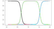
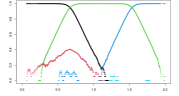
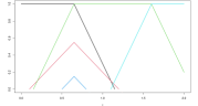
Figure 1. This figure depicts a simulation of a Moran model with mutation and selection (cf. Section 2.4) in the Gerish-Lenski regime with population size $N=500\,000$ and fitness increment distribution $\gamma=\frac{1}{2}\delta_{\{1\}}+\frac{1}{2}\delta_{\{2\}}$. Left: sub-population sizes divided by $N$, approximating logistic curves; middle: logarithmic sub-population sizes divided by $\log N$, approximately giving piecewise linear trajectories and making effects of clonal interference on the first (red) mutation visible; right: stylized version of these trajectories providing a good guess of the scaling limit – i.e. the PIT.

In order to become resident, i.e. the only clonal subpopulation whose logarithmic size is close to $\log N$ (cf. Remark 2.2), mutation $i$ has to overcome two hurdles: a) it must survive the “genetic drift”, i.e. the fluctuations caused by neutral reproduction, and b) it must then not be outcompeted by the offspring of a different clonal subpopulation. In phase a), it is decided whether mutation $i$ becomes contending or whether it is wiped out from the population. This typically lasts only a few generations. On the other hand, the competition addressed in b) lasts longer. Indeed, in the absence of other contending mutations, for $0<h<1$ it typically takes an order of $\log N/A_{i}$ generations until the size of the clonal subpopulation $i$ has increased to $N^{h}$.

During a period of length $\log N/A_{i}$, on average $(\mu_{N}\log N)/A_{i}$ new mutations will occur. This makes it plausible that, if $\mu_{N}$ is of smaller order than $1/\log N$, then there would be no clonal interference, and any contending mutation would go to fixation. On the other hand, if $\mu_{N}$ is of order at least $1/\log N$, and the distribution of the fitness increments does not scale with $N$, new mutations could arise and finally supersede the clonal population $i$, even if the latter may have grown already to an almost macroscopic subpopulation. This is the hallmark of clonal interference.

In this paper we consider the case when $\mu_{N}$ is of order $1/\log N$, which we refer to as the Gerrish–Lenski regime since it was proposed by the authors of [GL98]. Here we will focus on the case of strong selection, in which the distribution of the $A_{i}$ does not scale with $N$. As $N\to\infty$, the logarithms of the clonal subpopulation sizes divided by $\log N$ will, when considered on a timescale whose unit is $\log N$ generations, increase with initial slope $A_{i}$, given that mutation $i$ becomes a contender. On that timescale, and if $\mu_{N}=\lambda/\log N$ for some $\lambda>0$, new trajectories appear at the times of a Poisson process with intensity $\lambda$. The slopes of trajectories are reduced whenever the resident population changes, more precisely, at each resident change, the slope of each trajectory that is currently at a positive height is decreased by the amount by which the resident fitness has just increased. These kinks will hinder some clonal subpopulations from reaching residency, and may slow down the growth of even those subpopulations that eventually become resident.

Let us next describe the main results of the paper. In the framework of the Moran model defined in Section 2.4, Theorem 2.14 proves the convergence of the rescaled logarithmic frequencies of clonal subpopulations as $N\to\infty$ and with time sped up by $\log N$ (i.e., in the timescale of contending mutations), to the PIT. See Figure 1 for an illustration. As mentioned above we work here in a regime of strong selection. We leave the case of moderate selection (see [BGCPW21a] for a precise definition of moderate selection) for future work.

Our main result on the PIT concerns the existence of a speed of adaptation, i.e., the average increase of fitness. Denote by $F(t)$ the fitness of the resident at time $t>0$. We show in Theorem 2.8 that $F(t)/t$ converges almost surely as $t\to\infty$ to a deterministic limit (which is called the speed of adaptation). The limit is positive and finite whenever the distribution of fitness increments has a finite first moment, and infinite otherwise. In general, obtaining a precise numerical value or an easy-to-evaluate explicit formula for the speed seems difficult, and we postpone such investigations to future work.

In [GL98], the authors were particularly interested in a prediction of the slowing down of the speed of adaptation caused by clonal interference. Their heuristics consisted in eliminating contending mutations that are prevented to become resident by another, fitter mutation born after them. This heuristics was refined in [BGCPW19], using a “Poisson picture” which already carried certain features of the Poissonian interacting trajectories emerging from Theorem 2.14. In Section 3.5 we compare the heuristics from [GL98, BGCPW19] to a simulation study based on the PIT.

Next a few more words regarding previous work. The parameter regime of “rare mutations” (i.e. $\mu_{N}\ll\log N$) was considered e.g. in [GCKWY16]. In the setting of adaptive dynamics, the effects of clonal interference were analysed in [BS17, BS19]. The authors only studied the case of three competing types rigorously, and they mentioned in [BS19] that in order to obtain a scaling limit for recurrent mutations, the relevant mutation regime should be precisely the analogue of the Gerrish–Lenski regime. We also point out that piecewise linear trajectories describing the scaling limits of logarithmic frequencies of mutant families appear already in [DM11]. In fact, the authors consider polynomial (and thus much faster than inverse logarithmic) mutation rates per generation, leading to a regime where large numbers of “mutations on mutations” indeed occur already in the growth phase of a mutant family, such that random genetic drift plays asymptotically no role in the large-population limit. Another difference to our setting is that the authors of [DM11] consider deterministic fitness increments. These altogether lead to deterministic limiting systems. In Section 5.2 we discuss these prior results and other related ones in more detail, and we compare our setting and results to those in other regimes of the mutation rate.

The remainder of the paper is organized as follows. In Section 2 we present and discuss the models and main results in detail. Specifically, in Sections 2.1 and 2.2 we introduce the dynamics of interacting trajectories as well as the PIT, for which in Section 2.3 we state our first main result, Theorem 2.8, and further conclusions regarding the speed of adaptation. In Section 2.4 we specify the Moran model with recurrent beneficial mutations which via Theorem 2.14 presented in Section 2.5 justifies the PIT as a large-population scaling limit. The results of Section 2.3 will be proved in Section 3, while Section 4 concerns the proof of Theorem 2.14. Our findings are complemented in Section 5 by some further discussions and an outlook.

2. Model and main results

2.1. A system of interacting trajectories

We denote the space of continuous and piecewise linear trajectories from $[0,\infty)$ to $[0,1]$ by $\mathcal{C}_{\rm PL}$. Each $h\in\mathcal{C}_{\rm PL}$ has at time $t$ a height $h(t)$ and a (right) slope

$$v_{h}(t):=\lim\limits_{\delta\downarrow 0}\tfrac{1}{\delta}(h(t+\delta)-h(t)).$$ (2.1)

We define $\mathcal{C}_{\rm PL}^{\ast}:=\{h\in\mathcal{C}_{\rm PL}\mid(h(t),v_{h}(t))\in\mathcal{S}\mbox{ for all }t\geq 0\}$, where

$$\mathcal{S}:=\big{(}\{0\}\times[0,\infty)\big{)}\cup\big{(}(0,1)\times\mathbb{R}\big{)}\cup\big{(}\{1\}\times(-\infty,0]\big{)}.$$

Figure 2 displays a few trajectories in $\mathcal{C}_{\rm PL}^{\ast}$. Assume that for $k\in\mathbb{N}$ and $\overline{\iota}\in\mathbb{N}_{0}\cup\{\infty\}$ we are given two configurations

$$\aleph:=((\eta_{i},c_{i}))_{-k<i\leq 0}\in{\mathcal{S}}^{\{-k+1,\ldots,0\}}$$ (2.2)

with $(\eta_{i},c_{i})\neq(\eta_{i^{\prime}},c_{i^{\prime}})$ for $i\neq i^{\prime}$, $\eta_{i}<1$ for $i<0$,

$(\eta_{0},c_{0}):=(1,0)$, and

$$\beth:=((t_{i},c_{i}))_{1\leq i<\overline{\iota}}\in([0,\infty)^{2})^{\{i\,\mid 1\leq i<\overline{\iota}\}},$$ (2.3)

with $0<t_{1}<t_{2}\cdots$ and $t_{i}\uparrow\infty$ as $i\to\infty$ in case $\overline{\iota}=\infty$.

We view $\aleph$ as a starting configuration specifying the height and slope of trajectory $h_{i}$, $-k<i\leq 0$, at time $0$, and of $\beth$ as an immigration configuration, specifying that the trajectory $h_{i}$, $1\leq i<\overline{\iota}$, has height $0$ for $t\in[0,t_{i}]$ and right slope $c_{i}$ at its immigration time $t_{i}$. The symbols $\aleph$ (aleph) and $\beth$ (beth) are reminiscent of “being present at time 0” and “born later”.

Definition 2.1 (Interactive dynamics).

For a starting configuration $\aleph$ as in (2.2) and an immigration configuration $\beth$ as in (2.3), let

$$\mathbb{H}=\{h_{i}\mid-k<i<\overline{\iota}\}\in\big{(}\mathcal{C}_{\rm PL}^{\ast}\big{)}^{\aleph\,\cup\,\beth}$$ (2.4)

result from the following deterministic interactive dynamics on $\mathcal{S}^{\{i\in\mathbb{Z}|-k<i<\overline{\iota}\}}$:

• Trajectories continue with constant slope until the next immigration time is reached or one of the trajectories reaches either 1 from below or 0 from above.

• At the immigration time $t_{i}$ the slope of trajectory $h_{i}$ jumps from $0$ to $c_{i}$.

• Whenever at some time $t$ a trajectory reaches height $1$ from below, the slopes of all trajectories whose height is in $(0,1]$ at time $t$ are simultaneously reduced by

  $$v^{\ast}:=\max\limits\{v_{h}(t-)\mid h\in\mathbb{H}\mbox{ such that }h(t)=1\},$$

  i.e. for all $h\in\mathbb{H}$ with $h(t)>0$

  $$v_{h}(t):=v_{h}(t-)-v^{\ast}.$$ (2.5)

• Whenever a trajectory at some time $t$ reaches height $0$ from above, its slope is instantly set to $0$, and this trajectory then stays at height $0$ forever.

We call this $\mathbb{H}$ the system of interacting trajectories initiated by $\aleph$ and $\beth$, and denote it by $\mathbb{H}(\aleph,\beth)$.

Remark 2.2.

The intuition behind Definition 2.1 (which will be justified by the large-population limit of the Moran model defined in Section 2.4, see Theorem 2.14) is as follows:

Consider a population of size $N$ which at time $0$ consists of $k$ subfamilies, the one indexed with $i=0$ being of “macroscopic” size (i.e. logarithmically equivalent to $N$ as $N\to\infty$) and the others (indexed with $i=-1,...,-k+1$) being of “mesoscopic” size (i.e. logarithmically equivalent to $N^{h}$, $h\in(0,1)$). The initially resident type has fitness $f(0)$, while for $i<0$ type $i$ has fitness $c_{i}+f(0)$. Thus, as long as all the types with negative indices are mesoscopic, their sizes grow (in an appropriate timescale) exponentially with Malthusian $c_{i}$, which is equivalent to say that their “logarithmic sizes” (corresponding to $h_{i}$) grow linearly with slope $c_{i}$. At each time $t_{i}$ contained in the configuration $\beth$, a new type arises by a mutation on top of the currently resident type. The fitness increment of this new type is $c_{i}$, which is thus also its relative fitness with respect to the resident type at time $t_{i}$. Assume the first of all types apart from the initial resident that reaches a macroscopic size is type $j$, and assume this happens (under an appropriate time rescaling) at time $r>0$. Then at this time the resident fitness jumps from $f(0)$ to $f(0)+c_{j}$, and all the other types whose growth is still ongoing find themselves in an environment in which competition is more difficult: e.g. while the relative fitness (w.r.t. the resident) of type  $-1$ was $c_{-1}$ before time $r$, it jumps to $c_{-1}-c_{i}$ at time $r$, assuming its subpopulation has not been absorbed at $0$ yet, i.e. gone extinct. This allows us to specify the resident fitness $f(t)$ at time $t$ as in the next definition, and explains the “kinks” of the trajectories that happen at resident change times, illustrating the third bullet point in Definition 2.1. In this way, the notions “relative fitness of type $i$ with respect to the currently resident type” and “current slope of the trajectory $i$” become equivalent.

Definition 2.3 (Resident change times, resident type, and resident fitness).

Let $\mathbb{H}$ be as in (2.4), following the dynamics specified in Definition 2.1.

• The times at which one of the trajectories $h_{i}$, $i>-k$, reaches height $1$ from below will be called the resident change times.

• For $t>0$ we call

  $$\rho(t):=\arg\max\{v_{h_{i}}(t-)\colon-k<i<\overline{\iota},h_{i}(t)=1\},$$ (2.6)

  the resident type at time $t$.

• With $f(0)$ being chosen arbitrarily, we define the resident fitness $f(t)$, $t\geq 0$, by decreeing that $f$ at any resident change time $r$ has an upward jump with

  $$f(r)-f(r-)=\max\{v_{h}(r-)\mid h\in\mathbb{H},\,h(r)=1\}$$ (2.7)

and remains constant between any two subsequent resident change times.

Remark 2.4.

1. The resident fitness $f$ (as defined in (2.7)) obeys

   $$f(t)=c_{\rho(t)}+f(t_{\rho(t)}),\quad t\geq 0.$$ (2.8)

2. If $t\geq 0$ is not a resident change time, then $\rho(t)$ is the unique $i>-k$ for which $h_{i}(t)=1$. If $t$ is a resident change time and $h_{i}$ is the only trajectory that reaches height 1 from below at time $t$, then $\rho(t)=i$. More generally, $\rho(t)$ in (2.6) is the fittest of all types that are at height $1$ at time $t$.

3. In the special case of the starting configuration $\aleph=(1,0)$ (which will be most relevant in sequel), the resident type $\rho(t)$ defined in (2.6) satisfies (with $t_{0}:=0$)

   $$\rho(t)=\max\{i\mid 0\leq i<\overline{\iota},\,h_{i}(t)=1\}.$$ (2.9)

   Indeed, for two indices $i\neq i^{\prime}$ with $h_{i}(t)=h_{i^{\prime}}(t)=1$ one has $v_{h_{i}}(t-)<v_{h_{i}^{\prime}}(t-)$ if and only if $t_{i}<t_{i^{\prime}}$. This is true because using (2.5) it is easily checked that the difference between the (right) slopes of two trajectories is constant over all times as long as the height of both trajectories is positive.

Remark 2.5.

Putting $t_{i}:=0$ for $-k<i\leq 0$, and $\eta_{i}:=0$ for $i\geq 1$, the dynamics specified in Definition 2.1 for $t\geq 0$ translates into the following system of equations:

$$h_{i}(t) = \mathds{1}_{\{t\geq t_{i}\}}\Big{(}\eta_{i}+\int_{t_{i}}^{t}c_{i}+f(t_{i})-f(s)\mathrm{d}s\Big{)}^{+},\qquad-k<i<\overline{\iota},$$ (2.10)

$$f(t) = \max\{c_{j}+f(t_{j})\mid-k\leq j<\overline{\iota},\,h_{j}(t)=1\}.$$ (2.11)

Working in a piecewise manner (up to the next immigration or resident change time) one checks readily that for an arbitrary choice of $f(0)$ the system ((2.10), (2.11)) has a unique solution $(f,\mathbb{H})$, with $\mathbb{H}=(h_{i})_{-k\leq i<\overline{\iota}}$ following the dynamics specified in Definition 2.1, and $f$ being the resident fitness specified in Definition 2.3.

In the next subsection we will encounter a situation in which the population is initially monomorphic in the sense that $k=1$, i.e. $\aleph=((1,0))$.

2.2. Poissonian interacting trajectories

Consider the Poissonian sequence

$$\Psi:=((T_{i},A_{i}\cdot B_{i}))_{i\in\mathbb{N}},$$

where $((T_{i},A_{i}))_{i\in\mathbb{N}}$ (with $0<T_{1}<T_{2}<\cdots$) are the points of a Poisson process with intensity measure $\lambda\,{\rm d}t\,\gamma({\rm d}a)$, $(t,a)\in\mathbb{R}_{+}^{2}$, and, conditionally on $(T_{i},A_{i})_{i\geq 1}$, the random variables $B_{i}$ are independent and Bernoulli-distributed with

$$\mathbb{P}(B_{i}=1)=\frac{A_{i}}{1+A_{i}}.$$ (2.12)

We will refer to $\mathbb{H}(((1,0)),\Psi)=:(H_{i})_{i\in\mathbb{N}_{0}}=:\mathscr{H}$ as the system of Poissonian interacting trajectories with parameters $(\lambda,\gamma)$, or briefly as the ${\rm PIT}(\lambda,\gamma)$. The resident fitness in this system, which inherits its randomness from the Poissonian immigration configuration $\Psi$, will be denoted by $F=(F(t))_{t\geq 0}$.

Note that for $a>0$ the quantity $\frac{a}{1+a}$ is the survival probability of a binary, continuous-time Galton–Watson process with birth rate $1+a$ and death rate $1$, see e.g. [AN72, p. 109]. Likewise, $\frac{a}{1+a}$ is the fixation probability of a mutant with (strong) selective advantage $a$ in a standard Moran$(N)$-model as $N\to\infty$, see e.g. [BGCPW21b, Section 2.4].

Definition 2.6 (Genealogy of mutations in the PIT).

For $i\in\mathbb{N}$ we call $\rho(T_{i})$ (as defined in (2.6)) the parent of type $i$ in the PIT $\mathscr{H}$. In this case, we call type $i$ a child of $\rho(T_{i})$. This induces a random rooted tree $\mathscr{G}$ with vertex set $\mathbb{N}_{0}$, edge set $\{(\rho(T_{i}),i)\,|\,i\in\mathbb{N}\}$ and root $0$, which we call the ancestral tree of mutations in the PIT $\mathscr{H}$. Type $j$ is called an ancestor of type $i$ if there is a directed path from $j$ to $i$ in this tree. In that case, we also say that type $i$ is a descendant of type $j$.

The next remark explains the frequency of contending mutants and introduces some notation that will be useful for our discussions, further assertions and proofs.

Remark 2.7 (Discarding lines of initial slope $0$).

Let $\mathscr{H}$ be a PIT as just defined. The trajectories $H_{i}$ for which $B_{i}=0$ remain at height $0$ forever and thus will never be contending for residence. We observe newborn lines with initially positive slopes at times $T^{*}_{1}<T^{*}_{2}<\ldots$ where $\{T^{*}_{1},T^{*}_{2},\ldots\}:=\{T_{i}\mid B_{i}=1\}$. This thinning reduces the immigration rate $\lambda$ to

$$\lambda^{*}:=\lambda\int\frac{a}{1+a}\gamma({\rm d}a),$$ (2.13)

and the random variables $(A^{*}_{1},A^{*}_{2},\ldots)$ that come along with the $T^{*}_{j}$’s have a biased distribution, being i.i.d. copies of a random variable $A^{*}$ with

$$\mathbb{P}(A^{*}\in{\rm d}a)=\frac{\lambda}{\lambda^{*}}\cdot\frac{a}{1+a}\gamma({\rm d}a)=:\gamma^{*}({\rm d}a).$$

We call the trajectory born at time $T^{*}_{j}$ the $j$-th contending trajectory (or simply $j$-th contender). In view of Remark 2.2 we will address $T_{i}$ and $T^{*}_{j}$ also as the times of the $i$-th mutation and the $j$-th contending mutation, respectively.

Figure 2. This is an example of a realisation of a PIT with $(T_{1},\ldots,T_{6})=(0.1,0.3,0.9,1.2,1.6,2.5)$. The Bernoulli variables $B_{1}$, …, $B_{6}$ have realisations $0,1,1,0,1,1$ and the initial slopes of $H_{2},H_{3},H_{5},H_{6}$ are $(A_{2},A_{3},A_{5},A_{6})=(0.2,1,1.2,1.4)$. Among $H_{1},H_{2},\dots$, the trajectory $H_{3}$ is the first one to reach height $1$. At the time $R_{1}$ at which this happens, the slope of $H_{0}$ jumps from $0$ to $-1$, the slope of $H_{2}$ jumps from $0.2$ to $-0.8$ and the slope of $H_{5}$ jumps from $1.5$ to $0.5$. The numbers in the top line of the figure are the current values of the resident fitness $F(t)$. In particular, according to (2.11), $F(R_{2})=\max(A_{3}+F(T_{3}),A_{5}+F(T_{5}))=1.5$, and $F(R_{3})=\max(A_{5}+F(T_{5}),A_{6}+F(T_{6}))=2.4.$

2.3. Speed of adaptation in the PIT and related results

Again let $F(t)$ denote the resident fitness at time $t\geq 0$ in the PIT $\mathscr{H}$. In case the limit of $\frac{1}{t}F(t)$, as $t\to\infty$, exists in $[0,\infty]$, we call this the speed of increase of the resident fitness, or briefly the speed of adaptation. In the present section as well as in Section 3 we present rigorous results on the existence and value of this speed, and in Section 3.5 we discuss related heuristics. Our main result regarding the speed of adaptation is the following.

Theorem 2.8.

Let $\gamma\in\mathcal{M}_{1}((0,\infty))$.

1. If $\int_{0}^{\infty}a\gamma({\rm d}a)<\infty$, then, as $t\to\infty$, $\frac{1}{t}F(t)$ converges almost surely to a constant $\overline{v}\in(0,\infty)$.

2. If $\int_{0}^{\infty}a\gamma({\rm d}a)=\infty$, then $\frac{1}{t}F(t)\to\infty$ almost surely.

The proof of this theorem, which will be carried out in Section 3, is based on a renewal argument.

The next proposition is in the spirit of the thinning heuristics introduced in [BGCPW19, Section 3.1]; its proof will rely on Proposition 3.6 stated in Section  3.

Proposition 2.9.

In the case of deterministic and constant fitness advantages, i.e. if for some $c>0$ $\gamma=\delta_{c}$, we have a.s.

$$\lim_{t\to\infty}\frac{F(t)}{t}=\frac{\lambda c^{2}}{1+c+\lambda}=\frac{c^{2}\lambda^{*}}{c+\lambda^{*}}.$$ (2.14)

where (cf. (2.13)) $\lambda^{*}=\frac{\lambda c}{1+c}$ is the rate at which a new contender appears.

For $\lambda\to\infty$ the r.h.s. of (2.14) converges to $c^{2}$, reflecting the fact that high mutation rate leads to a strong effect of clonal interference. In a similar spirit is the next proposition, whose proof will also be given in Section  3. Roughly spoken it states that, in the presence of clonal interference with high mutation rates, many mutations are lost and the fitness increment over a fixed time interval is dictated by the mutations whose fitness increment is “essentially maximal”.

Proposition 2.10.

Let the support of $\gamma$ be bounded, with $b$ denoting its supremum. For $\lambda>0$ let $F_{\lambda}$ be the resident fitness in the PIT$(\lambda,\gamma)$. Then, for any $t>0$

$$F_{\lambda}(t)\xrightarrow{\lambda\to\infty}b(\lceil bt\rceil-1)\qquad\text{in probability.}$$

An estimate of the speed of adaptation can be obtained using the refined Gerrish–Lenski heuristics introduced in [BGCPW19], which is an improved variant of the Gerrish–Lenski heuristics [GL98]. We will review this briefly in Section 3.5. In Section 3.6 we lay the groundwork for these discussions via introducing the notion of fixation of mutants and making some first observations about it.

Extending the line of argument that led to Theorem 2.8, an application of the a functional central limit theorem for renewal reward processes (discussed in Appendix A) yields the following functional central limit theorem for the population fitness $F(t)$ in case of finite variance of $\gamma$. For convenience of notation, we assume $F(0)=m_{0}=0$; otherwise we consider $F(t)-m_{0}$ instead of $F(t)$.

Theorem 2.11.

If $\int_{0}^{\infty}a^{2}\gamma({\rm d}a)<\infty$, then there exists $\sigma>0$ such that

$$\Bigg{(}\frac{F(nt)-\overline{v}nt}{\sigma\sqrt{n}}\Bigg{)}_{t\geq 0}\overset{d}{\longrightarrow}W\quad\mbox{ as }n\to\infty,$$ (2.15)

where $\overline{v}$ is as in Theorem 2.8(i), $W=(W_{t})_{t\geq 0}$ is a standard Brownian motion and “$\overset{d}{\longrightarrow}$” denotes convergence in distribution in the space of càdlàg functions from $[0,\infty)$ to $\mathbb{R}$ with respect to the Skorokhod $J_{1}$-topology.

The standard deviation $\sigma$ figuring in (2.15) above will be expressed in (3.20) with the help of a renewal structure that will be defined in Section 3.

2.4. A Moran model with clonal interference

The prelimiting model which will figure in Theorem 2.14 is a Moran model with population size $N$ and infinitely many types. We now define its type space and its Markovian dynamics on the type frequencies. At time $0$ finitely many types (numbered by $-k+1,-k+2,\ldots,0$) are present, and after time $0$ new types (numbered by $1,2,\ldots$ in the order of their appearance) arrive in the population via mutations at the jump times of a Poisson counting process $\mathcal{I}^{N}(t)$, $t\geq 0$, with rate $\mu_{N}=\tfrac{\lambda}{\log N}$. For given numbers $f(0)$ and $c_{i}$, $-k<i<0$ and $c_{0}:=0$, the fitness levels of the types $-k+1,\cdots,-1,0$ that are present at time $t=0$ are defined as

$$m_{i}^{N}:=c_{i}+f(0),\qquad-k<i\leq 0{\color[rgb]{0,0,1}.}$$

For $t\geq 0$ and $i>-k$ we denote the number of type-$i$ individuals at time $t$ by $\mathcal{X}^{N}_{i}(t)$, and write $\mathcal{X}^{N}(t)=(\mathcal{X}^{N}_{i}(t))_{i>-k}$. We specify the joint Markovian dynamics of the process $(\mathcal{X}^{N},\mathcal{M}^{N},\mathcal{I}^{N})=(\mathcal{X}^{N}(t),\mathcal{M}^{N}(t),\mathcal{I}^{N}(t))_{t\geq 0}$, where $\mathcal{M}^{N}(t)=(M^{N}_{i})_{-k<i\leq\mathcal{I}^{N}(t)}$ is the vector of fitness levels of the types that came into play up to time $t$.

The state space of $(\mathcal{X}^{N},\mathcal{M}^{N},\mathcal{I}^{N})$ is

$$E_{N}:=\bigcup_{\iota\in\mathbb{N}_{0}}\Big{\{}(x_{-k+1},x_{-k+2}\ldots,x_{\iota},0,0,\ldots)\Big{|}x_{i}\in\mathbb{N}_{0},\sum_{-k<i\leq\iota}x_{i}=N\Big{\}}\times\mathbb{R}^{k+\iota}\times\{\iota\}.$$

Writing

$$e_{i}=(e_{i,\ell})_{\ell>-k}=(0,0,\ldots,0,1,0,0,\ldots)$$

for the sequence that has 1 in component $i$ and $0$ in all other components, we can write the transition rates as follows:

• Mutation: For $(x,m,\iota)\in E_{N}$, for $-k<j\leq\iota$ and $a\in\mathbb{R}_{+}$, the jump rate of the process $(\mathcal{X}^{N},\mathcal{M}^{N},\mathcal{I}^{N})$ from $(x,m,\iota)$ to $(x-e_{j}+e_{\iota+1},m+(m_{j}+a)e_{\iota+1},\iota+1)$ is $\frac{\lambda}{\log N}\frac{x_{j}}{N}\gamma({\rm d}a)$.
  

• Resampling: For $(x,m,\iota)\in E_{N}$ and for $-k<j,\ell\leq\iota$, the jump rate of the process $(\mathcal{X}^{N},\mathcal{M}^{N},\mathcal{I}^{N})$ from $(x,m,\iota)$ to $(x+e_{j}-e_{\ell},m,\iota)$ is $x_{j}x_{\ell}(1+(m_{j}-m_{\ell})^{+})\frac{1}{N}$.

In order to pass to a timescale in which one unit of time corresponds to $\log N$ generations, we define the process $(\mathscr{X}^{N},\mathscr{M}^{N},\mathscr{I}^{N})$ by

$$(\mathscr{X}^{N}(t),\mathscr{M}^{N}(t),\mathscr{I}^{N}(t)):=(\mathcal{X}^{N}(t\log N),\mathcal{M}^{N}(t\log N),\mathcal{I}^{N}(t\log N)).$$ (2.16)

The process $\mathscr{I}^{N}$ is thus for all $N$ a Poisson counting process with intensity $\lambda$. This allows to couple the sequence of processes $(\mathscr{X}^{N},\mathscr{M}^{N})$, $N\in\mathbb{N}$, via ingredients which we encountered already in Section 2.2:

• Let $(T_{i})_{i\in\mathbb{N}}$ be the times of a Poisson process of rate $\lambda>0$.

• Let $(A_{i})_{i\in\mathbb{N}}$ be an i.i.d. sequence of $\gamma$-distributed random variables that is independent of $(T_{i})_{i\in\mathbb{N}}$.

Remark 2.12.

a) Like $(\mathcal{X}^{N},\mathcal{M}^{N},\mathcal{I}^{N})$, the process $(\mathscr{X}^{N},\mathscr{M}^{N},\mathscr{I}^{N})$ defined by (2.16) is a Markovian jump process. Its dynamics may be specified using $(T_{i})$ and $(A_{i})$ as follows:

• Mutation: At time $T_{i}$ the process $(\mathscr{X}^{N},\mathscr{M}^{N},\mathscr{I}^{N})$ jumps from state $(x,m,\iota)$ to state $(x-e_{j}+e_{i},m+e_{i}\cdot(A_{i}+m_{j}),\iota+1)$ with probability $x_{j}/N$,  $-k<j$.
  (Note that, when a mutation event occurs as above, necessarily $i=\iota+1$.)
  

• Resampling: The process $(\mathscr{X}^{N},\mathscr{M}^{N},\mathscr{I}^{N})$ jumps from state $(x,m,\iota)$ to state $(x+e_{j}-e_{\ell},m,\iota)$ at rate $x_{j}x_{\ell}(1+(m_{j}-m_{\ell})^{+})\frac{\log N}{N}$,  $-k<j,\,\ell\leq\iota$.

b) The just described dynamics on the type frequencies can also be obtained via a graphical representation with three types of transitions:

1. a mutation occurs at each time $T_{i}$ on an individual that is randomly sampled from the population, resulting in the founder of a new type with fitness increment $A_{i}$ relative to its parent;

2. neutral reproduction occurs with rate proportional to $1/N$ for each ordered pair of individuals and leads to the first one reproducing (i.e., giving rise to another individual with the same type and fitness) and the second one dying;

3. selective reproduction occurs for each pair of individuals with rate proportional to $1/N$ times their fitness difference, and leads to the fitter individual reproducing and the less fit one dying.

Definition 2.13.

1. Using the just described graphical representation we can trace back the individual ancestral lineages and in particular define a genealogy of mutations: For $i>0$ we say that $j<i$ is the parent of type $i$ if type $i$ originated via a mutation of a type $j$-individual. In the case $k=1$ (i.e. if all individuals at time $0$ carry the same type) this induces a random tree $G^{N}$ with vertex set $\mathbb{N}_{0}$ and root $0$.

2. The logarithmic frequency (or briefly the height) of the $i$-th mutant family at time $t$ is defined as

   $$H^{N}_{i}(t) :=\frac{\log^{+}\big{(}\mathscr{X}^{N}_{i}(t)\big{)}}{\log N},\qquad\text{where }\log^{+}(x):=\log(1+x).\color[rgb]{0,0,0}$$ (2.17)

The sequence of random paths $H^{N}=(H^{N}_{i})$ takes values in $\mathcal{D}^{\mathbb{N}_{0}}$, where

$${\mathcal{D}}:={\mathcal{D}}(\mathbb{R}_{+},[0,1])$$ (2.18)

is the space of sequences of càdlàg functions from $\mathbb{R}_{+}$ to $[0,1]$, equipped with a metric that induces the Skorokhod $J_{1}$-convergence on all bounded time intervals, see [EK09] Sec. 3.5.

2.5. The PIT as a large-population scaling limit

For $N\in\mathbb{N}$ let $H^{N}$ be as in Section 2.4 with initial condition given by $k=1$ and $\mathscr{X}^{N}(0)=(N,0,0,\ldots)$. Let $M^{N}_{i}$ be the random fitness level of the $i$-th mutant. In terms of the representation given in Remark 2.12 we can (and will) define these quantities as

$$M^{N}_{i}:=\mathscr{M}^{N}_{i}(T_{i})$$ (2.19)

Let $\mathscr{H}$ be the system of Poissonian interacting trajectories with parameters $\lambda$ and $\gamma$ (defined in Section 2.2), and let $F(t)$ be the resident fitness in the PIT at time $t$. Put

$$M_{i}:=F(T_{i})+A_{i},$$ (2.20)

where $A_{i}$ is as in Section 2.2.7.

Theorem 2.14.

For all $i=1,2,\ldots$, as $N\to\infty$,

$$H^{N}\xrightarrow{\,\,d\,\,}\mathscr{H}\,\,\mbox{\rm as random elements of }\mathcal{D}^{\mathbb{N}_{0}},$$ (2.21)

$$(M_{1}^{N},\ldots,M_{i}^{N})\xrightarrow{\,\,d\,\,}(M_{1},\ldots,M_{i}),$$ (2.22)

$$G^{N}|_{\{0,\ldots,i\}}\xrightarrow{\,\,d\,\,}\mathscr{G}|_{\{0,\ldots,i\}},$$ (2.23)

where the random trees $G^{N}$ and $\mathscr{G}$ are specified in Definitions 2.13 and 2.6, respectively, and the set of trees with vertex set $\{0,1,\ldots,i\}$ that are rooted in $0$ is endowed with the discrete topology.

The following proposition indicates the importance of Theorem 2.8 by illustrating that the average population fitness in the Moran model – which essentially equals the fitness of the (mostly) unique macroscopic resident – approximates the resident fitness of the PIT.

Proposition 2.15.

Let $\overline{F}^{N}(t)=\frac{1}{N}\sum_{i=1}^{\mathscr{I}^{N}(t)}\mathscr{X}^{N}_{i}(t)\mathscr{M}^{N}_{i}(t)$ the average population fitness in the prelimiting Moran model. Then, as $N\to\infty$, $\overline{F}^{N}\xrightarrow{d}F$ with respect to the Skorokhod $M_{2}$-topology.

The proofs of Theorem 2.14 and Proposition 2.15 will be carried out in Section 4, starting with a short outline in Section 4.1. From the proof of Theorem 2.14 it is apparent that for any fixed $i$, the convergences (2.21)–(2.23) occur jointly in distribution (and not only separately for the three prelimiting objects).

3. The speed of adaptation and related results

3.1. Renewals in the Poissonian interacting trajectories.

We recall that $(H_{i})_{i=0,1,\ldots}$ is the PIT based on the sequence $(T_{i},A_{i}B_{i})_{i\in\mathbb{N}}$. For abbreviation we put, recalling (2.1),

$$V_{i}(t):=v_{H_{i}}(t)=\lim_{\delta\downarrow 0}\tfrac{1}{\delta}(H_{i}(t+\delta)-H_{i}(t)),$$ (3.1)

i.e. $V_{i}$ is the right derivative (slope) of the $i$-th trajectory. We can view $(H_{i}(t),V_{i}(t))_{i=0,1,\ldots}$ as the state at time $t$ of a Markovian system of particles whose dynamics (apart from the birth of particles given by the compound Poisson process $(T_{i},A_{i}B_{i})_{i\in\mathbb{N}}$) is deterministic and follows the interactive dynamics introduced in Definition 2.1. We recall from (2.6) that the resident (type) at time $t$ is

$$\rho(t)=\max\{i\in\mathbb{N}_{0}:H_{i}(t)=1\},$$

i.e. the a.s. unique $i\in\mathbb{N}_{0}$ for which $(H_{i}(t),V_{i}(t))=(1,0)$ (cf. Remark 2.4).

In accordance with Definition 2.3, the set of resident change times is

$$\mathscr{R}:=\{t>0\mid\rho(t-)\neq\rho(t)\}.$$

The fitness of types $i=1,2,\ldots$ is defined recursively as

$$M_{0}:=m_{0},\quad M_{i}:=M_{\rho(T_{i})}+A_{i},\quad i\geq 1.$$ (3.2)

Consequently, the population fitness $F(t)$ of the PIT at time $t$ (which was defined in Section 2.2)

$$F(t)=M_{\rho(t)}.$$ (3.3)

Noting that $B_{\rho(t)}=1$ whenever $\rho(t)>0$ and using the convention that $T_{0}=A_{0}=0$, combining (3.2) and (3.3) gives in accordance with (2.8),

$$F(t)=F(T_{\rho(t)})+A_{\rho(t)}.$$ (3.4)

The following remark is an immediate consequence of the definition of the PIT dynamics:

Remark 3.1.

For all $i\in\mathbb{N}$, as long as $H_{i}>0$, every jump of $V_{i}$ corresponds to a jump of $F$. More precisely, for all $t$ with $H_{i}(t)>0$,

$$V_{i}(t-)-V_{i}(t)=F(t)-F(t-).$$ (3.5)

Thus, for all $T_{i}\leq t<t^{\prime}$ with $H_{i}(t^{\prime})>0$, by summing over the residence change times between $t$ and $t^{\prime}$ we obtain

$$V_{i}(t)-V_{i}(t^{\prime})=F(t^{\prime})-F(t).$$ (3.6)

Lemma 3.2 (Decomposition of population fitness along resident change times).

$$F(t)=m_{0}+\sum_{r\in\mathscr{R}\cap[0,t]}V_{\rho(r)}(r-),\qquad t\geq 0.$$ (3.7)

Proof.

Recalling the definition of $\rho(t)$ and that $F(0)=m_{0}$, this follows directly by iterating (2.7). ∎

An immediate corollary of (3.7) is

$$F(t)-F(s)\leq\sum_{i:s<T_{i}\leq t}A_{i}B_{i},\qquad t>s\geq 0.$$ (3.8)

Definition 3.3 (Solitary resident changes).

We define the sequence of solitary resident change (SRC) times as those resident change times $L_{1}<L_{2}<\cdots$ for which $V_{i}(L_{n})\leq 0$   for all $i=1,2,\ldots$

Remark 3.4.

The just defined times $L_{n}$ initiate idle periods of the particle system, with the next resident still waiting for its birth. Since the trajectories $i$ for which $V_{i}(L_{n})<0$ never become resident after time $L_{n}$, we may forget about them and observe that $\mathbb{H}(((1,0)),\Psi)$ has the same distribution as $\mathbb{H}(((1,0)),\Psi_{n})$ , where (as in Section 2.2) $\Psi=((T_{i},A_{i}\cdot B_{i}))_{i\in\mathbb{N}}$, and

$$\Psi_{n}:=((T_{i_{n}+i-1}-L_{n},A_{i_{n}+i-1}\cdot B_{i_{n}+i-1}))_{i\in\mathbb{N}},$$

where $i_{n}:=\min\{j\in\mathbb{N}:T_{j}>L_{n}\}$. Thus the $L_{n}$ form regeneration (or renewal) times for the PIT. Intuitively, the restrictions of the PIT to the intervals $[L_{n},L_{n+1})$ can be seen as i.i.d. “clusters if trajectories”, whose concatenation renders the PIT. In particular,

$$F(L_{n})-F(0)=\sum_{\ell=1}^{n}(F(L_{\ell})-F(L_{\ell-1})),\quad n=1,2\ldots,$$ (3.9)

and the random variables $\big{(}L_{n}-L_{n-1},F(L_{n})-F(L_{n-1})\big{)}$, $n=1,2,\ldots$, are independent copies of $(L_{1},\Delta F)$, where

$$\Delta F:=F(L_{1})-F(0).$$ (3.10)

Lemma 3.5 (Cluster lengths have finite moments).

The first solitary resident change time $L_{1}$ obeys

$$\mathbb{E}[e{\alpha L_{1}}]<\infty\quad\text{ for some $\alpha>0$.}$$

In particular, $\mathbb{E}[L_{1}^{\nu}]<\infty$ for all $\nu\in\mathbb{N}.$

Proof.

1. Let $i\in\mathbb{N}$ be such that

$$A_{i}B_{i}>0\mbox{ and there is no }i^{\prime}\neq i\mbox{ with }B_{i^{\prime}}>0\mbox{ and }T_{i^{\prime}}\in\big{[}T_{i}-\tfrac{2}{A_{i}},T_{i}+\tfrac{2}{A_{i}}\big{]}.$$ (3.11)

We claim that as a consequence, the trajectory born at time $T_{i}$ becomes resident not later than $T_{i}+\frac{2}{A_{i}}$, and moreover that this resident change is solitary. To this purpose we first observe that any trajectory whose height $H_{k}(T_{i})$ is strictly positive must have been born at some time $T_{k}<T_{i}-\frac{2}{A_{i}}$ and hence must have at time $T_{i}$ a slope

$$V_{k}(T_{i})<\frac{A_{i}}{2}.$$ (3.12)

This is true because $t\mapsto V_{k}(t)$ is non-increasing on $[T_{k},\infty)$ (which is clear by Definition (2.1)) and becomes non-positive as soon as $H_{k}(t)$ has reached height 1. Let

$$R:=\sup\big{(}\{T_{i}\}\cup\{r\mid r\in\mathscr{R},\,\max_{t\leq r}H_{i}(t)<1\}\big{)}.$$

On the event $\{R=T_{i}\}$ there are no resident changes after $T_{i}$ until the trajectory born at time $T_{i}$ reaches height 1. Hence this trajectory keeps its initial slope $A_{i}$, reaches height 1 at time $T_{i}+\frac{1}{A_{i}}$ and at this time and kinks the slopes of all the trajectories whose height was positive at time $T_{i}$ to a negative value.

On the event $\{R>T_{i}\}$, put $k:=\rho(R)$. Observing that $V_{k}(R)=0$ we obtain from (3.6) (with $k$ in place of $i$) and (3.12)

$$F(R)-F(T_{i})=V_{k}(T_{i})-V_{k}(R)\leq\frac{A_{i}}{2}.$$

Likewise, observing that $V_{i}(T_{i})=A_{i}$, we obtain from (3.6)

$$V_{i}(R)-A_{i}=F(T_{i})-F(R)\geq-\frac{A_{i}}{2},$$

hence $V_{i}(R)\geq\frac{A_{i}}{2}$. Consequently, the trajectory born at time $T_{i}$ keeps a slope of at least $\frac{A_{i}}{2}$ until it becomes resident at some time $R^{\prime}\leq T_{i}+\frac{2}{A_{i}}$. Thus, all trajectories that were born before time $T_{i}-\frac{2}{A_{i}}$ and at time $R^{\prime}$ have height in $(0,1]$ are kinked to a negative slope at time $R^{\prime}$, and by assumption no contending trajectories except $H_{i}$ are born in the time interval $[T_{i}-\frac{2}{A_{i}},T_{i}+\frac{2}{A_{i}}]$. Hence $R^{\prime}$ is the time of a solitary resident change.

Figure 3. Illustration of part 1 of the proof of Lemma 3.5. Top: case $\{R>T_{i}\}$. Between times $T_{i}-2/A_{i}$ and $T_{i}+2/A_{i}$ there is no birth time apart from $T_{i}$, while we have $V_{i}(T_{i})=A_{i}B_{i}=2$. All slopes of trajectories that are still positive at time $T_{i}$ are at most $A_{i}/2$, and hence the $i$-th trajectory reaches height 1 at time $R^{\prime}\leq T_{i}+2/A_{i}$ at latest, kinking all other trajectories with current heights in $(0,1]$ to a negative slope. In the picture, the only trajectory still having a positive slope at time $T_{i}$ is the brown one, and $R$ is the time when this trajectory reaches height 1. The slope of the brown trajectory in $[T_{i},R)$ equals $0.5$, and thus at time $R$, the blue trajectory is kinked to slope $2-0.5=1.5\geq A_{i}/2$. The gray trajectory corresponds to the mutant who is resident at time $T_{i}$ (this is the last resident before the brown one).
Bottom: case $\{R=T_{i}\}$. Now the brown mutant is absent, so that the blue trajectory suffers no kink before reaching height 1, and the previous resident before the blue one is the gray one. Note that here, the time when the blue trajectory reaches height 1 is $R=T_{i}+1/A_{i}$.

2. Let $i_{0}:=\min\{i\in\mathbb{N}\mid i\mbox{ has property }\eqref{solitarycond}\}$. We claim that $i_{0}<\infty$ a.s. and that $\mathbb{E}[e^{\alpha R_{0}}]<\infty$ for some $\alpha>0$, where $R_{0}$ is the time at which the trajectory born in $T_{i_{0}}$ becomes resident. To see this, consider the Poisson point process $\Phi:=\sum_{i\in\mathbb{N}}\delta_{(T_{i},A_{i}B_{i})}$. Let $a_{0}>0$ be such that $\gamma([a_{0},\infty))>0$. For $n\in\mathbb{N}$ we define the sets $C_{n}$, $D_{n}\subset\mathbb{R}_{+}\times\mathbb{R}_{+}$ and the events $E_{n}$ by

$$C_{n}:=\big{[}\tfrac{5n+2}{a_{0}},\tfrac{5n+3}{a_{0}}\big{]}\times[a_{0},\infty),\quad D_{n}:=\Big{(}\Big{[}\tfrac{5n}{a_{0}},\tfrac{5n+5}{a_{0}}\Big{]}\times\mathbb{R}_{+}\Big{)}\setminus C_{n},$$

$$E_{n}:=\{\Phi(C_{n})=1\}\cap\{\Phi(D_{n})=0\}.$$

The events $E_{n}$ are independent and have a probability that does not depend on $n$. Due to our choice of $a_{0}$ this probability is positive. Therefore, the random variable $K:=\min\{n\mid{\mathchoice{1\mskip-4.0mu\mathrm{l}}{1\mskip-4.0mu\mathrm{l}}{1\mskip-4.5mu\mathrm{l}}{1\mskip-5.0mu\mathrm{l}}}_{E_{n}}=1\}$ is a geometric random variable with a positive parameter. This implies that $\mathbb{E}[e{\alpha^{\prime}K}]<\infty$ for some $\alpha^{\prime}>0$. Since by construction $R_{0}\leq\frac{5(K+1)}{a_{0}}$, it is enough to take $\alpha=a_{0}\alpha^{\prime}/5$.

3. Because of step 1, the resident change time $R_{0}$ found in step 2 is solitary. Obviously, $L_{1}\leq R_{0}$, and thus $\mathbb{E}[e{\alpha L_{1}}]<\infty$ with $\alpha>0$ as in step 2. ∎

3.2. Proof of Theorem 2.8

Theorem 2.8 is a direct consequence of the following proposition, which in turn relies on the just proved key Lemma 3.5.

Proposition 3.6.

a)   Almost surely, $\lim\limits_{t\to\infty}\tfrac{F(t)-F(0)}{t}$   exists, and equals $\overline{v}:=\frac{\mathbb{E}[\Delta F]}{\mathbb{E}[L_{1}]}$.

b)   $\overline{v}\leq\lambda\mathbb{E}[A_{1}B_{1}]$.

c) $\overline{v}<\infty$ if and only if $\int_{0}^{\infty}a\,\gamma(da)<\infty$.

Proof.

In view of Remark 3.4,

$$\widehat{F}(t):=\sum_{i\geq 1}{\mathchoice{1\mskip-4.0mu\mathrm{l}}{1\mskip-4.0mu\mathrm{l}}{1\mskip-4.5mu\mathrm{l}}{1\mskip-5.0mu\mathrm{l}}}_{\{L_{i}\leq t\}}(F(L_{i})-F(L_{i-1}))=\sum_{i=0}^{\infty}F(L_{i})\mathds{1}_{[L_{i},L_{i+1})}(t),\qquad t\geq 0,$$ (3.13)

is a renewal reward process, and thanks to Lemma 3.5 assertion a) is a quick consequence of the law of large numbers. For convenience of the reader we recall the argument. For $t\geq 0$ let $n(t)$ be such that $L_{n(t)}\leq t<L_{n(t)+1}$. Then

$$\frac{(F(L_{n(t)})-F(0))/n(t)}{L_{n(t)+1}/n(t)}\leq\frac{F(t)-F(0)}{t}\leq\frac{(F(L_{n(t)+1})-F(0))/n(t)}{L_{n(t)}/n(t)}$$ (3.14)

Since

$\bullet\quad n(t)\to\infty$ a.s. as $t\to\infty$,

$\bullet\quad L_{n}$ is a sum of i.i.d. copies of $L_{1}$ which has finite expectation by Lemma 3.5,

$\bullet\quad F(L_{n})$ is a sum of i.i.d. copies of $\Delta F$ defined in (3.10),

both the left and the right hand side of (3.14) converge a.s. to $\frac{\mathbb{E}[\Delta F]}{\mathbb{E}[L_{1}]}$. This proves assertion a).

To show assertion b) we first observe that the strong law of large numbers for renewal processes gives the a.s. convergence $\frac{1}{t}\sum_{i:T_{i}<t}A_{i}B_{i}\to\lambda\mathbb{E}[A_{1}B_{1}]\mbox{ as }t\to\infty.$ Combining this with (3.8) results in assertion b).

We now turn to the proof of c). From the definition of $\overline{v}$ and Lemma 3.5 it follows that $\overline{v}<\infty$ if and only if $\mathbb{E}[\Delta F]<\infty$. On the other hand, the finiteness of $\int a\gamma(da)$ clearly is equivalent to the finiteness of $\mathbb{E}[A_{1}B_{1}]=\int a\frac{a}{a+1}\gamma(da)$. In view of the proposition’s part b) it thus only remains to show that $\mathbb{E}[\Delta F]$ is infinite provided $\gamma$ has infinite expectation. This, however, follows from the estimate

$$\mathbb{E}[\Delta F]\geq\mathbb{E}[A_{1}{\mathchoice{1\mskip-4.0mu\mathrm{l}}{1\mskip-4.0mu\mathrm{l}}{1\mskip-4.5mu\mathrm{l}}{1\mskip-5.0mu\mathrm{l}}}_{\{A_{1}B_{1}\geq 1\}\cap\{T_{1}<1\}\cap\{T_{2}\geq 2\}}].\hfill\qed$$

3.3. Proof of Propositions 2.9 and 2.10

Proof of Proposition 2.9..

Let $T$ be the time at which the first contending mutation appears. The time $T$ has an exponential distribution whose parameter is $\lambda^{*}=\lambda\frac{c}{1+c}$, the intensity of the birth process of contending mutations. The first contending mutation becomes resident at time $R:=T+\frac{1}{c}$, and all contending mutations that are born in the time interval $(T,R)$ are kinked to slope $0$ at time $R$. This means that $R$ is the first solitary resident change time $L_{1}$ specified in Definition 3.3. This time has expectation

$$\mathbb{E}[L_{1}]=\mathbb{E}[T]+\frac{1}{c}=\frac{1}{\lambda^{*}}+\frac{1}{c}=\frac{c+\lambda^{*}}{c\lambda^{*}},$$

and the “renewal reward” $\Delta F=F(L_{1})-F(0)$ has the deterministic value $c$. Thus, the assertion of Proposition 2.9 follows directly from Proposition 3.6 a). ∎

Proof of Proposition 2.10..

Consider the system $\mathbb{H}(\aleph,\beth)$ where $\aleph=((1,0),(0,b))$ and $\beth=((\frac{i}{b},b))_{i\geq 1}$. There, at time $0$ immediately a line starts with slope $b$ and, just as that hits $1$, the next line starts with slope $b$ and so on. In this system, the resident fitness will always jump up by $b$ at times $i/b$, $i\in\mathbb{N}$, and thus equals $b\lfloor bt\rfloor$ at any time $t$. This system describes a best case scenario for the PIT$(\lambda,\gamma)$ in this proposition, in the sense that the resident fitness of the PIT$(\lambda,\gamma)$ obeys $F_{\lambda}(t)\leq b\lfloor bt\rfloor$. Since $\mathbb{P}(F_{\lambda}(\frac{1}{b})=b)=0$, we obtain for all $t$ that almost surely $F_{\lambda}(t)$ is bounded from above by the left-continuous version of $t\mapsto b\lfloor bt\rfloor$, i.e. $F_{\lambda}(t)\leq b(\lceil bt\rceil-1)$.

For a lower bound let $\Psi_{\lambda}$ be a Poisson point process of intensity $\lambda dt\otimes\gamma$, fix $\varepsilon\in(0,\frac{b}{2})$ and note that the probability of the event

$$E_{\lambda}:=\{\Psi_{\lambda}\cap[0,\varepsilon)\times[b-\varepsilon,b]=\varnothing\},\qquad\text{i.e.\ }e^{-\lambda\varepsilon\gamma([b-\varepsilon,b])},$$

tends to $0$ as $\lambda\to\infty$. Now, note that outside of $E_{\lambda}$ there is at least one mutant line born before time $\varepsilon$ of slope at least $b-\varepsilon$. Hence, the first change of resident will be at the latest at time $\varepsilon+\frac{1}{b-\varepsilon}$ and will add fitness of at least $(\varepsilon+\frac{1}{b-\varepsilon})^{-1}$. At that moment, all other contenders will be kinked to a slope of at most $\varepsilon<b-\varepsilon$. From there, we can iterate and obtain

$$F(t)\geq\Big{(}\varepsilon+\frac{1}{b-\varepsilon}\Big{)}^{-1}\Bigg{(}\Big{\lceil}\Big{(}\varepsilon+\frac{1}{b-\varepsilon}\Big{)}^{-1}t\Big{\rceil}-1\Bigg{)}$$

on an event of probability $\mathbb{P}(E_{\lambda}^{c})^{\lfloor(\varepsilon+\frac{1}{b-\varepsilon})^{-1}t\rfloor}\to 1$. Since $(\varepsilon+\frac{1}{b-\varepsilon})^{-1}\nearrow b$, as $\varepsilon\to 0$, the proposition holds. ∎

3.4. Proof of Theorem 2.11

1. In order to apply the result of Appendix A to the renewal reward process $\widehat{F}$ defined in (3.13), we have to check that, under our assumption that $\int_{0}^{\infty}a^{2}\gamma({\rm d}a)<\infty$,

$$\mathbb{E}[F(L_{1})^{2}]<\infty.$$ (3.15)

In order to exploit the independence properties of the Poisson process $(T_{i},A_{i}B_{i})_{i\geq 1}$ we work with the random variable $K$ defined in the proof of Lemma 3.5 and set out to show that

$$\mathbb{E}\Big{[}F\Big{(}\tfrac{5(K+1)}{a_{0}}\Big{)}^{2}\Big{]}<\infty.$$ (3.16)

In view of $L_{1}\leq 5(K+1)/a_{0}$ and the estimate (3.7) we have

$$F(L_{1})\leq F\Big{(}\tfrac{5(K+1)}{a_{0}}\Big{)}\leq\sum_{n=0}^{K}{X_{n}}$$ (3.17)

where

$$X_{n}:=\sum_{i\geq 1}{\mathchoice{1\mskip-4.0mu\mathrm{l}}{1\mskip-4.0mu\mathrm{l}}{1\mskip-4.5mu\mathrm{l}}{1\mskip-5.0mu\mathrm{l}}}_{\big{\{}\tfrac{5n}{a_{0}}\leq T_{i}<\tfrac{5(n+1)}{a_{0}}\big{\}}}A_{i}B_{i},\quad n\geq 0.$$

Thus for proving (3.15) it suffices to show that the second moment of the r.h.s. of (3.17) is finite. By definition of $K$ and from the second moment assumption on $\gamma$,

$$\mathbb{E}[X_{K}^{2}]=\mathbb{E}[A_{1}^{2}\mid A_{1}B_{1}\geq a_{0}]=\int_{a_{0}}^{\infty}a^{2}\tfrac{a}{a+1}\gamma({\rm d}a)\bigg{/}\int_{a_{0}}^{\infty}\tfrac{a}{a+1}\gamma({\rm d}a)<\infty.$$

We know from the proof of Lemma 3.5 that $\mathbb{E}[K^{2}]<\infty$. Hence the finiteness of the second moment of the r.h.s. of (3.17) is guarenteed if we can show that

$$\mathbb{E}[X_{n}^{2}\mid n<K]=c<\infty$$ (3.18)

with $c$ not depending on $n$. For this we use the terminology from the proof of Lemma 3.5. Both $\Phi(C_{n})$ and $\Phi(D_{n})$ are Poisson random variables with parameters $\alpha_{C}$ and $\alpha_{D}$ that depend only on $\lambda,\gamma$ and $a_{0}$. Letting $E_{n}^{c}=\{\Phi(C_{n})\neq 1\}\cup\{\Phi(D_{n})\neq 0\}$, note that $\mathbb{E}[X_{n}^{2}\mid n<K]=\mathbb{E}[X_{n}^{2}\mid\cap_{k=1}^{n}E_{k}^{c}]=\mathbb{E}[X_{n}^{2}\mid E_{n}^{c}]$ since $X_{n}$ is independent of ${\mathchoice{1\mskip-4.0mu\mathrm{l}}{1\mskip-4.0mu\mathrm{l}}{1\mskip-4.5mu\mathrm{l}}{1\mskip-5.0mu\mathrm{l}}}_{E_{k}}$ for $k\neq n$. We write $X_{n}=X_{C,n}+X_{D,n}$, with

$$X_{C,n}:=\sum_{i:(T_{i},A_{i})\in C_{n}}A_{i}B_{i},\qquad X_{D,n}:=\sum_{i:(T_{i},A_{i})\in D_{n}}A_{i}B_{i}$$

The random variables $X_{C,n}$ and $X_{D,n}$ are measurable w.r.t. the random point measures $\Phi\big{|}_{C_{n}}$ and $\Phi\big{|}_{D_{n}}$, respectively. Conditioning these random point measures under the event $E_{n}^{c}$ affects only the number of their points in the sets $C_{n}$ and $D_{n}$ and not the distribution of the points’ locations. Recalling that $\gamma^{*}(da)=\tfrac{a}{1+a}\gamma(da)\big{/}\int\tfrac{a^{\prime}}{1+a^{\prime}}\gamma(da^{\prime})$, let $Y_{C}$ and $Y_{D}$ be random variables with distribution $\gamma^{*}\big{|}_{[a_{0},\infty)}\big{/}\gamma^{*}([a_{0},\infty)$ and $\gamma^{*}$, respectively. The above considerations imply

$$\mathbb{E}[X_{n}^{2}\,|\,E_{n}^{c}] \leq 2\big{(}\mathbb{E}[X_{C,n}^{2}\,|\,E_{n}^{c}]+\mathbb{E}[X_{D,n}^{2}\,|\,E_{n}^{c}]\big{)}$$ (3.19)

$$\leq 2\big{(}\mathbb{E}[\Phi(C_{n})^{2}\,|\,E_{n}^{c}]\,\mathbb{E}[Y_{C}^{2}]+\mathbb{E}[\Phi(D_{n})^{2}\,|\,E_{n}^{c}]\,\mathbb{E}[Y_{D}^{2}]\big{)}.$$

Our second moment assumption on $\gamma$ implies that both $\mathbb{E}[Y_{C}^{2}]$ and $\mathbb{E}[Y_{D}^{2}]$ are finite.

A Poisson random variable $Z$ with arbitrary parameter $\alpha$ fulfils

$$\mathbb{E}[Z^{2}|Z\neq 1]=\tfrac{\alpha(\alpha+1-e^{-\alpha})}{1-\alpha e^{-\alpha}}=:f_{1}(\alpha),\qquad\mathbb{E}[Z|Z>0]=\tfrac{\alpha(\alpha+1)}{1-e^{-\alpha}}=:f_{2}(\alpha).$$

Consequently,

$$\mathbb{E}[\Phi(C_{n})^{2}\mid E_{n}^{c}]\leq\max(\alpha_{C}(\alpha_{C}+1),f_{1}(\alpha_{C}))=:\beta_{C},\quad\mathbb{E}[\Phi(D_{n})\mid E_{n}^{c}]\leq f_{2}(\alpha_{D})=:\beta_{D}.$$

This shows that the r.h.s. of (3.19) is finite, and completes the proof of (3.15).

2. The quantity

$$\sigma^{2}:=\frac{\mathbb{E}[(F(L_{1})-\overline{v}L_{1})^{2}]}{\mathbb{E}[L_{1}]}$$ (3.20)

is finite by (3.15) and Lemma 3.5, and positive since the random variable $F(L_{1})-\overline{v}L_{1}$ is not almost-surely constant. Then Theorem A.1 applied to the renewal reward process $\widehat{F}$ implies

$$\Bigg{(}\frac{\widehat{F}(nt)-\overline{v}nt}{\sigma\sqrt{n}}\Bigg{)}_{t\geq 0}\overset{d}{\longrightarrow}W\quad\mbox{as}\quad n\to\infty.$$ (3.21)

It is plain that $\widehat{F}(t)\leq F(t)$ for all $t\geq 0$. On the other hand, considering

$$\widetilde{F}(t)=\sum_{i=0}^{\infty}F(L_{i+1})\mathds{1}_{[L_{i},L_{i+1})}(t),$$

we have $\widetilde{F}(t)\geq F(t)$ for all $t$. In order to conclude, it suffices to show that, for any $M>0$,

$$\sup_{t\in[0,M]}\frac{\widetilde{F}(nt)-\widehat{F}(nt)}{\sqrt{n}}\overset{n\to\infty}{\longrightarrow}0\qquad\text{in probability},$$

since this will imply that the Skorokhod distance between diffusive rescalings of $\widehat{F}$ and $F$ will go to zero in probability and hence (3.21) will be valid with $F$ in place of $\widehat{F}$ as well. To that end, denote by $N_{t}=\sup\{n\in\mathbb{N}\colon\,L_{n}\leq t\}$ (with $\sup\varnothing=0$) the number of SRC times up to time $t$, and note that $\widehat{F}(t)=F(L_{N_{t}})$, $\widetilde{F}(t)=F(L_{N_{t}+1})$. By [EKM97, Theorem 2.5.10],

$$\lim_{t\to\infty}\frac{N_{t}}{t}=\frac{1}{\mathbb{E}[L_{1}]}\quad\text{almost surely,}$$ (3.22)

and $\mathbb{E}[L_{1}]\in(0,\infty)$ by Lemma 3.5. Now, for $M,\varepsilon>0$,

$$\mathbb{P}\Big{(}\sup_{t\in[0,M]}\widetilde{F}(nt)-\widehat{F}(nt)>\varepsilon\sqrt{n}\Big{)}$$

$$\leq \mathbb{P}(N_{nM}>2nM/E[L_{1}])+\mathbb{P}\big{(}\exists k\leq 2nM/E[L_{1}]\colon\,F(L_{k+1})-F(L_{k})>\varepsilon\sqrt{n}\big{)}$$

$$\leq \mathbb{P}(N_{nM}>2nM/E[L_{1}])+(2nM/E[L_{1}]+1)\mathbb{P}(F(L_{1})>\varepsilon\sqrt{n}).$$

The first term in the r.h.s. above goes to zero as $n\to\infty$ by (3.22), and the second term also goes to zero because $F(L_{1})$ is square-integrable. This concludes the proof. ∎

3.5. Heuristics for the speed of adaptation

Gerrish and Lenski [GL98] proposed a heuristic for predicting the speed of adaptation which can be formulated and discussed in our framework as follows.

Consider a contender born at time $T^{*}_{i}$ with fitness increment $A^{*}_{i}$, and let $E_{i}$ be the event that its trajectory is not kinked by a previous resident change. On the event $E_{i}$, this contender becomes solitary resident if and only if between times $T^{*}_{i}$ and $T_{i}^{*}+(A_{i}^{*})^{-1}$ there is no birth of another contender whose fitness increment is larger than $A^{*}_{i}$. In other words, given the event $E_{i}$ and given $A_{i}^{*}=a$, the contender becomes solitary resident with probability

$$\pi_{\text{GL}}(a) =\exp\Big{(}-\frac{\lambda^{*}}{a}\gamma^{*}((a,\infty))\Big{)},\quad a>0.$$

Retaining only such mutations (and neglecting the relevance of the events $E_{i}$) leads to the following prediction of the speed:

$$\overline{v}_{\text{GL}}:=\lambda^{*}\int a\,\pi_{\text{GL}}(a)\,\gamma^{*}({\rm d}a).$$ (3.23)

Ignoring negative effects from the past by assuming $E_{i}$ naturally constitutes an overestimation of the speed, as confirmed in Figure 4.

The refined Gerrish–Lenski heuristics (rGLh) introduced in [BGCPW19] takes into account not only the future but also the past, by the following consideration:
Denote by $K_{i}=\{j<i\mid T^{\ast}_{j}<T^{\ast}_{i}<T^{\ast}_{j}+(A^{\ast}_{j})^{-1},A^{\ast}_{j}\geq A^{\ast}_{i}\}$. This is the set of mutations $j$ born prior to $i$ that would kink the $i$th trajectory to a negative slope before it reaches $1$ and hence prohibit its residency; provided that no further interference occurs. The rGLh now suggests the event $\{|K_{i}|=0\}$ as an approximation of $E_{i}$ leading to an (estimated) retainment probability given $A^{\ast}_{i}=a$ of

$$\pi_{\text{rGL}}(a) =\pi_{\text{GL}}(a)\cdot\exp\Big{(}-\lambda^{*}\int_{[a,\infty)}\frac{1}{b}\gamma^{*}({\rm d}b)\Big{)},$$

and the prediction $\overline{v}_{\text{rGL}}$ for the speed is as in (3.23), now with $\pi_{\text{rGL}}$ in place of $\pi_{\text{GL}}$.

While Figure 4 confirms that this gives a generally much more accurate estimate than the GLh, in most cases it underestimates the speed of adaptation. Indeed there exist instances of configurations where out of three consecutive mutations, the first and the last one contribute to the eventual increase of the population fitness and the middle one does not, in spite of the fact that only the middle one would be retained according to the refined Gerrish–Lenski heuristics, see Figure 5 for an example. This may (at least partially) explain this underestimation. We defer the analysis of this phenomenon, as well as possible further improvements of the heuristics, to future work.

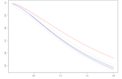
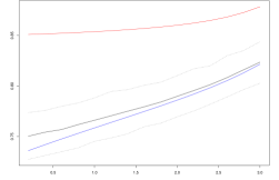
$\lambda^{*}$                                                                                                              $\sigma$

Figure 4. Simulations of speed of adaptation via $R_{1000}/\sum_{i:T_{i}^{*}\leq 1000}A_{i}^{*}$ with $1000$ iterations. Black line: mean, black dotted: $95\%$ confidence interval, red: GLh, blue: rGLh. Left: For each parameter $\lambda^{*}\in\{0.1,0.2,\ldots,1.9,2\}$ simulation with $\gamma^{*}=\text{Exp}(1/\lambda^{*})$. As $\lambda^{*}$ increases, expected sum of total increments remains constant, while effects of clonal interference increase (more mutations, longer fixation times) and hence the speed declines. Right: $\lambda^{*}=1$ and for each $\sigma\in\{0.2,0.4,\ldots,2.8,3\}$ we choose $\gamma^{*}=\text{unif}([3-\sigma,3+\sigma])$. With $\sigma$, the variance of $\gamma^{*}$ (i.e. $\sigma^{2}/3$) increases while its mean remains constant.

Figure 5. A realisation of the PIT in which the second of three consecutive contending mutations (path shown by red solid line) does not contribute to the eventual increase in population fitness, while the first and the third one does contribute (paths shown by blue and green solid lines). In contrast to this, the refined Gerrish–Lenski heuristics (see Sec. 3.5) would not take into account the first kink of the red trajectory and would rather see the first trajectory as being killed by the second one. This would lead to the continuation of the second trajectory by the dashed red line, and thus also to a killing of the third trajectory according to the rGLh.

3.6. Ancestral relations and fixations

In our prelimiting Moran model, a mutation is said to have gone to fixation as soon as all individuals in the population are descendants of the mutant individual (i.e. the founder of the corresponding clonal type). Analogously (recalling Definition 2.6) a mutation $i$ in a PIT is said to fix (or to reach fixation) by time $t$ if it is an ancestor of all mutations $j\neq i$ such that $H_{j}(t)>0$. Clearly, only contending mutations have a chance to fix (recall the notion of contenders from Remark 2.7). Considering the initial condition of the PIT, we see that the initial resident (which we count as type 0) fixes by time 0. It is also clear that if a mutation fixes at a certain time, then all its ancestors have gone to fixation by that time.

Remark 3.7.

(Fixation and solitary resident changes)

1. In a PIT $\mathscr{H}$, the $i$-th mutation fixes provided it becomes resident and its resident change time is solitary. Indeed, assume that mutation $i$ becomes resident at some time $r$. If there is no trajectory $H$ in $\mathscr{H}$ with $v_{H}(r)>0$, then no mutation that happened before $r$ will become resident after time $r$, and all the mutations happening after time $r$ will be descentants of $i$. A consequence of this assertion is that in the case when fitness advantages are deterministic and fixed, ever becoming resident implies eventual fixation. This is true because in this case, every resident change is solitary (cf. the proof of Proposition 2.9 in Section 3.2.)

2. Conversely, it may happen that a mutation (born at a time $t>0$) goes to fixation even though the time $r$ at which it reaches residency is not solitary. This is the case if a trajectory born between times $t$ and $r$ and keeping a positive slope $v(r)$ is surpassed by a trajectory that is born after time $r$, but afterwards a descendant (not necessarily a child) of the first trajectory manages to reach residency via a solitary resident change.

3. As a consequence of a) and b), the event whether the mutation born at time $T_{i}$ goes to fixation is not measurable w.r.t. the past of $T_{i}$, but it is measurable w.r.t. the past of the first solitary resident change time after $T_{i}$.

4. It may well happen that the clonal subpopulation founded by a mutant goes extinct before the corresponding mutation fixes. For an example, see Figure 2. Here, mutation 6 becomes resident at a solitary resident change time. Hence mutation 6 as well as its parent, mutation 3, go to fixation. However, before this happens, the type 3 subpopulation goes extinct due to its interference with the type 5 subpopulation, which in turn is outcompeted by type 6.

5. In summary, let us consider three attributes of contending mutations:
   AAA(R) UAS becoming resident,
   AAA(UA) SR becoming ultimately ancestral, i.e. going to fixation,
   AAA(SR) UA becoming solitary resident.
   For these we have the implications

   $$\mbox{(SR)}\Rightarrow\mbox{(UA)}\Rightarrow\mbox{(R)}.$$

6. In terms of the genealogy of mutations in the PIT introduced in Definition 2.6, we see that mutation $i$ fixes if and only if the subtree of the ancestral tree $\mathscr{G}$ rooted at $i$ is infinite. Recall that every (UA)-mutation is ancestral to all mutations born after this mutation became resident. Further, recall from Lemma 3.5 that the expected number of mutations between two subsequent (SR)-mutations is finite. In this sense, (SR)-mutations constitute bottlenecks in the genealogy while (UA)-mutations form the unique infinite path of $\mathscr{G}$.

4. The PIT as a scaling limit

4.1. Outline of the proof

As the very basis for the proof, in Section 4.2 we state results on super- and subcritical binary branching processes (Lemmas 4.1 and  4.2 resp.), regarding convergence to piecewise linear functions under logarithmic scaling. In Section 4.3, these findings will first be transferred to the Moran model without mutations in the presence of finitely many mutant families of mesoscopic size, to show linear growth of these mesoscopes between resident changes, cf. Lemma 4.4, using stochastic ordering via comparison of jump rates. Similarly, using time-change and stochastic ordering for bundles of mesoscopes, Lemma 4.5 handles said resident changes, showing that their time span indeed vanishes on the logarithmic time scale, providing a kink in the PIT. These evolutionary phases will then be pieced together by concatenating applications of Lemmas 4.4 and 4.5 along resident change times. In Sections 4.4 and 4.5, the proof of Theorem 2.14 will be completed by an induction along the times of mutations. Here, an essential intermediate step is Proposition 4.10, in which the logarithmic type frequencies of the $N$-th prelimiting system are coupled with a system of interacting trajectories as defined in Section 2.2, but now with the Bernoulli random variables $B_{i}$ replaced by indicators $B^{N}_{i}$ which predict whether the $i$-th mutant becomes a contender in the prelimit.

Possible generalizations of this methodology will be discussed in Section 4.8.

4.2. Auxiliary results from branching processes

The two lemmata in this subsection reflect the well-known fact that the logarithm of sped-up sub- or supercritical Galton–Watson (GW) processes scale to linear functions. In order to state them, let $Z=(Z_{t})_{t\geq 0}$ be a continuous-time binary Galton–Watson process with individual birth and death rates $b,d\geq 0$ respectively, and let $s:=|b-d|$. We denote by $T_{0}:=\inf\{t\geq 0\mid Z_{t}=0\}$ the extinction time, and by $\mathbb{P}_{z}$ the law of $Z$ started at $z\in\mathbb{N}_{0}$.

The next lemma follows from Theorem C.1, which gathers some useful facts in the supercritical case.

Lemma 4.1.

Assume $b>d$, abbreviate $\{Z\not\to 0\}:=\{Z_{t}\geq 1,\forall t\geq 0\}$ and let $z_{N}\in\mathbb{N}$, $N>1$. Then

1. $\displaystyle\sup_{t\geq 0}\Big{|}\frac{\log^{+}(Z_{t\log N})}{\log N}-\Big{(}\frac{\log z_{N}}{\log N}+st\Big{)}{\mathchoice{1\mskip-4.0mu\mathrm{l}}{1\mskip-4.0mu\mathrm{l}}{1\mskip-4.5mu\mathrm{l}}{1\mskip-5.0mu\mathrm{l}}}_{\{Z\not\to 0\}}\Big{|}\xrightarrow{N\to\infty}0$ in probability under $\mathbb{P}_{z_{N}}$;

2. If $t_{N}\to\infty$ then $\mathbb{P}_{z_{N}}(T_{0}\geq t_{N})\sim\mathbb{P}_{z_{N}}(Z\not\to 0)=1-(d/b)^{z_{N}}$ as $N\to\infty$.

The proof of the next lemma can be obtained as in [CMT21, Lemma A.1].

Lemma 4.2.

Assume $b<d$ and let $z_{N}\in\mathbb{N}$, $N>1$ with $\frac{\log z_{N}}{\log N}\to h\in[0,\infty)$ as $N\to\infty$. Then

1. $\displaystyle\sup_{0\leq t\leq t_{0}}\Big{|}\frac{\log^{+}(Z_{t\log N})}{\log N}-(h-st)^{+}\Big{|}\xrightarrow{N\to\infty}0$ in probability under $\mathbb{P}_{z_{N}}$ for any $t_{0}>0$;

2. $\frac{T_{0}}{\log N}\xrightarrow{N\to\infty}\frac{h}{s}$ in probability under $\mathbb{P}_{z_{N}}$.

Another useful property of binary Galton-Watson processes is the following: For $z<g\in\mathbb{N}$,

$$\begin{array}[]{ll}\mathbb{P}_{z}(Z\text{ reaches }g\text{ before it reaches }0)\leq\frac{z}{g}&\text{ when }b\leq d,\\ \mathbb{P}_{g}(Z\text{ reaches }z\text{ in finite time})=(d/b)^{g-z}&\text{ when }b>d.\end{array}$$ (4.1)

Indeed, the discrete-time embedding of $Z$ is a simple random walk on $\mathbb{N}_{0}$ with probability $p=b/(d+b)$ to jump to the right, so (4.1) follows from the well-known gambler’s ruin formula. For the first item, note that the subcritical case can be compared to the critical one. See also eq. (27) in [Cha06].

4.3. Selective sweeps in the presence of multiple mesoscopic types

Throughout this section we fix a $k\in\mathbb{N}$ (the number of types in the Moran model) and an $m\in\mathbb{R}_{+}^{k}$ (the vector of fitnesses). For $N\in\mathbb{N}$ let $X^{N}(t)=(X^{N}_{1}(t),\ldots,X^{N}_{k}(t))$, $t\geq 0$, be a process on

$${\mathcal{S}}_{N}^{k}:=\Big{\{}x=(x_{1},\ldots,x_{k}):x_{\ell}\in\mathbb{N}_{0},\sum_{\ell=1}^{k}x_{\ell}=N\Big{\}}$$

whose generator $L$ acts on functions $f:{\mathcal{S}}_{N}^{k}\to\mathbb{R}$ as

$$Lf(x)=\tfrac{\log N}{N}\sum_{i\neq j}x_{i}x_{j}(1+(m_{j}-m_{i})^{+})(f(x+e_{j}-e_{i})-f(x)).$$ (4.2)

This is the generator of a Moran model with selection accelerated by a factor $\log N$. In accordance with (2.17) we put for all $t\geq 0$ and $\ell=1,\ldots,k$

$$H^{N}_{\ell}(t):=\frac{\log^{+}\big{(}X^{N}_{\ell}(t)\big{)}}{\log N}.$$ (4.3)

For starting values $x^{N}_{\ell}$ of $X^{N}$ (with $x^{N}_{\ell}\in\{0,1,\ldots,N\}$) and corresponding starting heights $\eta^{N}_{\ell}:=\log^{+}(x^{N}_{\ell})/\log N$, $\ell=1,\ldots,k$, we assume that the asymptotic initial height

$$\eta_{\ell}:=\lim_{N\to\infty}\eta^{N}_{\ell}\mbox{ exists.}$$ (4.4)

We begin with some rough linear bounds on $H^{N}$.

Lemma 4.3.

Assume (4.4) and set $m_{\star}:=\max_{1\leq\ell\leq k}m_{\ell}$. For any $T,\varepsilon>0$,

$$\lim_{N\to\infty}\mathbb{P}\Big{(}\exists t\in[0,T]\colon\max_{1\leq\ell\leq k}\big{|}H^{N}_{\ell}(t)-\eta_{\ell}\big{|}\geq(1+m_{\star})t+\varepsilon\Big{)}=0.$$ (4.5)

Proof.

By the union bound, it is enough to consider a fixed $1\leq\ell\leq k$. Let us compare $X^{N}_{\ell}$ with two continuous-time Galton-Watson processes $Y$ and $Z$ with individual birth/death rates $0$/$\log N(1+m_{\star})$ and $\log N(1+m_{\star})$/$0$ respectively, both started from $X^{N}_{\ell}(0)$. Setting $\varphi:\mathcal{S}^{k}_{N}\to\mathbb{N}_{0}$, $\varphi(x)=x_{\ell}$, $E_{0}=\mathcal{S}^{k}_{N}$ and using (4.2), it is straightforward to verify condition (B.1) with $A$ the generator of $X$ and $B$ the generator of $Y$ or $Z$, implying that $X^{N}_{\ell}$ can be coupled with $Y$ and $Z$ so that $Y(t)\leq X^{N}_{\ell}(t)\leq Z(t)$ for all $t\geq 0$; note that Theorem B.1 only couples two processes, but the three processes can be coupled using regular conditional probabilities and taking $Y,Z$ e.g. conditionally independent given $X^{N}_{\ell}$. The claim (4.5) then follows from Lemmas 4.1–4.2 once we note that $Y,Z$ are sped-up versions (with time sped-up by $\log N$) of processes treated therein. ∎

Via comparison of jump rates as in Lemma 4.3, we will show in the next lemma that, in a multitype Moran process with a single macroscopic component, all the other components are close enough to independent branching processes so that their logarithmic frequencies on the $\log N$ timescale converge to linear functions, as long as none of these components become close to macroscopic.

Lemma 4.4 (Until the first resident change).

Fix a sequence $(\overline{h}_{N})$ in $(0,1)$ with the properties

$$\lim_{N\to\infty}\overline{h}_{N}=1\quad\mbox{ and }\quad(1-\overline{h}_{N})\log N\to\infty\,\mbox{ as }N\to\infty.$$ (4.6)

Suppose that  (i) $x_{1}^{N}\sim N$ as $N\to\infty$ (and consequently $\eta_{1}=1$),
Suppose that  (ii) $N^{\eta_{\ell}^{N}}=o\big{(}N^{\overline{h}_{N}}\big{)}$ as $N\to\infty$ for $\ell\geq 2$, and
Suppose that  (iii) If $m_{\ell}>m_{1}$ then $\eta_{\ell}<1$ and $\exists$ $\lim_{N\to\infty}x^{N}_{\ell}\in\mathbb{N}\cup\{\infty\}$.
Define

$$\overline{T}^{N}:=\inf\{t\geq 0\mid\max_{\ell\geq 2}H_{\ell}^{N}(t)\geq\overline{h}_{N}\}\in(0,\infty],$$ (4.7)

$$\tau:=\min\big{\{}\tfrac{1-\eta_{\ell}}{m_{\ell}-m_{1}}\mid\ell=2,\ldots,k;\,m_{\ell}>m_{1}\big{\}}\in(0,\infty]$$ (4.8)

where $\inf\varnothing=\min\varnothing=\infty$. Then for each $\ell\in\{1,\ldots,k\}$ the following holds.

1. If either $m_{\ell}\leq m_{1}$ or $x_{\ell}^{N}\to\infty$, the sequence of processes $(H_{\ell}^{N}(t))_{0\leq t\leq\overline{T}^{N}}$ converges to the map

   $$h_{\ell}:t\mapsto(\eta_{\ell}+(m_{\ell}-m_{1})t)^{+}$$

   in probability locally uniformly in $t\in[0,\overline{T}^{N}]$ in the sense that, for each $t_{0},\varepsilon>0$,

   $$\mathbb{P}\Big{(}\sup_{t\leq\overline{T}^{N}\wedge t_{0}}\Big{|}H_{\ell}^{N}(t)-h_{\ell}(t)\Big{|}>\varepsilon\Big{)}\xrightarrow{N\to\infty}0.$$

   Moreover, $\sup_{0\leq t<\overline{T}^{N}}\big{|}H_{1}^{N}(t)-1\big{|}\to 0$ in probability as $N\to\infty$.

2. On the other hand, assume that $m_{\ell}>m_{1}$ and that $\lim_{N\to\infty}x^{N}_{\ell}=x^{\infty}_{\ell}\in\mathbb{N}$. Let $\pi_{\ell}:=1-(1+m_{\ell}-m_{1})^{-x^{\infty}_{\ell}}<1$ and define $t^{N}:=\tfrac{1}{\sqrt{\log N}}$. Then the random variables

   $$B^{N}_{\ell}:={\mathchoice{1\mskip-4.0mu\mathrm{l}}{1\mskip-4.0mu\mathrm{l}}{1\mskip-4.5mu\mathrm{l}}{1\mskip-5.0mu\mathrm{l}}}_{\{X_{\ell}^{N}(t^{N})\geq\log N\}}\quad\text{satisfy}\quad\mathbb{P}(B^{N}_{\ell}=1)\sim\mathbb{P}(X_{\ell}^{N}(t^{N})\geq 1)\sim\pi_{\ell}\text{ as }N\to\infty.$$ (4.9)

   Moreover, for each $t_{0}>0$,

   $$\sup_{0\leq t\leq\overline{T}^{N}\wedge t_{0}}\big{|}H_{\ell}^{N}(t)-B^{N}_{\ell}[\eta_{\ell}+(m_{\ell}-m_{1})t]\big{|}\xrightarrow{N\to\infty}0\text{ in probability.}$$ (4.10)

3. Let $\tau^{N}:=\inf\{\tfrac{1-\eta_{\ell}}{m_{\ell}-m_{1}}\mid m_{\ell}>m_{1},B_{\ell}^{N}=1\}$, where $\inf\varnothing:=\infty$. Then

   $$\big{|}\overline{T}^{N}-\tau^{N}\big{|}\,\mathds{1}_{\{\tau^{N}<\infty\}}+\big{|}\mathds{1}_{\{\tau^{N}=\infty\}}-\mathds{1}_{\{\overline{T}^{N}=\infty\}}\big{|}\xrightarrow{N\to\infty}0\quad\mbox{in probability}.$$

   In particular, if $\eta_{\ell}>0$ for all $\ell=1,\ldots,k$, then $\overline{T}^{N}\to\tau$ in probability.

Proof.

We first observe that, for $x\in\mathcal{S}^{k}_{N}$ and $\ell\in\{2,\ldots,k\}$,

$$\frac{\log^{+}(x_{\ell})}{\log N}\leq\overline{h}_{N}\Longleftrightarrow 1+x_{\ell}\leq N^{\overline{h}_{N}}=:{\overline{g}}_{N}.$$ (4.11)

Moreover, because of (4.6)

$$\tfrac{\overline{g}_{N}}{N}\to 0\quad\mbox{as }N\to\infty.$$ (4.12)

Consequently, for $t\leq\overline{T}^{N}$,

$$\tfrac{\log(X^{N}_{1}(t))}{\log N}\geq\tfrac{\log(N-k\overline{g}_{N})}{\log N}=\tfrac{\log(1-k\overline{g}_{N}/N)+\log N}{\log N}\to 1\quad\mbox{ as }N\to\infty,$$

verifying the claim for $\ell=1$ in (1).

For $\ell\geq 2$, the generator (4.2) tells that, when $X^{N}$ is in state $x$, the total rate for its $\ell$-coordinate to increase by one is $x_{\ell}\cdot\beta_{\ell,N}(x)\log N$ and the total rate to decrease is $x_{\ell}\cdot\delta_{\ell,N}(x)\log N$, where

$$\beta_{\ell,N}(x) :=\frac{1}{N}\sum_{i\neq\ell}x_{i}\big{(}1+(m_{\ell}-m_{i})^{+}\big{)}\quad\text{and}\quad\delta_{\ell,N}(x):=\frac{1}{N}\sum_{i\neq\ell}x_{i}\big{(}1+(m_{i}-m_{\ell})^{+}\big{)}.$$

We are now going to sandwich $\beta_{\ell,N}(x)$ and $\delta_{\ell,N}(x)$ between the individual birth and death rates of two Galton-Watson processes. For this purpose we note (with a view on (4.12)) that for all $x\in\mathcal{S}_{N}^{k}$ which satisfy (the r.h.s. of) (4.11) one has, for $K>0$ and $N\in\mathbb{N}$ large enough, the estimates

$$\beta_{\ell,N}(x)\geq\tfrac{1}{N}(N-k\overline{g}_{N})(1+(m_{\ell}-m_{1})^{+})\geq(1-\tfrac{1}{K})(1+(m_{\ell}-m_{1})^{+})=:\beta^{-}_{\ell,K},$$

$$\beta_{\ell,N}(x)\leq 1+(m_{\ell}-m_{1})^{+}+\tfrac{1}{N}k\overline{g}_{N}(1+\max_{i\geq 2}(m_{\ell}-m_{i})^{+}))$$

$$\phantom{AAAAAA}\leq 1+(m_{\ell}-m_{1})^{+}+\tfrac{1}{K}(1+\max_{i\geq 2}(m_{\ell}-m_{i})^{+}))=:\beta^{+}_{\ell,K},$$

and similarly,

$$\delta_{\ell,N}(x)\geq\tfrac{1}{N}(N-k\overline{g}_{N})(1+(m_{1}-m_{\ell})^{+})\geq 1-\tfrac{1}{K}=:\delta^{-}_{\ell,K},$$

$$\delta_{\ell,N}(x)\leq 1+(m_{1}-m_{\ell})^{+}+\tfrac{1}{K}(1+\max_{i\geq 2}(m_{i}-m_{\ell})^{+}))=:\delta^{+}_{\ell,K}.$$

Let $Y^{K}_{\ell}$, $Z^{K}_{\ell}$ be continuous-time Galton-Watson processes with individual birth/death rates $\beta^{-}_{\ell,K}$/$\delta^{+}_{\ell,K}$ and $\beta^{+}_{\ell,K}$/ $\delta^{-}_{\ell,K}$ respectively. Setting $\varphi:\mathcal{S}^{k}_{N}\to\mathbb{N}_{0}$, $\varphi(x)=x_{\ell}$ and $E_{0}=\{x\in\mathcal{S}^{k}_{N}\colon\,x_{i}<\overline{g}_{N}~{}\forall i\geq 2\}$, we can reason as in Lemma 4.3 to couple $X^{N}_{\ell}$, $Y^{K}_{\ell}$ and $Z^{K}_{\ell}$ such that $Y^{K}_{\ell}(0)=X^{N}_{\ell}(0)=Z^{K}_{\ell}(0)$ and

$$Y^{K}_{\ell}(t\log N)\leq X^{N}_{\ell}(t)\leq Z^{K}_{\ell}(t\log N)\;\;\forall\,0\leq t\leq\overline{T}_{N}.$$ (4.13)

Moreover, by restarting $Y^{K}$, $Z^{K}$ at time $\overline{T}_{N}\log N$ and coupling them afterwards via Theorem B.1, we can make sure that also $Y^{K}(t)\leq Z^{K}(t)$ for all $t\geq 0$.

Note that $\beta^{\pm}_{\ell,K}\to 1+(m_{\ell}-m_{1})^{+}$ and $\delta^{\pm}_{\ell,K}\to 1+(m_{1}-m_{\ell})^{+}$, i.e., the birth and death rates of $Y^{K}_{\ell}$ and $Z^{K}_{\ell}$ become arbitrarily close, as $K\to\infty$, to $1+(m_{\ell}-m_{1})^{+}$ and $1+(m_{1}-m_{\ell})^{+}$ respectively.

Define next

$$\overline{T}^{N}_{\ell}:=\inf\big{\{}t\geq 0\mid H^{N}_{\ell}(t)\geq\overline{h}_{N}\big{\}},\;\ell\geq 2\quad\text{ and }\quad\widehat{T}^{N}:=\min\{\overline{T}^{N}_{\ell}\mid\ell\geq 2,m_{\ell}>m_{1}\}.$$ (4.14)

Let us show that w.h.p. (with high probability, i.e. with probability tending to $1$),

$$\overline{T}^{N}=\widehat{T}^{N}\quad\text{ and }\quad\overline{T}^{N}>t_{*}$$ (4.15)

for some constant $t_{*}>0$. Indeed, if $m_{\ell}\leq m_{1}$ and $K$ is large enough so that $Z^{K}_{\ell}$ is subcritical, then by (4.13), (4.1) and assumption (ii),

$$\mathbb{P}(\overline{T}^{N}_{\ell}=\overline{T}^{N})\leq\mathbb{P}_{x^{N}_{\ell}}(Z^{K}_{\ell}\text{ reaches }\overline{g}_{N}\text{ before }0)\leq\frac{x^{N}_{\ell}}{\overline{g}_{N}}\to 0.$$ (4.16)

This proves the equality in (4.15), and the inequality follows for $\widehat{T}^{N}$ in place of $\overline{T}^{N}$ by assumption (iii) and Lemma 4.3. In particular this implies that $\overline{T}^{N}=\infty$ w.h.p.  if $m_{\ell}\leq m_{1}$ for all $\ell$.

Consider now case (2), i.e. $m_{\ell}>m_{1}$ and $\pi_{\ell}<1$. Choosing $K$ large enough such that $Y^{K}_{\ell}$ is supercritical, let us show that, as $N\to\infty$,

$$\mathbb{P}_{x^{N}_{\ell}}\big{(}Y^{K}_{\ell}(\sqrt{\log N})\geq\log N\big{)}\sim\mathbb{P}_{x^{N}_{\ell}}\big{(}Y^{K}_{\ell}(\sqrt{\log N})\geq 1\big{)}\sim 1-\Bigg{(}\frac{\delta_{\ell,K}^{+}}{\beta_{\ell,K}^{-}}\Bigg{)}^{x^{\infty}_{\ell}}.$$ (4.17)

Indeed, the second equivalence follows by Lemma 4.1b). For the first, note that the first probability above is not larger than the second and not smaller than

$$\mathbb{P}_{x^{N}_{\ell}}\Big{(}Y^{K}_{\ell}\text{ reaches }2\log N\text{ by time }\sqrt{\log N},Y^{K}_{\ell}(\sqrt{\log N})\geq\log N\Big{)}$$

$$\geq \mathbb{P}_{x^{N}_{\ell}}\Big{(}Y^{K}_{\ell}\text{ reaches }2\log N\text{ by time }\sqrt{\log N}\Big{)}-\big{(}\delta^{+}_{\ell,K}/\beta^{-}_{\ell,K}\big{)}^{\log N}$$

by (4.1). Thus parts 3b) and 3c) of Theorem C.1 finish the proof of (4.17).

Using the same arguments for $Z^{K}_{\ell}$ as well as (4.13) and the inequality in (4.15), it follows that

$$1-\Bigg{(}\frac{\delta_{\ell,K}^{+}}{\beta_{\ell,K}^{-}}\Bigg{)}^{x^{\infty}_{\ell}} \leq\liminf_{N\to\infty}\mathbb{P}(B^{N}_{\ell}=1)\leq\limsup_{N\to\infty}\mathbb{P}(B^{N}_{\ell}=1)$$

$$\leq\liminf_{N\to\infty}\mathbb{P}(X^{N}_{\ell}(t^{N})\geq 1)\leq\limsup_{N\to\infty}\mathbb{P}(X^{N}_{\ell}(t^{N})\geq 1)\leq 1-\Bigg{(}\frac{\delta_{\ell,K}^{-}}{\beta_{\ell,K}^{+}}\Bigg{)}^{x^{\infty}_{\ell}},$$

and since both left- and right-hand sides above converge to $\pi_{\ell}$ as $K\to\infty$, we verify (4.9).

Now note that, since $\{Y^{K}_{\ell}\text{ survives}\}\subset\{Z^{K}_{\ell}\text{ survives}\}$ and both events have asymptotically equal probability as $K\to\infty$, with probability tending to $1$ either both survive or both die out. By (4.13) and (4.17) (and its analogue for $Z^{K}_{\ell}$), w.h.p., in the first case $B^{N}_{\ell}=1$ and in the second case $B^{N}_{\ell}=0$. In each case, by Lemma 4.1, $\frac{\log^{+}(Y^{K}_{\ell}(t\log N))}{\log N}$ and $\frac{\log^{+}(Z^{K}_{\ell}(t\log N))}{\log N}$ approximate, as $N\to\infty$ (in probability uniformly in $t\geq 0$) two lines which, for $K\to\infty$, converge to either $\eta_{\ell}+(m_{\ell}-m_{1})t$ or to $0$, respectively. Together with (4.13) again, this shows (4.10) and completes the proof of (2).

The proof of (1) works analogously in the supercritical case by noting that $\pi_{\ell}=1$ when $x^{N}_{\ell}\to\infty$, while the subcritical case is proved via application of Lemma 4.2 instead of Lemma 4.1. For the critical case acknowledge that $Y^{K}_{\ell}$ is subcritical and $Z^{K}_{\ell}$ supercritical, converging to two lines under the above scaling as $N\to\infty$, which both approach a constant line as $K\to\infty$.

Finally, by (4.15) it is enough to show (3) for $\widehat{T}^{N}$ under the assumption that $m_{\ell}>m_{1}$ for some $\ell\geq 2$. If $B^{N}_{\ell}=0$ for all such $\ell$, (4.10) and assumption (iii) imply that $\overline{T}^{N}=\infty$ w.h.p. If $B^{N}_{\ell}=1$ for some $\ell\geq 2$ with $m_{\ell}>m_{1}$, then $\tau^{N}$ is bounded; thus the assumption that $|\overline{T}^{N}-\tau^{N}|>\varepsilon$ for some $\varepsilon>0$ leads to a contradiction with (4.10) where either $X^{N}_{\ell}(\overline{T}^{N})<\overline{g}_{N}$ for all $\ell\geq 2$ or $X^{N}_{\ell}(t)>N$ for some $t>0$ and $\ell\geq 2$. This completes the proof of (3). ∎

As a complement to Lemma 4.4, the next lemma considers the case where one macroscopic component gets invaded by a fitter component starting from ‘almost’ macroscopic size, while all other components are mesoscopic. We will show that the time it takes until the first component becomes mesoscopic and the second component becomes macroscopic is asymptotically negligible on the $\log N$-timescale and leaves the remaining $\log$-scaled mesoscopic type sizes asymptotically unchanged. Together with Lemma 4.4 this reflects the well-known fact that the time required for a single advantageous mutation to go from a small fraction of a population to a big fraction close to one is negligible compared to the time which the mutant’s offspring needs to reach a small fraction of the population.

Again, let $X^{N}$ be a $\mathcal{S}^{k}_{N}$-valued process with generator (4.2) and initial conditions $x^{N}_{\ell}\in\mathbb{N}_{0}$, $1\leq\ell\leq k$, and assume that the asymptotic initial heights $\eta_{\ell}$ as in (4.4) are well defined.

Lemma 4.5 (Change of resident).

Suppose that, for some $\ell_{\star}\in\{2,\ldots,k\}$,

1. $x^{N}_{1}\sim N$ (and consequently $x^{N}_{\ell}=o(N)$ for $\ell=2,\ldots,k$) as $N\to\infty$,

2. $\eta_{\ell_{\star}}=1$ and $m_{\ell_{\star}}>m_{1}$,

3. $\max\big{\{}m_{\ell}:\ell\notin\{1,\ell_{\star}\}\text{ and }\eta_{\ell}=1\big{\}}<m_{\ell_{\star}}$ (where $\max\varnothing=-\infty$).

Let $\varepsilon_{N}>0$ satisfy $\varepsilon_{N}\to 0$ and $\varepsilon_{N}\log N\to\infty$ as $N\to\infty$. Define

$$\mathscr{T}^{N}:=\inf\big{\{}t\geq 0\mid X^{N}_{\ell_{\star}}(t)\geq N(1-\varepsilon_{N})\big{\}}.\vspace{-0.5em}$$ (4.18)

Then the following holds:

1. $\mathscr{T}^{N}\to 0$ in probability;

2. $\sup_{t\in[0,\mathscr{T}^{N}]}|H^{N}_{\ell}(t)-\eta_{\ell}|\to 0$ in probability for all $\ell\in\{1,\ldots,k\}$.

Proof.

Without loss of generality we may assume that $\ell_{\star}=2$. Let us first show (1) in the case $k=2$, in which $X^{N}_{2}$ is Markovian. Let $Y$ be a continuous-time Galton-Watson process started from $Y(0)=x^{N}_{2}$ with individual birth and death rates $(1+m_{2}-m_{1})$ and $1$ respectively, and set $s:=m_{2}-m_{1}$. Let $\delta_{N}>0$ satisfy $\delta_{N}\to 0$ and $\log(1/\delta_{N})/(\varepsilon_{N}\log N)\to 0$ as $N\to\infty$ (e.g. $\delta_{N}=e^{-\sqrt{\varepsilon_{N}\log N}}$). Define $\tau^{N}_{0}:=\inf\{t\geq 0\colon\,Y(t\log N)\geq\delta_{N}N\}$, and $\tau^{N}:=\inf\{t\geq 0\colon\,Y(t\log N)\geq N(1-\varepsilon_{N})\}$. Since $\tau_{0}^{N}\leq\tau^{N}\leq\inf\{t\geq 0\colon\,Y(t\log N)\geq N\}$, Theorem C.1 3c) implies that, with high probability, $\tau_{0}^{N}\leq\tfrac{2}{s}[1-\log(x^{N}_{2})/\log N]$. Moreover, since $\tau^{N}-\tau_{0}^{N}$ under $\mathbb{P}_{x^{N}_{2}}(\cdot\mid\tau_{0}^{N}<\infty)$ has the same distribution as $\tau^{N}$ under $\mathbb{P}_{\lceil\delta_{N}N\rceil}$, $\tau^{N}-\tau^{N}_{0}\leq\frac{2}{s}\log(1/\delta_{N})/\log N$.

Define $\phi:\{0,\ldots,N\}\to(0,\infty)$ by $\phi(x)=1-(x\wedge\lceil N(1-\varepsilon_{N})\rceil)/N$ and introduce the time-change

$$S_{t}:=\int_{0}^{t}\frac{1}{\phi(Y_{u})}du.$$

Note that $\phi(x)\geq\varepsilon_{N}-N^{-1}\geq\tfrac{1}{2}\varepsilon_{N}$ for large $N$ so that $S_{t}$ is continuous, strictly increasing and $\lim_{t\to\infty}S_{t}=\infty$. The relation between the generators of $X^{N}_{2}$ and $Y$ shows that $X^{N}_{2}(t\wedge\mathscr{T}^{N})_{t\geq 0}$ has the same distribution as $(Z_{\sigma_{t}\wedge\tau^{N}})_{t\geq 0}$ where $\sigma_{t}$ is the inverse of $S_{t}$ (see e.g. [EK09, Section 6.1]). In particular, $\mathscr{T}^{N}$ is equal in distribution to $S_{\tau^{N}}$. Since, for large $N$, $\phi(x)\geq 1/2$ for $x\leq\varepsilon_{N}N$,

$$S_{\tau^{N}}=\int_{0}^{\tau_{0}^{N}}\frac{1}{\phi(Y_{u})}du+\int_{\tau_{0}^{N}}^{\tau^{N}}\frac{1}{\phi(Y_{u})}du \leq 2\tau_{0}^{N}+2\frac{1}{\varepsilon_{N}}(\tau^{N}-\tau_{0}^{N})$$

$$\leq\frac{4}{s}\Bigg{[}1-\frac{\log x^{N}_{2}}{\log N}\Bigg{]}+\frac{4}{s}\frac{\log(1/\delta_{N})}{\varepsilon_{N}\log N}\to 0$$

w.h.p. by our choice of $\delta_{N}$ and since $\eta_{2}=1$. This shows (1) in the case $k=2$.

For general $k$, we will first apply Lemma 4.3 to deal with the coordinates $\ell\geq 3$ where $m_{\ell}\geq m_{2}$ (so $\eta_{\ell}<1$). Let $J:=\{3\leq\ell\leq k\colon\,m_{\ell}\geq m_{2}\}$, define $\varphi:\mathcal{S}^{k}_{N}\to\{1,\ldots,N\}$ by $\varphi(x_{1},\ldots,x_{k})=\sum_{j\in J}x_{j}$ and set $Y^{N}(t):=\varphi(X^{N}(t))$. We will compare $Y^{N}$ to the second coordinate of a process $\widehat{X}^{N}=(\widehat{X}^{N}_{1},\widehat{X}^{N}_{2})$ with generator $\widehat{L}$ as in (4.2), with $\widehat{k}=2$ instead of $k$ and $\widehat{m}:=(\min\{m_{\ell}\mid\ell\notin J\},\max\{m_{\ell}\mid\ell\in J\})$ in place of $m$. Note that $\widehat{X}^{N}_{2}$ is Markovian. We start $\widehat{X}^{N}$ from $\widehat{X}^{(N)}_{0}=(N-Y^{N}(0),Y^{N}(0))$. It is straightforward to verify (B.1) with $A$ the generator of $X^{N}$, $E=\mathcal{S}^{k}_{N}$ and $B$ the generator of $\widehat{X}^{N}_{2}$, so Theorem B.1 gives a coupling such that $Y^{N}$ is smaller than $\widehat{X}^{N}_{2}$ for all times. Now, the sequence $\widehat{X}^{N}(0)$ satisfies (4.4) with $\widehat{\eta}_{2}<1$. By Lemma 4.3, there exist $\eta^{\ast}<1$ and $t^{\ast}>0$ such that $Y^{N}(t)\leq N^{\eta^{\ast}}$ for all $t\in[0,t^{\ast}]$ with high probability.

Next, we will deal with the coordinates where $m_{\ell}<m_{2}$ by reducing to the case $k=2$. Let $\widetilde{J}:=\{1\leq\ell\leq k\colon\,m_{\ell}<m_{2}\}=J^{c}\setminus\{2\}$, define $\widetilde{\varphi}(x)=\sum_{k\in\widetilde{J}}x_{k}$ and set $\widetilde{Y}^{N}(t)=\widetilde{\varphi}(X^{N}(t))$. Using Theorem B.1, we can couple $\widetilde{Y}^{N}$ with the first coordinate of a process $\widetilde{X}^{N}=(\widetilde{X}^{N}_{1},\widetilde{X}^{N}_{2})$ with generator as in (4.2) but with $\widetilde{k}=2$ instead of $k$ and $\widetilde{m}:=(\max\{m_{\ell}\mid\ell\in\widetilde{J}\},m_{2})$ in place of $m$, started from $\widetilde{X}^{N}_{0}=(\widetilde{Y}^{N}(0),N-\widetilde{Y}^{N}(0))$, in such a way that $\widetilde{Y}^{N}$ is smaller than $\widetilde{X}^{N}_{1}$ for all times. Since $\widetilde{X}^{N}$ satisfies the conditions of case $k=2$ of the present lemma and with $\varepsilon_{N}$ substituted by $\tfrac{1}{2}\varepsilon_{N}$, we conclude that $\widetilde{\mathscr{T}}^{N}:=\inf\{t\geq 0\colon\,X^{N}_{2}(t)+Y^{N}(t)\geq N(1-\tfrac{1}{2}\varepsilon_{N})\}$ converges to zero in probability as $N\to\infty$. Since $X^{N}_{2}(\widetilde{\mathscr{T}}^{N})\geq N(1-\tfrac{1}{2}\varepsilon_{N})-N^{\eta^{*}}\geq N(1-\varepsilon_{N})$ for large $N$, $\mathscr{T}^{N}\leq\widetilde{\mathscr{T}}^{N}$ w.h.p. This finishes the proof of (1). Now (2) follows from (1) and Lemma 4.3. ∎

Remark 4.6 (Using the final state from Lemma 4.5 as initial state for Lemma 4.4).

In the following we will always take $\varepsilon_{N}=1/\sqrt{\log N}$. With this choice, note that, by the definition of $\mathscr{T}^{N}$,

$$\frac{X_{\ell_{\star}}^{N}(\mathscr{T}^{N})}{N}\geq 1-\frac{1}{\sqrt{\log N}},$$ (4.19)

and in particular $X^{N}_{\ell_{\star}}(\mathscr{T}^{N})\sim N$ in probability as $N\to\infty$. Consequently,

$$\max_{\ell\neq\ell_{\star}}X_{\ell}^{N}(\mathscr{T}^{N})\leq\frac{N}{\sqrt{\log N}}.$$ (4.20)

In order to relate (4.20) with the condition (ii) of Lemma 4.4, we assume in all what follows that the threshold $\overline{h}_{N}$ appearing in Lemma 4.4 obeys (4.6) as well as

$$\frac{N}{\sqrt{\log N}}=o\big{(}N^{\overline{h}_{N}}\big{)}\quad\mbox{as }N\to\infty.$$ (4.21)

(A concrete choice for $\overline{h}_{N}$ which satisfies (4.6) and (4.21) is $\overline{h}_{N}:=1-\frac{\log\log N}{3\log N}$, corresponding to $\overline{g}_{N}=N^{\overline{h}_{N}}=\frac{N}{(\log N)^{1/3}}$.) Thanks to (4.19) – (4.21), the family sizes

$$\big{(} \widetilde{X}^{N}_{1}(0),\widetilde{X}^{N}_{2}(0),\widetilde{X}^{N}_{3}(0),\ldots,\widetilde{X}^{N}_{k}(0)\big{)}$$

$$\qquad:=\big{(}X^{N}_{2}(\mathscr{T}^{N}),X^{N}_{1}(\mathscr{T}^{N}),X^{N}_{3}(\mathscr{T}^{N}),\ldots,X^{N}_{k}(\mathscr{T}^{N})\big{)}$$

obey the conditions required for an initial state in Lemma 4.4.

Our next goal is to finish the analysis in the case of finitely many types, i.e., to show convergence of the (rescaled heights of the) Moran model with generator (4.2) to a corresponding system of interacting trajectories, which in this case stabilizes in finite time. To this end, we will string together consecutive applications of Lemmas 4.4–4.5, dealing respectively with the (macroscopic) stretches of time where the resident is fixed, and the (mesoscopic) stretches of time where the resident changes. This is the purpose of Proposition 4.7 below.

For the rest of this subsection, let the initial states $x^{N}_{\ell}$ and asymptotic initial heights (4.4) obey

1. $x^{N}_{1}\geq N(1-1/\sqrt{\log N})$ (so $\eta_{1}=1$ and $x^{N}_{\ell}\leq N/\sqrt{\log N}$ for $\ell=2,\ldots,k$);

2. For $\ell=2,\ldots,k-1$, if $m_{\ell}<m_{1}$ then $\eta_{\ell}\in(0,1]$, and if $m_{\ell}>m_{1}$ then $\eta_{\ell}\in(0,1)$;

3. $\eta_{k}=0$ and $\exists\,x^{\infty}_{k}:=\lim_{N\to\infty}x^{N}_{k}\in\mathbb{N}_{0}\cup\{\infty\}$.

In regard of Lemma 4.4, recalling $t^{N}:=\tfrac{1}{\sqrt{\log N}}$, we define

$$B^{N}_{k}:=\begin{cases}{\mathchoice{1\mskip-4.0mu\mathrm{l}}{1\mskip-4.0mu\mathrm{l}}{1\mskip-4.5mu\mathrm{l}}{1\mskip-5.0mu\mathrm{l}}}_{\{X_{k}^{N}(t^{N})\geq\log N\}}&\text{if }m_{k}>m_{1}\text{ and }x^{\infty}_{k}\in\mathbb{N},\\ 1&\text{if }m_{k}>m_{1}\text{ and }x^{\infty}_{k}=\infty,\\ 0&\text{otherwise.}\end{cases}$$ (4.22)

Using the terminology introduced in Section 2.1 but now with $\{1,\ldots k\}$ instead of $\{-k+1,\ldots 0\}$ as the index set of $\aleph$, let

$$\widehat{H}^{N}:=\Big{(}(\widehat{H}_{\ell}(t))_{t\geq 0}\Big{)}_{1\leq\ell\leq k}$$

be the system of interacting trajectories with starting configuration

$$\aleph:=\big{(}(1,0),(\eta_{2},m_{2}-m_{1}),\ldots(0,(m_{k}-m_{1})B^{N}_{k})\big{)}$$

(and $\beth:=\varnothing$, i.e. no mutation arriving after time 0). We assume that

$$(\eta_{\ell},m_{\ell})\neq(\eta_{\ell^{\prime}},m_{\ell^{\prime}})\quad\mbox{for all }\ell\neq\ell^{\prime}\in\{2,\ldots k-1\}.$$ (4.23)

Let $\nu\,(\geq 0)$ denote the number of resident changes in $\widehat{H}^{N}$, and let $\tau_{1}<\cdots<\tau_{\nu}$ be the times of these resident changes. Putting $\tau_{0}:=0$ and $\tau_{\nu+1}:=\infty$, we denote by $\rho_{i}$ the index of the resident in $\widehat{H}^{N}$ during the time interval $[\tau_{i-1},\tau_{i})$,   $i=1,\ldots,\nu+1$. (In particular we have $\rho_{1}=1$.) Note that because of their dependence on $B^{N}_{k}$, the quantities $\nu$, $\tau_{i}$ and $\rho_{i}$ are random variables which also depend on $N$. For the sake of readability we suppress this dependence in our notation. Note also that, while $\nu$ is random, it can only take one of two integer values, one for each case $B^{N}_{k}=0$ or $1$. In particular, $\nu$ is almost surely bounded (with a deterministic bound depending on the parameters).

Proposition 4.7.

Assume conditions (C1)–(C3) and (4.23) as above. Then

$$\sup_{1\leq\ell\leq k}\sup_{0\leq t\leq t_{0}}|H^{N}_{\ell}(t)-\widehat{H}_{\ell}^{N}(t)|\xrightarrow{N\to\infty}0\quad\mbox{in probability for all }t_{0}>0$$ (4.24)

and, if $m_{k}>m_{1}$ and $x^{\infty}_{k}\in\mathbb{N}$,

$$\lim_{N\to\infty}\mathbb{P}(B^{N}_{k}=1)=1-\Big{(}\frac{1}{1+m_{k}-m_{1}}\Big{)}^{x^{\infty}_{k}}.$$ (4.25)

Moreover, for each $N$ there exist two sequences of random times $\tau^{N}_{i},\sigma^{N}_{i}$, $0\leq i\leq\nu$ satisfying $\tau^{N}_{i-1}\leq\sigma^{N}_{i-1}\leq\tau^{N}_{i}$ almost surely for all $1\leq i\leq\nu$ and, with high probability,

$$0=:\tau^{N}_{0},\sigma^{N}_{0}<\tau_{1}^{N}<\sigma_{1}^{N}<\tau_{2}^{N}<\sigma_{2}^{N}<\cdots<\tau_{\nu}^{N}<\sigma_{\nu}^{N}<\infty$$

such that, as $N\to\infty$,

1. $|\max_{1\leq i\leq\nu}\tau_{i}^{N}-\tau_{i}|\to 0$ in probability,
   

2. $\max_{1\leq i\leq\nu}(\sigma^{N}_{i}-\tau_{i}^{N}){\mathchoice{1\mskip-4.0mu\mathrm{l}}{1\mskip-4.0mu\mathrm{l}}{1\mskip-4.5mu\mathrm{l}}{1\mskip-5.0mu\mathrm{l}}}_{\{\tau^{N}_{i}<\infty\}}\to 0$ in probability,
   

3. $\displaystyle\mathbb{P}\Bigg{(}\min_{1\leq i\leq\nu}\inf_{\sigma_{i-1}^{N}<t<\tau_{i}^{N}}X_{\rho_{i}}^{N}(t)\geq N\Big{(}1-\frac{2\overline{g}_{N}}{N}\Big{)}\Bigg{)}\to 1$.

Proof.

The claimed convergence (4.25) follows from part (2) of Lemma 4.4. Consider first the particular cases where either $m_{k}\leq m_{1}$, $x^{\infty}_{k}=0$ or $x^{\infty}_{k}=\infty$, where by (4.22) we have deterministically either $B^{N}_{k}=0$ or $B^{N}_{k}=1$. In particular, $\nu$ is deterministic, and we may verify (1)–(3) for each $1\leq i\leq\nu$ separately. Let us prove the lemma in this case by induction in $\nu$. With a view on (4.7), define

$$\tau_{1}^{N}:=\inf\big{\{}t\geq 0\big{|}\max_{\ell\geq 2}H_{\ell}^{N}(t)\geq\overline{h}_{N}\big{\}}.\vspace{-0.5em}$$

Part (3) of Lemma 4.4 yields

$$\mid\tau_{1}^{N}-\tau_{1}\mid{\mathchoice{1\mskip-4.0mu\mathrm{l}}{1\mskip-4.0mu\mathrm{l}}{1\mskip-4.5mu\mathrm{l}}{1\mskip-5.0mu\mathrm{l}}}_{\{\tau_{1}<\infty\}}\to 0\;\text{ and }\;\mid{\mathchoice{1\mskip-4.0mu\mathrm{l}}{1\mskip-4.0mu\mathrm{l}}{1\mskip-4.5mu\mathrm{l}}{1\mskip-5.0mu\mathrm{l}}}_{\{\tau_{1}^{N}=\infty\}}-{\mathchoice{1\mskip-4.0mu\mathrm{l}}{1\mskip-4.0mu\mathrm{l}}{1\mskip-4.5mu\mathrm{l}}{1\mskip-5.0mu\mathrm{l}}}_{\{\tau_{1}=\infty\}}\mid\xrightarrow{N\to\infty}0\quad\mbox{ in probability},$$ (4.26)

while parts (1)–(2) yield

$$\sup_{1\leq\ell\leq k}\sup_{0\leq t\leq\tau_{1}^{N}\wedge t_{0}}|H^{N}_{\ell}(t)-\widehat{H}_{\ell}^{N}(t)|\xrightarrow{N\to\infty}0\quad\mbox{in probability}$$ (4.27)

which is the claimed convergence (4.24) restricted to $[0,\tau_{1}^{N}]$. This verifies the case $\nu=0$ since then $\tau^{N}_{1}=\tau_{1}=\infty$ w.h.p. Note that, under our assumptions, $\tau_{1}<\infty$ exactly when $m_{\ell}>m_{1}$ for some $\ell=2,\ldots,k$; in particular, $\nu=0$ is not possible when $m_{k}>m_{1}$ and $x^{N}_{k}\to\infty$.

Assume thus that the statement is true for some $\nu_{0}\geq 0$, and let $\nu=\nu_{0}+1$. Then $\tau_{1},\tau^{N}_{1}<\infty$ w.h.p., and (4.24) restricted to $[0,\tau^{N}_{1}]$ as well as (1), (3) for $i=1$ follow by (4.26)–(4.27) (note that $\rho_{1}=1$).

Next we are going to define $\sigma_{1}^{N}$ on $\{\tau_{1}^{N}<\infty\}$. Thanks to assumption (4.23) and parts (1)–(2) of Lemma 4.4, in this case w.h.p. there are no two different types $\ell,\ell^{\prime}\in\{2,\ldots,k\}$ with $H^{N}_{\ell}(\tau_{1}^{N})\geq\overline{h}_{N}$, $H^{N}_{\ell^{\prime}}(\tau_{1}^{N})\geq\overline{h}_{N}$ and $m_{\ell}=m_{\ell^{\prime}}$. This guarantees that the assumptions of Lemma 4.5 are satisfied with $X^{N}(\tau_{1}^{N})$ in place of $X^{N}(0)$, i.e., with the time origin shifted to $\tau_{1}^{N}$. Denote by $\ell_{\star}\in\{2,\ldots,k\}$ the unique index such that $H^{N}_{\ell_{\star}}(\tau^{N}_{1})\geq\overline{h}_{N}$. With a view on (4.18), we define

$$\sigma_{1}^{N}:=\inf\big{\{}t\geq\tau^{N}_{1}\big{|}X^{N}_{\ell_{\star}}(t)\geq N(1-\tfrac{1}{\sqrt{\log N}})\big{\}}.$$

By the strong Markov property, we can apply Lemma 4.5 with initial condition $X^{N}(\tau_{1}^{N})$, obtaining

$$(\sigma^{N}_{1}-\tau_{1}^{N}){\mathchoice{1\mskip-4.0mu\mathrm{l}}{1\mskip-4.0mu\mathrm{l}}{1\mskip-4.5mu\mathrm{l}}{1\mskip-5.0mu\mathrm{l}}}_{\{\tau^{N}_{1}<\infty\}}\xrightarrow{N\to\infty}0\quad\mbox{in probability}$$ (4.28)

which is the claimed property (2) for $i=1$, and also

$$\max_{1\leq\ell\leq k}\sup_{t\in[\tau^{N}_{1},\sigma^{N}_{1}]}\big{|}H_{\ell}^{N}(t)-H_{\ell}^{N}(\tau_{1}^{N})\big{|}{\mathchoice{1\mskip-4.0mu\mathrm{l}}{1\mskip-4.0mu\mathrm{l}}{1\mskip-4.5mu\mathrm{l}}{1\mskip-5.0mu\mathrm{l}}}_{\{\tau_{1}^{N}<\infty\}}\xrightarrow{N\to\infty}0\quad\mbox{in probability.}$$ (4.29)

Swapping the indices $1$ and $\ell_{\star}$, we obtain a new process $\widetilde{X}^{N}$ such that $\widetilde{X}^{N}_{1}=X^{N}_{\ell_{\star}}$ and to which we can apply our induction hypothesis after shifting time by $\sigma^{N}_{1}$, yielding (4.24) for $t\geq\sigma^{N}_{1}$ as well as further ordered random times $\tau^{N}_{i},\sigma^{N}_{i}$ and (1)–(3) for $2\leq i\leq\nu$. This finishes the induction step and the proof in the cases $m_{k}\leq m_{1}$, $x^{N}_{k}\to 0$ or $x^{N}_{k}\to\infty$.

Consider now the case $m_{k}>m_{1}$, $x^{N}_{k}\to x^{\infty}_{k}\in\mathbb{N}$, and let $t^{N}=1/\sqrt{\log N}$. Note that, with high probability, $t^{N}<\tau^{N}_{1}$ and, by Lemma 4.4(2), either $X^{N}_{k}(t^{N})\geq\log N$ or $X^{N}_{k}(t^{N})=0$, corresponding to $B^{N}_{k}=1$ or $B^{N}_{k}=0$. On the other hand, Lemma 4.3 shows that

$$\sup_{1\leq\ell\leq k}\sup_{0\leq t\leq t^{N}}|H^{N}_{\ell}(t)-\eta_{\ell}|\xrightarrow{N\to\infty}0\text{ in probability.}$$

Since $B^{N}_{k}$ is measurable with respect to $(X^{N}(t))_{t\leq t^{N}}$, we may apply the Markov property at time $t^{N}$ and use the proposition in one of the previously treated cases $x^{\infty}_{k}=0$ or $x^{\infty}_{k}=\infty$ for the remaining time. This concludes the proof (see Figure 6 for an illustration). ∎

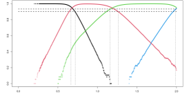
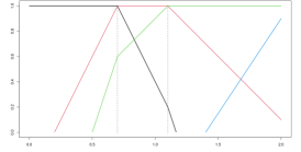
Figure 6. Illustration of Proposition 4.7, where $\Psi=((0.2,2),(0.5,3),(1.4,1.5))$. Left: Moran model with birth times and increments corresponding to $\Psi$, $B^{N}_{i}=1$ for $i=1,2,3$, $N=500\,000$; horizontals: $1-\frac{\log\log N}{2\log N}$ resp. $\overline{h}_{N}=1-\frac{\log\log N}{3\log N}$; verticals mark $\tau_{1}^{N},\sigma_{1}^{N},\tau_{2}^{N},\sigma_{2}^{N},\tau_{3}^{N}$ from left to right. Right: $\mathbb{H}(((1,0)),\Psi)$, dotted verticals give $\tau_{1}$ and $\tau_{2}$ respectively.

The following asymptotic description of a selective sweep in the 2-type Moran model under logarithmic scaling is a straightforward consequence of Proposition 4.7 with $k=2$.

Corollary 4.8 (Full sweep with two types).

For $N\in\mathbb{N}$, $m_{1}:=0$, $m_{2}:=s>0$, let $X^{N}=(X_{1}^{N},X_{2}^{N})$ be the Markov process on ${\mathcal{S}}_{N}^{2}$ started at $X^{N}(0)=(N-1,1)$ with generator (4.2) (where $k:=2$). Again, let $H^{N}_{\ell}$ be defined by (4.3), and let

$$h_{1}(t):=((2-st)\wedge 1)^{+}=\begin{cases}1&\text{if }t\in[0,\frac{1}{s}),\\ 1-s(t-\frac{1}{s})&\text{if }t\in[\frac{1}{s},\frac{2}{s}),\\ 0&\text{if }t\geq\frac{2}{s},\end{cases}\quad\quad h_{2}(t)=st\wedge 1.$$

Then, there is a sequence of events $E_{N}$ with probabilities tending to $\frac{s}{1+s}$ as $N\to\infty$ such that the following convergences hold in probability, uniformly in $t$ in compact subsets of $[0,\infty)$,

1. $\displaystyle\big{|}H_{1}^{N}(t)-({\mathchoice{1\mskip-4.0mu\mathrm{l}}{1\mskip-4.0mu\mathrm{l}}{1\mskip-4.5mu\mathrm{l}}{1\mskip-5.0mu\mathrm{l}}}_{E_{N}^{c}}+{\mathchoice{1\mskip-4.0mu\mathrm{l}}{1\mskip-4.0mu\mathrm{l}}{1\mskip-4.5mu\mathrm{l}}{1\mskip-5.0mu\mathrm{l}}}_{E_{N}}h_{1}(t))\big{|}\xrightarrow{N\to\infty}0.$

2. $\displaystyle\big{|}H_{2}^{N}(t)-{\mathchoice{1\mskip-4.0mu\mathrm{l}}{1\mskip-4.0mu\mathrm{l}}{1\mskip-4.5mu\mathrm{l}}{1\mskip-5.0mu\mathrm{l}}}_{E_{N}}h_{2}(t)\big{|}\xrightarrow{N\to\infty}0.$

4.4. Adding one new mutation

Let $X_{1}^{N},\ldots,X_{k}^{N}$ be as in Proposition 4.7. Let $T$ be Exp$(\lambda)$-distributed and $A$ have distribution $\gamma$. Assume that $T$ and $A$ are independent of each other and of everything else. At time $T$, choose an individual uniformly at random from the Moran$(N)$-population and add the value $A$ to its fitness. Denoting the index of the family of the randomly picked individual by $\Lambda_{N}$ and assigning the index $k+1$ to a new family founded by this individual, we thus have a process $\widetilde{X}^{N}$ which up to time $T-$ coincides with $X^{N}$ and whose state at time $T$ is defined as

$$(\widetilde{X}_{1}^{N}(T),\ldots,\widetilde{X}_{\Lambda_{N}}^{N}(T),\ldots,\widetilde{X}_{k}^{N}(T)):=(X_{1}^{N}(T-),\ldots,X_{\Lambda_{N}}^{N}(T-)-1,\ldots,X_{k}^{N}(T-)),$$

$$\widetilde{X}_{k+1}^{N}(T):=1,\quad M^{N}_{k+1}:=m_{\Lambda_{N}}+A.$$

For $t\geq T$, let $\widetilde{X}^{N}$ follow the dynamics (4.2), with $k+1$ in place of $k$. For convenience we extend $\widetilde{X}^{N}_{k+1}$ to the entire positive time axis by setting it to be $0$ for $t<T$. Let $\widetilde{H}^{N}$ be the process of logarithmic type frequencies of $\widetilde{X}^{N}$ defined as in (4.3). Let

$$\widetilde{B}^{N}:={\mathchoice{1\mskip-4.0mu\mathrm{l}}{1\mskip-4.0mu\mathrm{l}}{1\mskip-4.5mu\mathrm{l}}{1\mskip-5.0mu\mathrm{l}}}_{\{\widetilde{X}_{k+1}^{N}(t^{N})\geq\log N\}}\quad\text{ where }\quad t^{N}=\tfrac{1}{\sqrt{\log N}},$$

and re-define the system $\widehat{H}^{N}$ from Proposition 4.7 by adding a trajectory $\widehat{H}_{k+1}^{N}$ that is $0$ for $t\leq T$, starts at time $T$ at height $0$ with slope $A\widetilde{B}^{N}$, and then interacts with the other trajectories of $\widehat{H}^{N}$ in the way described in Section 2.2. Let

$$\rho^{N}(T):={\rm argmax}\{m_{\ell}\mid 1\leq\ell\leq k\mbox{ with }\widehat{H}^{N}_{\ell}(T)=1\},$$

i.e. the index of the family which is resident at time $T$ in the PIT $\widehat{H}^{N}$.

Lemma 4.9.

With $\widetilde{H}^{N}$ denoting the logarithmic type frequencies of $\widetilde{X}^{N}$ we have as $N\to\infty$

$$\mathbb{P}(M_{k+1}^{N}=m_{\rho^{N}(T)}+A)\quad\to 1,$$ (4.30)

$$\mathbb{P}\big{(}\widetilde{B}^{N}=1\mid A\big{)}\to\frac{A}{1+A}\quad\mbox{a.s.}$$ (4.31)

$$\sup_{1\leq\ell\leq{k+1}}\sup_{0\leq t\leq t_{0}}|\widetilde{H}^{N}_{\ell}(t)-\widehat{H}_{\ell}^{N}(t)|\to 0\quad\mbox{in probability for all }t_{0}>0.$$ (4.32)

Proof.

According to properties (2)-(3) in Proposition 4.7 we have

$$\mathbb{P}(\Lambda^{N}=\rho^{N}(T))\to 1\quad\mbox{ as }N\to\infty.$$

The convergence (4.30) thus follows from the definition of $M^{N}_{k+1}$. Convergence (4.31) follows from (4.25). Finally, (4.32) follows from a twofold application of Proposition 4.7, first by restricting (4.24) to $[0,T]$ and then by applying Proposition 4.7 on the interval $[T,\infty)$ to $\widetilde{X}^{N}$ now with $k+1$ instead of $k$ types, and with the above described initial states $\widetilde{X}^{N}(T)$. ∎

4.5. Completion of the proof of Theorem 2.14

We now revert to the definition of $(\mathscr{X}^{N},\mathscr{M}^{N},\mathscr{I}^{N})$ as in Remark 2.12 in Section 2.4 . Let $H^{N}$ be as in (4.3). We define

$$B^{N}_{i}:={\mathchoice{1\mskip-4.0mu\mathrm{l}}{1\mskip-4.0mu\mathrm{l}}{1\mskip-4.5mu\mathrm{l}}{1\mskip-5.0mu\mathrm{l}}}_{\{\mathscr{X}^{N}_{i}(t^{N})\geq\log N\}}\quad\text{ where }\quad t^{N}=\tfrac{1}{\sqrt{\log N}}.$$

Let $\widehat{H}^{N}$ be the PIT with initial state $((1,0),(0,0),(0,0),\ldots)$, and with newborn trajectories born at times $T_{i}$ with initial slope $A_{i}B^{N}_{i}$. For $i=1,2,\ldots$, let $\rho^{N}(T_{i})$ be the type that is resident in $\widehat{H}^{N}$ at time $T_{i}$, i.e. that index $J<i$ for which $\widehat{H}_{J}^{N}(T_{i})=1$. (Note that by construction $\rho^{N}(T_{i})$ is a.s. well-defined.) We define recursively

$$\widehat{M}_{i}^{N}:=\widehat{M}^{N}_{\rho^{N}(T_{i})}+A_{i},\qquad\widehat{M}^{N}_{0}:=m_{0}.$$ (4.33)

We now state a “quenched” version of Theorem 2.14.

Proposition 4.10.

Conditionally given $(T_{i},A_{i})_{i\in\mathbb{N}}$, for all $i=1,2,\ldots$,

$$\sup_{0\leq\ell<i}\sup_{0\leq t\leq T_{i}}|H^{N}_{\ell}(t)-\widehat{H}_{\ell}^{N}(t)|\to 0\quad\mbox{in probability}\quad\mbox{as }N\to\infty$$ (4.34)

and

$$\mathbb{P}((M_{0}^{N},\ldots,M_{i}^{N})=(\widehat{M}_{0}^{N},\ldots,\widehat{M}_{i}^{N}))\to 1\qquad\mbox{as }N\to\infty.$$

Proof.

This follows from Lemma 4.9 by induction over $i$. ∎

For all $i=1,2,\ldots$, let $B_{i}$ be mixed Bernoulli with random parameter $\frac{A_{i}}{1+A_{i}}$, i.e.

$$\mathbb{P}(B_{i}=1\mid A_{i})=\frac{A_{i}}{1+A_{i}}.$$

Let $\mathscr{H}=(H_{i})_{i\in\mathbb{N}_{0}}$ be the PIT$(\lambda,\gamma)$ as defined in Section 2.2. For $i=1,2,\ldots$, let $\rho(T_{i})$ be the resident type in $\mathscr{H}$ at time $T_{i}$ (as defined in (2.6)), and let $M_{i}$ be defined as in (2.20).

Proposition 4.11.

For all $i=1,2,\ldots$ and all $t_{0}>0$, as $N\to\infty$,

$$(B_{1}^{N},\ldots,B_{i}^{N}) \xrightarrow{\,\,d\,\,}(B_{1},\ldots,B_{i}),$$ (4.35)

$$\big{(}\widehat{H}^{N}(t)\big{)}_{0\leq t\leq t_{0}} \xrightarrow{\,\,d\,\,}\big{(}H(t)\big{)}_{0\leq t\leq t_{0}}\,\,\mbox{\rm as random elements of }\big{(}\mathcal{D}([0,t_{0}],[0,1])\big{)}^{\mathbb{N}_{0}},$$ (4.36)

$$(\rho^{N}(T_{1}),\ldots,\rho^{N}(T_{i})) \xrightarrow{\,\,d\,\,}(\rho(T_{1}),\ldots,\rho(T_{i})),$$ (4.37)

$$(\widehat{M}_{0}^{N},\ldots,\widehat{M}_{i}^{N}) \xrightarrow{\,\,d\,\,}(M_{0},\ldots,M_{i}).$$ (4.38)

Moreover, for each $i$ the above convergences occur jointly.

Proof.

(4.35) follows by induction from (4.31). The convergence (4.36) is a consequence of (4.35) and the definitions of $H$ and $\widehat{H}^{N}$. The convergence (4.37) follows from (4.35) together with the construction of the PIT and the fact that the $T_{i}$ have a continuous distribution. Finally, (4.38) results from (4.37) together with the update rules (2.20) and (4.33). ∎

Combining Proposition 4.10 with (4.36) and (4.38) gives the assertion of Theorem 2.14.

Before proving Proposition 2.15, note that the average fitness at times of a resident change can take any value between the fitness of the former and the fitness of the new resident. Consequently, in contrast to Proposition 4.11, we restrict Proposition 2.15 to the $M_{2}$-topology.

4.6. Proof of Proposition 2.15

Denote by $\rho(t)$ the resident in the system

$$\mathbb{H}((1,0),((T_{i},A_{i}))_{i})$$

at time $t$ and let $t$ not be a resident change time. Then (4.36) implies that with (quenched) probability tending to $1$

$$\Big{(}1-\frac{1}{\log N}\Big{)}M^{N}_{\rho(t)}\leq\overline{F}^{N}(t)\leq M^{N}_{\rho(t)}+\frac{1}{\log N}\max_{i\leq\mathscr{I}^{N}(t)}M^{N}_{i}.$$

That is, conditionally given $(T_{i},A_{i})_{i}$, $d_{M_{1}}(\overline{F}^{N},\widehat{F}^{N})\to 0$ in probability, where $\widehat{F}^{N}$ denotes the resident fitness in the PIT$((1,0),\beth^{N})$ with $\beth^{N}:=(T_{i},A_{i}B_{i}^{N})_{i}$. Further, by Proposition 4.11, $\widehat{F}^{N}\xrightarrow{d}F$ with respect to the Skorokhod $J_{1}$-topology, which is stronger than the $M_{2}$-topology. The desired convergence thus holds, conditionally given $(T_{i},A_{i})_{i}$. Finally, by triangular inequality and dominated convergence,

$$d_{M_{2}}(\overline{F}^{N},F)\to 0$$

in probability, without conditioning.∎

4.7. General initial conditions

In Section 2.2 we only defined the process $\mathscr{H}=\mathbb{H}(((1,0)),\Psi)$ with a homogeneous initial condition where at time zero, only one trajectory is present, namely the one of the initial resident, which starts at height 1. This corresponds to the initial condition $\mathcal{X}^{N}(0)=(N,0,0,\ldots)$ for the prelimiting Moran model that we considered in Theorem 2.14. This simplification solely comes from the fact that arbitrary initial conditions would complicate the notation of Theorem 2.14 and necessitate further discussion, which we decided to omit for the reader’s comfort.

However, Proposition 4.7 makes clear that Theorem 2.14 also holds for quite arbitrary initial conditions – at least those satisfying its conditions. (Note that not all such initial conditions can be reached via starting from the homogeneous initial condition and following the dynamics of the PIT.) Further, a simple modification of the renewal argument used in proof of Theorem 2.8 implies that the first positive time when there is a unique trajectory with height 1 and slope 0 and all other trajectories are at height 0 is stochastically dominated by a geometric random variable whose parameter is positive and does not depend on the initial condition. This way, starting with a single type at time 0 is not restrictive, and the speed of adaptation $\overline{v}$ will not depend on the choice of the initial condition either.

4.8. General type space

Instead of understanding a type in terms of its fitness and time of arrival, one could think of types in a more abstract manner, i.e. as elements of a (measurable) type space $(\Theta,{\mathcal{A}})$. Mutation occurring in an individual $i$ would then assign a new (random) type $\vartheta_{i}$ to it, distributed as $\mu(\vartheta_{j},\cdot)$, where $\vartheta_{j}$ is type of parent individual $j$ and $\mu:\Theta\times{\mathcal{A}}\to[0,1]$ is a probability kernel. Then, between mutations, the evolution of the clonal subpopulations in the corresponding generalized Moran model could be described by the generator

$$Lf(x)=\frac{1}{N}\sum_{i\neq j}x_{i}x_{j}(1+c(\vartheta_{i},\vartheta_{j})^{+})(f(x+e_{i}-e_{j})-f(x)),$$

where $c\in\mathbb{R}^{\Theta\times\Theta}$ can be viewed as a competition matrix. (Note that taking $\Theta=[0,\infty)$, $\mu(\theta,\cdot)=\delta_{\theta}\ast\gamma$ and $c(\theta,\vartheta)=\theta-\vartheta$ recovers the Moran model in Section 2.4.) It is conceivable that this generalized model might be used to incorporate slowdown effects that produce strict concavity in population fitness as observed in the Lenski experiment (see Fig. 2 in [WRL13]).

We postulate that with similar methods based on Lemmas 4.4 and 4.5 one should arrive at a corresponding scaling limit result – possibly even when allowing $c$ to vary over time. However, the coupling used for the quenched convergence result would have to become much more involved. Also, in the limiting system new challenges might arise, such as cyclic effects providing infinitely many resident changes from finitely many mutations, possibly even in finite time; similarly to [BPT23, Examples 3.2, 3.5 and 3.6] and [CKS21, Example 3.6]; Figure 7 for an illustration.

Figure 7. Illustration of cyclicity. In each case, $\Theta=\{0,{\color[rgb]{.75,.5,.25}1},{\color[rgb]{0,0,1}2}\}$, $h_{0}(0)=1,h_{\color[rgb]{.75,.5,.25}1}(0)=1$, $h_{\color[rgb]{0,0,1}2}(0)=\frac{1}{2}$. Left: $c({\color[rgb]{.75,.5,.25}1},0)=c({\color[rgb]{0,0,1}2},{\color[rgb]{.75,.5,.25}1})=c(0,{\color[rgb]{0,0,1}2})=1$. Mid: $c({\color[rgb]{.75,.5,.25}1},0)=0.5,c({\color[rgb]{0,0,1}2},{\color[rgb]{.75,.5,.25}1})=1,c(0,{\color[rgb]{0,0,1}2})=1.5$. Right: $c(t,{\color[rgb]{.75,.5,.25}1},0)=c(t,{\color[rgb]{0,0,1}2},{\color[rgb]{.75,.5,.25}1})=c(t,0,{\color[rgb]{0,0,1}2})=2^{-\lfloor\log_{2}(2-t)\rfloor}{\mathchoice{1\mskip-4.0mu\mathrm{l}}{1\mskip-4.0mu\mathrm{l}}{1\mskip-4.5mu\mathrm{l}}{1\mskip-5.0mu\mathrm{l}}}_{\{t<2\}}$.

4.9. Non-Poissonian birth times

In fact, Theorem 2.14 and its “quenched” version, Proposition 4.10 remain true when $(T_{i})_{i\in\mathbb{N}}$ is not a Poisson process but an arbitrary renewal process such that the i.i.d. increments $T_{i}-T_{i-1}$ are a.s. strictly positive and have a continuous distribution function. Indeed, it can be observed in Section 4.4 that the fact that $T$ is exponentially distributed plays no particular role there. The assertions of Lemma 4.9 also hold with $T$ being any strictly positive random variable with a continuous distribution function, where the latter condition is necessary in order to guarantee that $T$ typically lies in one of the intervals where the resident is well-defined, i.e. $(\sigma_{i}^{N},\tau_{i+1}^{N})$ in the notation of Proposition 4.7. Under the same continuity assumption on $T_{i}-T_{i-1}$ for $i\geq 1$ (where $T_{0}=0$), which was also used in the proof of Proposition 4.11, one can verify all the results of Section 4.5 analogously to the Poissonian case.

A generalization of our proof techniques on the speed of adaptation however requires further assumptions. In the proof of Lemma 3.5 we used that if a sufficiently fit mutant has a sufficiently large time interval before as well as after its birth time during which no other contender is born, then the type of this mutant will become resident after a limited amount of time, via a solitary resident change. But for example, if the inter-arrival times $T_{i}-T_{i-1}$ of the renewal process $(T_{i})_{i\in\mathbb{N}}$ are bounded from above and the supremum of the support of $\gamma$ is comparably very low, then it may happen that no mutation can become resident before another mutant is born, i.e. no resident change can be solitary. We nevertheless expect that even in such a case, Theorem 2.8 should remain true, but we defer the investigation of such questions to future work.

5. Discussion and outlook

5.1. The case of non-strong selection

In mathematical population genetics weak selection classically refers to the scaling regime where fitness increments are of the order of $1/N$. In contrast, as we already mentioned, strong selection means that $s=s_{N}$ does not scale with $N$. In the latter regime, in the proof of Theorem 2.14, we exploited that the frequency of all mutations, including non-contending ones, arising in finite time stays finite in the scaling limit. This is never true for $s_{N}\to 0$ as $N\to\infty$; then only an asymptotically vanishing fraction $\Theta(s_{N})$ of mutants survives drift. This makes the analysis more involved since then the supercriticality of the branching processes that approximate the clonal subpopulations tends to $0$ as $N\to\infty$.

One interesting regime is that of moderate selection, where $s_{N}\asymp N^{-b}$ for some $0<b<1$. Recent results show that Haldane’s formula for the survival probability of a mutant applies not only in Moran models but also in Cannings models for the case of moderately weak selection ($s_{N}\asymp N^{-b}$, $\tfrac{1}{2}<b<1$) ([BGCPW21b]) as well as for the case of moderately strong selection ($s_{N}\asymp N^{-b}$, $0<b<\tfrac{1}{2}$) ([BGCPW21a]). Simulations indicate that moderate selection yields a similar limiting process as the PIT, however, piecewise linear trajectories now start and end at height $b$ instead of $0$. That is, we conjecture that contending mutant subpopulations reach size $N^{b}$ in $o(s_{N}^{-1}\log N)$ time and decaying subpopulations of size $o(N^{b})$ go extinct in $o(s_{N}^{-1}\log N)$ time, see Figure 8.

The regime that is intermediate between moderate and strong selection, where $s_{N}$ tends to zero as a slowly varying function of $N$, is also interesting to study. In this regime a contender who ever becomes resident takes a time $\Theta(s_{N}^{-1}\log N)$ to reach residency. Thus, altogether we expect that in this regime time has to be sped up by a factor of $s_{N}^{-1}\log N$ rather than by $\log N$ to obtain a limiting process similar to the PIT (whose trajectories do not have jumps). We also see that the mutation regime where waiting times between consecutive contending mutations and lengths of selective sweeps are of the same order should be still $\mu_{N}\asymp 1/\log N$.

We defer the precise investigation of these regimes to future work.

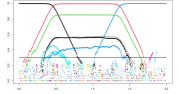
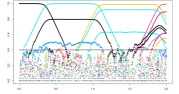
Figure 8. Simulation of a Cannings model with mutation and selection, $N\approx 2.1\cdot 10^{9}$, under moderate selection, i.e. $s_{N}=N^{-b}$, on timescale $N^{b}\log N$. Left: $b=0.2$, middle: $b=0.3$, right: $b=0.4$, each indicated by horizontal line.

5.2. Mutation rates outside the GL-regime

Let us compare our results to prior work in population genetics (with a constant population size) and population dynamics (with logistic competition) in other mutation frequency regimes. The Gerrish–Lenski regime $\mu_{N}\asymp\frac{1}{\log N}$ is between the so-called rare mutation regime ($\mu_{N}\ll\frac{1}{\log N}$) and the polynomial one ($\mu_{N}\asymp N^{\alpha}$, $\alpha\in(0,1]$). We have seen that in the Gerrish–Lenski regime most of the time there is a unique resident subpopulation and typically only residents suffer mutations.

If mutations are rare and selection is strong, the waiting times between the births of two consecutive mutants are of order $\mu_{N}^{-1}$ $\gg\log N$, while selective sweeps take time of order $\log N$. Hence, clonal interference plays asymptotically no role as $N\to\infty$. If mutations are all beneficial and the long-term macroscopic coexistence of different sub-populations is excluded (like in our model), then with high probability, every mutant will either fix or go extinct before the next mutant arrives. The same behaviour applies in the case of logistic competition, where one additionally needs to assume that $\mu_{N}\gg{\rm e}^{-VN}$ for all $V>0$ to avoid extinction of the population before the appearance of the first mutant. See the seminal paper by Champagnat [Cha06] and the references therein. Selective sweeps in population-genetic models were already studied earlier, see e.g. [KHL89, DS04]. Scaling time by the mutation rate, the durations of selective sweeps vanish, and the process of the fitness of the population converges to a pure jump process called the trait substitution sequence of adaptive dynamics, as it was shown in [Cha06]. The case where coexistence is possible was first studied in [CM11].

A rare mutation regime with $\mu_{N}\sim N^{-a}$ and $s_{N}\sim N^{-b}$ was considered in [GCKWY16]; there, conditions were imposed on $a$ and $b$ that guarantee that w.h.p. as $N\to\infty$ no more than one mutant family is present in the population except the resident type. In particular, these conditions implied that the times at which a new resident is established converge to a homogeneous Poisson process on the time scale whose unit is $(\mu_{N}s_{N})^{-1}$ generations. Recently, in [US24] it was shown that this same converge remains true in the rare mutation regime $\mu_{N}=o\big{(}\frac{1}{\log N}\big{)}$ for $s_{N}\sim N^{-b}$ with any $0<b<1$, even though then at any time a number of (small) mutant families is around that diverges as $N\to\infty$.

In the polynomial (a.k.a. power-law) mutation regime, there is a constant flow of repeated mutations, even between mesoscopic (size $\Theta(N^{\beta})$, $\beta<1$) subpopulations. This wipes out random genetic drift entirely as $N\to\infty$, so that the scaling limit of logarithmic subpopulation sizes is still piecewise linear but deterministic. As already mentioned, the convergence to such a process was first verified by Durrett and Mayberry [DM11] in a population-genetic context. The analogous mutation regime has been studied in various models of adaptive dynamics [BCS19, CMT21, CKS21, EK21, BPT23, Pau23, EK23] and branching processes [Bro24]. These models typically come with a fixed mutation graph; the possible types/traits of individuals form a countable (often finite) set, and mutations between some of these types are possible. The scaling limit does not feature clear parent$\to$child relations anymore since mutations do not appear as a point process but rather as a piecewise constant influx.

A two-type model with logistic competition and with back-and-forth mutations between a wildtype and a strongly beneficial type was studied in [Sma17] for various mutation regimes, including the regime analogous to $\mu_{N}\asymp 1$.

5.3. The continued lines representation.

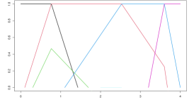
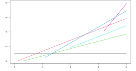
Figure 9. Left: $\mathbb{H}(((1,0)),((0.1,1.5),(0.3,1),(1.1,0.7),(2,0),(3.2,2.5)))$, right: corresponding system of continued lines.

To simulate the PIT, one needs to know the extinction time of all trajectories of contending mutations and their slope at all resident changes between their birth and extinction, even though only increasing subpopulations affect the future of other subpopulations. There is an equivalent representation of this process which can be simulated without any computations involving already decaying height functions, which may be useful for future algorithmic investigations. We call this the continued lines representation and describe it as follows.

At any time $t\geq 0$ we consider a finite family of half-lines $\{L_{0},L_{1},\ldots,L_{k}\}$ infinite towards the right, where $L_{0}$ is the constant 1 half-line starting at time 0, and we denote by $L^{r}(t)=\max\{L_{1}(t),\ldots,L_{k}(t)\}$ the pointwise maximum, namely the resident line, with $F(t)$ denoting its slope at time $t$. As the Poisson point process delivers a new point $(T_{k+1},A_{k+1})$, we add a line $L_{k+1}$ to the system starting at $L^{r}(T_{k+1})-1$ with slope $F(T_{k+1})+A_{k+1}B_{k+1}$. Notably, this gives an alternative construction of $\mathscr{H}$ as for any $k$, $H_{k}(t)=L_{k}(t)-(L^{r}(t)-1)$. After $T_{k}$, the $k$-th type goes extinct as soon as $H_{k}(t)$ reaches $L^{r}(t)-1$ again (which happens immediately at time $T_{k}$ if $B_{k}=0$). See Figure 9 for an illustration.

Appendix A A functional CLT for renewal reward processes

In this section we provide a functional central limit theorem for renewal reward processes, thus completing the proof of Theorem 2.11 that was given in Section 3.4.

Let $(X_{n},\tau_{n})$, $n\in\mathbb{N}$, be an i.i.d. sequence of $\mathbb{R}\times(0,\infty)$-valued random variables. We assume that $X_{1}$ and $\tau_{1}$ are both square-integrable. Define

$$T_{n}:=\tau_{1}+\cdots+\tau_{n},\qquad S_{n}=X_{1}+\cdots+X_{n},$$

and set

$$N_{t}:=\sup\{n\in\mathbb{N}\colon\,T_{n}\leq t\},\qquad Z_{t}:=S_{N_{t}},$$

where in the above we take $\sup\varnothing=0$. By the SLLN for sums of i.i.d. random variables,

$$\lim_{n\to\infty}\frac{T_{n}}{n}=\mathbb{E}[\tau_{1}]=:\theta\quad\text{ and }\quad\lim_{n\to\infty}\frac{S_{n}}{n}=\mathbb{E}[X_{1}]=:\mu\quad\text{almost surely,}$$

and an interpolation argument shows that (see e.g. [EKM97, Theorems 2.5.10 and 2.5.14]),

$$\lim_{t\to\infty}\frac{N_{t}}{t}=\frac{1}{\theta}\quad\text{ and }\quad\lim_{t\to\infty}\frac{Z_{t}}{t}=\frac{\mu}{\theta}=:v\quad\text{almost surely.}$$

Here we will prove a functional central limit theorem for $Z_{t}$, as stated next.

Theorem A.1.

Assume that $\sigma:=\sqrt{\mathbb{E}[(X_{1}-v\tau_{1})^{2}]/\theta}>0$. Then

$$\Big{(}\frac{Z_{nt}-nv}{\sigma\sqrt{n}}\Big{)}_{t\geq 0}\quad\overset{d}{\longrightarrow}\quad W$$

where $W=(W_{t})_{t\geq 0}$ is a standard Brownian motion and “$\overset{d}{\longrightarrow}$” denotes convergence in distribution as $n\to\infty$ in the space of càdlàg functions from $[0,\infty)$ to $\mathbb{R}$ equipped with the Skorokhod $J_{1}$-topology.

Proof.

We adapt the proof of Theorem 1.4(b) in [dHHdS⁺15]. First note that, by the Donsker-Prokhorov invariance principle for sums of i.i.d. random variables,

$$\widehat{W}^{(n)}=\big{(}\widehat{W}^{(n)}_{t}\big{)}_{t\geq 0}:=\Bigg{(}\frac{1}{\sigma\sqrt{\theta}\sqrt{n}}\sum_{k=1}^{\lfloor nt\rfloor}(X_{k}-v\tau_{k})\Bigg{)}_{t\geq 0}\overset{d}{\longrightarrow}W.$$

Consider the random time change $\varphi_{n}(t):=N_{nt}/n$. Let us show that

$$\lim_{n\to\infty}\sup_{t\in[0,M]}\Big{|}\varphi_{n}(t)-\frac{t}{\theta}\Big{|}=0\quad\text{in probability for any $M>0$.}$$ (A.1)

Indeed, since $T_{n}>t$ if and only if $N_{t}<n$, given $\delta,\varepsilon>0$, there are $\delta^{\prime},\varepsilon^{\prime}>0$ such that, for large $n$,

$$\mathbb{P}\Bigg{(}\sup_{t\in[\delta,\infty)}\Big{|}\frac{\varphi_{n}(t)}{t}-\frac{1}{\theta}\Big{|}>\varepsilon\Bigg{)}\leq\mathbb{P}\big{(}\exists k\geq\delta^{\prime}n\colon\,|T_{k}/k-\theta|\geq\varepsilon^{\prime}\big{)}\underset{n\to\infty}{\longrightarrow}0$$

by the SLLN for $T_{n}$. On the other hand, taking $\delta<\varepsilon/(2\theta)$, we obtain $\varepsilon^{\prime\prime}>0$ such that

$$\mathbb{P}\Big{(}\sup_{t\in[0,\delta]}\Big{|}\varphi_{n}(t)-\frac{t}{\theta}\Big{|}>\varepsilon\Big{)}\leq\mathbb{P}\Big{(}\frac{N_{n\delta}}{n\delta}\geq\frac{1}{\theta}+\varepsilon^{\prime\prime}\Big{)},$$

and the r.h.s. again converges to $0$ as $n\to\infty$ by the SLLN for $N_{t}$. This shows (A.1). In particular, $\varphi_{n}$ converges in probability with respect to the Skorokhod topology to the linear function $t\mapsto t/\theta$. Using a time-change argument as in Section 17 of [Bil68] (see in particular (17.7)–(17.9) and Theorem 4.4 therein), we conclude that $t\mapsto\widehat{W}^{(n)}_{\varphi_{n}(t)}$ converges to a Brownian motion time-changed by $t\mapsto t/\theta$, or equivalently, to a Brownian motion multiplied by $1/\sqrt{\theta}$. To compare with $Z_{t}$, note that

$$\Big{|}\frac{Z_{nt}-ntv}{\sigma\sqrt{n}}-\sqrt{\theta}\widehat{W}^{(n)}_{\varphi_{n}(t)}\Big{|}=\frac{|v|}{\sigma}\cdot\frac{|T_{N_{nt}}-nt|}{\sqrt{n}}\leq\frac{|v|}{\sigma}\cdot\frac{T_{N_{nt}+1}-T_{N_{nt}}}{\sqrt{n}}$$

so that, for any $M,\varepsilon>0$, there is an $\varepsilon^{\prime}>0$ such that

$$\mathbb{P}\Bigg{(} \sup_{t\in[0,M]}\Big{|}\frac{Z_{nt}-ntv}{\sigma\sqrt{n}}-\sqrt{\theta}\widehat{W}^{(n)}_{\varphi_{n}(t)}\Big{|}\geq\varepsilon\Bigg{)}$$

$$\leq\mathbb{P}(N_{nM}>2nM/\theta)+\mathbb{P}\big{(}\exists k\leq 2nM/\theta+1\colon\,\tau_{k}\geq\varepsilon^{\prime}\sqrt{n}\big{)}$$

$$\leq\mathbb{P}(N_{nM}>2nM/\theta)+(2nM/\theta+1)\mathbb{P}(\tau_{1}\geq\varepsilon^{\prime}\sqrt{n}).$$

The first term above converges to $0$ as $n\to\infty$ by the LLN for $N_{t}$, while the second converges to $0$ since $\tau_{1}$ is square-integrable. This shows that the Skorokhod distance between $\sqrt{\theta}\widehat{W}^{(n)}_{\varphi_{n}(t)}$ and $(Z_{nt}-ntv)/(\sigma\sqrt{n})$ converges to zero in probability, concluding the proof. ∎

Appendix B Stochastic domination

In this section we provide the couplings required in the proofs of Lemmas 4.3,4.4 and 4.5, combining results from [KKO77] and [Mas87]. Since we feel that these arguments are of independent interest, we state and prove, for two Markov chains $X$, $Y$ in continuous time, a comparison result in terms of an ordered coupling between $Y$ and the mapped process $(\varphi(X_{t}))_{t\geq 0}$ under the assumption of a “monotone intertwining” of $\varphi$ and the jump rates of $X$ and $Y$.

Specifically, let $E,F$ be countable sets, $F$ equipped with a partial order $\leq$, and let $\varphi:E\to F$. Let $X=(X_{t})_{t\geq 0}$, $Y=(Y_{t})_{t\geq 0}$ be continuous-time càdlàg Markov jump processes on $E,F$ with bounded generators $A,B$, respectively. Here we will say that $Y$ is monotone if, for any bounded non-decreasing $g:F\to\mathbb{R}$, $Bg$ is also non-decreasing. We will write $\mathbb{P}^{X}_{x}$ for the law of $X$ started from $x$, $\mathbb{E}^{X}_{x}$ for the corresponding expectation, and analogously for $Y$.

Theorem B.1.

Assume that $Y$ is monotone and that, for all bounded non-decreasing $g:F\to\mathbb{R}$,

$$A(g\circ\varphi)(x)\leq Bg(\varphi(x))\quad\forall x\in E_{0}$$ (B.1)

where $E_{0}\subset E$. Denote by $\tau_{0}:=\inf\{t\geq 0\colon\,X_{t}\notin E_{0}\}$ the first time when $X$ exits $E_{0}$. Then, for all $x\in E_{0}$ and $y\in F$ with $\varphi(x)\leq y$, there exists a coupling $Q$ of $(\varphi(X_{t}))_{t\geq 0}$ under $\mathbb{P}^{X}_{x}$ and of $Y$ under $\mathbb{P}^{Y}_{y}$ such that $Q(\varphi(X_{t})\leq Y_{t}\,\,\forall t\in[0,\tau_{0}])=1,$ where we interpret $[0,\infty]=[0,\infty)$. The analogous result holds with the inequalities reversed.

Proof.

We will only prove the theorem for the inequalities as first stated; the proof for the reversed inequalities is analogous.

Let us first reduce to the case $E_{0}=E$. If $E_{0}\subsetneq E$, let $A(x,y)$ denote the matrix entries corresponding to the operator $A$. If $\varphi$ is not surjective, we enlarge $E$ to $\widehat{E}:=E\cup(F\setminus\varphi(E))$ where the union is disjoint, and extend $\varphi$ to $\widehat{E}$ by setting $\varphi(x)=x$ for $x\notin E$. Define $\widehat{X}$ to be the Markov jump process on $\widehat{E}$ with generator $\widehat{A}$ given by $\widehat{A}(x,y)=A(x,y){\mathchoice{1\mskip-4.0mu\mathrm{l}}{1\mskip-4.0mu\mathrm{l}}{1\mskip-4.5mu\mathrm{l}}{1\mskip-5.0mu\mathrm{l}}}_{E}(y)$ if $x\in E_{0}$, and $\widehat{A}(x,y)=B(\varphi(x),\varphi(y))/\#\varphi^{-1}(\varphi(y))$ otherwise. One may verify that (B.1) is valid for $\widehat{A}$ in place of $A$ and all $x\in\widehat{E}$, and it is clear that $X$ and $\widehat{X}$ are equal in distribution up to their first exit of $E_{0}$.

From here on we assume $E_{0}=E$, implying $\tau_{0}=\infty$. In this case, the first step is to use [Mas87, Theorem 3.5] (with the strong stochastic ordering; see Definition 2.4 therein) to conclude that, for any $t>0$ and any $x\in E$, $y\in F$ with $\varphi(x)\leq y$,

$$\varphi(X_{t}) \mathbb{P}^{X}_{x} Y_{t} \mathbb{P}^{Y}_{y}$$ under is stochastically dominated by under . (B.2)

First of all, note that our assumptions on $Y$ imply that its generator $B$ is monotone in the sense discussed in Definition 3.2 in [Mas87], i.e., for any $t>0$ and $y_{1}\leq y_{2}\in F$,

$$Y_{t} \mathbb{P}^{Y}_{y_{1}} Y_{t} \mathbb{P}^{Y}_{y_{2}}$$ under is stochastically dominated by under . (B.3)

Indeed, this follows from [Lig85, Theorem 2.2] and the fact that the semigroup for $Y$, $\exp(tB)$, has e.g. the representation given right before Definition 3.2 in [Mas87]. To verify that our assumptions imply those of Theorem 3.5 in [Mas87], note first that $f$, $E^{\prime}$, $E$ therein correspond to our $\varphi$, $E$, $F$, respectively. Then note that the mapping $\Phi(\varphi)$ from $\ell_{1}(E)$ to $\ell_{1}(F)$ defined before Theorem 3.5 acts by multiplication to the left. Its adjoint mapping of multiplication to the right (from $\ell_{\infty}(F)$ to $\ell_{\infty}(E)$) is defined such that $u\Phi(\varphi)\cdot v=u\cdot\Phi(\varphi)v$, i.e., $\Phi(\varphi)v(x):=\mathrm{e}_{x}\Phi(\varphi)\cdot v=v(\varphi(x))$, where $\mathrm{e}_{x}$ is the indicator function of $\{x\}$, $x\in E$. Finally, note that, according to the ordering $\leq_{\rm{st}}$ (cf. Definition 2.4 and Proposition 3.1 therein), $A\Phi(\varphi)\leq_{\rm{st}}\Phi(\varphi)B$ if and only if $A\Phi(\varphi){\mathchoice{1\mskip-4.0mu\mathrm{l}}{1\mskip-4.0mu\mathrm{l}}{1\mskip-4.5mu\mathrm{l}}{1\mskip-5.0mu\mathrm{l}}}_{\Gamma}(x)\leq\Phi(\varphi)B{\mathchoice{1\mskip-4.0mu\mathrm{l}}{1\mskip-4.0mu\mathrm{l}}{1\mskip-4.5mu\mathrm{l}}{1\mskip-5.0mu\mathrm{l}}}_{\Gamma}(x)$ for all $x\in E$ and all increasing sets $\Gamma\subset F$; since in this case ${\mathchoice{1\mskip-4.0mu\mathrm{l}}{1\mskip-4.0mu\mathrm{l}}{1\mskip-4.5mu\mathrm{l}}{1\mskip-5.0mu\mathrm{l}}}_{\Gamma}$ is non-decreasing, this follows from (B.1) (and is actually equivalent to it).

To finish the proof, we will verify the conditions of [KKO77, Theorem 4]. We write $Z=(Z_{t})_{t\geq 0}$ with $Z_{t}:=\varphi(X_{t})$. For $n\geq 2$, $t^{n}=(t_{1},\ldots,t_{n})\in[0,\infty)^{n}$ with $t_{1}<\cdots<t_{n}$ and $z^{n-1}=(z_{1},\ldots,z_{n-1})\in F^{n-1}$, define the kernel

$$p_{t^{n}}(z^{n-1},B)=\mathbb{P}^{X}_{x}(Z_{t_{n}}\in B\mid\cap_{i=1}^{n-1}\{Z_{t_{i}}=z_{i}\}),\quad B\subset F,$$

and let $q_{t^{n}}(y^{n-1},B)$ denote the analogous kernel for $Y$ in place of $Z$. The conditions of [KKO77, Theorem 4] will be verified if we show that, for any $t^{n}$, $z^{n-1}$, any $y^{n-1}$ with $z_{i}\leq y_{i}$ for $1\leq i\leq n-1$, and any non-decreasing $g:F\to\mathbb{R}$,

$$\int g(u)p_{t^{n}}(z^{n-1},du)\leq\int g(u)q_{t^{n}}(y^{n-1},du).$$ (B.4)

To this end, note first that, since $Y$ is Markovian,

$$\int g(u)q_{t^{n}}(y^{n-1},du)=\mathbb{E}^{Y}_{y_{n-1}}[g(Y_{s_{n}})]$$ (B.5)

where $s_{n}:=t_{n}-t_{n-1}$. On the other hand, by the Markov property,

$$\mathbb{E}^{X}_{x}\big{[}{\mathchoice{1\mskip-4.0mu\mathrm{l}}{1\mskip-4.0mu\mathrm{l}}{1\mskip-4.5mu\mathrm{l}}{1\mskip-5.0mu\mathrm{l}}}_{\cap_{i=1}^{n-1}\{Z_{t_{i}}=z_{i}\}}g(Z_{t_{n}})\big{]} =\mathbb{E}^{X}_{x}\big{[}{\mathchoice{1\mskip-4.0mu\mathrm{l}}{1\mskip-4.0mu\mathrm{l}}{1\mskip-4.5mu\mathrm{l}}{1\mskip-5.0mu\mathrm{l}}}_{\cap_{i=1}^{n-1}\{Z_{t_{i}}=z_{i}\}}\mathbb{E}^{X}_{X_{t_{n-1}}}[g(Z_{s_{n}})]\big{]}$$

$$\leq\mathbb{P}^{X}_{x}\big{(}\cap_{i=1}^{n-1}\{Z_{t_{i}}=z_{i}\}\big{)}\mathbb{E}^{Y}_{z_{n-1}}\big{[}g(Y_{s_{n}})\big{]}$$

$$\leq\mathbb{P}^{X}_{x}\big{(}\cap_{i=1}^{n-1}\{Z_{t_{i}}=z_{i}\}\big{)}\mathbb{E}^{Y}_{y_{n-1}}\big{[}g(Y_{s_{n}})\big{]},$$

where for the first inequality we used (B.2) at time $s_{n}$ and for the second inequality we used (B.3). Together with (B.5), this shows (B.4). To conclude, note that the kernels $p$, $q$ plus the initial states determine all finite-dimensional distributions of $Z$, $Y$, and thus completely characterize their distributions in Skorokhod space (see e.g. [Bil68, Section 14]). Thus the construction in [KKO77, Theorem 4] provides the desired coupling. ∎

Appendix C Supercritical branching

In this section we consider a continuous-time binary Galton-Watson process $Z=(Z_{t})_{t\geq 0}$ with individual birth and death rates $b\geq 0$, $d\geq 0$ respectively, satisfying $s:=b-d>0$. We denote by $\mathbb{P}_{z}$ the law of $Z$ started at $z$, and we abbreviate $\{Z\not\to 0\}:=\{Z_{t}\geq 1,\forall t\geq 0\}$, $\{Z\to 0\}:=\{Z\not\to 0\}^{c}$.

Theorem C.1.

Let $Z$ be as above. Then:

1. For $z\in\mathbb{N}$, $\mathbb{P}_{z}(Z\not\to 0)=1-(d/b)^{z}\in(0,1]$.

2. The family of random variables $(\Xi_{z})_{z\in\mathbb{N}}$ given by

   $$\Xi_{z}:=\sup_{t\geq 0}\big{|}\log^{+}(Z_{t})-(\log z+st){\mathchoice{1\mskip-4.0mu\mathrm{l}}{1\mskip-4.0mu\mathrm{l}}{1\mskip-4.5mu\mathrm{l}}{1\mskip-5.0mu\mathrm{l}}}_{\{Z\not\to 0\}}\big{|}\quad\text{under}\quad\mathbb{P}_{z}$$

   is tight. In particular, $\mathbb{P}_{z}(\Xi_{z}<\infty)=1$ for all $z\in\mathbb{N}$. Moreover, there exists a constant $C\in(0,\infty)$ such that $\lim_{z\to\infty}\mathbb{P}_{z}(\Xi_{z}>C)=0.$

3. Let $T_{0}:=\inf\{t\geq 0\mid Z_{t}=0\}$ and, for $L>0$, $T_{L}:=\inf\{t\geq 0\mid Z_{t}\geq L\}$. Let $z_{L}\in\mathbb{N}$. Then:

   1. If $t_{L}\to\infty$ then $\mathbb{P}_{z_{L}}(T_{0}\geq t_{L})\sim\mathbb{P}_{z_{L}}(Z\not\to 0)$ as $L\to\infty$.

   2. $\mathbb{P}_{z_{L}}(T_{L}<\infty)\sim\mathbb{P}_{z_{L}}(Z\not\to 0)$ as $L\to\infty$.

   3. If $z_{L}=o(L)$ then $\lim_{L\to\infty}\frac{T_{L}}{\log(L/z_{L})}=\frac{1}{s}$ in probability under $\mathbb{P}_{z_{L}}(\cdot|Z\not\to 0)$.
      If $z_{L}\equiv 1$ this also holds almost surely.

Proof.

When $z=1$, 1) follows from [AN72, Theorem 3.4.1], and 3b) follows from the fact that $\{Z\to 0\}=\cup_{L\geq 1}\{T_{L}=\infty\}$ almost surely. It is also well-known that $(Z_{t}e^{-st})_{t\geq 0}$ is a martingale that almost-surely converges to a random variable $W$ such that $\{W>0\}=\{Z\not\to 0\}$.

For $z\geq 1$, $Z$ has the same distribution as $\sum_{k=1}^{z}Z^{(k)}$ where $Z^{(k)}$ are i.i.d. and distributed as $Z$ under $\mathbb{P}_{1}$, see e.g. [AN72, Eq. (10) on p. 105]. So $\mathbb{P}_{z}(Z\not\to 0)=1-[1-\mathbb{P}_{1}(Z\not\to 0)]^{z}$, implying 1). For 3a) and 3b), it is enough to assume that $z_{L}\to z\in\mathbb{N}$ or $z_{L}\to\infty$. If $z_{L}\to z$, note for 3b) that

$$\cap_{k=1}^{z_{L}}\{T^{(k)}_{L/z_{L}}=\infty\}\subset\{T_{L}=\infty\}\subset\{Z\to 0\}\quad\text{ almost surely,}$$

where $T^{(k)}_{L}$ is the analogue of $T_{L}$ for $Z^{(k)}$, and $\mathbb{P}_{1}(T_{L/z_{L}}=\infty)^{z_{L}}\to(d/b)^{z}$ by the case $z=1$. For 3a), note that $T_{0}=\max_{1\leq k\leq z_{L}}T^{(k)}_{0}$, so the family of distributions of $T_{0}$ under $\mathbb{P}_{z_{L}}(\cdot\mid Z\to 0)$ is tight. Thus

$$\mathbb{P}_{z_{L}}(T_{0}>t_{L})=\mathbb{P}_{z_{L}}(T_{0}>t_{L},Z\to 0)+\mathbb{P}_{z_{L}}(Z\not\to 0)\sim\mathbb{P}_{z_{L}}(Z\not\to 0)$$

since the first term after the equality converges to $0$ and the second is bounded away from $0$.

If $z_{L}\to\infty$, note for 3a) and 3b) that both $P_{z_{L}}(T_{L}<\infty)$ and $P_{z_{L}}(T_{0}>t_{L})$ are not smaller than $\mathbb{P}_{z_{L}}(Z\not\to 0)$ which converges to $1$ as $L\to\infty$.

Let us next show 2). On $\{Z\to 0\}$, $\log^{+}(\sup_{t\geq 0}Z_{t})$ is almost surely bounded. On $\{Z\not\to 0\}$,

$$\log Z_{t}-\log z-st=\log\Bigg{(}\frac{1}{z}\sum_{k=1}^{z}Z^{(k)}_{t}e^{-st}\Bigg{)}.$$ (C.1)

Now note that $\{Z\not\to 0\}=\cup_{k=1}^{z}\{Z^{(k)}\not\to 0\}$ and that, on $\{Z^{(k)}\not\to 0\}$, $Z^{(k)}_{t}e^{-st}$ almost surely is positive, càdlàg, has positive left limits and converges to a positive limit. Hence $0<\inf_{t\geq 0}Z^{(k)}e^{-st}\leq\sup_{t\geq 0}Z^{(k)}e^{-st}<\infty$ on $\{Z^{(k)}\not\to 0\}$, and on $\{Z^{(k)}\to 0\}$ the last inequality also clearly holds. This shows that $\Xi_{z}$ is almost-surely finite (and hence tight) for each $z\in\mathbb{N}$. To finish the proof of 2), it is enough to obtain the constant $C>0$ mentioned therein. But since the summands inside the last $\log$ in (C.1) are i.i.d., it will be provided by the strong law of large numbers once we show that

$$0<\mathbb{E}_{1}\Big{[}\inf_{t\geq 0}Z_{t}e^{-st}\Big{]}\quad\text{ and }\quad\mathbb{E}_{1}\Big{[}\sup_{t\geq 0}Z_{t}e^{-st}\Big{]}<\infty.$$ (C.2)

The first inequality follows from $\mathbb{P}_{1}(\inf_{t\geq 0}Z_{t}e^{-st}>0)\geq\mathbb{P}_{1}(W>0)>0$. For the second, note that the martingale $Z_{t}e^{-st}$ is bounded in $L^{2}$ (see [AN72, Eq.(5), p.109]), so it follows from Doob’s $L^{2}$ inequality (see e.g. [RY99, Theorem II.1.7]). Finally, 3c) follows from 2). ∎

Acknowledgements. We thank Jason Schweinsberg for inspiring discussions, and the Hausdorff Institute of Mathematics for its hospitality during the Junior Trimester Program “Stochastic modelling in the life science: From evolution to medicine” in 2022.

Funding. RSdS was partially supported by CNPq grants 313921/2020-2, 406001/2021-9 and FAPEMIG grants APQ-02288-21, RED-00133-21.

References

• [AN72] K. B. Athreya and P. E. Ney. Branching processes. Springer-Verlag Berlin, Mineola, NY, 1972. Reprint of the 1972 original [Springer, New York; MR0373040].
• [BCS19] A. Bovier, L. Coquille, and C. Smadi. Crossing a fitness valley as a metastable transition in a stochastic population model. Ann. Appl. Probab., 29(6):3541–3589, 2019.
• [BGCPW19] E. Baake, A. González Casanova, S. Probst, and A. Wakolbinger. Modelling and simulating Lenski’s long-term evolution experiment. Theoret. Popul. Biol., 127, 2019.
• [BGCPW21a] F. Boenkost, A. González Casanova, C. Pokalyuk, and A. Wakolbinger. Haldane’s formula in Cannings models: the case of moderately strong selection. J. Math. Biol., 83(70):1820–1867, 2021.
• [BGCPW21b] F. Boenkost, A. González Casanova, C. Pokalyuk, and A. Wakolbinger. Haldane’s formula in Cannings models: the case of moderately weak selection. Electron. J. Probab., 26(4):1–36, 2021.
• [Bil68] P. Billingsley. Convergence of Probability Measures. Wiley, 1968.
• [BPT23] J. Blath, T. Paul, and A. Tóbiás. A stochastic adaptive dynamics model for bacterial populations with mutation, dormancy and transfer. ALEA, Lat. Am. J. Probab. Math. Stat., 20:313–357, 2023.
• [Bro24] V. Brouard. Genetic composition of supercritical branching populations under power law mutation rates. arXiv:2309.12055, 2024.
• [BS17] S. Billiard and C. Smadi. The interplay of two mutations in a population of varying size: A stochastic eco-evolutionary model for clonal interference. Stoch. Process. Their Appl., 127(3):701–748, 2017.
• [BS19] S. Billiard and C. Smadi. Stochastic dynamics of three competing clones: Conditions and times for invasion, coexistence, and fixation. Am. Nat., 195(3):463–484, 2019.
• [Cha06] N. Champagnat. A microscopic interpretation for adaptive dynamics trait substitution sequence models. Stoch. Process. Their Appl., 116(8):1127–1160, 2006.
• [CKS21] L. Coquille, A. Kraut, and C. Smadi. Stochastic individual-based models with power law mutation rate on a general finite trait space. Electron. J. Probab., 26(1–37), 2021.
• [CM11] N. Champagnat and S. Méléard. Polymorphic evolution sequence and evolutionary branching. Probab. Theory Relat. Fields, 151:45–94, 2011.
• [CMT21] N. Champagnat, S. Méléard, and V.C. Tran. Stochastic analysis of emergence of evolutionary cyclic behavior in population dynamics with transfer. Ann. Appl. Probab., 31(4):1820–1867, 2021.
• [dHHdS+15] Frank den Hollander, Marcelo Hilário, Renato S. dos Santos, Vladas Sidoravicius, and Augusto Teixeira. Random walk on random walks. Electron. J. of Probab., 20:1–35, 2015.
• [DM11] R. Durrett and J. Mayberry. Traveling waves of selective sweeps. Ann. Appl. Probab., 21(2):699–744, 2011.
• [DS04] R. Durrett and J. Schweinsberg. Approximating selective sweeps. Theor. Pop. Biol., 66:129–138, 2004.
• [EK09] Stewart N Ethier and Thomas G Kurtz. Markov Processes: Characterization and Convergence. John Wiley & Sons, 2009.
• [EK21] M. Esser and A. Kraut. A general multi-scale description of metastable adaptive motion across fitness valleys. arXiv:2112.12675, 2021.
• [EK23] M. Esser and A. Kraut. Effective growth rates in a periodically changing environment: From mutation to invasion. arXiv:2310.20509, 2023.
• [EKM97] P. Embrechts, C. Klüppelberg, and T. Mikosch. Modelling extreme events for insurance and finance. Preprint, available at https://minerva.it.manchester.ac.uk/~saralees/book1.pdf, 1997.
• [GCKWY16] A. González Casanova, N. Kurt, A. Wakolbinger, and L. Yuan. An individual-based model for the Lenski experiment, and the deceleration of relative fitness. Stoch. Process. Their Appl., 126(8):2211–2252, 2016.
• [Ger01] P.J. Gerrish. The rhytm of microbial adaptations. Nature, 413:299–302, 2001.
• [GL98] P.J. Gerrish and R. Lenski. The fate of competing beneficial mutations in an asexual population. Genetica, 102(127–144), 1998.
• [KHL89] N.L. Kaplan, R.R. Hudson, and C.H. Langley. The hitch-hiking effect re-visited. Genetics, 123:887–899, 1989.
• [KKO77] T. Kamae, U. Krengel, and G.L. O’Brien. Stochastic inequalities in partially ordered spaces. Ann. Probab., 5(6):103–127, 1977.
• [Lig85] T.M. Liggett. Interacting Particle Systems. Springer, 1985.
• [Mas87] W.A. Massey. Stochastic orderings for Markov processes on partially ordered spaces. Math. Oper. Res., 12(2):350–367, 1987.
• [Pau23] T. Paul. The canonical equation of adaptive dynamics in individual-based models with power law mutation rates. arXiv:2309.02148, 2023.
• [PK07] S.-C. Park and J. Krug. Clonal interference in large populations. Proc. Natl. Acad. Sci. U.S.A., 104:18135–18140, 2007.
• [RY99] D. Revuz and M. Yor. Continuous Martingales and Brownian Motion. Springer, 1999.
• [Sma17] C. Smadi. The effect of recurrent mutations on genetic diversity in a large population of varying size. Acta Appl. Math., 149(1):11–51, 2017.
• [US24] N. Udomchatpitak and J. Schweinsberg. The accumulation of beneficial mutations and convergence to a Poisson process. arXiv:2407.00793, 2024.
• [WRL13] M.J. Wiser, N. Ribeck, and R.E. Lenski. Long-term dynamics of adaptation in asexual populations. Science, 342(6164):1364–1367, 2013.