Swampland Program for Hypergeometric Inflation Scenarios in Rescaled Gravity

Abstract

In this paper, we investigate hypergeometric stringy corrections in the swampland program for rescaled gravity. Precisely, we study inflationary models from Gauss-Bonnet hypergeometric scalar couplings via the falsification scenario. We first derive generalized exponential potentials from such hypergeometric behaviors. Then, we examine certain selected scalar potentials by computing the relevant cosmological quantities using the slow-roll mechanism. Choosing specific points in the corresponding moduli space, we provide viable findings corroborated by Planck observational data and checked by the swampland criteria.

Key words: Rescaled Einstein-Hilbert gravity, Inflation, Slow-roll mechanism, Swampland Conjectures, Hypergeometric functions.

I.  Introduction

Recently, the swampland program has received a remarkable interest in connection with various physical theories including the dark dimension [1, 2, 3]. Precisely, this scenario has been explored to bridge different dark sectors via the compactification mechanism [4, 5, 6]. Certain predictions have been obtained which could be corroborated by empirical investigations by means of the falsification scenario. Alternatively, the swampland program has been combined with inflationary building model activities where the scalar potential plays a relevant role. This scalar potential depends on the scalar fields. The most studied models in such a program involve only one scalar field identified with the inflaton [11, 12, 13, 14, 15, 16, 17]. To validate the obtained inflationary models, many constraints have been imposed on such a scalar quantity. Slow-roll approximations, for instance, have been exploited to provide numerical values of primordial inflationary observables belonging to ranges accepted by experimental findings [18, 19, 20, 21, 22, 23, 24, 25]. In this context, various models have been developed and examined including the ones extracted from brane physics and string theory using the compactification mechanism [4, 5, 6, 7, 8, 9, 10]. Moreover, the swampland criteria have been approached for modified gravities to generate corroborated inflationary models. It is recalled that such modified gravity theories have been largely investigated in connection with inflationary building models and black hole physics [26, 27, 28, 29, 30, 31, 32, 33, 34, 35]. A close examination shows that the most dealt with ones are $F(R)$ gravity actions where $R$ is the Ricci scalar assembled with various scalar potentials[36, 37, 38, 39, 40]. Using the slow-roll mechanism, the spectral index $n_{s}$ and the tensor/scalar ratio $r$ have been computed supplying findings being in agreement with the observational data [18, 19, 20, 21, 22]. In order to make contact with dark sectors, extended modified gravity models have been also studied by implementing extra quantities like the trace of the stress-energy tensor [41].

More recently, a special emphasis has been on a rescaled gravity with $F(R)=\alpha R$, where $\alpha$ is a relevant parameter, intriguing correction terms animated by string theory spectrum [42, 43, 44, 45, 46, 47, 48]. These stringy corrections have been added by means of the Gauss-Bonnet (GB) term with a coupling function denoted by $\xi$. For certain models, this function solely depends on one scalar field $\phi$ needed to measure the contribution of the stringy correction. This scenario has been explored and exploited to bring on scalar potential forms matching with the swampland conjecture.

The aim of this paper is to model hypergeometric stringy corrections in the swampland program for $F(R)=\alpha R$ rescaled gravity. Concretely, we investigate inflationary models from such hypergeometric coupling behaviors via the falsification scenario. We first derive generalized exponential scalar potentials from such hypergeometric coupling functions. Then, we approach and examine certain selected potentials by determining the relevant cosmological quantities via the slow-roll mechanism. Choosing specific points in the involved moduli space, we provide viable findings corroborated by Planck observational data and proven by the swampland criteria.

This work is structured as follows: In section II, we present the swampland criteria for GB stringy corrections in the $F(R)=\alpha R$ rescaled gravity. In section III, we propose and discuss inflationary models from hypergeometric scalar coupling scenarios. In section IV, we derive generalized exponential potentials from such coupling behaviors in the swampland program combined with the falsification mechanism. The last section concerns concluding remarks.

II.  Swampland criteria for GB stringy corrections in rescaled gravity

In this section, we give a succinct discussion on the swampland criteria for GB stringy corrections in the rescaled gravity with $F(R)=\alpha R$. The latter has been studied in detail in many works [42, 43, 44, 45, 46, 47, 48]. Roughly, we consider the following action with a GB stringy correction

$$S=\int d^{4}x\sqrt{-g}\left[\frac{\alpha}{2\kappa^{2}}R-\frac{1}{2}\partial_{\mu}\phi\partial^{\mu}\phi-V(\phi)-\xi(\phi){\cal G}\right]$$ (II.1)

where one has used $M_{p}^{-2}=8\pi G=1$. $\alpha$ is a rescaled parameter conditioned by $0<\alpha<1$. The fundamental pieces of this action are the scalar field $\phi$ and the scalar potential $V(\phi)$. $G_{\mu\nu}$ and $\cal G$ denote the Einstein tensor and the GB term being given by ${\cal G}=R^{2}-4R^{\mu\nu}R_{\mu\nu}+R_{\mu\nu\lambda}R^{\mu\nu\lambda}$, respectively. The scalar coupling function $\xi(\phi)$ is a relevant quantity in the present investigation which describes the stringy correction to the rescaled gravity. Throughout this paper, we will see that this quantity could provide certain scalar potential forms satisfying the swampland criteria. Using the Freedman-Robertson-Walker-Lemaitre metric $ds^{2}=dt^{2}-a(t)(dx^{2}+dy^{2}+dz^{2})$ where $a(t)$ is the scalar factor, one can obtain the equations of motion. Precisely, they are expressed as follows

$$\frac{3\alpha H^{2}}{\kappa^{2}} = \frac{1}{2}\dot{\phi}^{2}+V(\phi)+24\dot{\xi}H^{3},$$ (II.2)

$$-\frac{2\alpha\dot{H}}{\kappa^{2}} = \dot{\phi}^{2}-16\dot{\xi}H\dot{H}-8H^{2}(\ddot{\xi}-H\dot{\xi}),$$ (II.3)

$$\ddot{\phi}+3H\dot{\phi}+V^{\prime}(\phi)+\xi^{\prime}\mathcal{G} = 0$$ (II.4)

where the prime denotes the derivative with respect to $\phi$ and the dot is the time derivative. $H$ is the Hubble parameter given by $H=\frac{\dot{a}}{a}$. These equations can be simplified using the slow roll conditions. Indeed, they can be reduced as follows

$$\frac{3\alpha H^{2}}{\kappa^{2}} \simeq V(\phi),$$ (II.5)

$$-\frac{2\alpha\dot{H}}{\kappa^{2}} \simeq \big{(}\frac{H\xi^{\prime}}{\xi^{\prime\prime}}\big{)}^{2},$$ (II.6)

$$V^{\prime}(\phi)+\frac{\xi^{\prime}}{\xi^{\prime\prime}}\frac{\kappa^{2}V(\phi)}{\alpha}+\frac{8}{3\alpha^{2}}\xi^{\prime}\kappa^{4}V(\phi)^{2} \simeq 0.$$ (II.7)

The crucial cosmological observables can be obtained. Concretely, they reads as

$$n_{S} \simeq 1-2(\epsilon_{1}+\epsilon_{2}+\epsilon_{3}),$$ (II.8)

$$n_{\tau} \simeq -2(\epsilon_{1}+\epsilon_{4}),$$ (II.9)

$$r \simeq |16\left(\alpha\epsilon_{1}-\frac{\kappa^{2}Q_{e}}{4H}\right)\frac{c^{3}_{\mathcal{A}}}{\kappa^{2}Q_{GB}}|.$$ (II.10)

In this way, the slow-roll indices $\epsilon_{i}$ are given by

$$\epsilon_{1} = -\frac{\dot{H}}{H^{2}},\qquad\epsilon_{2}=\frac{\ddot{\phi}}{H\dot{\phi}},$$ (II.11)

$$\epsilon_{3} = \frac{\dot{E}}{2HE},\qquad\epsilon_{4}=\frac{\dot{Q}_{GB}}{2HQ_{GB}}.$$ (II.12)

The involved auxiliary functions take the following forms

$$E = \frac{\alpha}{\kappa^{2}}(1+\frac{3Q^{2}_{a}}{2Q_{GB}\dot{\phi}^{2}})$$ (II.13)

$${Q}_{GB} = \frac{\alpha}{\kappa^{2}}-8\dot{\xi}H$$ (II.14)

where one has used $Q_{a}=-8\dot{\xi}H^{2}$, $Q_{f}=8(\ddot{\xi}-H\dot{\xi})$ and $Q_{e}=-32\dot{\xi}\dot{H}$. The number of e-foldings is

$$N=\int^{t_{f}}_{t_{i}}Hdt=\int^{\varphi_{f}}_{\phi_{i}}\frac{H}{\dot{\phi}}d\phi=\int^{\phi_{f}}_{\varphi_{i}}\frac{\xi^{\prime\prime}}{\xi^{\prime}}d\phi$$ (II.15)

where $\phi_{i}$ and $\phi_{f}$ are the initial and the final values of the scalar field, respectively. It has been remarked that the ratio $\frac{\xi^{\prime}}{\xi^{\prime\prime}}$ is vital in the derivation of acceptable inflationary models. The appearance of this ratio in many expressions gives the importance of the string theory correction function $\xi(\phi)$ in such investigation directions. In the present work, we reveal that this function could generate certain scalar potentials corroborated by observational data. In fact, extra constraints on such potential forms could be imposed via the swampland program. The latter has been introduced in [49, 50, 51, 52, 53, 54] to check for the consistency with quantum gravity in the high energy regime. Roughly, the swampland criteria are usually:

• the swampland distance conjecture being

  $$\mid\kappa\Delta\phi\mid<\mathcal{O}(1),$$ (II.16)

• the de sitter conjectures which are

  $$\frac{\mid V^{\prime}(\phi)\mid}{\kappa V(\phi)}>\mathcal{O}(1),\qquad-\frac{V^{\prime\prime}(\phi)}{\kappa^{2}V(\phi)}>\mathcal{O}(1).$$ (II.17)

Having brought the essential materials, we move to investigate inflationary models from hypergeometric coupling scenarios for certain regions of the associated moduli space.

III.  Inflationary models from hypergeometric scalar couplings

To start, we propose the following stringy coupling function

$$\xi(\phi)=\lambda\int^{\kappa\phi}_{0}e^{-\frac{\beta}{m}\{\frac{Csc(\frac{m-2}{n}\pi)}{n}+\frac{x^{2-(m+n)}}{m+n-2}\ _{2}F_{1}(1,\frac{m+n-2}{n},\frac{m+2n-2}{n},-x^{-n})\}}dx+\eta$$ (III.1)

being a solution of the differential equation

$$\frac{\xi^{\prime}(\phi)}{\xi^{\prime\prime}(\phi)}=-\frac{m(\kappa\phi)^{m-1}((\kappa\phi)^{n}+1)}{\beta}.$$ (III.2)

$\lambda$ and $\eta$ are integration constants. At this level, we could provide comments on the parameters. First, the integration constant $\eta$ does not have any significance on the relevant quantities. Thus, it can be considered as a residual associated with the theory. The second comment concerns the parameter $m$. Using the involved functions, we can derive constraints on $m$ for the proposed coupling scenario. For $x>0$, it is conditioned by $m<2$. For simplicity reasons, we consider only $m=1$. The general statement is beyond the scope of the present work. It could be approached in future works. In this way, the investigated models will be labeled only by the parameter $n$. It has been remarked that the above coupling function is not normalizable, which seems to be a characteristic of all polynomial scalar potentials which could be implemented in the action given by Eq.(II.1). Solving the differential equation appearing in Eq.(II.5), we obtain the scalar potential

$$V(\phi)=\frac{e^{-\frac{\kappa^{3}}{\beta\alpha}\phi(\frac{1}{1+n}(\kappa\phi)^{n}+1)}}{c+\frac{8\kappa^{4}}{3\alpha^{2}}\int^{\kappa\phi}_{0}\xi^{\prime}(x)e^{-\frac{\kappa^{3}x}{\beta}(\frac{(\kappa x)^{n}}{1+n}+1)}dx}$$ (III.3)

where $c$ is an integration constant. After calculations, we get the number of the e-foldings

$$N=\beta\left(\phi_{f}\ {}_{2}F_{1}(1,\frac{1}{n};\frac{1+n}{n};\phi_{f}^{n})-\phi_{i}\ {}_{2}F_{1}(1,\frac{1}{n};\frac{1+n}{n};\phi_{i}^{n})\right).$$ (III.4)

For convenience, we set $\kappa=1$. In this way, the first two slow roll indices are

$$\epsilon_{1} = \frac{1}{2\alpha\beta^{2}}(\phi^{n}+1)^{2}$$ (III.5)

$$\epsilon_{2} = 1-\frac{\xi^{\prime}(\phi)}{\xi^{\prime\prime}(\phi)}\frac{\xi^{\prime\prime\prime}(\phi)}{\xi^{\prime\prime}(\phi)}-\epsilon_{1}$$ (III.6)

where one has found

$$\frac{\xi^{\prime\prime\prime}(\phi)}{\xi^{\prime\prime}(\phi)} = \frac{n\ _{2}F_{1}(1,\frac{n-1}{n},\frac{2n-1}{n},-\phi^{-n})}{\phi\big{(}\ _{2}F_{1}(1,\frac{n-1}{n},\frac{2n-1}{n},-\phi^{-n})+n\phi\ _{2}F_{1}(2,\frac{2n-1}{n},\frac{3n-1}{n},-\phi^{-n})\big{)}}$$ (III.7)

$$+ \frac{n\frac{1+3n}{2n-1}\ _{2}F_{1}(2,\frac{2n-1}{n},\frac{3n-1}{n},-\phi^{-n})}{\phi^{1+n}\big{(}\ _{2}F_{1}(1,\frac{n-1}{n},\frac{2n-1}{n},-\phi^{-n})+n\phi\ _{2}F_{1}(2,\frac{2n-1}{n},\frac{3n-1}{n},-\phi^{-n})\big{)}}$$

$$+ \frac{n^{2}\frac{n-1}{3n-1}\ _{2}F_{1}(3,\frac{3n-1}{n},\frac{4n-1}{n},-\phi^{-n})}{\phi^{1+2n}\big{(}\ _{2}F_{1}(1,\frac{n-1}{n},\frac{2n-1}{n},-\phi^{-n})+n\phi\ _{2}F_{1}(2,\frac{2n-1}{n},\frac{3n-1}{n},-\phi^{-n})\big{)}}$$

$$+ \frac{\xi^{\prime\prime}(\phi)}{\xi^{\prime}(\phi)}.$$

The field values can be obtained from the final state of inflation required by $\epsilon_{1}(\phi_{f})=1$. Indeed, such values should satisfy the following equation

$$\phi_{f}=\left(\beta\sqrt{2\alpha}-1\right)^{\frac{1}{n}}.$$ (III.8)

In the following section, we exploit a numerical approach to illustrate such an investigation by considering specific models labeled by the parameter $n$.

IV.   On generalized exponential potentials

In this section, we would like to expose a detailed discussion on certain selected $n$-models. Precisely, we give the obtained numerical values of the involved quantities including the ones associated with the swampland criteria.

1.  Model with $n=2$

The first selected model concerns $n=2$. To extract the numerical values of the relevant quantities, we consider the moduli space point $P_{1}\equiv(\lambda=-10^{-25},c=10^{20},N=54,\beta=70.1,\alpha=0.9)$. The associated scalar spectral index is found to be $n_{S}=0.961971164$, while the scalar to tensor ratio is $r=0.00722608669$ represented by a dark Tile in Fig.1.(a) and Fig.1.(b), respectively. Moreover, we find that the tensor spectral index is $n_{\tau}=-9.03260836\ 10^{-4}$. These results are well bound by the observational data [19]. Moreover, they are consistent with the stringy constraint $r\approx-\Delta n_{\tau}$ [55, 56], where one has $\Delta=(8+64\frac{H}{\alpha n_{\tau}}\xi^{\prime})=8$. This can be owed to the fact that the coupling function is not normalizable. Concerning the swampland program, we get the numerical value of the field distance being $\Delta\phi=8.64684582$ where we have found field values $\phi_{i}\approx 0.999345601$ and $\phi_{f}=9.64619160$. It has been remarked that this value asserts that the field distance does not adhere to the distance conjecture, where all the adherent values are represented in Fig.1.(c). For the runway instability and the tachyonic instability, we find $\frac{|V^{\prime}|}{\kappa V}=0.0316800065$ and $-\frac{V^{\prime\prime}}{\kappa^{2}V}=-0.00100362289$, respectively. They are in disagreement with the de Sitter conjecture, as seen in Fig.1.(d) representing the runaway instability. This approach seems to have the characteristics associated with the swampland treatment of inflation mentioned in [50], owing the disagreement with the de Sitter conjecture due to the small values of the slow roll indices $\epsilon_{1}=4.51630418\ 10^{-4}$ and $\epsilon_{2}=0.0181111638$. Even if a region of the moduli space is compatible with all the criteria, it must be a highly finely tuned as seen in Fig.1.(a), where the Planck data bound region is represented as an extremely thin brushstroke. The remaining indices have the following values $\epsilon_{3}=8.70766866\ 10^{-42}$ and $\epsilon_{4}=-3.65120831\ 10^{-23}$. We also highlight the value of the primordial sound wave $c_{A}=1.0$ and the value of the scalar potential $V(\phi_{i})=9.79108165\ 10^{-21}$.

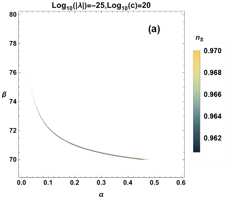
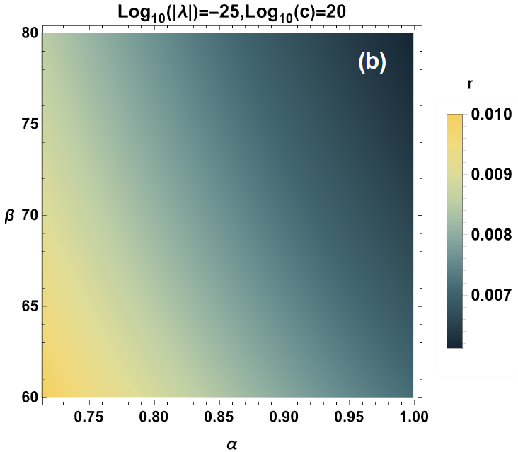
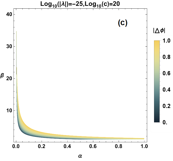
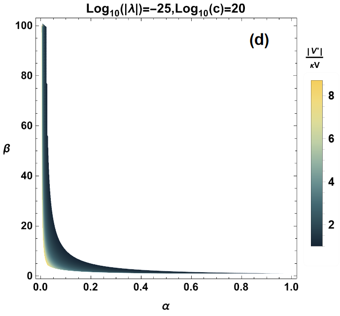
Figure 1: (a): Scalar index $n_{s}$ in terms of the free parameter $\beta$ and scaling parameter $\alpha$. (b): Scalar to tensor ratio $r$ in terms of $\beta$ and $\alpha$. (c): Distance conjecture compatible values $\Delta\phi$ in terms of $\beta$ and $\alpha$. (d): De Sitter conjecture bound runway instability values $\frac{|V^{\prime}|}{\kappa V}$ in terms of $\beta$ and $\alpha$.

It is worth noting that the tachyonic instability values are not approached due to the absence of the de Sitter conjecture bound values in the selected free parameter ranges.

2.  Models with $n\geq 3$

Here, we consider certain specific models with $n\geq 3$. Precisely, we study the models with $n=3$, $n=4$, and $n=5$ by considering different points in the moduli space. Instead of giving graphical discussions, we only provide the numerical values of the involved quantities being summarized in the Table 1.

	$n=3$ for the point	$n=4$ for the point	$n=5$ for the point
	${\scriptscriptstyle(\lambda=-10^{-25},c=10^{20},N=50,\beta=40,\alpha=0.9)}$	${\scriptscriptstyle(\lambda=-10^{-25},c=10^{20},N=50,\beta=50.2,\alpha=0.9)}$	${\scriptscriptstyle(\lambda=-10^{-30},c=10^{20},N=50,\beta=52.7,\alpha=0.9)}$
$n_{S}$	$0.961672127$	$0.966385067$	$0.966511965$
$r$	$0.00888221804$	$0.00762708206$	$0.00686550513$
$n_{\tau}$	$-0.0011027726$	$-0.00953385257$	$-0.00858188141$
$|\Delta\phi|$	$3.17418861$	$2.02584505$	$1.47910070$
$\frac{|V|}{\kappa V}$	$0.0325471498$	$0.0340702087$	$0.0308794845$
$-\frac{V^{\prime\prime}}{\kappa^{2}V}$	$-0.00105931703$	$-0.00116077904$	$-0.00953542476$

Table 1: Numerical values of the models $n=3$, $n=4$ and $n=5$.

Taking in account the numerical approach, we should take the showcased values with a grain of salt, where it has been observed that the value of $\phi_{i}$ being a solution of Eq.(III.4) has been found with an error of the order $\mathcal{O}(10^{-2})$. Nonetheless, the characteristics of the models are not effected by such an error.
For the selected values of $n$, it follows from the table that the scalar spectral index, the scalar to tensor ratio and the tensor spectral index values match perfectly with the observational data. Concerning, the stringy constraint, one can calculate $\delta=|\Delta-\frac{r}{|n_{\tau}|}|$ for different values of $n$. Taking $n=3$, we find $\delta=0$. For $n=4$ and $n=5$, however, we obtain $\delta=2.403\ 10^{-4}$ and $\delta=3.81\ 10^{-6}$, respectively. It is observed that the discrepancy with the stringy constraint grows by increasing $n$. This can be compensated by taking very small values of the coupling constant $\lambda$, rendering a conventional inflationary theory. Such small values do not reflect on the order of the differential forms of the coupling functions. At the chosen moduli space point, for $n=3$, we have found $\xi^{\prime}=-9.22\ 10^{-4}$ and $\xi^{\prime\prime}=-0.144844$. However, the choice of the small value of the coupling constant could insure the consistency with the stringy constraint $r\approx-\Delta n_{\tau}$. This characteristic is a consequence of the non-normalizable coupling function, where the naturalness argument appears to have effect on the relevant quantities.
Moreover, a close inspection shows that the field distance decreases by increasing $n$. For $\mathcal{O}(10)$ order values of $\beta\sqrt{\alpha}$, we obtain $\phi_{f}\approx 1$ and $|\Delta\phi|<1$ satisfying the distance conjecture.

Regarding the de Sitter conjecture, we remark that it is not met for the selected values of $n$. In fact, it has been assumed that all the possible models in this frame do not adhere to the said conjecture. This discrepancy is a characteristic of such an inflationary theory, as pointed in [50]. In an epistemological approach, such an effort concerns the falsification aspects of the theory, where the absence of such an aspect indicates a very large string-landscape/moduli-space of the effective field theory. This issue is mediated in [43], by implementing normalizable coupling functions, since the naturalness of the effective field theory seems to have effects on the relevant quantities.

V.  Conclusion

In this paper, we have investigated the inflationary hypergeometric behaviors in the swampland program via the falsification scenario. In particular, we have exposed the swampland criteria for GB stringy corrections in the rescaled gravity within a linear function of the Ricci scalar namely $F(R)=\alpha R$. Using special functions, we have proposed and examined inflationary models from hypergeometric scalar coupling scenarios. Concretely, we have provided generalized exponential potentials from such hypergeometric behaviors in the swampland program. Precisely, we have considered selected models with different values of the parameter $n$ by means of the slow-roll mechanism. For $n=2$, we have given numerical and graphical investigations by computing the relevant quantities which are found to be compatible with the empirical Planck data. The swampland aspect seems to have the characteristics postulated for conventional inflationary theories. For $n=3$, $n=4$ and $n=5$, however, we summarized the obtained values in Table 1. Analyzing this table, we have observed the compatibility of the Planck observational data. Via a numerical manner, we have shed light on the discussion provided in [50], regarding the discrepancy of the swampland criteria with conventional inflationary models, namely the de Sitter conjecture.

This works comes up with certain open issues. One of them is to consider extra coupling scenarios inspired by string theory corrections which could bring complete differential equations associated with special functions. Other questions could arise including the extant of the naturalness argument effects on the relevant quantities of the effective field theory in connection with swampland program. These questions could be addressed elsewhere.

References

- [1] M. Montero, C. Vafa, I. Valenzuela, The Dark Dimension and the Swampland, J. High Energ. Phys. 02(2023)22.
- [2] J. A. P. Law-Smith, G. Obied, A. Prabhu, C. Vafa, Astrophysical Constraints on Decaying Dark Gravitons, arXiv:2307.11048.
- [3] L. Anchordoqui, I. Antoniadis, D. Lust, The Dark Dimension, the Swampland, and the Dark Matter Fraction Composed of Primordial Black Holes, Phys. Rev. D 10651(2022), arXiv:2206.07071.
- [4] S. Kachru, R. Kallosh, A. Linde, S. P. Trivedi, de Sitter Vacua in String Theory, Phys. Rev. D68 (2003) 046005, hep-th/0301240.
- [5] C. Beasley and E. Witten, A Note on Fluxes and Superpotentials in M-theory Compactifications on Manifolds of Holonomy, JHEP 07 (2002) 046, hep-th/0203061.
- [6] B.S. Acharya, F. Denef and R. Valandro, Statistics of M theory Vacua, JHEP 06 (2005) 056, hep-th/0502060.
- [7] L. Randall, R. Sundrum, A Large Mass Hierarchy from a Small Extra Dimension, Phys. Rev. Lett. 83 (1999) 337, arXiv:hep-ph/9905221.
- [8] L. Randall, R. Sundrum, An Alternative to Compactification, Phys. Rev. Lett. 83 (1999) 4690, arXiv:hep-th/9906064.
- [9] A. Belhaj, M. Benali, Y. Hassouni, M. Oualaid and M. B. Sedra, On brane cosmological behaviors of Starobinsky inflationary model, Int. J. Mod. Phys. A 37 (2022) 2250043.
- [10] A. Belhaj, Y. Hassouni, M. Oualaid and M. B. Sedra, On stringy inflation potentials, Mod. Phys. Lett. A 36(2021) 2150225.
- [11] A. D. Linde, A New Inflationary Universe Scenario: A Possible Solution of the Horizon, Flatness, Homogeneity, Isotropy and Primordial Monopole Problems, Phys. Lett. B108 (1982) 393.
- [12] A. H. Guth, The Inflationary Universe: A Possible Solution to the Horizon and Flatness Problems, Phys. Rev. D23 (1981) 356.
- [13] R. Brandenberger, Topics in Cosmology, PoS P 2GC (2006) 007, arXiv:hep-th/0701157.
- [14] M. Scalisi, Inflation, Higher Spins and the Swampland, Physics Letters B 808 (2020) 135683, arXiv:1912.04283.
- [15] K. Schmitz, Trans-Planckian Censorship and Inflation in Grand Unified Theories, Phys. Lett. B803 (2020)135317, arXiv:1910.08837.
- [16] D. Y. Cheong, S. M. Lee, S. C. Park, Higgs Inflation and the Refined dS Conjecture, Phys. Lett. B789 (2019) 336, arXiv:1811.03622.
- [17] A. Ashoorioon, Rescuing Single Field Inflation from the Swampland, Phys.Lett. B790 (2019) 568, arXiv:1810.04001.
- [18] P. A. R. Ade et al., Planck Collaboration (Planck 2015 results. XX. Constraints on inflation), Astron. and Astrophys 594 (2016) 20, arXiv:1502.02114.
- [19] N. Aghanim et al., Planck Collaboration ( Planck 2018 results.VI. Cosmological parameters), Astron. and Astrophys. 641 (2018) 1432, arXiv:1807.06209.
- [20] Y. Akrami et al. Planck 2018 results. X. Constraints on inflation, Astron. Astrophys. 641 (2020) 10, arXiv:1807.06211.
- [21] P. A. R. Ade et al., Improved Constraints on Primordial Gravitational Waves using Planck, WMAP, and BICEP/Keck Observations through the 2018 Observing Season, Phys. Rev. Lett. 127 (2021) 151301, arXiv:2110.00483.
- [22] S. Koh, B.-H. Lee, W. Lee, and G. Tumurtushaa, Observational constraints on slow-roll inflation coupled to a Gauss-Bonnet term, Phys. Rev. D 90 no. 6, (2014) 063527, arXiv:1404.6096.
- [23] Z. Yi, Y. Gong, and M. Sabir, nflation with Gauss-Bonnet coupling, Phys. Rev. D 98 no. 8, (2018) 083521, arXiv:1804.09116.
- [24] S. D. Odintsov and V. K. Oikonomou, Viable Inflation in Scalar-Gauss-Bonnet Gravity and Reconstruction from Observational Indices, Phys. Rev. D 98 no. 4, (2018) 044039, arXiv:1808.05045.
- [25] S. D. Odintsov and T. Paul, From inflation to reheating and their dynamical stability analysis in Gauss–Bonnet gravity, Phys. Dark Univ. 42 (2023) 101263, arXiv:2305.19110.
- [26] S. Nojiri, S.D. Odintsov, V.K. Oikonomou, Modified Gravity Theories on a Nutshell: Inflation, Bounce and Late-time Evolution, Phys.Rept. 692 (2017) 1, arXiv:1705.11098.
- [27] S.D. Odintsov, V.K. Oikonomou, I. Giannakoudi, F.P. Fronimos, E.C. Lymperiadou, Recent Advances on Inflation, Symmetry 15 (2023) 9, 1701, arXiv:2307.16308.
- [28] D. Iosifidis, R. Myrzakulov, L. Ravera, G. Yergaliyeva, K. Yerzhanov, Metric-Affine Vector-Tensor Correspondence and Implications in F(R,T,Q,T,D) gravity, Phys. Dark Univ. 37 (2022)101094.
- [29] S. Bekov, K. Myrzakulov, R. Myrzakulov, Diego Sáez-Chillón Gómez, General slow-roll inflation in f(R) gravity under the Palatini approach, Symmetry 12 (2020)1958.
- [30] N. Shiníchi and O. D. Sergei, Dark energy, inflation and dark matter from modified F(R) gravity, TSPU Bulletin N8(110) (2011) 7, arXiv:0807.0685.
- [31] V. K. Oikonomou, Unifying inflation with early and late dark energy epochs in axion gravity, Phys. Rev. D103 (2021) 044036, arXiv:2012.00586.
- [32] J. Bora, D. J. Gogoi, U. D. Goswami, Strange stars in f(R) gravity Palatini formalism and gravitational wave echoes from them, JCAP 09 (2022) 057, arXiv:2204.05473.
- [33] A. Belhaj, M. Benali, S.E. Ennadifi, M. Lamaaoune, On inflation scenarios and dark energy in a scaled gravity, Int.J.Geom.Meth.Mod.Phys. 20 (2023) 2350167.
- [34] P. Chaturvedi, U. Kumar, U. Thattarampilly, V. Kakkat, Exact rotating black hole solutions for f(R) gravity by modified Newman Janis algorithm, Eur.Phys.J.C 83 (2023) 1124, arXiv:2309.17044.
- [35] R. Kawaguchi and S. Tsujikawa, Primordial black holes from Higgs inflation with a Gauss-Bonnet coupling, Phys. Rev. D 107 no. 6, (2023) 063508, arXiv:2211.13364.
- [36] V. K. Oikonomou, Unifying inflation with early and late dark energy epochs in axion gravity, Phys. Rev. D 103 (2021) 044036, arXiv:2012.00586.
- [37] B. Li and J. D. Barrow, The Cosmology of f(R) gravity in metric variational approach, Phys. Rev. D 75 (2007) 084010, arXiv:gr-qc/0701111.
- [38] K. Bamba, S. Nojiri, S. D. Odintsov and D. Sáez-Gómez, Inflationary universe from perfect fluid and gravity and its comparison with observational data, Phys. Rev. D 90 (2014) 124061, arXiv:1410.3993.
- [39] V. K. Oikonomou, Singular Bouncing Cosmology from Gauss-Bonnet Modified Gravity, Phys. Rev. D 92 (2015) 124027, arXiv:1509.05827.
- [40] V. K. Oikonomou, A refined Einstein–Gauss–Bonnet inflationary theoretical framework, Class. Quant. Grav. 38 (2021) 195025, arXiv:2108.10460.
- [41] A. Belhaj, M. Benali, Y. Hassouni, M. Lamaaoune, On inflationary models in f(R,T) gravity with a kinetic coupling term, Int.J.Mod.Phys.A 38 (2023) 2350043.
- [42] V. K. Oikonomou, K-R. Revis, I. C. Papadimitriou, M-M. Pegioudi, Swampland Criteria and Constraints on Inflation in a f(R,T) Gravity Theory, Int.J.Mod.Phys.D 32 (2023) 2350034.
- [43] V. K. Oikonomou, I. Giannakoudi, A. Gitsis, K-R. Revis, Rescaled Einstein-Hilbert Gravity: Inflation and the Swampland Criteria, arXiv:2105.11935.
- [44] V. K. Oikonomou, Rescaled Einstein-Hilbert Gravity from f(R) Gravity: Inflation, Dark Energy and the Swampland Criteria, Phys. Rev. D 103, 124028 (2021), arXiv:2012.01312.
- [45] S. D. Odintsov, V. K. Oikonomou, F. P. Fronimos, K. V. Fasoulakos, Unification of a Bounce with a Viable Dark Energy Era in Gauss-Bonnet Gravity, arXiv:2010.13580.
- [46] S. D. Odintsov, V. K. Oikonomou and F. P. Fronimos,Rectifying Einstein-Gauss-Bonnet Inflation in View of GW17081, Nucl. Phys. B 958 (2020)115135, arXiv:2003.13724.
- [47] E.O. Pozdeevaa, M.A. Skugorevab, A.V. Toporensky, S.Yu. Vernova, New slow-roll approximations for inflation in Einstein–Gauss–Bonnet gravity, Phys. Rev. D 103, 124028 (2021), arXiv:2403.06147.
- [48] A. Gitsis, K. R. Revis, S.A. Venikoudis, F.P. Fronimo Swampland criteria for rescaled Einstein- Hilbert gravity with string corrections, arXiv:2301.08126.
- [49] C. Vafa, The String Landscape and the Swampland, arXiv:hep-th/0509212.
- [50] N. B. Agmon, A. Bedroya, M. J. Kang, C. Vafa, Lectures on the string landscape and the Swampland, arXiv:2212.06187.
- [51] E. Palti, C. Vafa, T. Weigand, Supersymmetric Protection and the Swampland, arXiv:2003.10452.
- [52] G. Obied, H. Ooguri, L. Spodyneiko and C. Vafa, De Sitter Space and the Swampland, arXiv:1806.08362.
- [53] D. Lust, E. Palti and C. Vafa, AdS and the Swampland, Phys. Lett. B 797 (2019) 134867, arXiv: 1906.05225.
- [54] H. Ooguri and C. Vafa, On the Geometry of the String Landscape and the Swampland, Nucl. Phys. B 766 (2007) 21, arXiv:hep-th/0605264.
- [55] J. C. Hwang and H. Noh,Classical evolution and quantum generation in generalized gravity theories including string corrections and tachyon: Unified analyses, Phys. Rev. D 71 (2005)063536, arXiv:gr-qc/0412126.
- [56] S. A. Venikoudis and F. P. Fronimos, Inflation with Gauss-Bonnet and Chern-Simons higher-curvature-corrections in the view of GW170817, Gen. Rel. Grav. 53 (2021)75, arXiv:2107.09457.