Influence of fluid rheology on multistability in the unstable flow of polymer solutions through pore constriction arrays

Abstract

Diverse chemical, energy, environmental, and industrial processes involve the flow of polymer solutions in porous media. The accumulation and dissipation of elastic stresses as the polymers are transported through the tortuous, confined pore space can lead to the development of an elastic flow instability above a threshold flow rate. This flow instability can generate complex flows with strong spatiotemporal fluctuations, despite the low Reynolds number ($\mathrm{Re}\ll 1$); for example, in 1D ordered arrays of pore constrictions, this unstable flow can be multistable, with distinct pores exhibiting distinct unstable flow states. Here, we examine how this multistability is influenced by fluid rheology. Through experiments using diverse polymer solutions having systematic variations in fluid shear-thinning or elasticity, in pore constriction arrays of varying geometries, we show that the onset of multistability can be described using a single dimensionless parameter. This parameter, the streamwise Deborah number, compares the stress relaxation time of the polymer solution to the time required for the fluid to be advected between pore constrictions. Our work thus helps to deepen understanding of the influence of fluid rheology on elastic instabilities, helping to establish guidelines for the rational design of polymeric fluids with desirable flow behaviors.

I Introduction

A wide range of energy, environmental, industrial, and laboratory processes rely on the slow flow of solutions of large flexible polymers through porous media; examples include separations Kozicki and Slegr (1994); Luo and Teraoka (1996); Bourgeat, Gipouloux, and Marusic-Paloka (2003), chemical production Petrie and Denn (1976); Denn (2008); Turner, Strong, and Gold (2014); Elbadawi (2018), enhanced oil recovery Durst, Haas, and Kaczmar (1981); Seright et al. (2010); Sorbie (2013); Clarke et al. (2016); Pogaku et al. (2018); Mirzaie Yegane, Boukany, and Zitha (2022), groundwater remediation Roote (1998); Smith et al. (2008); Huo et al. (2020); Hartmann et al. (2021), and geothermal energy production Di Dato et al. (2022). These processes require the spatiotemporal characteristics of the pore-scale flow to be predictable and controllable. However, the flow behavior typically depends on a complex interplay between the solution properties, imposed flow conditions, and porous medium geometry—all of which can vary greatly in practice—that is still poorly understood. Consequently, such processes often proceed by trial and error. Here, we take a step towards addressing this gap in knowledge by systematically studying how variations in polymer solution rheology influence flow in model porous media with precisely-defined geometries.

Such polymer solutions have two key rheological characteristics. First, they are often shear-thinning: the dynamic shear viscosity $\eta$ of a given solution decreases with increasing shear rate $\dot{\gamma}$, reflecting stretching and alignment of the constituent polymer chains under flow Macosko (1994); Larson (1999); Rubinstein and Colby (2003); Ryder and Yeomans (2006). Second, they are often highly elastic: the first normal stress difference $N_{1}$ of the solution is non-negligible and increases with shear rate in e.g., a cone-plate rheometer, reflecting the normal elastic stresses that arise as the polymer chains are stretched along the curved fluid streamlines Larson (1992); McKinley, Pakdel, and Öztekin (1996); Pakdel and McKinley (1996). These elastic stresses can have dramatic consequences. A familiar example is the Weissenberg effect, in which the polymer solution “climbs” up a spinning rod inserted into it instead of being ejected away by inertia Weissenberg (1947); Bird, Armstrong, and Hassager (1987); More et al. (2023). At sufficiently large flow speeds, these stresses accumulate faster than they can relax, causing the flow to become unstable—as exemplified in studies across a wide array of model geometries that feature curved streamlines Datta et al. (2022). These studies have shown that such purely-elastic instabilities — termed such because they arise due to fluid elasticity, not inertia, at low Reynolds number $\textrm{Re}\ll 1$ Pearson (1976); Larson (1992); Pakdel and McKinley (1996); Shaqfeh (1996) — can generate secondary flows McKinley, Pakdel, and Öztekin (1996); Pakdel and McKinley (1996); Groisman and Steinberg (2001); Ducloué et al. (2019); Shakeri, Jung, and Seemann (2022a), eddies and vortices Batchelor (1971); Boger (1987); Koelling and Prud’homme (1991); Byars et al. (1994); Mongruel and Cloitre (1995); Khomami and Moreno (1997); Arora, Sureshkumar, and Khomami (2002); Mongruel and Cloitre (2003); Groisman and Steinberg (2000); Rodd et al. (2007); Lanzaro and Yuan (2011); Kenney et al. (2013); Gulati, Muller, and Liepmann (2015); Shi and Christopher (2016); Varshney and Steinberg (2017); Qin et al. (2019); Hopkins, Haward, and Shen (2022), periodic flow fluctuations Sousa, Pinho, and Alves (2018); Hopkins, Haward, and Shen (2020), dead zones Kawale et al. (2017a, b); Kawale, Jayaraman, and Boukany (2019); Ichikawa and Motosuke (2022), flow asymmetries Arratia et al. (2006); Galindo-Rosales, Oliveira, and Alves (2014); Ribeiro et al. (2014); Haward, McKinley, and Shen (2016); Lanzaro, Corbett, and Yuan (2017); Haward, Toda-Peters, and Shen (2018); Davoodi, Domingues, and Poole (2019); Qin et al. (2020); Yokokoji et al. (2023); Kumar et al. (2023), and even chaotic flows with a broad spectrum of spatial and temporal fluctuations Groisman and Steinberg (1998, 2000, 2001); Pan et al. (2013); Scholz et al. (2014); Clarke et al. (2015); Howe, Clarke, and Giernalczyk (2015); Lanzaro, Li, and Yuan (2015); Traore, Castelain, and Burghelea (2015); Whalley et al. (2015); Clarke et al. (2016); Mitchell et al. (2016); Qin and Arratia (2017); Browne and Datta (2021); Shakeri, Jung, and Seemann (2021); Carlson et al. (2022); Browne et al. (2023); Browne and Datta (2023), depending on the properties of the confining boundaries and imposed flow conditions.

To isolate the influence of fluid elasticity from shear-thinning, elastic instabilities are commonly studied using Boger fluids Boger (1987); James (2009) — elastic but non-shear-thinning fluids composed of dilute amounts of the polymer dispersed in a highly-viscous solvent. However, the polymer solutions used in energy, environmental, industrial, and laboratory processes often differ from this idealized limit, exhibiting varying degrees of shear-thinning and elasticity Howe, Clarke, and Giernalczyk (2015); Clarke et al. (2016); Mirzaie Yegane, Boukany, and Zitha (2022). Studies in simplified geometries indicate that such variations in solution rheology can strongly influence how elastic instabilities manifest Larson, Muller, and Shaqfeh (1994); McKinley, Pakdel, and Öztekin (1996); Jagdale et al. (2020); Yokokoji et al. (2023), with some studies even suggesting that shear-thinning suppresses the onset of elastic instabilities altogether Larson, Muller, and Shaqfeh (1994); Casanellas et al. (2016); Cagney, Lacassagne, and Balabani (2020); Lacassagne, Cagney, and Balabani (2021). However, decoupling the influence of shear-thinning and fluid elasticity is challenging in more geometrically-complex porous media in which the pore space geometry and thus, local flow conditions, are spatially highly heterogeneous.

In previous work Browne, Shih, and Datta (2020a), we used microfabricated one-dimensional (1D) ordered arrays of pore constrictions [schematized in Figure 1(a)] to simplify this complexity. By directly visualizing the flow of an approximately Boger fluid through these arrays, we found that when the spacing between adjacent constrictions is sufficiently small, the unstable flow exhibits multistability: it stochastically switches between distinct unstable flow states in the distinct pores. In the “eddy-dominated” state, large unstable eddies form in the corners of a given pore body in between adjacent constrictions; by contrast, in the “eddy-free” state, strongly fluctuating fluid pathlines fill the entire pore body and eddies do not form. Theoretical calculations, supported by the simulations of Kumar et al., indicated that this unusual behavior arises from the competition between flow-induced polymer elongation, which promotes eddy formation Batchelor (1971); Boger (1987); Mongruel and Cloitre (1995, 2003); Rodd et al. (2007), and relaxation of polymers as they are advected between pore constrictions, causing elastic stresses to dissipate and enabling the eddy-free state to form. However, as in typical studies of elastic flow instabilities, this study used an elastic fluid that does not exhibit appreciable shear-thinning—despite the prevalence and importance of shear-thinning fluids in many real-world settings. Hence, we ask: How does shear-thinning influence the onset and features of this multistability?

Here, we address this question by experimentally studying the flow of polymer solutions with distinct rheological characteristics through 1D ordered arrays of pore constrictions. The solutions have systematic variations in either their degree of shear-thinning or fluid elasticity, enabling us to decouple the influence of these two rheological characteristics. Consistent with our prior work, we find that the fluid must be sufficiently elastic to become unstable and exhibit multistability. Moreover, we find that shear-thinning does not abrogate the onset of the elastic instability and the resulting development of multistability; however, it does influence the conditions at which multistability arises. In particular, for all polymer solutions tested, multistability arises when a characteristic stress relaxation time of the solution $\lambda$ approximately exceeds the characteristic time $t_{\mathrm{adv}}$ for fluid to be advected between pore constrictions; for non-shear-thinning solutions, $\lambda$ is given by the shear rate-independent longest stress relaxation time of the solution, whereas for shear-thinning solutions, $\lambda$ is instead rate-dependent. These results thus help expand understanding of flow multistability in porous media to a broader class of fluids, providing a way to use bulk rheology measurements to predict and control the pore-scale dynamics of unstable polymer solution flows. Not only does our work thereby deepen understanding of elastic instabilities, but it highlights a potentially useful way to harness such instabilities to alter momentum and mass transport in porous media Groisman and Steinberg (2001); Burghelea et al. (2004); Pathak, Ross, and Migler (2004); Scholz et al. (2014); Traore, Castelain, and Burghelea (2015); Whalley et al. (2015); Kumar et al. (2023); Browne and Datta (2023).

II Materials and Methods

II.1 Device fabrication

We follow our previous work Browne, Shih, and Datta (2020a) in designing and fabricating the millifluidic devices used in the experiments. As shown in Fig. 1(a), each device has a straight square channel $W_{0}=2$ mm wide and $H=2$ mm high with pore constrictions, evenly spaced by a distance $l_{s}$, defined by opposing hemi-cylindrical posts of diameter $D_{p}=1.6$ mm. To vary the extent to which elastic stresses can be retained between pore constrictions before relaxing, we test three different constriction-to-constriction spacings: $l_{s}=1W_{0}$, $1.3W_{0}$, and $1.6W_{0}$. The devices have either 30 ($l_{s}=W_{0}$) or 20 ($l_{s}=1.3W_{0}$ and $1.6W_{0}$) pore constrictions in total. For each device, we define the characteristic volume of a pore body as $V_{\mathrm{pore}}=HA_{\mathrm{pore}}$, where $A_{\mathrm{pore}}=l_{s}W_{0}-\pi D_{p}^{2}/4$.

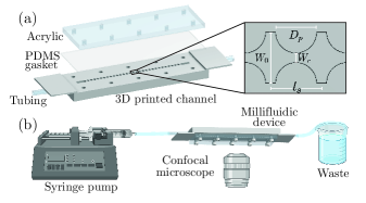
Figure 1: Schematic of the millifluidic device and experimental approach. (a) We fabricate millifluidic devices composed of a 3D-printed channel sealed by an overlying PDMS gasket and transparent acrylic top sheet, which allows for direct imaging of the flow within the channel. The inset shows the channel geometry: the square channel has width $W_{0}$ and height $H$, and pore constrictions of width $W_{c}$ are defined by opposing hemi-cylindrical posts of diameter $D_{p}$ spaced by a streamwise length $l_{s}$. (b) Each device is mounted on the stage of a confocal microscope used to directly image fluorescent tracers in the fluid, injected at a constant volumetric flow rate using a syringe pump. Figure created with biorender.com.

We design each device using CAD software (Onshape) and 3D-print it using a proprietary clear polymeric resin made of methacrylate oligomers and photoinitiators (FLGPCL04) cured in a FormLabs Form 3 stereolithography 3D printer. Overlying the 3D-printed channel is a laser-cut clear acrylic top sheet fitted with screwholes (Epilog Mini 24). We sandwich a $\sim 1$ mm thick sheet of polydimethylsiloxane (PDMS; Dow SYLGARD 184), made using a base-to-curing agent ratio of 8.5:1.5 by weight, between the 3D-printed channel and laser-cut acrylic top sheet to act as a gasket and ensure a watertight seal; each device is assembled by tightly screwing together the channel, PDMS, and acrylic layers. Finally, we glue flexible Tygon tubing (McMaster-Carr) into the inlets and outlets using a watertight two-part epoxy (JB MarineWeld).

II.2 Fluid formulations

We test eight different fluids, carefully formulated to have systematic variations in their degree of shear-thinning or fluid elasticity:

• Pure glycerol (Acros Organics)—a Newtonian, non-shear-thinning, non-elastic fluid that acts as a negative control.

• 900 ppm xanthan gum (Sigma-Aldrich) dissolved in ultrapure (Milli-Q) water—a highly shear-thinning but not appreciably elastic fluid. This formulation is an entangled Dobrynin, Colby, and Rubinstein (1995); Howe, Clarke, and Giernalczyk (2015); Tran and Clarke (2023) semi-dilute polymer solution ($c/c^{*}\approx 13$ Wyatt and Liberatore (2009)), where $c^{*}$ is the overlap concentration at which adjacent polymer chains begin to interact with each other under quiescent conditions Rubinstein and Colby (2003).

• 300 ppm 30% hydrolyzed $18$ MDa polyacrylamide (HPAM; Polysciences) dissolved in 89% glycerol, 10% ultrapure water, and 1% NaCl (Sigma-Aldrich)—a not appreciably shear-thinning but highly elastic fluid. This formulation is a dilute polymer solution ($c/c^{*}\approx 0.33$ Browne, Shih, and Datta (2020a)).

• 300 ppm HPAM dissolved in 82.6% glycerol, 10.4% dimethyl sulfoxide (DMSO; Sigma-Aldrich), 6% ultrapure water, and 1% NaCl—another not appreciably shear-thinning but highly elastic fluid. This formulation is a dilute polymer solution ($c/c^{*}\approx 0.5$ Browne and Datta (2021)).

• 900 ppm HPAM dissolved in the same glycerol-DMSO-water-NaCl solvent—a moderately shear-thinning and highly elastic fluid. This formulation is an unentangled semi-dilute polymer solution ($c/c^{*}\approx 1.5$ Browne and Datta (2021)).

• 4500 ppm HPAM dissolved in 89% glycerol, 10% ultrapure water, and 1% NaCl—a highly shear-thinning and highly elastic fluid. This formulation is an unentangled semi-dilute polymer solution ($c/c^{*}\approx 5$ Browne, Shih, and Datta (2020a)).

• 1000 ppm HPAM dissolved in ultrapure water with 1% NaCl—a moderately shear-thinning and moderately elastic fluid. This formulation is an unentangled semi-dilute polymer solution ($c/c^{*}\approx 5$ Liu, Jun, and Steinberg (2009)).

• 3700 ppm HPAM dissolved in ultrapure water with 1% NaCl—a highly shear-thinning and moderately elastic fluid. This formulation is an entangled semi-dilute entangled polymer solution ($c/c^{*}\approx 19$ Liu, Jun, and Steinberg (2009)).

The HPAM solutions have sufficient NaCl such that the ionic strength ($173$ mM) exceeds the charge concentration associated with the HPAM carboxylate groups for all concentrations tested; thus, the HPAM behaves as a flexible, neutral polymer due to excess salt screening in the formulations with NaCl Dobrynin, Colby, and Rubinstein (1995); Howe, Clarke, and Giernalczyk (2015). As a shorthand, hereafter, we refer to aqueous solutions as Aq, glycerol-water solutions as Gl-Aq, and glycerol-water-DMSO solutions as Gl-Aq-DMSO.

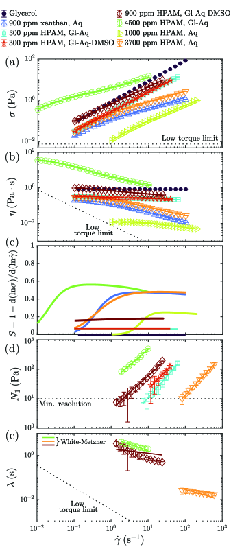
Figure 2: Shear rheology of test solutions. (a) Shear stress $\sigma$ required to maintain an imposed shear rate $\dot{\gamma}$. Error bars show the standard deviation of 3 separate replicates of each solution. (b) Corresponding shear viscosity $\eta=\sigma/\dot{\gamma}$. Solid curves show Carreau-Yasuda or power-law fits, as described in the main text. (c) Corresponding shear-thinning parameter, $S$. (d) First normal stress difference, $N_{1}$. Solid curves show power-law fits. (e) Shear rate-dependent relaxation time, $\lambda(\dot{\gamma})$, determined as described in the main text. The sensitivity of the rheometer limits the resolution in measuring $N_{1}$, and correspondingly in determining $\lambda$ over all $\dot{\gamma}$ tested. Data for solutions with lower values of $N_{1}$ are not shown. Solid curves show White-Metzner fits.

To mix each polymer solution, we first dissolve the polymer in milliQ water in a conical tube on a rotor mixer for one day. We then dilute the solution with the remaining solvent components (glycerol, DMSO, and/or salt), and gently mix for at least 24 hours with a stir bar at 60 rpm to avoid mechanical degradation of the polymer. All polymer solutions are used within one month of mixing to avoid polymer degradation. We also seed each test fluid with 30 ppm of 1 $\upmu$m-diameter, carboxylate-modified polystyrene fluorescent tracer particles (Invitrogen) for flow visualization, as detailed further in §II.4.

Table 1: Rheological parameters for the different test solutions, obtained using bulk shear rheology. Symbols are all defined in the main text. We estimate the zero-shear viscosity using the viscosity at the lowest measured shear rate, $\eta_{0}\approx\eta|_{\dot{\gamma}=0.1\>\mathrm{s^{-1}}}$ for the power law fluids. We set $\eta_{\infty}=\eta_{s}$, the Newtonian solvent viscosity, for fitting as our measurements do not extend to sufficiently high rates to obtain a plateau. For the relaxation time, we use $\dot{\gamma}=1\>\mathrm{s^{-1}}$ as the lowest accessible shear rate within measurement limits to avoid noise from the instrument resolution at lower shear rates.

Solution	$c/c^{*}$	$\eta_{0}$ (Pa$\cdot$s)	$\eta_{\infty}$ (Pa$\cdot$s)	$K_{\sigma}$ $(\mathrm{Pa\cdot s^{\emph{n}}})$	$n$	$\dot{\gamma}_{c}$ $(\mathrm{s^{-1}})$	$a$	$\beta$	$\lambda_{0}$ (s)	$K_{N_{1}}$ $(\mathrm{Pa\cdot s^{\emph{n}_{\emph{N}_{1}}}})$	$n_{N_{1}}$	$\lambda_{0,\mathrm{WM}}$ (s)	$N_{1}|_{10\>\mathrm{s^{-1}}}$ (Pa)	$S_{\mathrm{max}}$
Glycerol	$---$	$0.862$	$---$	$---$	$---$	$---$	$---$	$---$	$---$	$---$	$---$	$---$	$0$	$0$
900 ppm xanthan Aq	$13$	$0.196$	$0.001$	$---$	$0.51$	$0.38$	$2$	$0.005$	$---$	$---$	$---$	$---$	$0$	$0.47$
300 ppm HPAM Gl-Aq	$0.3$	$0.334$	$---$	$0.28$	$0.94$	$---$	$---$	$0.66$	$2.1$	$0.41$	$1.4$	$---$	$10.3$	$0.06$
300 ppm HPAM Gl-Aq-DMSO	$0.5$	$0.33$	$---$	$0.29$	$0.94$	$---$	$---$	$0.19$	$2.2$	$1.3$	$1.2$	$---$	$20.6$	$0.06$
900 ppm HPAM Gl-Aq-DMSO	$1.5$	$5.02$	$0.062$	$---$	$0.73$	$0.006$	$0.15$	$0.01$	$10.6$	$4.3$	$1.1$	$16.3$	$54.1$	$0.18$
4500 ppm HPAM Gl-Aq	$5$	$38.8$	$0.22$	$---$	$0.42$	$0.02$	$1.8$	$0.006$	$28$	$40.5$	$1.1$	$61.5$	$510$	$0.56$
1000 ppm HPAM Aq	$5$	$0.01$	$0.001$	$---$	$0.71$	$6.1$	$2.8$	$0.09$	$0.2$	$---$	$---$	$---$	$---$	$0.25$
3700 ppm HPAM Aq	$18.5$	$0.396$	$0.001$	$---$	$0.51$	$0.4$	$1.3$	$0.003$	$2.0$	$0.03$	$1.3$	$0.44$	$0.60$	$0.48$

II.3 Bulk shear rheology

We characterize the shear rheology of each bulk solution using a stress-controlled Anton Paar MCR501 rheometer fitted with a truncated cone-plate geometry (CP50-2: $50$ mm diameter, $2^{\circ}$, $53~{}\upmu$m gap) and temperature-controlled at $25^{\circ}$C. In particular, we measure steady-state flow curves by ramping up, then ramping down, the imposed shear rate across the range $\dot{\gamma}=0.01-100\>\mathrm{s^{-1}}$ and measure the shear stress $\sigma$ and first normal stress difference $N_{1}$. We do not observe substantial hysteresis with ramping direction in our measurements. The manufacturer-specified minimum torque is $T_{\mathrm{min}}=0.05\>\upmu$N$\cdot$m; we use $5\times$ this quoted minimum value to report the lower limit of resolvable stresses, viscosity, and relaxation time in our measurements. The lower limit of the measured $N_{1}$ is $\sim 10$ Pa due to the normal force sensitivity. For the dilute polymer concentrations, we use a lower shear rate limit of $\dot{\gamma}=0.1\>\mathrm{s^{-1}}$ due to the minimum torque limitations. For solutions with large normal stresses, we only measure up to $\dot{\gamma}\approx 30\>\mathrm{s^{-1}}$ to avoid elastic instabilities that develop in the cone-plate geometry.

Our measurements are summarized in Fig. 2 and Table 1. We first examine the shear-thinning nature of the different fluids. As classified in §II.2, the two 300 ppm HPAM solutions are not appreciably shear-thinning; as shown by the solid lines in Fig. 2(a–b), the shear stress and viscosity vary as $\sigma(\dot{\gamma})=K_{\sigma}\dot{\gamma}^{n}$ and $\eta(\dot{\gamma})=K_{\sigma}\dot{\gamma}^{n-1}$, respectively, where $K_{\sigma}$ is known as the flow consistency index and the power law index $n=0.94\approx 1$, indicating minimal shear-thinning. By contrast, the other polymer solutions show appreciable shear-thinning; as shown by the corresponding solid lines in Fig. 2(a–b), the data are fit well by the Carreau-Yasuda model, $(\eta-\eta_{0})/(\eta_{\infty}-\eta_{0})=(1+(\dot{\gamma}/\dot{\gamma}_{c})^{a})^{(n-1)/a}$, where $\eta_{0}$ is the zero-shear viscosity, $\eta_{\infty}$ is the infinite-shear viscosity, $\dot{\gamma}_{c}$ is the critical shear rate for the onset of shear-thinning, and $a$ is a parameter that controls the transition to the shear-thinning regime. We further characterize this behavior in Fig. 2(c) using the shear-thinning parameter $S\equiv 1-\frac{\mathrm{d(ln}\sigma\mathrm{)}}{\mathrm{d(ln}\dot{\gamma}\mathrm{)}}$, which is 1 minus the slope of the shear stress flow-curve on a log-log plot Haward, Hopkins, and Shen (2020); Yokokoji et al. (2023). For a non-shear-thinning fluid, the maximal measured $S_{\mathrm{max}}\approx 0$, while $0<S_{\mathrm{max}}<1$ for a shear-thinning fluid. As shown in Fig. 3 and classified in §II.2, our solutions are either non-shear-thinning with $S_{\mathrm{max}}\approx 0-0.05$ (glycerol, both 300 ppm HPAM solutions), moderately shear-thinning with $S_{\mathrm{max}}\approx 0.2-0.25$ (1000 ppm HPAM Aq and 900 ppm HPAM Gl-Aq-DMSO), or highly shear-thinning with $S_{\mathrm{max}}\approx 0.5$ (xanthan, 3700 ppm HPAM Aq, and 4500 ppm HPAM Gl-Aq).

Next, we examine the elasticity of the different fluids. Fig. 2(d) shows the measured first normal stress difference with the solid lines indicating power law fits, $N_{1}(\dot{\gamma})=K_{N_{1}}\dot{\gamma}^{n_{N_{1}}}$, where $K_{N_{1}}$ is known as the consistency index and $n_{N_{1}}$ is the power law index for $N_{1}$. We use the value of $N_{1}$ measured at $\dot{\gamma}=10~{}\mathrm{s}^{-1}$, $N_{1}|_{10~{}\mathrm{s}^{-1}}$, as a simple way to characterize the extent of fluid elasticity. As shown in Fig. 3 and classified in §II.2, glycerol and the xanthan solution are non-elastic with a non-measurable $N_{1}|_{10~{}\mathrm{s}^{-1}}\sim 0$, while the 3700 ppm HPAM Aq solution is moderately elastic with $N_{1}|_{10~{}\mathrm{s}^{-1}}\sim 1$ Pa, and the Gl-Aq and Gl-Aq-DMSO HPAM solutions are highly elastic with $N_{1}|_{10~{}\mathrm{s}^{-1}}\approx 10-500$ Pa. The 1000 ppm HPAM Aq solution is also moderately elastic with $N_{1}|_{10~{}\mathrm{s}^{-1}}\lesssim 1$ Pa; however, for this solution, the measured normal stress values are at the noise threshold of the rheometer, and we therefore omit them from Figs. 2–3 given the large measurement uncertainty.

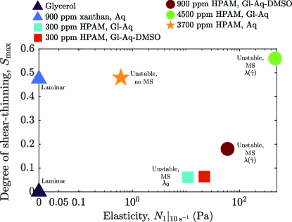
Figure 3: Summary of different test fluids used, with systematically varying degrees of shear-thinning, quantified by the maximal measured shear-thinning parameter $S_{\mathrm{max}}$ from shear rheology, and elasticity, as quantified by the first normal stress difference measured at $\dot{\gamma}=10~{}\mathrm{s}^{-1}$, $N_{1}|_{10~{}\mathrm{s}^{-1}}$. ‘MS’ refers to fluids that exhibit multistability in the experiments.

We use shear stress relaxation measurements to characterize the longest relaxation time of the polymer solutions Liu, Jun, and Steinberg (2007, 2009). In the cone-plate geometry, we impose a constant shear rate $\dot{\gamma}=1\>\mathrm{s^{-1}}$ operating in stress-controlled mode for $60$ s, stop shearing, and record the instantaneous shear stress response as it decays over time $t$. Fitting a single exponential decay as predicted by Maxwell relaxation model, $\sigma(t)\sim e^{-t/\lambda_{0}}$, to the linear portion of the stress-time curve in log-linear coordinates then yields an approximation to the longest relaxation time $\lambda_{0}$, whose values are given in Table 1. This parameter describes the stress relaxation dynamics of non-shear-thinning dilute polymer solutions Boger (1987); James (2009); however, for more concentrated solutions that exhibit shear-thinning, rheological properties exhibit strongly shear rate-dependent behavior Bird, Armstrong, and Hassager (1987); Casanellas et al. (2016); Shakeri, Jung, and Seemann (2022b). To characterize this rate dependence, we determine the relaxation time from the steady-state flow curves as $\lambda(\dot{\gamma})=\frac{N_{1}(\dot{\gamma})}{2\sigma(\dot{\gamma})\dot{\gamma}}\frac{\eta(\dot{\gamma})}{\eta(\dot{\gamma})-\eta_{s}}$ White and Metzner (1963); Bird, Armstrong, and Hassager (1987); Macosko (1994); Casanellas et al. (2016); Qin et al. (2019); here, $\eta_{s}$ is the solvent viscosity, and we thereby define the parameter $\beta\equiv\eta_{s}/\eta_{0}$ to quantify the solvent contribution to the total solution viscosity. The corresponding data are shown in Fig. 2(e). As shown by the solid curves, the data are described reasonably well by the White-Metzner model White and Metzner (1963), $\lambda_{\mathrm{WM}}(\dot{\gamma})=\frac{\lambda_{0,\mathrm{WM}}}{(1+(\dot{\gamma}/\dot{\gamma}_{c})^{a})^{(1-n)/a}}$, where the parameters $\dot{\gamma}_{c}$, $a$, and $n$ are determined from the Carreau-Yasuda fits in Fig. 2(b) and the characteristic relaxation time $\lambda_{0,\mathrm{WM}}$ is a fitting parameter.

II.4 Flow visualization

Prior to each flow experiment, we first flush the millifluidic device to be used with ultrapure (Milli-Q) water, ensuring that no air bubbles are retained in the channel. We then fill the device with pure glycerol, followed by the fluid to be tested at a constant low flow rate of $1.5\>\mathrm{mL/hr}$ using a Harvard Apparatus PHD 2000 syringe pump for at least 3 hours to saturate the pore space. We then mount the millifluidic device on the stage of a Nikon A1R+ laser scanning confocal fluorescence microscope, positioning the set-up so that the syringe pump, device, and outlet waste jar are at the same height to avoid hydrostatic pressure differences [Fig. 1(b)].

During each experiment, we progressively increase the inlet flow rate $Q$ from $0.5$ to $25$ mL/hr, injecting the test fluid for at least 90 min ($>85V_{\mathrm{pore}}$) at each flow rate before commencing imaging to ensure that the flow has reached a near-steady state. We report the results for each flow rate in terms of the shear rate at the constriction wall, $\dot{\gamma}_{w,c}$, defined in §II.5 below. For each flow rate tested, we directly visualize the flow field in the millifluidic device using the confocal microscope, exciting the tracer particles seeded in the test fluid with a 488 nm laser and detecting their fluorescence emission using a 500-550 nm sensor. In particular, we use a $4\times$ objective lens to interrogate a two-dimensional $1583~{}\upmu\text{m}\times 3167~{}\upmu\text{m}$ field of view at a pixel resolution of $\approx 6~{}\upmu\text{m}$ and optical section thickness of $37~{}\upmu\text{m}$ at a fixed depth midway along the height of the channel. We acquire successive such images at a speed of 60 frames per second for two minutes per pore ($\geq 5V_{\mathrm{pore}}$). These sequences of images generate the streakline videos shown in Supplementary Movies 1–2, for which we additionally time-average the intensity in each pixel over a running duration of 30 successive frames to produce streaklines of the tracer particles. Furthermore, to represent the dynamic flow field in the static streakline images provided in the manuscript, we time-average the intensity in each pixel across successive images obtained over a total duration corresponding to $5V_{\mathrm{pore}}$. We use the streakline images to manually measure the combined sizes of any eddies that may arise in the upper and lower corners of a given pore body upstream of a constriction, $A_{\mathrm{eddy}}$.

II.5 Characteristic parameters describing flow

Given that the rheology of the test fluids is shear rate-dependent (Fig. 2), we calculate the characteristic shear rates experienced by the fluids as they are transported through the millifluidic devices. The device channel width varies with streamwise position, $x$, as:

$$W(x)=\begin{cases}W_{0}-2\sqrt{(D_{p}/2)^{2}-(x-D_{p}/2)^{2}}&\text{for $0\leq x<D_{p}$}\\ W_{0}&\text{for $D_{p}\leq x\leq l_{s}.$}\\ \end{cases}$$

The fluid interstitial velocity is then given by $U(x)=Q/HW(x)$, and we thereby define a position-dependent shear rate using the half-width of the channel as the characteristic length scale: $\dot{\gamma}(x)=2U(x)/W(x)=2Q/HW(x)^{2}$. The average shear rate in a pore is then given by $\langle\dot{\gamma}\rangle_{x}=\frac{1}{l_{s}}\int_{0}^{l_{s}}\dot{\gamma}(x)\mathrm{d}x.$ We also calculate the shear rate at the channel wall, $\dot{\gamma}_{w}(x)=\left(\frac{6Q}{WH^{2}}\right)\left(1+\frac{H}{W}\right)\left(\frac{2}{3}f^{*}\right)\left(\frac{b^{*}}{f^{*}}+\frac{a^{*}}{f^{*}}\frac{1}{n}\right)$, following Harnett and  Son; here, $a^{*}$, $b^{*}$, and $f^{*}$ are constants determined from numerical calculations that depend on the channel aspect ratio Harnett (1989). The wall shear rate takes on its maximal value, $\dot{\gamma}_{w,c}=\dot{\gamma}_{w}(W_{c})$, at the pore constrictions with $a^{*}=0.3475,\ b^{*}=0.8444$, $f^{*}=0.7946$, and $H/W_{c}=5$.

The flow can then be described by four dimensionless parameters:

• The Reynolds number comparing the strength of inertial to viscous stresses, $\mathrm{Re}=\rho U_{c}W_{c}/\eta_{0}$. Here, $\rho$ is the fluid density, $U_{c}=Q/HW_{c}$ is the average velocity in a pore constriction, and $W_{c}=0.4$ mm is the channel width at the constriction. Across all fluids and flow conditions tested, $\mathrm{Re}\lesssim 10^{-1}$, indicating that inertial effects are negligible.

• The Weissenberg number comparing the strength of elastic to viscous stresses, $\mathrm{Wi}=\frac{N_{1}(\dot{\gamma}_{w,c})}{2\sigma(\dot{\gamma}_{w,c})}$. Our experiments are characterized by $\mathrm{Wi}=0$ to $67$, indicating that elastic stresses can become sufficiently large to generate purely-elastic instabilities during flow.

• The Pakdel-McKinley number describing the loss of flow stability when sufficiently large elastic stresses propagate over sufficiently long timescales along curved streamlines McKinley, Pakdel, and Öztekin (1996); Pakdel and McKinley (1996), $\mathrm{M}=\sqrt{2\mathrm{Wi}\cdot\mathrm{De}_{\mathcal{R}}}$. Here, $\mathrm{De}_{\mathcal{R}}=\lambda/\left(\mathcal{R}/U_{c}\right)$, where $\mathcal{R}\approx(2/D_{p}+32.5/W_{0})^{-1}$ is the characteristic streamline radius of curvature McKinley, Pakdel, and Öztekin (1996). Our experiments are characterized by $\mathrm{M}=0$ to $316$, indicating again that elastic stresses can become sufficiently large and persistent over time to generate purely-elastic instabilities during flow.

• The streamwise Deborah number comparing the fluid relaxation time to the characteristic time $t_{\mathrm{adv}}$ for fluid to be advected between pore constrictions, $\mathrm{De}=\lambda/t_{\mathrm{adv}}$. Here, $\lambda=\lambda_{0}$ or $\lambda_{\mathrm{WM}}(\dot{\gamma})$ for non-shear-thinning or shear-thinning fluids, respectively, and $t_{\mathrm{adv}}=V_{c}/Q$, where we define the characteristic volume of the straight channel extending between pores that is circumscribed by the cylindrical posts, $V_{c}=l_{s}W_{c}H$. As described further in §III.3, the central result of this paper is that $\mathrm{De}$ describes the onset of multistability across all fluids tested in this work.

III Results and Discussion

III.1 Multistability of a highly-elastic, non-shear-thinning fluid

We first examine the flow of a highly-elastic, but non-shear-thinning, fluid (300 ppm HPAM, Gl-Aq—light blue square in Fig. 3) in a device with $l_{s}=W_{0}$. Streakline images of the flow in two neighboring pores near the middle of the device are shown in Figs. 4(a–b). As exemplified by the leftmost panels, at low flow rates, the flow is laminar throughout the entire pore space; it remains steady over time, with small Moffatt eddies in the corners upstream of each constriction. Above a threshold flow rate, however, the flow becomes unstable: the flow velocities fluctuate both spatially and temporally. An example is shown by the crossing streaklines in the righthand panels of Figs. 4(a–b), which represent the flow at three different times. We quantify the onset of this elastic instability by measuring the root-mean-square temporal fluctuations in the size $A_{\mathrm{eddy}}$ of each eddy, $A^{\prime}_{\mathrm{eddy,rms}}$, where the prime indicates fluctuations from the mean value, $\langle A_{\mathrm{eddy}}\rangle_{t}$. The open square symbols in Fig. 4(e) show these measurements aggregated across multiple pore bodies of the medium. Consistent with the flow images shown in Figs. 4(a–b), $\mathcal{A}\equiv A^{\prime}_{\mathrm{eddy,rms}}/\langle A_{\mathrm{eddy}}\rangle_{t}$ increases above the noise threshold at a constriction wall shear rate $\dot{\gamma}_{w,c}\sim 4-10\>\mathrm{s^{-1}}$, corresponding to $\mathrm{Wi}\sim 2-6$ and $\mathrm{M}\sim 6-19$. By contrast, Newtonian glycerol or a shear-thinning but non-elastic xanthan solution remain laminar at the same flow rates [Figs. 4(c–d)], confirming that the fluid must be sufficiently elastic to become unstable Pearson (1976); Larson (1992); Pakdel and McKinley (1996); Shaqfeh (1996); Datta et al. (2022).

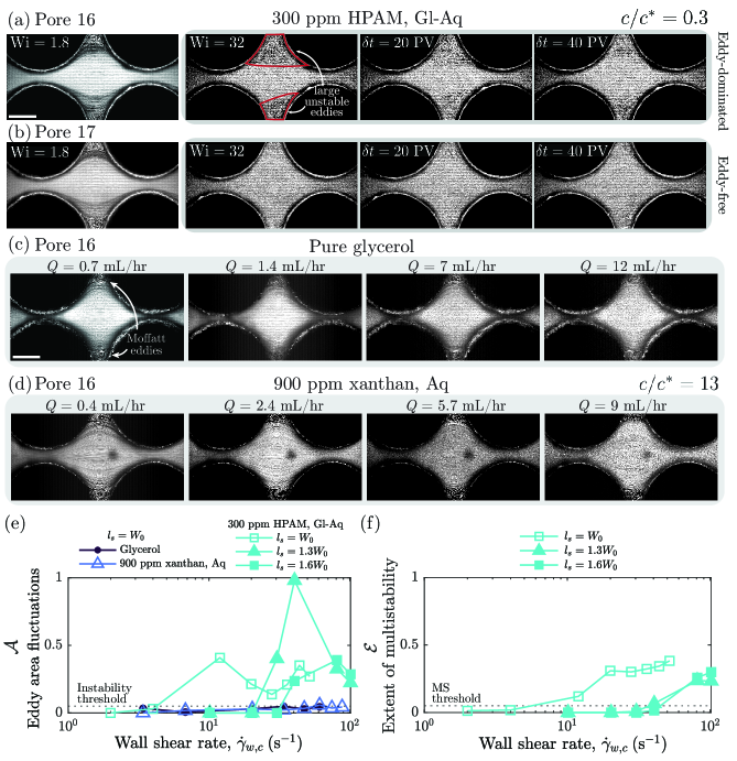
Figure 4: Multistability of a highly-elastic, non-shear-thinning fluid (300 ppm HPAM, Gl-Aq). (a–b) Streakline images of the flow, averaged over a duration of 5 pore volumes (PVs), in pore bodies (a) 16 and (b) 17 at two different Weissenberg numbers, $\mathrm{Wi}=1.8$ (leftmost column) and $\mathrm{Wi}=32$ (right three columns showing three different time points separated by $\delta t=20$ PV). Scale bar represents 500 $\mathrm{\upmu m}$. At $\mathrm{Wi}=1.8$, the flow in both pores is laminar, with stable Moffatt eddies in the corners of the pore bodies. At $\mathrm{Wi}=32$, the flow is highly unstable, as shown by the crossing streaklines. During the imaging period, pore 16 is “eddy-dominated”, with large fluctuating eddies located in the top and bottom corners of the pore body (outlined in red). At the same imposed flow rate, pore 17 is also unstable but exhibits nearly “eddy-free” behavior, with crossing streaklines filling more of the pore area. We term this finding that distinct pores exhibit distinct unstable flow states “multistability”. (c-d) Streakline images of the flow of (c) glycerol and (d) xanthan solutions in pore body 16 over similar ranges of flow rates show laminar flow with constant Moffatt eddies in the corners of pore bodies, indicating that fluid elasticity is necessary for instability to occur. (e) We quantify the onset of unstable flow using the root-mean-square temporal fluctuations in the size of each eddy, $A^{\prime}_{\mathrm{eddy,rms}}$, normalized by the mean value, $\langle A_{\mathrm{eddy}}\rangle_{t}$, aggregated for all imaged pores: $\mathcal{A}\equiv A^{\prime}_{\mathrm{eddy,rms}}/\langle A_{\mathrm{eddy}}\rangle_{t}$. We characterize the flow as being unstable when $\mathcal{A}$ exceeds a threshold value $0.05$, determined from noise in eddy area measurements of glycerol and xanthan gum controls solutions that remain laminar. (f) We quantify the extent of multistability using the difference between the maximal and minimal observed eddy size, normalized by the size of a pore body: $\mathcal{E}\equiv\left(\mathrm{max}\{A_{\mathrm{eddy}}\}-\mathrm{min}\{A_{\mathrm{eddy}}\}\right)/A_{\mathrm{pore}}$. The onset of both unstable flow, and multistability, are pushed to higher shear rates as the pore constriction spacing increases.

Even though all the pore constrictions in the array are fabricated to be geometrically identical, the features of the unstable flow differ from pore to pore. In particular, consistent with our previous findings Browne, Shih, and Datta (2020a), individual pore bodies exhibit one of two distinct unstable flow states, each of which persists over long durations—a phenomenon we term multistability—as exemplified by the righthand panels in Figs. 4(a–b) and in Supplementary Movie 1. Pore body 16 [top row] is “eddy-dominated” during the imaging period: large, fluctuating eddies [red outlines] form and persist in the corners between pore constrictions. Pore body 17 [bottom row] is instead “eddy-free”: the fluctuating fluid pathlines fill most of the pore space and eddies do not persist in all corners between constrictions. We quantify this behavior by measuring the difference between the maximal and minimal observed eddy size, normalized by the size of a pore body: $\mathcal{E}\equiv\left(\mathrm{max}\{A_{\mathrm{eddy}}\}-\mathrm{min}\{A_{\mathrm{eddy}}\}\right)/A_{\mathrm{pore}}$, which characterizes the extent of multistability. As shown by the open square symbols in Fig. 4(f), multistability arises concomitant with the onset of unstable flow at a constriction wall shear rate $\dot{\gamma}_{w,c}\sim 4-10\>\mathrm{s^{-1}}$, corresponding to $\mathrm{Wi}\sim 2-6$ and $\mathrm{M}\sim 6-19$.

Simulations Kumar et al. (2021) indicate that this unusual behavior arises from the competition between flow-induced polymer elongation, which promotes eddy formation Batchelor (1971); Boger (1987); Mongruel and Cloitre (1995, 2003); Rodd et al. (2007), and relaxation of polymers as they are advected between pore constrictions, causing elastic stresses to dissipate and enabling the eddy-free state to form. To test this idea, we increase $l_{s}$, providing more time for elastic stresses to relax as fluid is advected between constrictions. In this case, we expect that the onset of multistability is suppressed and shifted to higher shear rates. Repeating our experiments for $l_{s}=1.3W_{0}$ and $1.6W_{0}$ confirms this expectation. The elastic instability arises at $\dot{\gamma}_{w,c}\sim 20-30\>\mathrm{s^{-1}}$ ($\mathrm{Wi}\sim 11-17$, $\mathrm{M}\sim 17-26$) and $\dot{\gamma}_{w,c}\sim 30-40\>\mathrm{s^{-1}}$ ($\mathrm{Wi}\sim 17-24$, $\mathrm{M}\sim 26-35$) for $l_{s}=1.3W_{0}$ and $1.6W_{0}$, respectively, as shown by the filled triangles and squares in Fig. 4(c). Correspondingly, multistability arises only above $\dot{\gamma}_{w,c}\sim 30-40\>\mathrm{s^{-1}}$ ($\mathrm{Wi}\sim 55-73$, $\mathrm{M}17-24$) and $\dot{\gamma}_{w,c}\sim 40-80\>\mathrm{s^{-1}}$ ($\mathrm{Wi}\sim 73-140$, $\mathrm{M}\sim 24-52$) for $l_{s}=1.3W_{0}$ and $1.6W_{0}$, respectively, as shown by the filled triangles and squares in Fig. 4(d). Furthermore, repeating these experiments for another highly-elastic but non-shear-thinning fluid, but with a different solvent (300 ppm HPAM, Gl-Aq-DMSO—red square in Fig. 3), yields similar results [summarized in Fig. 6 for brevity]—indicating that our findings are more general.

III.2 Influence of shear-thinning on multistability

To investigate how fluid shear-thinning may influence the onset and features of this multistability, we next repeat the same experiments, but with different elastic fluids of systematically-varying degrees of shear-thinning.

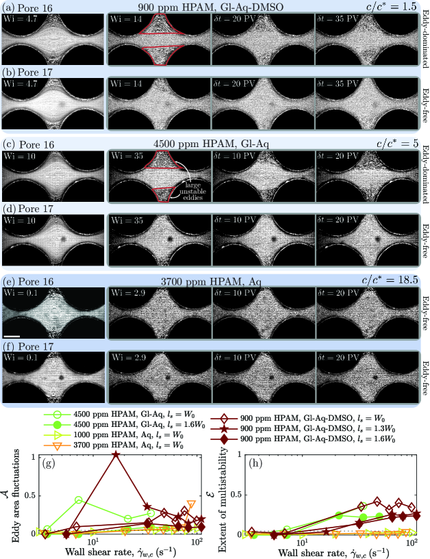
Figure 5: Multistability of fluids with different rheological properties. (a–f) Streakline images of the flow, averaged over 5 PVs, in pore bodies 16 and 17 at two different Weissernberg numbers, for (a–b) moderately shear-thinning and highly-elastic 900 ppm HPAM, Gl-Aq-DMSO, (c–d) highly shear-thinning and elastic 4500 ppm HPAM, Gl-Aq, and (e–f) highly shear-thinning and moderately-elastic 3700 ppm HPAM, Aq. Scale bar represents 500 $\mathrm{\upmu m}$. The leftmost column corresponds to sufficiently small Wi such that the flow is laminar. The righthand three columns show the unstable flow at three different time points. In (a–b) and (c–d), the flow is multistable, as in Fig. 4. By contrast, in (e–f), the flow is unstable, but is primarily “eddy-free”. (g) Onset of unstable flow characterized again using the measure of eddy size fluctuations $\mathcal{A}\equiv A^{\prime}_{\mathrm{eddy,rms}}/\langle A_{\mathrm{eddy}}\rangle_{t}$. (h) Onset of multistability characterized again using the measure of eddy size variations $\mathcal{E}\equiv\left(\mathrm{max}\{A_{\mathrm{eddy}}\}-\mathrm{min}\{A_{\mathrm{eddy}}\}\right)/A_{\mathrm{pore}}$.

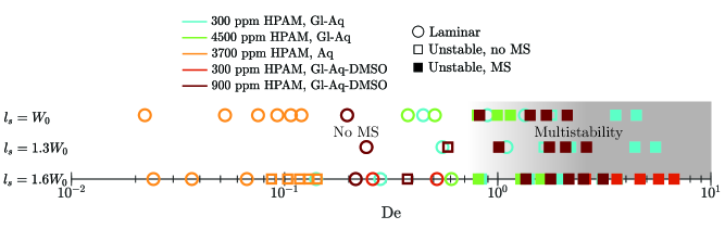
Figure 6: Streamwise Deborah number parameterizes the onset of multistability. The data show all our measurements across different flow rates, test fluids of varying rheological properties, and medium geometries of varying pore constriction spacings. The Deborah number is defined as $\mathrm{De}=\lambda/t_{\mathrm{adv}}$, where $\lambda$ is a rate-dependent relaxation time and $t_{\mathrm{adv}}$ is the characteristic time for fluid to be advected between pore constrictions, as described in the main text. Open circles indicate experiments where the flow is laminar; open squares indicate experiments where the flow is unstable, but does not exhibit multistability; filled squares indicates experiments where the flow is both unstable and multistable. Across all experiments, the transition to multistability occurs at $\mathrm{De}\sim 1$.

First, we test a higher concentration (900 ppm) of HPAM dissolved in the same Gl-Aq-DMSO solvent (crimson circle in Fig. 3). Unlike the dilute case of §III.1, this solution is semi-dilute ($c/c^{*}\approx 1.5$). The increased amount of polymer imparts further elasticity to the solution, and importantly, renders it moderately shear-thinning, as shown by the crimson point in Fig. 3. Notably, this added shear-thinning does not abrogate multistability (Supplementary Movie 2). An example is shown in Fig. 5(a–b): Pore body 16 [top row] is in the eddy-dominated unstable state, while pore body 17 [bottom row] is simultaneously in the eddy-free unstable state. Following §III.1, we characterize this behavior by measuring the extent of unstable flow and multistability, $\mathcal{A}$ and $\mathcal{E}$, respectively, over a range of flow rates and for devices with varying pore constriction spacings. We find similar behavior to the cases described in §III.1, as shown by the crimson points in Fig. 5(g–h). For $l_{s}=W_{0}$, the elastic instability arises at $\dot{\gamma}_{w,c}\sim 4-7\>\mathrm{s^{-1}}$ ($\mathrm{Wi}\sim 5-6$, $\mathrm{M}\sim 19-31$) and multistability correspondingly arises above $\dot{\gamma}_{w,c}\sim 7-34\>\mathrm{s^{-1}}$ ($\mathrm{Wi}\sim 6-10$, $\mathrm{M}\sim 31-89$). Consistent with the idea that multistability arises when flow-induced polymer elongation is faster than the relaxation of polymers as they are advected between pore constrictions, this threshold is again shifted to larger shear rates with increasing $l_{s}$.

Next, we examine the generality of these findings—that shear-thinning does not abrogate multistability, which arises when polymers are stretched faster than they can relax between pore constrictions—by testing another highly shear-thinning and elastic semi-dilute polymer solution. In particular, we test the same Gl-Aq solution as the starting case of §III.1, but at a higher concentration of 4500 ppm HPAM ($c/c^{*}\approx 5$, green circle in Fig. 3), over a range of flow rates and pore constriction spacings. We again find similar behavior to the cases described in §III.1 and the case of 900 ppm HPAM, Gl-Aq-DMSO shown in Fig. 5(a–b). Two exemplary pores are shown in Fig. 5(c–d) and Supplementary Movie 1, and the aggregated measurements of $\mathcal{A}$ and $\mathcal{E}$ characterizing the extent of unstable flow and multistability are shown by the green points in Fig. 5(g–h). As before, for sufficiently large shear rates, the flow becomes unstable and exhibits multistability. Moreover, this threshold is again shifted to larger shear rates as $l_{s}$ increases, further supporting the picture proposed in Refs. Browne, Shih, and Datta (2020a); Kumar et al. (2021).

Finally, we test two shear-thinning but less elastic fluids. One is formulated by maintaining the same relative concentration $c/c^{*}\approx 5$ in the semidilute, unentangled regime, but with the polymer dissolved in ultrapure water, which acts as a higher-quality solvent (1000 ppm HPAM, Aq). The other is formulated using an even higher polymer concentration in the entangled regime ($c/c^{*}\approx 19$), again in ultrapure water (3700 ppm HPAM, Aq—orange star in Fig. 3). In this case, based on the picture proposed in Refs. Browne, Shih, and Datta (2020a); Kumar et al. (2021), we expect that multistability will be suppressed because the characteristic solution relaxation times are reduced [Fig. 2(e) and Table 1]. Our experiments confirm this expectation (Supplementary Movie 2). Two exemplary pores are shown in Fig. 5(e–f), and the aggregated measurements of $\mathcal{A}$ and $\mathcal{E}$ characterizing the extent of unstable flow and multistability are shown by the yellow and orange points in Fig. 5(g–h). As before, for sufficiently large shear rates, the flow becomes unstable; however, it does not become multistable. Instead, all pores show the same behavior—the corner eddies become progressively smaller with increasing shear rate, and the flow exhibits strong spatiotemporal fluctuations throughout the pore body similar to the “eddy-free” case—even at the largest shear rates and smallest pore constriction spacings.

III.3 Streamwise Deborah number captures the onset of multistability

Taken altogether, the experiments described in §III.1–III.2 demonstrate that shear-thinning does not abrogate the onset of the elastic instability and the resulting development of multistability. Moreover, we find no correlation between the onset of multistability and standard physicochemical descriptors of polymer solutions: the degree of shear-thinning $S_{\textrm{max}}$, relative concentration regime $c/c^{*}$, solvent quality, zero-shear viscosity $\eta_{0}$, or the solvent contribution to the total viscosity $\beta$. Instead, guided by the picture proposed in Refs. Browne, Shih, and Datta (2020a); Kumar et al. (2021), we examine whether the streamwise Deborah number $\mathrm{De}=\lambda/t_{\mathrm{adv}}$ can capture the onset of multistability. We calculate the characteristic time for fluid to be advected between pore constrictions as $t_{\mathrm{adv}}=V_{\mathrm{pore}}/Q$. Importantly, unlike in our previous work Browne, Shih, and Datta (2020a), here, the solution stress relaxation time $\lambda$ incorporates shear-thinning rheology through its rate dependence, as described in §II.3. Specifically, for the non-shear-thinning solutions, we take $\lambda=\lambda_{0}$, the longest stress relaxation time, as in previous work  Boger (1987); James (2009); this choice quantifies the expectation that for these solutions, the longest relaxation time corresponding to relaxation of an entire polymer chain governs stress relaxation Bird, Armstrong, and Hassager (1987); Rubinstein and Colby (2003); Morozov and Van Saarloos (2007); Larson and Desai (2015). By contrast, for the shear-thinning fluids, we evaluate the relaxation time as $\lambda=\lambda_{\mathrm{WM}}(\dot{\gamma}_{w,c})$ at each flow rate tested; this choice quantifies the expectation that these solutions have multiple modes of stress relaxation that are coupled to flow-induced microstructural rearrangements De Gennes (1971); Rubinstein and Colby (2003); Litvinov, Hu, and Adams (2011); Klebinger, Wunderlich, and Bausch (2013); Howe, Clarke, and Giernalczyk (2015); Larson and Desai (2015).

All of our results—across eight different test fluids of systematically-varying rheological properties and three different pore constriction spacings—are summarized by the state diagram shown in Fig. 6. Remarkably, despite the complex nature of the elastic instability, all of our results show excellent collapse when parameterized by $\mathrm{De}$. When $\mathrm{De}<1$, we do not observe multistability (open symbols): the flow is either laminar, or with all pores exhibiting similar unstable “eddy-free” flow. By contrast, when $\mathrm{De}$ exceeds a threshold value $\mathcal{O}(1)$, the flow is multistable (closed symbols). This collapse therefore demonstrates that the picture proposed by Refs. Browne, Shih, and Datta (2020a); Kumar et al. (2021)—that multistability arises when flow-induced polymer elongation is faster than polymer relaxation between adjacent pore constrictions—holds across a diverse array of fluids with varying rheological properties.

IV Conclusion

In summary, using flow visualization in microfabricated millifluidic devices, we have investigated the influence of systematic variations in fluid shear-thinning or elasticity on the unstable flow of polymer solutions in 1D ordered arrays of pore constrictions. In all cases, when the fluid is sufficiently elastic, it exhibits a flow instability above a threshold flow rate; intriguingly, the parameters $\mathrm{Wi}$ and $\mathrm{M}$ do not appear to uniquely capture the onset of this unstable flow across the different solutions and device geometries. However, the parameter $\mathrm{De}$ — which compares the shear rate-dependent longest stress relaxation time to the advection time between pores — captures the onset of multistability in the unstable flow across all our experiments. Our work thereby demonstrates that the picture proposed in Refs. Browne, Shih, and Datta (2020a); Kumar et al. (2021) holds more broadly, and corroborates other studies suggesting that the rate-dependence of polymer relaxation can influence elastic instabilities Casanellas et al. (2016); Shakeri, Jung, and Seemann (2022b).

Our experiments explored polymer solutions of varying concentrations, solvent qualities, and viscosities, primarily using the same high molecular weight HPAM. In future work, it will be useful to investigate variations in the polymer molecular weight, architecture, and composition to further explore the general applicability of our findings. It will also be useful to examine different definitions of the streamwise Deborah number — for example, using shear stress relaxation times determined using other approaches than that used here Del Giudice, Haward, and Shen (2017); Souliès et al. (2017); Khalkhal and Muller (2022, 2022) or, given the central role of polymer extension in determining the characteristics of the unstable flow behavior, using an extensional relaxation time Klebinger, Wunderlich, and Bausch (2013); Larson and Desai (2015) determined using e.g., capillary breakup rheometry McKinley (2005), cross slot rheometry Haward et al. (2012, 2023a, 2023b), or dripping-on-substrate rheometry Dinic, Jimenez, and Sharma (2017).

Altogether, by deepening understanding of the influence of fluid rheology on elastic instabilities, our work helps to pave the way towards the rational tuning of both fluid rheology Ewoldt and Saengow (2022) and porous medium geometry Stone, Stroock, and Ajdari (2004) to harness such instabilities in diverse chemical, energy, environmental, and industrial settings—for example, using them to enhance heat/mass transport in porous media Groisman and Steinberg (2001); Traore, Castelain, and Burghelea (2015); Whalley et al. (2015); Browne et al. (2023); Kumar et al. (2023); Browne and Datta (2023), where eddy-dominated pores could act as semi-compartmentalized microreactors Trojanowicz (2020).

SI Movie Captions

SI Movie 1. Comparison of laminar and unstable flow behavior in the $l_{s}=1W_{0}$ 1-D pore array. (a-b) Streakline imaging of the flow of the weakly shear-thinning, highly elastic 300 ppm HPAM, Gl-Aq solution in pore body 16 showing (a) laminar (Wi = 1.8 $<$ Wi${}_{c}\approx 6$) and (b) unstable (Wi = 26 $>$ Wi${}_{c}\approx 6$) flow behavior. Flow is from left to right. (c-d) Streakline imaging of the flow of the highly shear-thinning, highly elastic 4500 ppm HPAM, Gl-Aq solution showing (c) laminar (Wi = 10 $<$ Wi${}_{c}\approx 15$) and (d) unstable (Wi = 34 $>$ Wi${}_{c}\approx 15$) flow behavior. Unstable flow behavior is visualized by crossing streaklines and fluctuations in the eddy sizes. Both solutions exhibit multistability in the unstable flow state, as described in the main text; thus, shear-thinning does not abrogate multistability. The movies shown correspond to an “eddy-dominated” pore over the imaging window. Streaklines are generated using a moving average of the fluorescence intensity of tracer particles over 30 successive frames. Scale bar is $500\>\upmu$m. Videos play at 15x real time.

SI Movie 2. Comparison of multistable and non-multistable flow behavior above the onset of elastic instability (Wi $>$ Wi_c) for polymer solutions in the $l_{s}=1W_{0}$ 1-D pore array. (a-c) Unstable flow exhibiting multistability for the moderately shear-thinning, highly elastic 900 ppm HPAM, Gl-Aq-DMSO solution in three consecutive pore bodies. Pore bodies 15 and 16 appear eddy-dominated over the imaging window, while pore body 17 transitions between eddy-dominated and eddy-free states. Flow is from left to right. (d-f) Unstable flow showing no multistability for the highly shear-thinning, moderately elastic 3700 ppm HPAM, Aq solution. The unstable flow is observed qualitatively by crossing streaklines in the bulk of the pore body and fluctuations of the small corner eddies. However, all pore bodies exhibit the same instability flow behavior at the same imposed flow rate, showing a lack of multistability. Imaging is recorded sequentially in adjacent pores, producing a time offset of 2 minutes from pore-to-pore. Streaklines are generated using a moving average of the fluorescence intensity of tracer particles over 30 successive frames. Scale bar is $500\>\upmu$m. Videos play at 15x real time.

Author Contributions

E.Y.C. and S.S.D. designed the experiments; E.Y.C. performed all experiments; E.Y.C. and S.S.D. analyzed all data, discussed the results and implications, and wrote the manuscript; and S.S.D. designed and supervised the overall project.

Conflict of Interest Statement

There are no conflicts of interest to declare.

Data Availability Statement

All data, and description of all methods required to reproduce the results, are completely included in the manuscript and/or supporting information.

References

- Kozicki and Slegr (1994) W. Kozicki and H. Slegr, “Filtration in viscoelastic continua,” J. Non-Newton. Fluid Mech. 53, 129–149 (1994).
- Luo and Teraoka (1996) M. Luo and I. Teraoka, “High Osmotic Pressure Chromatography for Large-Scale Fractionation of Polymers,” Macromolecules 29, 4226–4233 (1996).
- Bourgeat, Gipouloux, and Marusic-Paloka (2003) A. Bourgeat, O. Gipouloux, and E. Marusic-Paloka, “Filtration Law for Polymer Flow Through Porous Media,” Multiscale Model. Simul. 1, 432–457 (2003).
- Petrie and Denn (1976) C. J. S. Petrie and M. M. Denn, “Instabilities in polymer processing,” AIChE J 22, 209–236 (1976).
- Denn (2008) M. M. Denn, Polymer Melt Processing: Foundations in Fluid Mechanics and Heat Transfer (Cambridge University Press, 2008).
- Turner, Strong, and Gold (2014) B. N. Turner, R. Strong, and S. A. Gold, “A review of melt extrusion additive manufacturing processes: I. Process design and modeling,” Rapid Protyp. J. 20, 192–204 (2014).
- Elbadawi (2018) M. Elbadawi, “Polymeric Additive Manufacturing: The Necessity and Utility of Rheology,” in Polymer Rheology (InTechOpen, 2018).
- Durst, Haas, and Kaczmar (1981) F. Durst, R. Haas, and B. U. Kaczmar, “Flows of dilute hydrolyzed polyacrylamide solutions in porous media under various solvent conditions,” J. Appl. Polym. Sci. 26, 3125–3149 (1981).
- Seright et al. (2010) R. S. Seright, T. Fan, K. Wavrik, and R. d. C. Balaban, “New Insights into Polymer Rheology in Porous Media,” Soc. Pet. Eng. J. (2010).
- Sorbie (2013) K. S. Sorbie, Polymer-Improved Oil Recovery, 1st ed. (Springer Dordrecht, 2013).
- Clarke et al. (2016) A. Clarke, A. M. Howe, J. Mitchell, J. Staniland, and L. A. Hawkes, “How Viscoelastic-Polymer Flooding Enhances Displacement Efficiency,” SPE J. 21, 675–687 (2016).
- Pogaku et al. (2018) R. Pogaku, N. H. Mohd Fuat, S. Sakar, Z. W. Cha, N. Musa, D. N. A. Awang Tajudin, and L. O. Morris, “Polymer flooding and its combinations with other chemical injection methods in enhanced oil recovery,” Polym. Bull. 75, 1753–1774 (2018).
- Mirzaie Yegane, Boukany, and Zitha (2022) M. Mirzaie Yegane, P. E. Boukany, and P. Zitha, “Fundamentals and Recent Progress in the Flow of Water-Soluble Polymers in Porous Media for Enhanced Oil Recovery,” Energies 15 (2022), 10.3390/en15228575.
- Roote (1998) D. S. Roote, “Technology Status Report: In Situ Flushing,” Tech. Rep. (Ground-Water Remediation Technologies Analysis Center, 1998).
- Smith et al. (2008) M. M. Smith, J. A. K. Silva, J. Munakata-Marr, and J. E. McCray, “Compatibility of Polymers and Chemical Oxidants for Enhanced Groundwater Remediation,” Environ. Sci. Technol. 42, 9296–9301 (2008).
- Huo et al. (2020) L. Huo, G. Liu, X. Yang, Z. Ahmad, and H. Zhong, “Surfactant-enhanced aquifer remediation: Mechanisms, influences, limitations and the countermeasures,” Chemosphere 252 (2020), https://doi.org/10.1016/j.chemosphere.2020.126620.
- Hartmann et al. (2021) A. Hartmann, S. Jasechko, T. Gleeson, Y. Wada, B. Andreo, J. A. Barberá, H. Brielmann, L. Bouchaou, J.-B. Charlier, W. G. Darling, M. Filippini, J. Garvelmann, N. Goldscheider, M. Kralik, H. Kunstmann, B. Ladouche, J. Lange, G. Lucianetti, J. F. Martín, M. Mudarra, D. Sánchez, C. Stumpp, E. Zagana, and T. Wagener, “Risk of groundwater contamination widely underestimated because of fast flow into aquifers,” Proc. Natl. Acad. Sci. U.S.A. 118 (2021), 10.1073/pnas.2024492118.
- Di Dato et al. (2022) M. Di Dato, C. D’Angelo, A. Casasso, and A. Zarlenga, “The impact of porous medium heterogeneity on the thermal feedback of open-loop shallow geothermal systems,” J. Hydrol. 604 (2022), 10.1016/j.jhydrol.2021.127205.
- Macosko (1994) C. W. Macosko, Rheology: principles, measurements, and applications, Advances in interfacial engineering series (VCH, New York, 1994).
- Larson (1999) R. G. Larson, The Structure and Rheology of Complex Fluids (Oxford University Press, 1999).
- Rubinstein and Colby (2003) M. Rubinstein and R. H. Colby, Polymer Physics (Oxford University Press, 2003).
- Ryder and Yeomans (2006) J. F. Ryder and J. M. Yeomans, “Shear thinning in dilute polymer solutions,” J. Chem. Phys. 125, 194906 (2006).
- Larson (1992) R. G. Larson, “Instabilities in viscoelastic flows,” Rheol. Acta 31, 213–263 (1992).
- McKinley, Pakdel, and Öztekin (1996) G. H. McKinley, P. Pakdel, and A. Öztekin, “Rheological and geometric scaling of purely elastic flow instabilities,” J. Non-Newton. Fluid Mech. 67, 19–47 (1996).
- Pakdel and McKinley (1996) P. Pakdel and G. H. McKinley, “Elastic Instability and Curved Streamlines,” Phys. Rev. Lett. 77, 2459–2462 (1996).
- Weissenberg (1947) K. Weissenberg, “A continuum theory of rheological phenomena,” Nature (1947).
- Bird, Armstrong, and Hassager (1987) R. B. Bird, R. C. Armstrong, and O. Hassager, Dynamics of Polymeric Liquids: Kinetic Theory, Vol. 2 (Wiley Interscience, 1987).
- More et al. (2023) R. V. More, R. Patterson, E. Pashkovski, and G. H. McKinley, “Rod-climbing rheometry revisited,” Soft Matter (2023).
- Datta et al. (2022) S. S. Datta, A. M. Ardekani, P. E. Arratia, A. N. Beris, I. Bischofberger, G. H. McKinley, J. G. Eggers, J. E. López-Aguilar, S. M. Fielding, A. Frishman, M. D. Graham, J. S. Guasto, S. J. Haward, A. Q. Shen, S. Hormozi, A. Morozov, R. J. Poole, V. Shankar, E. S. G. Shaqfeh, H. Stark, V. Steinberg, G. Subramanian, and H. A. Stone, “Perspectives on viscoelastic flow instabilities and elastic turbulence,” Phys. Rev. Fluids 7 (2022), 10.1103/PhysRevFluids.7.080701.
- Pearson (1976) J. R. A. Pearson, “Instability in Non-Newtonian Flow,” Annual Review of Fluid Mechanics (1976).
- Shaqfeh (1996) E. S. G. Shaqfeh, “Purely Elastic Instabilities in Viscometric Flows,” Annu. Rev. Fluid Mech. 28, 129–185 (1996).
- Groisman and Steinberg (2001) A. Groisman and V. Steinberg, “Efficient mixing at low Reynolds numbers using polymer additives,” Nature 410 (2001).
- Ducloué et al. (2019) L. Ducloué, L. Casanellas, S. J. Haward, R. J. Poole, M. A. Alves, S. Lerouge, A. Q. Shen, and A. Lindner, “Secondary flows of viscoelastic fluids in serpentine microchannels,” Microfluid Nanofluid 23, 33 (2019).
- Shakeri, Jung, and Seemann (2022a) P. Shakeri, M. Jung, and R. Seemann, “Characterizing purely elastic turbulent flow of a semi-dilute entangled polymer solution in a serpentine channel,” Phys. Fluids 34 (2022a), 10.1063/5.0100419.
- Batchelor (1971) G. K. Batchelor, “The stress generated in a non-dilute suspension of elongated particles by pure straining motion,” J. Fluid Mech. 46, 813–829 (1971).
- Boger (1987) D. V. Boger, “Viscoelastic Flows Through Contractions,” Annu. Rev. Fluid Mech. 19 (1987).
- Koelling and Prud’homme (1991) K. W. Koelling and R. K. Prud’homme, “Instabilities in multi-hole converging flow of viscoelastic fluids,” Rheol Acta 30, 511–522 (1991).
- Byars et al. (1994) J. A. Byars, A. Öztekin, R. A. Brown, and G. H. Mckinley, “Spiral instabilities in the flow of highly elastic fluids between rotating parallel disks,” J. Fluid Mech. 271, 173–218 (1994).
- Mongruel and Cloitre (1995) A. Mongruel and M. Cloitre, “Extensional flow of semidilute suspensions of rod-like particles through an orifice,” Phys. Fluids 7, 2546–2552 (1995).
- Khomami and Moreno (1997) D. B. Khomami and L. D. Moreno, “Stability of viscoelastic flow around periodic arrays of cylinders,” Rheol. Acta 36 (1997).
- Arora, Sureshkumar, and Khomami (2002) K. Arora, R. Sureshkumar, and B. Khomami, “Experimental investigation of purely elastic instabilities in periodic flows,” J. Non-Newton. Fluid Mech. 108, 18 (2002).
- Mongruel and Cloitre (2003) A. Mongruel and M. Cloitre, “Axisymmetric orifice flow for measuring the elongational viscosity of semi-rigid polymer solutions,” J. Non-Newton. Fluid Mech. 110, 27–43 (2003).
- Groisman and Steinberg (2000) A. Groisman and V. Steinberg, “Elastic turbulence in a polymer solution flow,” Nature 405 (2000).
- Rodd et al. (2007) L. Rodd, J. Cooper-White, D. Boger, and G. McKinley, “Role of the elasticity number in the entry flow of dilute polymer solutions in micro-fabricated contraction geometries,” J. Non-Newton. Fluid Mech. 143, 170–191 (2007).
- Lanzaro and Yuan (2011) A. Lanzaro and X.-F. Yuan, “Effects of contraction ratio on non-linear dynamics of semi-dilute, highly polydisperse PAAm solutions in microfluidics,” J. Non-Newton. Fluid Mech. 166, 1064–1075 (2011).
- Kenney et al. (2013) S. Kenney, K. Poper, G. Chapagain, and G. F. Christopher, “Large Deborah number flows around confined microfluidic cylinders,” Rheol Acta 52, 485–497 (2013).
- Gulati, Muller, and Liepmann (2015) S. Gulati, S. J. Muller, and D. Liepmann, “Flow of DNA solutions in a microfluidic gradual contraction,” Biomicrofluidics 9, 054102 (2015).
- Shi and Christopher (2016) X. Shi and G. F. Christopher, “Growth of viscoelastic instabilities around linear cylinder arrays,” Phys. Fluids 28 (2016), 10.1063/1.4968221.
- Varshney and Steinberg (2017) A. Varshney and V. Steinberg, “Elastic wake instabilities in a creeping flow between two obstacles,” Phys. Rev. Fluids 2 (2017), 10.1103/PhysRevFluids.2.051301.
- Qin et al. (2019) B. Qin, P. F. Salipante, S. D. Hudson, and P. E. Arratia, “Upstream vortex and elastic wave in the viscoelastic flow around a confined cylinder,” J. Fluid Mech. 864 (2019), 10.1017/jfm.2019.73.
- Hopkins, Haward, and Shen (2022) C. C. Hopkins, S. J. Haward, and A. Q. Shen, “Upstream wall vortices in viscoelastic flow past a cylinder,” Soft Matter 18, 4868–4880 (2022).
- Sousa, Pinho, and Alves (2018) P. C. Sousa, F. T. Pinho, and M. A. Alves, “Purely-elastic flow instabilities and elastic turbulence in microfluidic cross-slot devices,” Soft Matter 14, 1344–1354 (2018).
- Hopkins, Haward, and Shen (2020) C. C. Hopkins, S. J. Haward, and A. Q. Shen, “Purely Elastic Fluid–Structure Interactions in Microfluidics: Implications for Mucociliary Flows,” Small 16 (2020), 10.1002/smll.201903872.
- Kawale et al. (2017a) D. Kawale, E. Marques, P. L. J. Zitha, M. T. Kreutzer, W. R. Rossen, and P. E. Boukany, “Elastic instabilities during the flow of hydrolyzed polyacrylamide solution in porous media: effect of pore-shape and salt,” Soft Matter 13, 765–775 (2017a).
- Kawale et al. (2017b) D. Kawale, G. Bouwman, S. Sachdev, P. L. J. Zitha, M. T. Kreutzer, W. R. Rossen, and P. E. Boukany, “Polymer conformation during flow in porous media,” Soft Matter 13, 8745–8755 (2017b).
- Kawale, Jayaraman, and Boukany (2019) D. Kawale, J. Jayaraman, and P. E. Boukany, “Microfluidic rectifier for polymer solutions flowing through porous media,” Biomicrofluidics 13 (2019), 10.1063/1.5050201.
- Ichikawa and Motosuke (2022) Y. Ichikawa and M. Motosuke, “Viscoelastic flow behavior and formation of dead zone around triangle-shaped pillar array in microchannel,” Microfluid Nanofluid 26 (2022), 10.1007/s10404-022-02549-9.
- Arratia et al. (2006) P. E. Arratia, C. C. Thomas, J. Diorio, and J. P. Gollub, “Elastic Instabilities of Polymer Solutions in Cross-Channel Flow,” Phys. Rev. Lett. 96 (2006), 10.1103/PhysRevLett.96.144502.
- Galindo-Rosales, Oliveira, and Alves (2014) F. J. Galindo-Rosales, M. S. N. Oliveira, and M. A. Alves, “Optimized cross-slot microdevices for homogeneous extension,” RSC Adv. 4, 7799 (2014).
- Ribeiro et al. (2014) V. Ribeiro, P. Coelho, F. Pinho, and M. Alves, “Viscoelastic fluid flow past a confined cylinder: Three-dimensional effects and stability,” Chem. Eng. Sci. 111, 364–380 (2014).
- Haward, McKinley, and Shen (2016) S. J. Haward, G. H. McKinley, and A. Q. Shen, “Elastic instabilities in planar elongational flow of monodisperse polymer solutions,” Sci Rep 6, 33029 (2016).
- Lanzaro, Corbett, and Yuan (2017) A. Lanzaro, D. Corbett, and X.-F. Yuan, “Non-linear dynamics of semi-dilute PAAm solutions in a microfluidic 3D cross-slot flow geometry,” J. Non-Newton. Fluid Mech. 242, 57–65 (2017).
- Haward, Toda-Peters, and Shen (2018) S. J. Haward, K. Toda-Peters, and A. Q. Shen, “Steady viscoelastic flow around high-aspect-ratio, low-blockage-ratio microfluidic cylinders,” J. Non-Newton. Fluid Mech. 254, 23–35 (2018).
- Davoodi, Domingues, and Poole (2019) M. Davoodi, A. F. Domingues, and R. J. Poole, “Control of a purely elastic symmetry-breaking flow instability in cross-slot geometries,” J. Fluid Mech. 881, 1123–1157 (2019).
- Qin et al. (2020) B. Qin, R. Ran, P. F. Salipante, S. D. Hudson, and P. E. Arratia, “Three-dimensional structures and symmetry breaking in viscoelastic cross-channel flow,” Soft Matter 16, 6969–6974 (2020).
- Yokokoji et al. (2023) A. Yokokoji, S. Varchanis, A. Q. Shen, and S. J. Haward, “Rheological effects on purely-elastic flow asymmetries in the cross-slot geometry,” Soft Matter (2023), 10.1039/D3SM01209C.
- Kumar et al. (2023) M. Kumar, D. M. Walkama, A. M. Ardekani, and J. S. Guasto, “Stress and stretching regulate dispersion in viscoelastic porous media flows,” Soft Matter (2023), 10.1039/D3SM00224A.
- Groisman and Steinberg (1998) A. Groisman and V. Steinberg, “Mechanism of elastic instability in Couette flow of polymer solutions: Experiment,” Phys. Fluids 10, 2451–2463 (1998).
- Pan et al. (2013) L. Pan, A. Morozov, C. Wagner, and P. E. Arratia, “Nonlinear Elastic Instability in Channel Flows at Low Reynolds Numbers,” Phys. Rev. Lett. 110, 174502 (2013).
- Scholz et al. (2014) C. Scholz, F. Wirner, J. R. Gomez-Solano, and C. Bechinger, “Enhanced dispersion by elastic turbulence in porous media,” EPL 107 (2014), 10.1209/0295-5075/107/54003.
- Clarke et al. (2015) A. Clarke, A. M. Howe, J. Mitchell, J. Staniland, L. Hawkes, and K. Leeper, “Mechanism of anomalously increased oil displacement with aqueous viscoelastic polymer solutions,” Soft Matter 11, 3536–3541 (2015).
- Howe, Clarke, and Giernalczyk (2015) A. M. Howe, A. Clarke, and D. Giernalczyk, “Flow of concentrated viscoelastic polymer solutions in porous media: effect of MW and concentration on elastic turbulence onset in various geometries,” Soft Matter 11, 6419–6431 (2015).
- Lanzaro, Li, and Yuan (2015) A. Lanzaro, Z. Li, and X.-F. Yuan, “Quantitative characterization of high molecular weight polymer solutions in microfluidic hyperbolic contraction flow,” Microfluid Nanofluid 18, 819–828 (2015).
- Traore, Castelain, and Burghelea (2015) B. Traore, C. Castelain, and T. Burghelea, “Efficient heat transfer in a regime of elastic turbulence,” J. Non-Newton. Fluid Mech. 223, 62–76 (2015).
- Whalley et al. (2015) R. Whalley, W. Abed, D. Dennis, and R. Poole, “Enhancing heat transfer at the micro-scale using elastic turbulence,” Theor. App. Mech. 5, 103–106 (2015).
- Mitchell et al. (2016) J. Mitchell, K. Lyons, A. M. Howe, and A. Clarke, “Viscoelastic polymer flows and elastic turbulence in three-dimensional porous structures,” Soft Matter 12, 460–468 (2016).
- Qin and Arratia (2017) B. Qin and P. E. Arratia, “Characterizing elastic turbulence in channel flows at low Reynolds number,” Phys. Rev. Fluids 2 (2017), 10.1103/PhysRevFluids.2.083302.
- Browne and Datta (2021) C. A. Browne and S. S. Datta, “Elastic turbulence generates anomalous flow resistance in porous media,” Sci. Adv. 7, 11 (2021).
- Shakeri, Jung, and Seemann (2021) P. Shakeri, M. Jung, and R. Seemann, “Effect of elastic instability on mobilization of capillary entrapments,” Phys. Fluids 33 (2021), 10.1063/5.0071556.
- Carlson et al. (2022) D. W. Carlson, K. Toda-Peters, A. Q. Shen, and S. J. Haward, “Volumetric evolution of elastic turbulence in porous media,” J. Fluid Mech. 950 (2022), 10.1017/jfm.2022.836.
- Browne et al. (2023) C. A. Browne, R. B. Huang, C. W. Zheng, and S. S. Datta, “Homogenizing fluid transport in stratified porous media using an elastic flow instability,” J. Fluid Mech. 963 (2023), 10.1017/jfm.2023.337.
- Browne and Datta (2023) C. A. Browne and S. S. Datta, “Harnessing elastic instabilities for enhanced mixing and reaction kinetics in porous media,” (2023), arXiv:2311.07431 [cond-mat, physics:nlin, physics:physics].
- James (2009) D. F. James, “Boger Fluids,” Annu. Rev. Fluid Mech. (2009).
- Larson, Muller, and Shaqfeh (1994) R. Larson, S. Muller, and E. Shaqfeh, “The effect of fluid rheology on the elastic Taylor-Couette instability,” J. Non-Newton. Fluid Mech. 51, 195–225 (1994).
- Jagdale et al. (2020) P. P. Jagdale, D. Li, X. Shao, J. B. Bostwick, and X. Xuan, “Fluid Rheological Effects on the Flow of Polymer Solutions in a Contraction–Expansion Microchannel,” Micromachines 11 (2020), 10.3390/mi11030278.
- Casanellas et al. (2016) L. Casanellas, M. A. Alves, R. J. Poole, S. Lerouge, and A. Lindner, “The stabilizing effect of shear thinning on the onset of purely elastic instabilities in serpentine microflows,” Soft Matter 12, 6167–6175 (2016).
- Cagney, Lacassagne, and Balabani (2020) N. Cagney, T. Lacassagne, and S. Balabani, “Taylor–Couette flow of polymer solutions with shear-thinning and viscoelastic rheology,” J. Fluid Mech. 905, A28 (2020).
- Lacassagne, Cagney, and Balabani (2021) T. Lacassagne, N. Cagney, and S. Balabani, “Shear-thinning mediation of elasto-inertial Taylor–Couette flow,” J. Fluid Mech. 915 (2021), 10.1017/jfm.2021.104.
- Browne, Shih, and Datta (2020a) C. A. Browne, A. Shih, and S. S. Datta, “Bistability in the unstable flow of polymer solutions through pore constriction arrays,” J. Fluid Mech. 890 (2020a), 10.1017/jfm.2020.122.
- Kumar et al. (2021) M. Kumar, S. Aramideh, C. A. Browne, S. S. Datta, and A. M. Ardekani, “Numerical investigation of multistability in the unstable flow of a polymer solution through porous media,” Phys. Rev. Fluids 6 (2021), 10.1103/PhysRevFluids.6.033304.
- Burghelea et al. (2004) T. Burghelea, E. Segre, I. Bar-Joseph, A. Groisman, and V. Steinberg, “Chaotic flow and efficient mixing in a microchannel with a polymer solution,” Phys. Rev. E 69 (2004), 10.1103/PhysRevE.69.066305.
- Pathak, Ross, and Migler (2004) J. A. Pathak, D. Ross, and K. B. Migler, “Elastic flow instability, curved streamlines, and mixing in microfluidic flows,” Phys. Fluids 16, 4028–4034 (2004).
- Dobrynin, Colby, and Rubinstein (1995) A. V. Dobrynin, R. H. Colby, and M. Rubinstein, “Scaling Theory of Polyelectrolyte Solutions,” Macromolecules 28, 1859–1871 (1995).
- Tran and Clarke (2023) E. Tran and A. Clarke, “The relaxation time of entangled HPAM solutions in flow,” J. Non-Newton. Fluid Mech. 311 (2023), 10.1016/j.jnnfm.2022.104954.
- Wyatt and Liberatore (2009) N. B. Wyatt and M. W. Liberatore, “Rheology and viscosity scaling of the polyelectrolyte xanthan gum,” J. Appl. Polym. Sci. 114, 4076–4084 (2009).
- Liu, Jun, and Steinberg (2009) Y. Liu, Y. Jun, and V. Steinberg, “Concentration dependence of the longest relaxation times of dilute and semi-dilute polymer solutions,” J. Rheol. 53, 1069–1085 (2009).
- Haward, Hopkins, and Shen (2020) S. J. Haward, C. C. Hopkins, and A. Q. Shen, “Asymmetric flow of polymer solutions around microfluidic cylinders: Interaction between shear-thinning and viscoelasticity,” J. Non-Newton. Fluid Mech. 278 (2020), 10.1016/j.jnnfm.2020.104250.
- Liu, Jun, and Steinberg (2007) Y. Liu, Y. Jun, and V. Steinberg, “Longest Relaxation Times of Double-Stranded and Single-Stranded DNA,” Macromolecules 40, 2172–2176 (2007).
- Shakeri, Jung, and Seemann (2022b) P. Shakeri, M. Jung, and R. Seemann, “Scaling purely elastic instability of strongly shear thinning polymer solutions,” Phys. Rev. E 105 (2022b), 10.1103/PhysRevE.105.L052501.
- White and Metzner (1963) J. L. White and A. B. Metzner, “Development of constitutive equations for polymeric melts and solutions,” J. Appl. Polym. Sci. 7, 1867–1889 (1963).
- Harnett (1989) J. P. Harnett, “Heat Transfer to Newtonian and Non-Newtonian Fluids in Rectangular Ducts,” in Advances in heat transfer, Vol. 19 (Academic Press, Inc., 1989) pp. 247–307.
- Son (2007) Y. Son, “Determination of shear viscosity and shear rate from pressure drop and flow rate relationship in a rectangular channel,” Polymer 48, 632–637 (2007).
- Morozov and Van Saarloos (2007) A. N. Morozov and W. Van Saarloos, “An introductory essay on subcritical instabilities and the transition to turbulence in visco-elastic parallel shear flows,” Physics Reports 447, 112–143 (2007).
- Larson and Desai (2015) R. Larson and P. S. Desai, “Modeling the Rheology of Polymer Melts and Solutions,” Annu. Rev. Fluid Mech. 47, 47–65 (2015).
- De Gennes (1971) P. G. De Gennes, “Reptation of a Polymer Chain in the Presence of Fixed Obstacles,” J. Chem. Phys. 55, 572–579 (1971).
- Litvinov, Hu, and Adams (2011) S. Litvinov, X. Y. Hu, and N. A. Adams, “Mesoscopic simulation of the transient behavior of semi-diluted polymer solution in a microchannel following extensional flow,” J. Phys.: Condens. Matter 23 (2011), 10.1088/0953-8984/23/18/184118.
- Klebinger, Wunderlich, and Bausch (2013) U. A. Klebinger, B. K. Wunderlich, and A. R. Bausch, “Transient flow behavior of complex fluids in microfluidic channels,” Microfluid Nanofluid 15, 533–540 (2013).
- Del Giudice, Haward, and Shen (2017) F. Del Giudice, S. J. Haward, and A. Q. Shen, “Relaxation time of dilute polymer solutions: A microfluidic approach,” J. Rheol. 61, 327–337 (2017).
- Souliès et al. (2017) A. Souliès, J. Aubril, C. Castelain, and T. Burghelea, “Characterisation of elastic turbulence in a serpentine micro-channel,” Phys. Fluids 29 (2017), 10.1063/1.4996356.
- Khalkhal and Muller (2022) F. Khalkhal and S. J. Muller, “Analyzing flow behavior of shear-thinning fluids in a planar abrupt contraction/expansion microfluidic geometry,” Phys. Rev. Fluids (2022).
- McKinley (2005) G. H. McKinley, “Visco-Elasto-Capillary Thinning and Break-Up of Complex Fluids,” Tech. Rep. 05-P-04 (2005).
- Haward et al. (2012) S. J. Haward, M. S. N. Oliveira, M. A. Alves, and G. H. McKinley, “Optimized Cross-Slot Flow Geometry for Microfluidic Extensional Rheometry,” Phys. Rev. Lett. 109 (2012), 10.1103/PhysRevLett.109.128301.
- Haward et al. (2023a) S. J. Haward, S. Varchanis, G. H. McKinley, M. A. Alves, and A. Q. Shen, “Extensional rheometry of mobile fluids. Part II: Comparison between the uniaxial, planar, and biaxial extensional rheology of dilute polymer solutions using numerically optimized stagnation point microfluidic devices,” J. Rheol. 67, 1011–1030 (2023a).
- Haward et al. (2023b) S. J. Haward, F. Pimenta, S. Varchanis, D. W. Carlson, K. Toda-Peters, M. A. Alves, and A. Q. Shen, “Extensional rheometry of mobile fluids. Part I: OUBER, an optimized uniaxial and biaxial extensional rheometer,” J. Rheol. 67, 995–1009 (2023b).
- Dinic, Jimenez, and Sharma (2017) J. Dinic, L. N. Jimenez, and V. Sharma, “Pinch-off dynamics and dripping-onto-substrate (DoS) rheometry of complex fluids,” Lab Chip 17, 460–473 (2017).
- Ewoldt and Saengow (2022) R. H. Ewoldt and C. Saengow, “Designing Complex Fluids,” Annu. Rev. Fluid Mech. 54, 413–441 (2022).
- Stone, Stroock, and Ajdari (2004) H. Stone, A. Stroock, and A. Ajdari, “Engineering Flows in Small Devices: Microfluidics Toward a Lab-on-a-Chip,” Annu. Rev. Fluid Mech. 36, 381–411 (2004).
- Trojanowicz (2020) M. Trojanowicz, “Flow Chemistry in Contemporary Chemical Sciences: A Real Variety of Its Applications,” Molecules 25 (2020), 10.3390/molecules25061434.
- Keithley et al. (2023) K. S. M. Keithley, J. Palmerio, H. A. Escobedo, J. Bartlett, H. Huang, L. A. Villasmil, and M. Cromer, “Role of shear thinning in the flow of polymer solutions around a sharp bend,” Rheol Acta (2023), 10.1007/s00397-023-01399-8.
- Oldroyd (1950) J. G. Oldroyd, “On the formulation of rheological equations of state,” Proc. Lond. Math. Soc. 200 (1950).
- Browne, Shih, and Datta (2020b) C. A. Browne, A. Shih, and S. S. Datta, “Pore-Scale Flow Characterization of Polymer Solutions in Microfluidic Porous Media,” Small 16 (2020b), 10.1002/smll.201903944.
- Graessley (1980) W. Graessley, “Polymer chain dimensions and the dependence of viscoelastic properties on concentration, molecular weight and solvent power,” Polymer 21, 258–262 (1980).
- Dzanic et al. (2023) V. Dzanic, C. S. From, A. Gupta, C. Xie, and E. Sauret, “Geometry dependence of viscoelastic instabilities through porous media,” Phys. Fluids (2023), 10.1063/5.0138184.
- Varchanis et al. (2020) S. Varchanis, C. C. Hopkins, A. Q. Shen, J. Tsamopoulos, and S. J. Haward, “Asymmetric flows of complex fluids past confined cylinders: A comprehensive numerical study with experimental validation,” Phys. Fluids 32 (2020), 10.1063/5.0008783.
- Walker et al. (2014) T. W. Walker, T. T. Hsu, S. Fitzgibbon, C. W. Frank, D. S. L. Mui, J. Zhu, A. Mendiratta, and G. G. Fuller, “Enhanced particle removal using viscoelastic fluids,” J. Rheol. 58, 63–88 (2014).
- Fielding (2016) S. M. Fielding, “Triggers and signatures of shear banding in steady and time-dependent flows,” J. Rheol. 60, 821–834 (2016).
- Mair and Callaghan (1996) R. W. Mair and P. T. Callaghan, “Observation of shear banding in worm-like micelles by NMR velocity imaging,” Europhys. Lett. 36, 719–724 (1996).