Dissipative chaos and steady state of open Tavis-Cummings dimer

Abstract

We consider a coupled atom-photon system described by the Tavis-Cummings dimer (two coupled cavities) in the presence of photon loss and atomic pumping, to investigate the quantum signature of dissipative chaos. The appropriate classical limit of the model allows us to obtain a phase diagram identifying different dynamical phases, especially the onset of chaos. Both classically and quantum mechanically, we demonstrate the emergence of a steady state in the chaotic regime and analyze its properties. The interplay between quantum fluctuation and chaos leads to enhanced mixing dynamics and dephasing, resulting in the formation of an incoherent photonic fluid. The steady state exhibits an intriguing phenomenon of subsystem thermalization even outside the chaotic regime; however, its effective temperature increases with the degree of chaos. Moreover, the statistical properties of the steady state show a close connection with the random matrix theory. Finally, we discuss the experimental relevance of our findings, which can be tested in cavity and circuit quantum electrodynamics setups.

Introduction: Understanding the signature of chaos in quantum systems [1, 2, 3] still remains a vibrant area of research over the past decade. In spite of the lack of phase-space trajectories in quantum systems, the Bohigas-Giannoni-Schmit (BGS) conjecture plays a pivotal role in diagnosing chaos from spectral statistics of the Hamiltonian system [2]. While the connection between chaos, thermalization, and ergodicity in isolated quantum systems has been investigated extensively [4, 5, 6, 7, 8, 9], it is less explored in open quantum systems [17, 18, 19, 10, 11, 12, 13, 14, 15, 16], particularly regarding the fate of thermal steady states in dissipative environments [17, 18, 19, 20]. In recent years there has been an impetus to study dissipative quantum chaos from spectral properties of the Liouvillian [10, 21, 22, 23, 24, 25], however, such correspondence remains unclear for certain systems [25]. On the other hand, the classical-quantum correspondence in collective quantum systems with an appropriate semiclassical limit can facilitate the detection of chaos in the quantum counterpart [26, 27, 28, 10, 11, 12, 13, 14, 29, 30, 31, 32].

Ultracold atomic systems coupled to cavity modes offer a pathway to study open quantum systems, where dissipation naturally arises from various loss processes [33, 34, 35, 36, 37, 39, 40, 41, 42, 43, 44, 45, 46, 48, 47, 38, 49, 50, 51, 52]. Such atom-photon systems have recently been realized experimentally in cavity and circuit quantum electrodynamics (QED) setups, exhibiting intriguing nonequilibrium phenomena [53, 54, 55, 56, 41, 57, 58, 59, 60, 61]. Within a certain regime, a collection of two-level atoms interacting with a single cavity mode can be described by the Tavis-Cummings model [62, 63], which also facilitates the study of classical-quantum correspondence due to the appropriate classical limit for a large number of atoms.

In this work, we explore different dynamical phases, especially the onset of chaos and its quantum signature, in a dimer of atom-photon system under dissipation, which offers classical-quantum correspondence. Our study focuses on the properties of the emergent steady state in the chaotic regime, particularly the combined effects of quantum fluctuations and chaos on mixing dynamics and dephasing. Furthermore, we delve into the issue of thermalization in this open quantum system and examine the statistical properties of the steady-state density matrix.

Model and semiclassical analysis: We consider two coupled cavities, each containing $N$ two-level atoms interacting with a single cavity mode, which can be described by the Tavis-Cummings dimer (TCD) model with the following Hamiltonian

$$\hat{\mathcal{H}}\!\! = \!\!\!-J\left(\hat{a}_{\mathrm{L}}^{\dagger}\hat{a}_{\mathrm{R}}+\hat{a}_{\mathrm{R}}^{\dagger}\hat{a}_{\mathrm{L}}\right)\!+\!\!\sum_{i=\rm L,R}\left[\omega\hat{a}_{i}^{\dagger}\hat{a}_{i}+\omega_{0}\hat{S}_{zi}\right.$$ (1)

$$\!\!\!+\left.\frac{\lambda}{\sqrt{2S}}\left(\hat{a}_{i}^{\dagger}\hat{S}_{i}^{-}+\hat{a}_{i}\hat{S}_{i}^{+}\right)\!\right],$$

where the site index $i=\rm L(R)$ represents left(right) cavity, $\hat{a}_{i}$ annihilates photon mode with frequency $\omega$, and $J$ is the hopping amplitude of the photons between the cavities. Collectively, $N$ two-level atoms with energy gap $\omega_{0}$ can be represented by large spins $\hat{\vec{S_{i}}}$ with magnitude $S=N/2$, and $\lambda$ is the atom-photon coupling strength. Note that the total excitation $\hat{\mathcal{N}}=\sum_{i}(\hat{a}_{i}^{\dagger}\hat{a}_{i}+S+\hat{S}_{zi})$ is conserved as a result of ${\rm U}(1)$ symmetry of $\hat{{\mathcal{H}}}$ [63]. The integrability of the single-cavity Tavis-Cummings model is broken by coupling two such cavities.

Photon loss from cavities can be compensated by atomic pumping, leading to the non-unitary evolution of the density matrix (DM) $\hat{\rho}$ described by the Lindblad master equation [64, 65, 66],

$$\dot{\hat{\rho}}=-i[\mathcal{\hat{H}},\hat{\rho}]+\kappa\sum_{i}\mathcal{D}[\hat{a}_{i}]+\frac{1}{S}\sum_{i}(\gamma_{\uparrow}\mathcal{D}[\hat{S}_{i}^{+}]+\gamma_{\downarrow}\mathcal{D}[\hat{S}_{i}^{-}]),$$ (2)

with $\mathcal{D}[\hat{L}]=\frac{1}{2}\left(2\hat{L}\hat{\rho}\hat{L}^{\dagger}-\hat{L}^{\dagger}\hat{L}\hat{\rho}-\hat{\rho}\hat{L}^{\dagger}\hat{L}\right)$ describing the dissipative process corresponding to the Lindblad operator $\hat{L}$. The dissipators $\hat{L}=\hat{a}_{i}$ and $\hat{S}_{i}^{-}$ account for the decay processes of photon and spins with amplitudes $\kappa$ and $\gamma_{\downarrow}$ respectively. The incoherent pumping of the atoms is represented by $\mathcal{D}[\hat{S}_{i}^{+}]$ with rate $\gamma_{\uparrow}>\gamma_{\downarrow}$. From the time evolved DM, we obtain an average of any operator $\hat{O}$ using $\langle\hat{O}\rangle={\rm Tr}(\hat{\rho}\hat{O})$. Note that, in the presence of dissipation, total excitation number $\hat{\mathcal{N}}$ is no longer conserved. Throughout the paper, we set $\hbar,k_{B}=1$ and scale energy (time) by $J$ $(1/J)$.

For $S\gg 1$, the scaled operators $\hat{\alpha}_{i}=(\hat{x}_{i}+\imath\hat{p}_{i})/\sqrt{2}=\hat{a}_{i}/\sqrt{S}$ and $\hat{\vec{s}}_{i}=\hat{\vec{S}}_{i}/S$ attain classical limit, as they satisfy, $[\hat{\alpha}_{i},\hat{\alpha}_{i}^{\dagger}]=1/S$ and $[\hat{s}_{ai},\hat{s}_{bi}]=\imath\epsilon_{abc}\hat{s}_{ci}/S$, where $1/S$ plays the role of reduced Planck constant. Within the mean-field approximation, the expectation of the product of operators can be decomposed as $\langle\hat{A}\hat{B}\rangle=\langle\hat{A}\rangle\langle\hat{B}\rangle$, which is valid for $S\rightarrow\infty$ [32, 52, 67]. The semiclassical dynamics of the scaled observables is obtained from Eq.(2), which is described by the following equations of motion (EOM),

$$\dot{\alpha_{i}} = -\left(\kappa/2+\imath\omega\right)\alpha_{i}-\frac{\imath}{\scalebox{0.8}{$\sqrt{2}$}}\lambda s_{i}^{-}+\imath\alpha_{j}$$ (3a)

$$\dot{s}_{i}^{+} = \imath\omega_{0}s_{i}^{+}-\imath\lambda\scalebox{0.8}{$\sqrt{2}$}s_{zi}\alpha_{i}^{*}-f_{c}s_{zi}s_{i}^{+}$$ (3b)

$$\dot{s}_{zi} = -\frac{\imath}{\scalebox{0.8}{$\sqrt{2}$}}\lambda(\alpha_{i}s_{i}^{+}-\alpha_{i}^{*}s_{i}^{-})+f_{c}(1-s_{zi}^{2})$$ (3c)

where $j\neq i$, $f_{c}=\gamma_{\uparrow}-\gamma_{\downarrow}$, $\alpha_{i}=\sqrt{n_{i}}\exp(-i\psi_{i})=(x_{i}+\iota p_{i})/\sqrt{2}$ and $\vec{s}_{i}=(\sin\theta_{i}\cos\phi_{i},\sin\theta_{i}\sin\phi_{i},\cos\theta_{i})$.

Next, we investigate the stable fixed points (FP) and other attractors of the EOM (see Eq.(3), describing various nonequilibrium phases of this open TCD, listed below and summarized in the phase diagram in Fig.1(a).

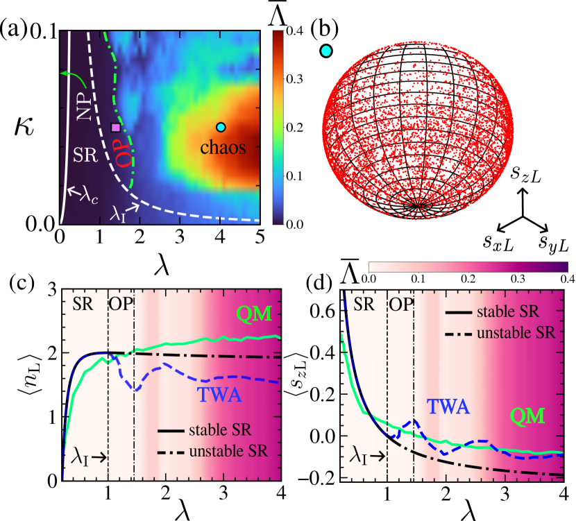
Figure 1: Dynamical phases and steady states: (a) The classical phase-diagram in $\lambda-\kappa$ plane with average Lyapunov exponent $\bar{\Lambda}$ as color scale. The NP to SR transition at $\lambda_{c}$ (solid line) and instability of SR phase at $\lambda_{\rm I}$ (dashed line) are shown. (b) The chaotic trajectory is represented by scattered points on the Bloch sphere at regular time intervals ($\lambda=4.0,\kappa=0.05$ (blue circle in (a))). Steady state: Variation of average (c) photon number $\langle n_{\rm L}\rangle$ and (d) spin polarization $\langle s_{z{\rm L}}\rangle$ of one cavitity with $\lambda$ for $\kappa=0.05$. TWA results (blue dashed line), quantum steady-state value (solid green line) and fixed point ($n^{*},s_{z}^{*}$) of SR phase are compared. The stable (unstable) SR phase is shown by black solid (dashed dotted) line. The color scales in (c,d) represent $\bar{\Lambda}$. All energies (time) are measured by $J(1/J)$. We set $\hbar,k_{B}=1$ and $\omega=2.0,\omega_{0}=0.5,\gamma_{\uparrow}=0.2,\gamma_{\downarrow}=0.1,S=2$ for all figures.

Normal phase (NP): This phase is characterized by vanishing photon number $n_{i}^{*}=0$ and spin polarization $s_{zi}^{*}=1$.

Superradiant phase (SR): At a critical coupling $\lambda_{c}$ the normal phase undergoes a continuous transition to the superradiant phase (see Fig.1(a)) with a non-vanishing photon number $n^{*}\neq 0$ and spin polarization $|s_{z}^{*}|<1$, same for each cavity. Due to the U(1) symmetry, FPs lie on a circle of radius $\sqrt{2n^{*}}$ ($\sqrt{1-(s_{z}^{*})^{2}}$) in $x-p$ ($s_{x}-s_{y}$) plane, where the dynamics always converges regardless of the initial condition. The details of this phase are given in the supplementary material [68].

Oscillatory phase (OP): Once the SR phase becomes unstable for $\lambda>\lambda_{\rm I}$ (see Fig.1(a,c,d)), the oscillatory phase emerges, where the periodic motion is identified from a single peak in the Fourier transform of trajectories [68]. Although the photon number oscillates, its phase in both cavities remains the same $\psi_{\rm L}=\psi_{\rm R}$, similar to the SR phase.

Coexistance of chaos and oscillatory dynamics: Further increasing $\lambda$ gives rise to the mixed type of dynamics, where oscillatory motion coexists with chaotic dynamics, depending on the initial conditions.

Chaotic dynamics: We also identify a regime in the phase diagram where the trajectories exhibit chaotic behavior, as depicted in Fig.1(b). To quantify the degree of chaos, we compute the mean Lyapunov exponent $\bar{\Lambda}$ [69, 70, 71] averaged over random initial phase space points, as shown in Fig.1(a).

The stable fixed point attractors, such as NP and SR phases, uniquely describe the system’s asymptotic steady state. To understand the state of the system after the instability of the SR phase, we study the semiclassical dynamics on an ensemble of phase space points using truncated Wigner approximation (TWA) [72, 73, 74]. Quantum fluctuations are incorporated by sampling initial conditions from the Husimi distribution [75] of a product of bosonic and spin coherent states, $|{\Psi_{c}}\rangle=\prod_{i}|\alpha_{i}\rangle\otimes|s_{zi},\phi_{i}\rangle$ [76] corresponding to large spin $S\gg 1$, which semiclassically represents an arbitrary phase space point $\{\alpha_{i},s_{zi}=\cos\theta_{i},\phi_{i}\}$. Importantly, we observe the emergence of a unique steady state in both oscillatory and chaotic phases, characterized by the stationary value of physical quantities such as photon number $\langle n\rangle_{\scriptscriptstyle\text{TWA}}$ and spin polarization $\langle s_{z}\rangle_{\scriptscriptstyle\text{TWA}}$ after sufficient time, which smoothly connects to the stable SR phase, as shown in Fig.1(c,d). Moreover, these dynamical variables follow stationary distribution P$(n_{i})$, P$(s_{zi})$ irrespective of initial condition (see Fig.2(a,b)). Notably, Our analysis reveals the ergodic nature of the steady state, which is based on (i) the equivalence between time and ensemble averages $\langle O\rangle_{t}=\langle O\rangle_{\scriptscriptstyle\text{TWA}}$ of dynamical quantities and (ii) their independence from initial condition [77, 78, 80, 79].

The different dynamical regimes of the steady state particularly, the onset of chaos can be revealed from the autocorrelation function,

$$C^{\scriptscriptstyle\text{TWA}}(t)=\langle O(t+\tau)O(\tau)\rangle-\langle O(t+\tau)\rangle\langle O(\tau)\rangle,$$ (4)

computed within TWA. Here, the observable $O$ is first evolved up to a long transient time $\tau$ until $\langle O(\tau)\rangle_{\scriptscriptstyle\text{TWA}}$ reaches the steady state. Although the TWA analysis indicates the formation of a steady state in the oscillatory regime, the autocorrelation function exhibits persistent oscillations, revealing its signature (see Fig.2(c)). On the contrary, in the chaotic regime, the autocorrelation function decays rapidly, as seen from Fig.2(d), confirming chaotic mixing [79, 81, 80]. Interestingly, the steady state in the oscillatory regime displays ergodicity in the absence of mixing. This contrasts with the typical closed system, where chaotic mixing leads to the ergodic steady state.

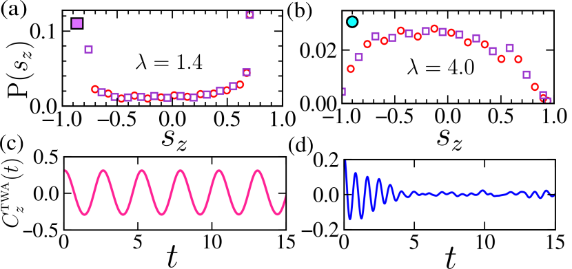
Figure 2: Comparison between oscillatory and chaotic phases: Steady-state distribution and autocorrelation function of the spin polarization $s_{z}$ of one of the cavities in the (a,c) oscillatory (OP) ($\lambda=1.4$, violet square in Fig.1(a)), (b,d) chaotic regime ($\lambda=4.0$, blue circle in Fig.1(a)). Squares and circles in (a,b) represent distributions starting from different initial conditions. We choose $\kappa=0.05$.

Quantum steady state: To this end, we investigate the properties of the quantum steady state and the signature of chaos in the presence of quantum fluctuation. We obtain the steady state density matrix (DM) $\hat{\rho}_{\rm ss}$ by solving the Master equation (see Eq.(2)) using the stochastic wavefunction approach [82, 83, 75], considering spin magnitude $S=2$.

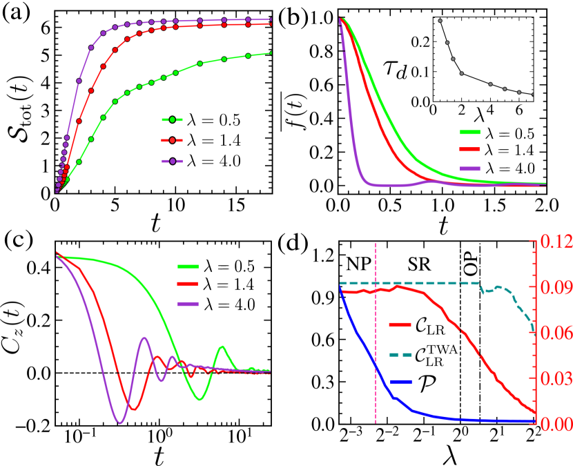
Figure 3: Quantum dynamics: (a) Evolution of total entropy $\mathcal{S}_{\rm tot}$ and (b) survival probability $\overline{f(t)}$ at different coupling $\lambda$. Inset in (b) shows variation of decay time $\tau_{d}$ of $\overline{f(t)}$ with $\lambda$. (c) Dynamics of autocorrelation of spin $C_{z}(t)$ for different $\lambda$. (d) Steady-state value of the coherence function $\mathcal{C}_{\rm LR}$ of the photon field between the cavities (solid red), corresponding TWA result (dashed greenish blue) and the purity $\mathcal{P}$ (solid blue, right axis), as a function of $\lambda$. For all figures, $\kappa=0.05$.

Similar to the classical analysis, a unique quantum steady state is formed across different dynamical regimes with increasing coupling strength. This state is characterized by the average quantities $\langle\hat{n}_{i}\rangle_{\rm ss}$ and $\langle\hat{S}_{zi}\rangle_{\rm ss}$ obtained from $\hat{\rho}_{\rm ss}$, as shown in Fig.1(c,d). For comparison with classical results, we scale these physical quantities by $S$. The steady state also exhibits ergodicity analogous to its classical counterpart, as the time average of the observables $\langle\hat{n}_{i}\rangle_{t}$ and $\langle\hat{S}_{zi}\rangle_{t}$ over a typical quantum trajectory approach to their steady-state values $\langle\hat{n}_{i}\rangle_{\rm ss}$ and $\langle\hat{S}_{zi}\rangle_{\rm ss}$ respectively [68].

Next, we study the nonequilibrium dynamics to investigate the signature of quantum mixing, as the chaotic regime is approached with increasing $\lambda$. Starting from an arbitrary initial coherent state $|{\Psi_{c}}\rangle$, representing a phase space point, we study the time evolution of survival probability $f(t)={\rm Tr}(\hat{\rho}(t)\hat{\rho}(0))$ [84, 85, 86, 87] between the initial and time-evolved density matrices. The survival probability $\overline{f(t)}$, averaged over an ensemble of initial states, decays exponentially with time and the decay rate increases as we approach the chaotic regime (see Fig.3(b)).

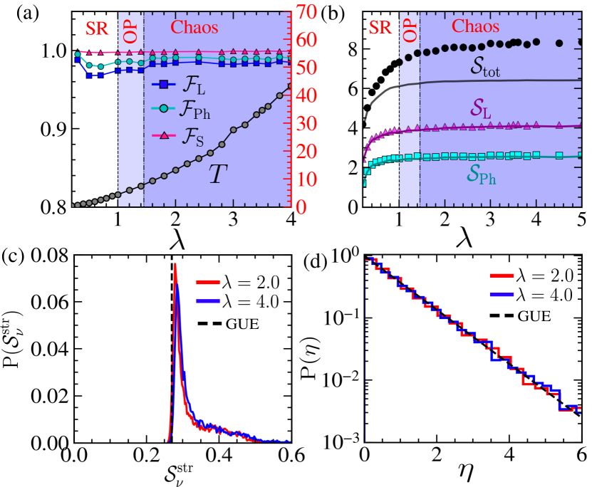
Figure 4: Subsystem thermalization: (a) Overlap between subsystem reduced DM obtained from the steady state $\hat{\rho}_{\rm ss}$ and the corresponding DM derived from the thermal state $\hat{\rho}^{\rm th}$. The overlap of the left cavity ($\mathcal{F}_{\rm L}$), photon ($\mathcal{F}_{\rm Ph}$), spin ($\mathcal{F}_{\rm S}$) of the same cavity (left axis) and effective temperature $T$ (right axis) as a function of $\lambda$. Variation of (b) total entropy $\mathcal{S}_{\rm tot}$, entanglement entropy of the left cavity $\mathcal{S}_{\rm L}$ and photon field of that cavity $\mathcal{S}_{\rm Ph}$ in the steady state $\hat{\rho}_{\rm ss}$ with $\lambda$. The solid lines (markers) represent the entropies obtained from $\hat{\rho}_{\rm ss}$ ($\hat{\rho}^{\rm th}$). Classical phases are marked by blue colored regimes. Statistics of $\hat{\rho}_{\rm ss}$: (c) distribution of structural entropy $\mathcal{S}_{\nu}^{\rm str}$ of eigenstates of $\hat{\rho}_{\rm ss}$ in the chaotic regime. Black dashed line represents the corresponding GUE value. (d) Distribution of elements $\eta=|\Psi_{\nu}^{j}|^{2}N_{\rm dim}$ of typical eigenstate of steady state at different $\lambda$. Black dashed line represents the corresponding GUE distribution. Parameter chosen: $\kappa=0.05$.

From the time evolved density matrix, we also obtain the total entropy $\mathcal{S}_{\rm tot}=-{\rm Tr}(\hat{\rho}(t)\ln\hat{\rho}(t))$, which grows linearly and attains a saturation value corresponding to the steady state. As evident from Fig.3(a), both the growth rate and the saturation value of $\mathcal{S}_{\rm tot}$ increases with $\lambda$. Also, the reduced density matrix $\hat{\rho}_{A}={\rm Tr}_{\bar{A}}(\hat{\rho})$ of subsystem $A$ can be obtained by tracing out the remaining degrees of freedom $\bar{A}$, which in turn yields the corresponding entanglement entropy (EE) $\mathcal{S}_{A}=-{\rm Tr}(\hat{\rho}_{A}\ln\hat{\rho}_{A})$. Additionally, the EE corresponding to one of the cavities $\mathcal{S}_{\rm L}$ exhibits similar behavior [68]. Such linear growth in EE is typically observed as a signature of chaos in isolated quantum systems [4, 6, 88, 89, 90, 91]. The underlying chaos can also be unveiled from the individual quantum trajectories, which show a spreading of the power spectrum over a wide range of frequencies [68, 92].

We also analyze the autocorrelation function corresponding to the steady state $C(t)=\langle O(t)O(0)\rangle-\langle O(t)\rangle\langle O(0)\rangle$, following the prescription of stochastic wave-function [93, 83]. As seen from Fig.3(c), the autocorrelation function $C_{z}(t)$ of the spin in one cavity vanishes rapidly and the decay time decreases with increasing coupling strength $\lambda$. Such fast decay of $C_{z}(t)$ signifies enhanced mixing dynamics due to the onset of chaos.

In addition, the quantum fluctuations enhance the decay rate of $C_{z}(t)$ as compared to the classical counterpart. Importantly, the oscillatory phase is washed out due to the strong quantum fluctuation, which is evident from the decaying autocorrelation function (see Fig.3(c)). Furthermore, the combined effect of quantum fluctuations and chaotic mixing suppresses the purity of the steady state $\mathcal{P}={\rm Tr}(\hat{\rho}_{\rm ss}^{2})$ significantly, even in the superradiant phase, as depicted in Fig.3(d). The coherence of the photon fields between the two cavities in the steady state can be quantified from,

$$\mathcal{C}_{\rm LR}=\frac{\langle\hat{a}_{\rm L}^{\dagger}\hat{a}_{\rm R}+\hat{a}_{\rm R}^{\dagger}\hat{a}_{L}\rangle}{2\sqrt{\langle\hat{n}_{\rm L}\rangle\langle\hat{n}_{\rm R}\rangle}},$$ (5)

which classically reduces to $\mathcal{C}_{\rm LR}^{\rm TWA}=\langle\cos(\psi_{\rm L}-\psi_{\rm R})\rangle_{\scriptscriptstyle\text{TWA}}$. In the superradiant and oscillatory phase, $\mathcal{C}_{\rm LR}^{\rm TWA}$ attains the value unity and decays in the chaotic regime, as observed from the TWA analysis. Similar behavior can also be observed quantum mechanically, however, the decay starts even before the instability of SR phase, as a result of quantum fluctuations (see Fig.3(d)). It is clear from this analysis that the mixing dynamics due to the underlying chaos as well as quantum fluctuation can lead to the destruction of the coherence of the system, which can be probed from the state of the photon field of the respective cavities. The semiclassical distribution of the photon field for the sufficiently small value of $\lambda$ in the stable SR phase is peaked around the circle of the classical fixed points of radius $\sqrt{2n^{*}}$. As we approach the chaotic regime, this distribution spreads and peaks around the center, resembling a thermal distribution [68]. Such an observation suggests chaos-induced thermalization in this dissipative system, which we discuss next.

Subsystem thermalization: To investigate thermalization of this open system, we consider the thermal density matrix of TCD $\hat{\rho}^{\rm th}=\exp(-\beta(\hat{\mathcal{H}}-\mu\hat{\mathcal{N}}))/Z$ with $Z$ being the partition function. The inverse temperature $\beta$ and the chemical potential $\mu$ are uniquely determined from the mean energy $\langle\hat{\mathcal{H}}\rangle$ and the average number of excitations $\langle\hat{\mathcal{N}}\rangle$ obtained from the steady-state density matrix $\hat{\rho}_{\rm ss}$. Clearly, $\hat{\rho}^{\rm th}$ does not correspond to the steady state of the Master equation (Eq.(2)) in the presence of dissipation. However, the state of the subsystem $A$ can be well described by the reduced DM $\hat{\rho}_{A}^{\rm th}$ derived from the thermal state $\hat{\rho}^{\rm th}$ of the full system. We compare the reduced DMs $\hat{\rho}_{A}^{\rm ss}$ and $\hat{\rho}_{A}^{\rm th}$ obtained from the steady state and thermal DM respectively, using their overlap $\mathcal{F}_{A}={\rm Tr}\sqrt{\sqrt{\hat{\rho}_{A}^{\rm ss}}\hat{\rho}_{A}^{\rm th}\sqrt{\hat{\rho}_{A}^{\rm ss}}}$ [84, 85]. Considering one of the cavities as well as its photonic and spin sector as subsystems, we compute $\mathcal{F}_{A}$, which remains close to unity, as evident from Fig.4(a). Moreover, trace-distances between $\hat{\rho}_{A}^{\rm ss}$ and $\hat{\rho}_{A}^{\rm th}$ remain small [68], indicating the similarity between them. Consequently, the entanglement entropies of the corresponding subsystems (see Fig.4(b)) as well as the average values of the observables such as $\langle\hat{n}_{i}\rangle$ and $\langle\hat{S}_{zi}\rangle$ exhibit agreement with those of the thermal state [68], confirming the validity of subsystem thermalization [94, 95, 96] in open TCD over a range of $\lambda$. Surprisingly, the steady state follows the subsystem thermalization over a large range of coupling strength even outside the chaotic regime, however, the effective temperature $T$ increases with the degree of chaos, as shown in Fig.4(a).

For a deeper understanding of this scenario, we also study the statistics of eigenstates $|{\Psi_{\nu}}\rangle$ of the steady-state DM $\hat{\rho}_{\rm ss}$. We compute the structural entropy [97, 98] of $|{\Psi_{\nu}}\rangle$,

$$\mathcal{S}_{\nu}^{\rm str}=-\sum_{j}|\Psi_{\nu}^{j}|^{2}\ln(|\Psi_{\nu}^{j}|^{2})+\ln\left(\sum_{j}|\Psi_{\nu}^{j}|^{4}\right),$$ (6)

and study its distribution, which is sharply peaked around a value $\mathcal{S}^{\rm str}\approx 0.27$ (see Fig.4(c)) corresponding to the Gaussian unitary ensemble (GUE) class of the random matrix theory (RMT) [3, 99]. Moreover, the elements $\eta=|\Psi_{\nu}^{j}|^{2}N_{\rm dim}$ of the eigenstate $|{\Psi_{\nu}}\rangle$ (with dimension $N_{\rm dim}$), follows the GUE distribution ${\rm P}(\eta)=\exp(-\eta)$ [1], as seen from Fig.4(d), indicating the chaotic nature of such states. The steady state of a random Liouvillian also follows the GUE distribution [22, 100], however in the present case, we do not find any signature of level repulsion in the Liouvillian spectrum, which on the contrary resembles to 2d-Poisson distribution, even in the chaotic regime [68].

Discussion: Our study unveils the emergence of a steady state with intriguing properties, especially the onset of chaos in an open atom-photon dimer system. The appropriate classical limit of this system enables us to explore the classical-quantum correspondence of dissipative chaos, which is absent in a generic quantum system. The rapid decay of the correlation function and survival probability, along with the growth of entropy, manifest the chaotic mixing of the emergent steady state, which serves as a more tangible signature of dissipative chaos compared to spectral statistics. Both chaos and quantum fluctuations result in the loss of coherence, leading to the formation of an incoherent photonic fluid, which can be probed experimentally. Remarkably, this steady state follows thermalization of the subsystems, revealing its connection with the random matrix.

In conclusion, this atom-photon dimer system exhibits intriguing nonequilibrium phenomena and sheds light on dissipative quantum chaos, with results readily testable in current cavity and circuit QED setups.

Acknowledgments: We thank Krishnendu Sengupta and Sudip Sinha for comments and fruitful discussions. D.M. acknowledges support from Prime Minister Research Fellowship (PMRF).

References

- [1] F. Haake, Quantum Signatures of Chaos, Springer Science and Business Media (Springer, Berlin, Heidelberg, 2013), Vol. 54.
- [2] O. Bohigas, M. J. Giannoni, and C. Schmit, Phys. Rev. Lett. 52, 1 (1984).
- [3] F. M. Izrailev, Phys. Rep. 196, 299 (1990);
- [4] L. D’Alessio, Y. Kafri, A. Polkovnikov, and M. Rigol, Adv. Phys. 65, 239 (2016).
- [5] M. Ueda, Nat. Rev. Phys. 2, 669 (2020).
- [6] F. Borgonovi, F. M. Izrailev, L. F. Santos, and V. G. Zelevinsky, Phys. Rep. 626, 1 (2016).
- [7] M. Rigol, V. Dunjko, M. Olshanii, Nature 452, 854 (2008).
- [8] J. M. Deutsch, Phys. Rev. A 43, 2046 (1991).
- [9] M. Srednicki, Phys. Rev. E 50, 888 (1994).
- [10] R. Grobe, F. Haake, and Hans-Jürgen Sommers, Phys. Rev. Lett. 61, 1899 (1988); R. Grobe and F. Haake, Phys. Rev. Lett. 62, 2893–2896 (1989).
- [11] G. G. Carlo, G. Benenti, and D. L. Shepelyansky, Phys. Rev. Lett. 95, 164101 (2005).
- [12] G. G. Carlo, G. Benenti, G. Casati, and D. L. Shepelyansky, Phys. Rev. Lett. 94, 164101 (2005).
- [13] D. Dahan, G. Arwas, and E. Grosfeld, npj Quantum Inf 8, 14 (2022).
- [14] D. Mondal, K. Sengupta, S. Sinha, arXiv:2310.12779 (2023).
- [15] G. Vivek, D. Mondal, S. Chakraborty, S. Sinha, arXiv:2405.13809 (2024).
- [16] F. Ferrari, L. Gravina, D. Eeltink, P. Scarlino, V. Savona, F. Minganti, arXiv.2305.15479 (2023).
- [17] M. Žnidarič, T. Prosen, G. Benenti, G. Casati, and D. Rossini, Phys. Rev. E 81, 051135 (2010).
- [18] I. Reichental, A. Klempner, Y. Kafri, and D. Podolsky, Phys. Rev. B 97, 134301 (2018).
- [19] T. Shirai and T. Mori, Phys. Rev. E 101, 042116 (2020).
- [20] F. Vicentini, A. Biella, N. Regnault, and C. Ciuti, Phys. Rev. Lett. 122, 250503 (2019).
- [21] L. Sá, P. Ribeiro, and T. Prosen, Phys. Rev. X 10, 021019 (2020).
- [22] L. Sá, P. Ribeiro, and T. Prosen, J. Phys. A: Math. Theor. 53 305303 (2020).
- [23] S. Denisov, T. Laptyeva, W. Tarnowski, D. Chruściński, and K. Życzkowski, Phys. Rev. Lett. 123, 140403 (2019).
- [24] M. Prasad, H. K. Yadalam, C. Aron, and M. Kulkarni, Phys. Rev. A 105, L050201 (2022).
- [25] D. Villaseǹor, L. F. Santos, P. Barberis-Blostein, arXiv:2406.07616 (2024).
- [26] C. Emary and T. Brandes, Phys. Rev. Lett. 90, 044101 (2003);
- [27] A. Altland and F. Haake, Phys. Rev. Lett. 108, 073601 (2012); New J. Phys. 14, 073011 (2012).
- [28] D. Villaseñor, S. Pilatowsky-Cameo, M. A. Bastarrachea-Magnani, S. Lerma-Hernández, L. F. Santos, and J. G. Hirsch, Entropy 25, 8 (2022).
- [29] T. Dittrich, R. Graham, Europhys. Lett. 7, 287 (1988).
- [30] P.S.Muraev, D.N.Maksimov, and A.R.Kolovsky, Entropy 2023, 25, 117.
- [31] A. R. Kolovsky, Phys. Rev. E 106, 014209 (2022).
- [32] S. Sinha, S. Ray and S. Sinha, J. Phys.: Condens. Matter 36 163001 (2024).
- [33] F. Mivehvar, F. Piazza, T. Donner, H. Ritsch, Adv. Phys. 70, 1–153 (2021).
- [34] H. Ritsch, P. Domokos, F. Brennecke, and T. Esslinger, Rev. Mod. Phys. 85, 553 (2013).
- [35] M. Müller, S. Diehl, G. Pupillo, and P. Zoller, Adv. At. Mol. Opt. Phys. 61, 1 (2012).
- [36] F. Damanet, E. Mascarenhas, D. Pekker, and A. J. Daley, Phys. Rev. Lett. 123, 180402 (2019).
- [37] P.M. Harrington, E.J. Mueller, and K.W. Murch, Nat Rev Phys 4, 660–671 (2022).
- [38] R. Lin, R. Rosa-Medina, F. Ferri, F. Finger, K. Kroeger, T. Donner, T. Esslinger, and R. Chitra, Phys. Rev. Lett. 128, 153601 (2022).
- [39] H. Weimer, A. Kshetrimayum, and R. Orús, Rev. Mod. Phys. 93, 015008 (2021).
- [40] F. Damanet, A. J. Daley, and J. Keeling, Phys. Rev. A 99, 033845 (2019).
- [41] J. Klinder, H. Keßler, M. Wolke, L. Mathey, and A. Hemmerich, Proc. Natl. Acad. Sci. U.S.A. 112, 3290 (2015).
- [42] S. Diehl, A. Tomadin, A. Micheli, R. Fazio, and P. Zoller, Phys. Rev. Lett. 105, 015702 (2010).
- [43] H. J. Carmichael, Phys. Rev. X 5, 031028 (2015).
- [44] K. C. Stitely, A. Giraldo, B. Krauskopf, and S. Parkins, Phys. Rev. Research 2, 033131 (2020).
- [45] K. C. Stitely, A. Giraldo, B Krauskopf, and S. Parkins, Phys. Rev. Research 4, 023101 (2022).
- [46] K. C. Stitely, S. J. Masson, A. Giraldo, B. Krauskopf, and S. Parkins, Phys. Rev. A 102, 063702 (2020).
- [47] C. J. Zhu, L. L. Ping, Y. P. Yang, and G. S. Agarwal, Phys. Rev. Lett. 124, 073602 (2020).
- [48] S. Ray, A. Vardi, and D. Cohen, Phys. Rev. Lett. 128, 130604 (2022).
- [49] K. C. Stitely, F. Finger, R. Rosa-Medina, F. Ferri, T. Donner, T. Esslinger, S. Parkins, and B. Krauskopf, Phys. Rev. Lett. 131, 143604 (2023).
- [50] J. Li, R. Fazio, and S. Chesi, New J. Phys. 24, 083039 (2022).
- [51] W. Kopylov, M. Radonjić, T. Brandes, A. Balaž, and A. Pelster, Phys. Rev. A 92, 063832 (2015).
- [52] F. Carollo and I. Lesanovsky, Phys. Rev. Lett. 126, 230601 (2021).
- [53] J. M. Raimond, M. Brune, and S. Haroche, Rev. Mod. Phys. 73, 565 (2001).
- [54] A. Blais, A. L. Grimsmo, S. M. Girvin, and A. Wallraff, Rev. Mod. Phys. 93, 025005 (2021).
- [55] J. Léonard, A. Morales, P. Zupancic, T. Esslinger, and T. Donner, Nature (London) 543, 87 (2017).
- [56] J. Léonard, A. Morales, P. Zupancic, T. Donner, and T. Esslinger, Science 358, 1415 (2017).
- [57] J.A. Muniz, D. Barberena, R.J. Lewis-Swan, D. J. Young, J. R. K. Cline, A. M. Rey, Nature 580, 602–607 (2020).
- [58] D.J. Young, A. Chu, E.Y.Song, D. Barberena, D. Wellnitz, Z. Niu, V. M. Schäfer, R. J. Lewis-Swan, A. M. Rey and J. K. Thompson, Nature 625, 679–684 (2024).
- [59] F. Letscher, O. Thomas, T. Niederprüm, M. Fleischhauer, and H. Ott, Phys. Rev. X 7, 021020 (2017).
- [60] R. M. Kroeze, Y. Guo, V. D. Vaidya, J. Keeling, and B. L. Lev, Phys. Rev. Lett. 121, 163601 (2018).
- [61] M. Fitzpatrick, N. M. Sundaresan, A. C. Y. Li, J. Koch and A. A. Houck, Phys. Rev. X 7, 011016 (2017).
- [62] M. Tavis and F. W. Cummings, Phys. Rev. 170, 379 (1968).
- [63] H-P Eckle, Models of Quantum Matter: A First Course on Integrability and the Bethe Ansatz, Chap 12, 474 (Oxford University Press, (2021)).
- [64] V. Gorini, A. Kossakowski, and E. C. G. Sudarshan, J. Math. Phys. (N.Y.) 17, 821–825 (1976).
- [65] G. Lindblad, Commun. Math. Phys. 48, 119–130 (1976).
- [66] H. P. Breuer and F. Petruccione, The Theory of Open Quantum Systems (Oxford University Press, Oxford, 2007).
- [67] L. da Silva Souza, L. F. dos Prazeres, and F. Iemini, Phys. Rev. Lett. 130, 180401 (2023).
- [68] See the Supplementary material for the details of the classical dynamical phases, quantum ergodicity, subsystem thermalization and statistics of the Liouvillian spectrum in the present model.
- [69] S. H. Strogatz, Nonlinear Dynamics and Chaos (Westview Press, Boulder, CO, 2007).
- [70] A. J. Lichtenberg and M. A. Lieberman, Regular and chaotic dynamics, (Springer-Verlag,1992).
- [71] J. Chávez-Carlos, M. A. Bastarrachea-Magnani, S. Lerma-Hernández, and J. G. Hirsch, Phys. Rev. E 94, 022209 (2016).
- [72] P. B. Blakie, A. S. Bradley, M. J. Davis, R. J. Ballagh, and C. W. Gardiner, Adv. Phys. 57, 363 (2008).
- [73] A. Polkovnikov, Ann. Phys. 325, 1790 (2010).
- [74] J. Schachenmayer, A. Pikovsky, and A. M. Rey, Phys. Rev. X 5, 011022 (2015).
- [75] C. Gardiner and P. Zoller, Quantum Noise: A Handbook of Markovian and Non-Markovian Quantum Stochastic Methods with Applications to Quantum Optics (Springer Science, New York, 2004).
- [76] J. M. Radcliffe, J. Phys. A: Gen.Phys., 4, 313 (1971).
- [77] I. P. Cornfield, S. V. Fomin, and Y. G. Sinai, 1982 Ergodic Theory (Springer) .
- [78] P. R. Halmos 2017 Lectures on Ergodic Theory (Dover).
- [79] R. Frigg, J. Berkovitz, and F. Kronz, The Ergodic Hierarchy, in The Stanford Encyclopedia of Philosophy, (Fall 2020 Edition), edited by E. N. Zalta, https://plato.stanford.edu/archives/ fall2020/entries/ergodic-hierarchy/.
- [80] E. Ott, Chaos in dynamical systems (1993, Cambridge University Press).
- [81] D. Ruelle, Chaotic evolution and strange attractors (1989, Cambridge University Press).
- [82] H. Carmichael, An Open Systems Approach to Quantum Optics. Springer-Verlag (1993).
- [83] K. Mølmer, Y. Castin and J. Dalibard, J. Opt. Soc. Am. B 10, 524 (1993).
- [84] M. A. Nielsen and I. L. Chuang, Quantum Computation and Quantum Information, (Cambridge University Press, Cambridge, England, 2000).
- [85] H. Nha and H. J. Carmichael, Phys. Rev. A 71, 032336 (2005).
- [86] F. Tonielli, R. Fazio, S. Diehl, and J. Marino, Phys. Rev. Lett. 122, 040604 (2019).
- [87] For unitary dynamics of initial pure state , the quantity reduces to the usual definition of survival probability . Additionally, it is related with the more general definition of overlap between two mixed density matrices (see Ref. [84, 85]).
- [88] A. Piga, M. Lewenstein, and J. Q. Quach, Phys. Rev. E 99 032213 (2019).
- [89] X. Wang, S. Ghose, B. C. Sanders, and B. Hu, Phys. Rev. E 70 016217 (2004).
- [90] H. Fujisaki, T. Miyadera, and A. Tanaka, Phys. Rev. E 67, 066201 (2003).
- [91] S. Ray, A. Ghosh, and S. Sinha, Phys. Rev. E 94, 032103 (2016).
- [92] T. Geisel, Phys. Rev. A 41, 2989 (1990); Erratum Phys. Rev. A 42, 7491 (1990).
- [93] S. Wolff, A. Sheikhan, C. Kollath, SciPost Phys. Core 3, 010 (2020)
- [94] A. Dymarsky, N. Lashkari, and H. Liu, Phys. Rev. E 97, 012140 (2018);
- [95] Z. Huang and Xiao-Kan Guo, Phys. Rev. E 109, 054120 (2024).
- [96] J. R. Garrison and T. Grover, Phys. Rev. X 8, 021026 (2018).
- [97] J. Pipek and I. Varga, Phys. Rev. A 46, 3148 (1992).
- [98] P. Jacquod and I. Varga, Phys. Rev. Lett. 89, 134101 (2002).
- [99] S. Ray, B. Mukherjee, S. Sinha, and K. Sengupta, Phys. Rev. A 96, 023607 (2017).
- [100] T. Prosen and M. Žnidarič, Phys. Rev. Lett. 111, 124101 (2013).