Structured and Balanced Multi-component
and Multi-layer Networks

Structured and Balanced Multi-component
and Multi-layer Neural Networks

Abstract

In this work, we propose a balanced multi-component and multi-layer neural network (MMNN) structure to approximate functions with complex features with both accuracy and efficiency in terms of degrees of freedom and computation cost. The main idea is motivated by a multi-component, each of which can be approximated effectively by a single-layer network, and multi-layer decomposition in a “divide-and-conquer” type of strategy to deal with a complex function. While an easy modification to fully connected neural networks (FCNNs) or multi-layer perceptrons (MLPs) through the introduction of balanced multi-component structures in the network, MMNNs achieve a significant reduction of training parameters, a much more efficient training process, and a much improved accuracy compared to FCNNs or MLPs. Extensive numerical experiments are presented to illustrate the effectiveness of MMNNs in approximating high oscillatory functions and its automatic adaptivity in capturing localized features. Our codes and implementation details are available here.

Key words. deep neural networks, rectified linear unit, function compositions, Fourier series

1 Introduction

The key use of neural networks is to approximate an input-to-output relation, i.e., a mapping or a function in the mathematics term. In this work, we continue our study of numerical understanding of neural network approximation of functions from representation to learning dynamics. In our earlier study [38], we demonstrated that a one-hidden-layer (also known as a two-layer or shallow) network is essentially a “low-pass filter” when approximating a function in practice. Due to the strong correlation among the family of activation functions (parameterized by the weight and bias), such as $\mathtt{ReLU}$  (rectified linear unit), the Gram matrix, the element of which is the pairwise correlation (inner product) of the activation functions, has a fast spectral decay. If initialized randomly, the eigenvectors of the Gram matrix correspond to generalized Fourier modes from low frequency to high frequency ordered corresponding to decreasing eigenvalues. Due to the ill-conditioning of the representation, no matter how wide a one-hidden-layer network is, it can only learn and approximate smooth functions or sample low-frequency modes effectively and stably (with respect to noise or machine round-off errors).

In this work, we propose a balanced multi-component and multi-layer neural network (MMNN) structure based on our previous understanding of a one-hidden-layer network. First, we show that a multi-layer network with a multi-component structure, each of which can be approximated well and effectively by a one-hidden-layer network, can overcome the limitation of a shallow network by smooth decomposition and transformation. Compared to a fully connected neural network of a similar structure, our proposed MMNN is much more effective in terms of representation, training, and accuracy in approximating functions, especially for functions containing complex features, e.g., high-frequency modes. The key idea of MMNNs is to view a linear combination of activation functions as randomly parameterized basis functions, called a component, as a whole to represent a smooth function. Each layer has multiple components all sharing the common basis functions with different linear combinations. The number of components, called rank, is typically much smaller than the layer’s width and increases to enhance the flexibility of decomposition when dealing with more complex functions. These components are combined and composed (through layers) in a structured and balanced way in terms of network width, rank, and depth to approximate a complicated function effectively. Another important feature we used in practice is that weights and biases inside each activation function are randomly assigned and fixed during the optimization while the linear combination weights of activation functions in each component are trained. This leads to more efficient training processes motivated by our finding that a one-hidden-layer neural network can be trained effectively to approximate a smooth function well using random basis functions. We also demonstrate interesting learning dynamics based on Adam optimizer [14], which is crucial for the successful and efficient training of MMNNs. An important remark is that a balanced and holistic approach needs to consider both representation and optimization as well as their interplay altogether.

The outline of this paper is summarized as follows. In Section 2, the design of MMNNs is proposed and explained. Then, in Section 3, a mathematical framework for smooth decomposition and transformation using the MMNN architecture is presented, demonstrating that each component can be effectively approximated by a one-hidden-layer network. Extensive numerical experiments are presented in Section 4 to verify the analysis and demonstrate the effectiveness of MMNNs in the approximation of more complicated functions. Further discussion is presented in Section 5, where more insights and implementation guidelines of MMNNs are provided. Finally, remarks and conclusions are provided in Section 6.

2 Multi-component and multi-layer neural network (MMNN)

This section begins with an overview of the main notations used in this paper, as detailed in Section 2.1. Subsequently, we introduce a novel network architecture, the Multi-component and Multi-layer Neural Network (MMNN), which is developed based on the balanced decomposition principle discussed in Section 2.2. Following this, in Section 2.3, we outline the learning strategy of MMNN and highlight its advantages over other methods. Finally, in Section 2.4, we compare the numerical performance of MMNNs and FCNNs.

2.1 Notations

The following is an overview of the basic notations used in this paper.

• The symbols ${\mathbb{N}}$, ${\mathbb{Z}}$, ${\mathbb{Q}}$, and ${\mathbb{R}}$ are used to denote the sets of natural numbers (including $0$), integers, rational numbers, and real numbers, respectively. The set of positive natural numbers is denoted as ${\mathbb{N}}^{+}={\mathbb{N}}\backslash\{0\}$.

• The indicator (or characteristic) function of a set $A$, denoted by ${\mathds{1}}_{A}$, is a function that takes the value $1$ for elements of $A$ and $0$ for elements not in $A$.

• The floor and ceiling functions of a real number $x$ can be represented as $\lfloor x\rfloor=\max\{n:n\leq x,\ n\in{\mathbb{Z}}\}$ and $\lceil x\rceil=\min\{n:n\geq x,\ n\in{\mathbb{Z}}\}$.

• Vectors are denoted by bold lowercase letters, such as ${\bm{a}}=(a_{1},\mathinner{\mkern-0.1mu\cdotp\mkern-0.3mu\cdotp\mkern-0.3mu\cdotp\mkern-0.1mu},a_{n})\in{\mathbb{R}}^{n}$. On the other hand, matrices are represented by bold uppercase letters. For example, $\bm{A}\in\mathbb{R}^{m\times n}$ refers to a real matrix of size $m\times n$, and $\bm{A}^{\textsf{T}}$ denotes the transpose of matrix $\bm{A}$.

• Slicing notation is used for a vector ${\bm{x}}=(x_{1},\mathinner{\mkern-0.1mu\cdotp\mkern-0.3mu\cdotp\mkern-0.3mu\cdotp\mkern-0.1mu},x_{d})\in{\mathbb{R}}^{d}$, where ${\bm{x}}{[n:m]}$ denotes a slice of ${\bm{x}}$ from its $n$-th to the $m$-th entries for any $n,m\in\{1,2,\mathinner{\mkern-0.1mu\cdotp\mkern-0.3mu\cdotp\mkern-0.3mu\cdotp\mkern-0.1mu},d\}$ with $n\leq m$ and ${\bm{x}}{[n]}$ denotes the $n$-th entry of ${\bm{x}}$. For example, if ${\bm{x}}=(x_{1},x_{2},x_{3})\in{\mathbb{R}}^{3}$, then $(5{\bm{x}}){[2:3]}=(5x_{2},5x_{3})$ and $(6{\bm{x}}+1){[3]}=6x_{3}+1$. A similar notation is employed for matrices. For instance, ${\bm{A}}[:,i]$ refers to the $i$-th column of ${\bm{A}}$, whereas ${\bm{A}}[i,:]$ indicates the $i$-th row of ${\bm{A}}$. Additionally, ${\bm{A}}[i,n:m]$ corresponds to $({\bm{A}}[i,:])[n:m]$, which means it extracts the entries from the $n$-th to the $m$-th in the $i$-th row.

2.2 Architecture of MMNNs

In this section, we introduce our Multi-component and Multi-layer Neural Network (MMNN). Each layer of MMNN is a (shallow) neural network of the form

$${\bm{h}}({\bm{x}})={\bm{A}}\sigma({\bm{W}}{\bm{x}}+{\bm{b}})+{\bm{c}}$$

to approximate a vector-valued function ${\bm{f}}\in C([0,1]^{d_{\textnormal{in}}};{\mathbb{R}}^{d_{\textnormal{out}}})$, where ${\bm{W}}\in{\mathbb{R}}^{n\times{d_{\textnormal{in}}}},{\bm{A}}\in{\mathbb{R}}^{{d_{\textnormal{out}}}\times n}$, and $n$ is the width of this network. Here, $\sigma:\mathbb{R}\to\mathbb{R}$ represents the activation function that can be applied elementwise to vector inputs. Throughout this paper, the activation function is $\mathtt{ReLU}$, unless otherwise specified. One can also write it in a more compact form,

$${\bm{h}}={\bm{A}}\sigma({\bm{W}}{\bm{x}}+{\bm{b}})+{\bm{c}}={\widetilde{\bm{A}}}\left[\begin{matrix}\sigma({\widetilde{\bm{W}}}{\widetilde{\bm{x}}})\\ 1\end{matrix}\right]={\widetilde{\bm{A}}}\sigma({\widetilde{\bm{W}}}{\widetilde{\bm{x}}}),$$ (1)

where

$${\widetilde{\bm{W}}}=\left[\begin{matrix}{\bm{W}},{\bm{b}}\end{matrix}\right],\quad{\widetilde{\bm{A}}}=\left[\begin{matrix}{\bm{A}},{\bm{c}}\end{matrix}\right],\quad{\widetilde{\bm{x}}}=\left[\begin{matrix}{\bm{x}}\\ 1\end{matrix}\right].$$

We call each element of ${\bm{h}}$, i.e., ${\bm{h}}{[i]}=\widetilde{\bm{A}}{[i,:]}\cdot\left[\begin{matrix}\sigma({\widetilde{\bm{W}}}{\widetilde{\bm{x}}})\\ 1\end{matrix}\right]$ for $i=1,2,\mathinner{\mkern-0.1mu\cdotp\mkern-0.3mu\cdotp\mkern-0.3mu\cdotp\mkern-0.1mu},d_{out}$, a component. Here are a few key features of ${\bm{h}}$:

1. Each component is viewed as a linear combination of basis functions $\sigma({\bm{W}}{[i,:]}\cdot{\bm{x}}+{\bm{b}}[i]),\,i=1,2,\mathinner{\mkern-0.1mu\cdotp\mkern-0.3mu\cdotp\mkern-0.3mu\cdotp\mkern-0.1mu},n$, which is a function in ${\bm{x}}$, as a whole.

2. Different components of ${\bm{h}}$ share the same set of basis with different coefficients $\widetilde{\bm{A}}[i,:]$.

3. Only ${\widetilde{\bm{A}}}$ are trained while ${\widetilde{\bm{W}}}$ are randomly assigned and fixed.

4. The output dimension ${d_{\textnormal{out}}}$ and network width $n$ can be tuned according to the intrinsic dimension and complexity of the problem.

In comparison, each layer in a typical deep FCNN takes the form $\sigma({\widetilde{\bm{W}}}{\widetilde{\bm{x}}})$, and each hidden neuron is individually a function of the input ${\bm{x}}$ or each point ${\bm{x}}\in{\mathbb{R}}^{d_{in}}$ is mapped to ${\mathbb{R}}^{n}$, where $n$ is the layer width. All weights ${\widetilde{\bm{W}}}$ are training parameters. In MMNN, each layer is composed of multiple components ${\widetilde{\bm{A}}}\sigma({\widetilde{\bm{W}}}{\widetilde{\bm{x}}})$. Each component is a linear combination of randomly parameterized hidden neurons $\sigma({\widetilde{\bm{W}}}{\widetilde{\bm{x}}})$, which can be more effectively and stably trained through ${\widetilde{\bm{A}}}$ as a smooth decomposition/transformation. Typically the number of components $d_{out}$ is (much) smaller than the layer width $n$ in our experiments.

A MMNN is a multi-layer composition of ${\bm{h}}_{i}$, i.e., ${\bm{h}}:{\mathbb{R}}^{d_{\textnormal{in}}}\mapsto{\mathbb{R}}^{d_{\textnormal{out}}}$

$${\bm{h}}={\bm{h}}_{m}\circ\mathinner{\mkern-0.1mu\cdotp\mkern-0.3mu\cdotp\mkern-0.3mu\cdotp\mkern-0.1mu}\circ{\bm{h}}_{2}\circ{\bm{h}}_{1},$$

where each ${\bm{h}}_{i}:{\mathbb{R}}^{d_{i-1}}\mapsto{\mathbb{R}}^{d_{i}}$ is a multi-component shallow network defined in (1) of width $n_{i}$, where

$$d_{0}={d_{\textnormal{in}}},\qquad d_{1},\mathinner{\mkern-0.1mu\cdotp\mkern-0.3mu\cdotp\mkern-0.3mu\cdotp\mkern-0.1mu},d_{m-1}\ll n_{i},\qquad d_{m}={d_{\textnormal{out}}}.$$

The width of this MMNN is defined as $\max\{n_{i}:i=1,2,\mathinner{\mkern-0.1mu\cdotp\mkern-0.3mu\cdotp\mkern-0.3mu\cdotp\mkern-0.1mu},m-1\}$, the rank as $\max\{d_{i}:i=1,2,\mathinner{\mkern-0.1mu\cdotp\mkern-0.3mu\cdotp\mkern-0.3mu\cdotp\mkern-0.1mu},m-1\}$, and the depth as $m$. To simplify, we denote a network with width $w$, rank $r$, and depth $l$ using the compact notation $(w,r,l)$. See Figure 1(a) for an illustration of MMNN of size $(4,2,2)$. In contrast, an FCNN ${\bm{\phi}}$ can be expressed in the following composition form

$${\bm{\phi}}={\bm{\mathcal{L}}}_{L}\circ\sigma\circ{\bm{\mathcal{L}}}_{L-1}\circ\ \mathinner{\mkern-0.1mu\cdotp\mkern-0.3mu\cdotp\mkern-0.3mu\cdotp\mkern-0.1mu}\ \circ\sigma\circ{\bm{\mathcal{L}}}_{1}\circ\sigma\circ{\bm{\mathcal{L}}}_{0},$$

where ${\bm{\mathcal{L}}}_{i}$ is an affine linear map given by ${\bm{\mathcal{L}}}_{i}({\bm{y}})={\bm{W}}_{i}\cdot{\bm{y}}+{\bm{b}}_{i}$. Readers are referred to Figure 1(b) for an illustration and also a comparison with the MMNN.

For very deep MMNNs, one can borrow ideas from ResNets [8] to address the gradient vanishing issue, making training more efficient. Incorporating this idea, we propose a new architecture given by a multi-layer composition of ${\bm{I}}+{\bm{h}}_{i}$, i.e., ${\bm{h}}:{\mathbb{R}}^{d_{\textnormal{in}}}\mapsto{\mathbb{R}}^{d_{\textnormal{out}}}$

$${\bm{h}}={\bm{h}}_{m}\circ({\bm{I}}+{\bm{h}}_{m-1})\circ\mathinner{\mkern-0.1mu\cdotp\mkern-0.3mu\cdotp\mkern-0.3mu\cdotp\mkern-0.1mu}\circ({\bm{I}}+{\bm{h}}_{3})\circ({\bm{I}}+{\bm{h}}_{2})\circ{\bm{h}}_{1},$$

where each ${\bm{h}}_{i}:{\mathbb{R}}^{d_{i-1}}\mapsto{\mathbb{R}}^{d_{i}}$ is a multi-component shallow network defined in (1) with width $n_{i}$,

$$d_{0}={d_{\textnormal{in}}},\qquad d_{1}=\mathinner{\mkern-0.1mu\cdotp\mkern-0.3mu\cdotp\mkern-0.3mu\cdotp\mkern-0.1mu}=d_{m-1}=r\ll n_{i},\qquad d_{m}={d_{\textnormal{out}}},$$

and ${\bm{I}}$ is the identity map. We call this architecture ResMMNN. See Figure 1(c) for an illustration of a ResMMNN of size (4,2,3).

The above definition of ResMMNNs requires $d_{1}=\mathinner{\mkern-0.1mu\cdotp\mkern-0.3mu\cdotp\mkern-0.3mu\cdotp\mkern-0.1mu}=d_{m-1}=r$. If this condition does not hold, we can alternatively define ResMMNN via

$${\bm{h}}=({\bm{I}}\oplus{\bm{h}}_{m})\circ({\bm{I}}\oplus{\bm{h}}_{m-1})\circ\mathinner{\mkern-0.1mu\cdotp\mkern-0.3mu\cdotp\mkern-0.3mu\cdotp\mkern-0.1mu}\circ({\bm{I}}\oplus{\bm{h}}_{3})\circ({\bm{I}}\oplus{\bm{h}}_{2})\circ({\bm{I}}\oplus{\bm{h}}_{1}),$$

where $\oplus$ is an operation defined as follows. For any functions ${\bm{f}}:\mathbb{R}^{d}\mapsto\mathbb{R}^{d_{\bm{f}}}$ and ${\bm{g}}:\mathbb{R}^{d}\mapsto\mathbb{R}^{d_{\bm{g}}}$, the $\oplus$ operation is given by

$${\bm{f}}\oplus{\bm{g}}\coloneqq({\widetilde{\bm{f}}}+{\widetilde{\bm{g}}})[1:d_{\bm{g}}],\quad\textnormal{where}\quad{\widetilde{\bm{f}}}=\begin{bmatrix}{\bm{f}}\\ {\bm{0}}\end{bmatrix}\in\mathbb{R}^{\max\{d_{\bm{f}},d_{\bm{g}}\}}\quad\textnormal{and}\quad{\widetilde{\bm{g}}}=\begin{bmatrix}{\bm{g}}\\ {\bm{0}}\end{bmatrix}\in\mathbb{R}^{\max\{d_{\bm{f}},d_{\bm{g}}\}}.$$

It is noteworthy that such an operation is both straightforward and cost-effective to implement. For example, in Python, one can use the following code:

y = f(x);  z = g(x);  n = min(len(y), len(z));  z[:n] = y[:n] + z[:n]

After executing this code, z will be the result of the map $\textsf{f}\oplus\textsf{g}$ at x. We remark that the definition of ResMMNN can be generalized to only adding identity maps to certain specific layers, which we still refer to as ResMMNN.

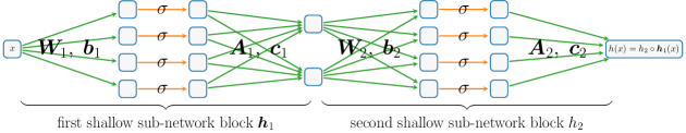
(a) MMNN of size $(4,2,2)$, i.e., width $4$, rank 2, and depth $2$.

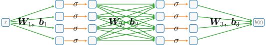
(b) FCNN of size $(4,2,3)$, i.e., width $4$ and depth $2$.

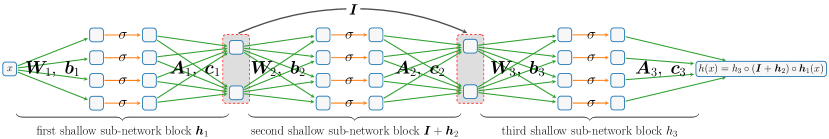
(c) ResMMNN of size $(4,2,3)$, i.e., width $4$, rank 2, and depth $3$.

Figure 1: Illustrations of $\sigma$-activated MMNN, FCNN, and ResMMNN.

2.3 Learning strategy of MMNNs

Our learning strategy is motivated by the following basic principle: a function can be decomposed in a multi-component and multi-layer structure each component of which can be approximated and trained effectively using a one-hidden-layer network, which is a linear combination of random basis functions (e.g., of the form $\sigma({\bm{W}}_{i}\cdot{\bm{x}}+{\bm{b}}_{i})$, see Section 3). Hence optimizing the linear combination weights of the random basis functions, i.e., ${\bm{A}}_{i},{\bm{c}}_{i}$ is both efficient and adequate. On the other hand, optimizing the weights (orientations of the basis functions) ${\bm{W}}_{i}$’s and biases ${\bm{b}}_{i}$’s to make the basis functions more adaptive to fine features of the target function, which would require capturing high-frequency information by a single layer network, leads to not only significantly more parameters to optimize but also difficulties in training as shown in [38]. Specifically, for each layer of MMNN, we fix the activation function parameters ($\bm{W}_{i}$’s and $\bm{b}_{i}$’s) as per PyTorch’s default setting during the training process. This entails initializing both weights and biases uniformly from the distribution $\mathcal{U}(-\sqrt{k},\sqrt{k})$, where $k=\frac{1}{\text{in\_features}}$. The whole training process optimizes all ${\bm{A}}_{i}$’s and ${\bm{c}}_{i}$’s simultaneously using Adam. Note that it is important to have a uniform sampling of orientations ${\bm{W}}_{i}$ and biases ${\bm{b}}_{i}$ for the random basis functions to be able to approximate an arbitrary smooth function well. Unless stated otherwise, parameter initialization adheres to the default settings provided by PyTorch in our experiments.

To demonstrate the advantages of our training approach (labeled S1), we conduct a comparison with the typical strategy in deep neural networks, denoted as Strategy S2, which uses the default PyTorch initialization and optimizes all parameters during training. In our tests, we select an oscillatory target function $f(x)=\cos(36\pi x^{2})-0.6\cos(12\pi x^{2})$ and use fairly compact networks. The tests are performed on a total of $1000$ uniform samples in $[-1,1]$ with a mini-batch size of $100$ and a learning rate for epoch-$k$ set at $0.001\times 0.9^{\lfloor k/400\rfloor}$ for $k=1,2,\mathinner{\mkern-0.1mu\cdotp\mkern-0.3mu\cdotp\mkern-0.3mu\cdotp\mkern-0.1mu},20000$, where $\lfloor\cdot\rfloor$ denotes the floor operation. The Adam optimizer [14] is applied throughout the training process.

Table 1: Comparison of test errors averaged over the last 100 epochs.

network	(width, rank, depth)	#parameters (trained / all)	test error (MSE)	test error (MAX)	training time
MMNN1 (S1)	(400, 20, 6)	40501 / 83301	$2.01\times 10^{-5}$	$4.36\times 10^{-2}$	23.9s / 1000 epochs
MMNN1 (S2)	(400, 20, 6)	83301 / 83301	$4.26\times 10^{-5}$	$4.71\times 10^{-2}$	30.2s / 1000 epochs
MMNN2 (S1)	(590, 28, 6)	83331 / 170061	$1.39\times 10^{-5}$	$2.80\times 10^{-2}$	25.2s / 1000 epochs

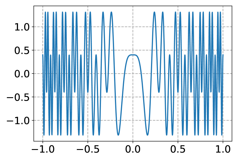
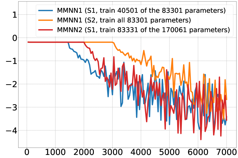
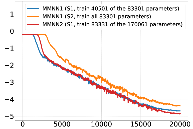
Figure 2: Left: target function $f(x)=\cos(36\pi x^{2})-0.6\cos(12\pi x^{2})$. Middle: logarithm of test errors vs. epoch. Right: logarithm of “test-error-aver” vs. epoch, where “test-error-aver” for epoch $k$ is calculated by averaging the errors in epochs $\max\{1,k-100\}$ to $\min\{k+100,\#\text{epochs}\}$.

As illustrated in Table 1 and Figure 2, our learning strategy S$1$ is significantly more effective than strategy S$2$ with comparable accuracy. There are two main advantages of S1. First, S1 requires training only about half the number of parameters compared to S2, which results in time savings. Second, S1 converges more quickly and performs significantly better when the training is not sufficient. We would like to note that in certain specific cases, S2 may outperform S1, particularly when the network size is relatively small and S2 is well-trained. This is expected since S$2$ trains all parameters, whereas S$1$ only trains a subset. Based on our experience, S1 is more effective in practice, particularly for sufficiently large networks. Alternatively, one might consider a hybrid learning strategy.

2.4 MMNNs versus FCNNs

Previously in Section 1, we discussed the theoretical differences between MMNNs and FCNNs. Now, let’s explore and compare their numerical performance. To ensure a fair comparison, we will use networks with a similar number of parameters, ensuring that all networks have sufficient parameters to learn the target function effectively. Typically, when training an FCNN, all parameters are optimized. For a thorough comparison, we will employ two learning strategies for MMNNs as detailed in Section 2.3: S1 and S2. S1 involves training approximately half the number of parameters of the MMNN, while S2 involves training all parameters.

We choose a 1D function $f_{1}(x)=\cos(20\pi|x|^{1.4})+0.5\cos(12\pi|x|^{1.6})$ and a 2D function

$$f_{2}(x_{1},x_{2})=\sum_{i=1}^{2}\sum_{j=1}^{2}a_{ij}\sin(sb_{i}x_{i}+sc_{ij}x_{i}x_{j})\cos(sb_{j}x_{j}+sd_{ij}x_{i}^{2}),$$

where $s=2$ and

$$(a_{i,j})=\begin{bmatrix}0.3&0.2\\ 0.2&0.3\end{bmatrix},\qquad(b_{i})=\begin{bmatrix}2\pi\\ 4\pi\end{bmatrix},\qquad(c_{i,j})=\begin{bmatrix}2\pi&4\pi\\ 8\pi&4\pi\end{bmatrix},\quad\textnormal{and}\quad(d_{i,j})=\begin{bmatrix}4\pi&6\pi\\ 8\pi&6\pi\end{bmatrix}.$$

Refer to Figures 4 and 4 for illustrations of $f_{1}$ and $f_{2}$, respectively.

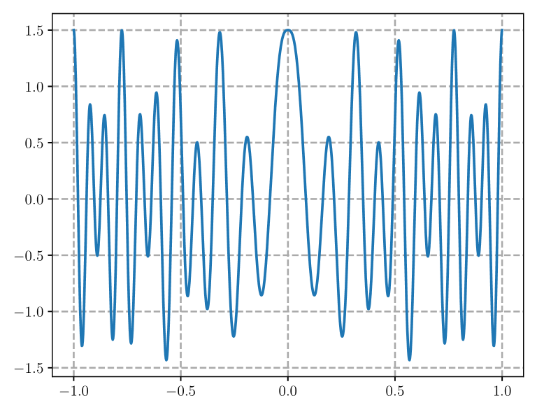
Figure 3: $f_{1}$.

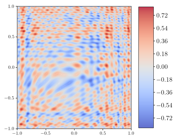
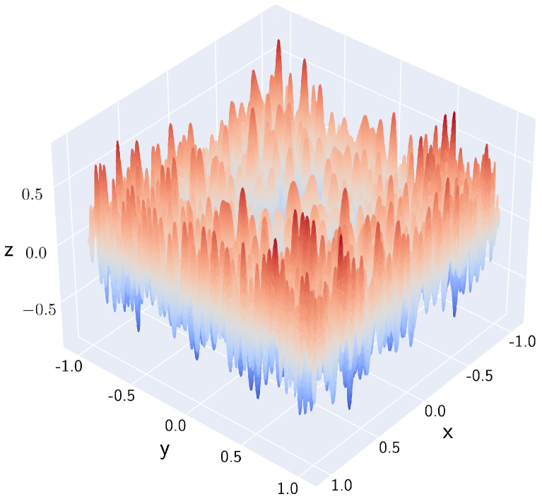
Figure 4: $f_{2}$.

We select large network sizes (see Table 2) to ensure that all networks possess sufficient parameters to learn the target functions. For training the 1D function, we sample a total of 1000 data points on a uniform grid within $[-1,1]$, using a mini-batch size of 100 and a learning rate of $0.001\times 0.9^{\lfloor k/400\rfloor}$ for epochs $k=1,2,\mathinner{\mkern-0.1mu\cdotp\mkern-0.3mu\cdotp\mkern-0.3mu\cdotp\mkern-0.1mu},20000$. For training the 2D function, we sample a total of $600^{2}$ data points on a uniform grid within $[-1,1]^{2}$, using a mini-batch size of 1000 and a learning rate of $0.001\times 0.9^{\lfloor k/16\rfloor}$ for epochs $k=1,2,\mathinner{\mkern-0.1mu\cdotp\mkern-0.3mu\cdotp\mkern-0.3mu\cdotp\mkern-0.1mu},800$.

Table 2: Comparison of test errors averaged over the last 100 epochs.

target function	network	(width, rank, depth)	#parameters (trained / all)	test error (MSE)	test error (MAX)	training time
$f_{1}$	MMNN1 (S1)	(388, 18, 6)	35399 / 73035	$2.49\times 10^{-6}$	$9.93\times 10^{-3}$	23.3s / 1000 epochs
$f_{1}$	FCNN1-1	(83, –, 6)	35110 / 35110	$2.43\times 10^{-4}$	$1.87\times 10^{-1}$	19.5s / 1000 epochs
$f_{1}$	MMNN1 (S2)	(388, 18, 6)	73035 / 73035	$2.05\times 10^{-6}$	$1.88\times 10^{-2}$	27.4s / 1000 epochs
$f_{1}$	FCNN1-2	(120, –, 6)	72961 / 72961	$1.73\times 10^{-4}$	$1.14\times 10^{-1}$	22.3s / 1000 epochs
$f_{2}$	MMNN2 (S1)	(789, 36, 12)	313630 / 637120	$4.61\times 10^{-6}$	$1.55\times 10^{-2}$	30.3s / 10 epochs
$f_{2}$	FCNN2-1	(168, –, 12)	312985 / 312985	$2.42\times 10^{-4}$	$2.75\times 10^{-1}$	26.7s / 10 epochs
$f_{2}$	MMNN2 (S2)	(789, 36, 12)	637120 / 637120	$6.17\times 10^{-6}$	$6.05\times 10^{-2}$	35.8s / 10 epochs
$f_{2}$	FCNN2-2	(240, –, 12)	637201 / 637201	$3.28\times 10^{-5}$	$1.39\times 10^{-1}$	29.3s / 10 epochs

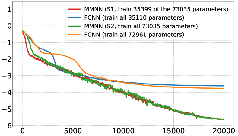
(a) $f_{1}$.

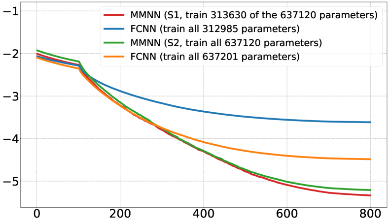
(b) $f_{2}$.

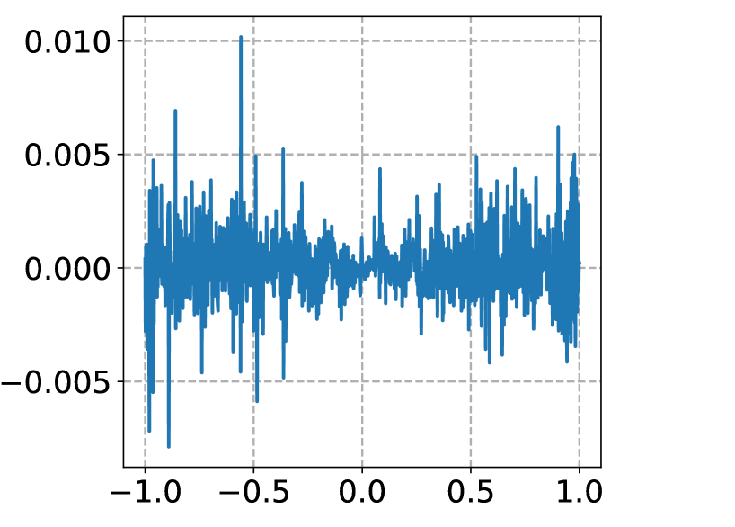
(c) MMNN1 (S1).

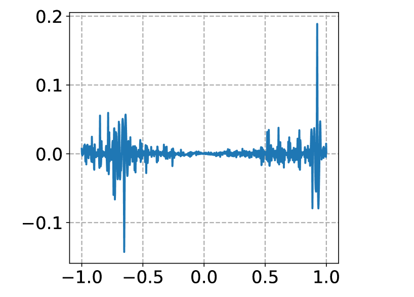
(d) FCNN1-1.

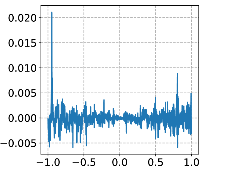
(e) MMNN1 (S2).

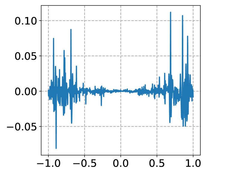
(f) FCNN1-2.

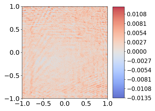
(g) MMNN2 (S1).

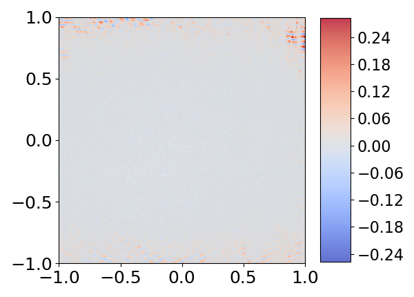
(h) FCNN2-1.

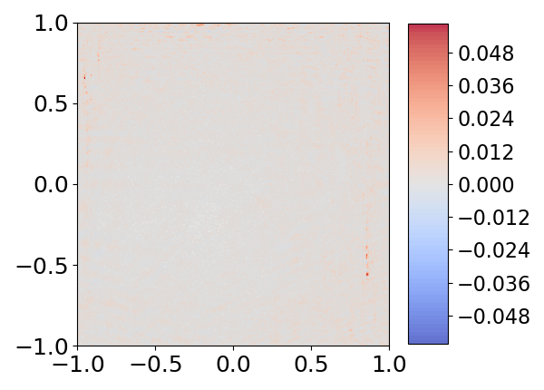
(i) MMNN2 (S2).

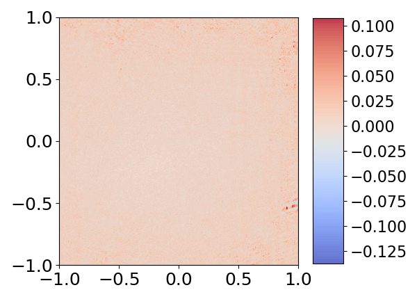
(j) FCNN2-2.

Figure 5: First row: logarithm of “test-error-aver” vs. epoch, where “test-error-aver” for epoch $k$ is calculated by averaging the errors in epochs $\max\{1,k-100\}$ to $\min\{k+100,\#\text{epochs}\}$. Second row: differences between learned networks and $f_{1}$. Second row: differences between learned networks and $f_{2}$.

As illustrated in Table 2 and Figure 5, MMNNs outperform FCNNs when both have the same depth and a comparable number of parameters, particularly for relatively oscillatory target functions. Moreover, as indicated in Table 2, the training time for MMNN (S1) is similar to that of FCNN, while MMNN (S2) takes a bit more time. We remark that the primary advantage of MMNNs lies in capturing high-frequency components. As we can see from Figure 5, the differences between network approximations and the corresponding target functions show that FCNNs approximate high-frequency parts of the target functions poorly. In contrast, the approximation errors for MMNNs, especially with the S1 learning strategy, are more evenly distributed across the entire domain, indicating their effectiveness in capturing high-frequency components. The Adam optimizer [14] is applied throughout the training process.

3 Multi-component and multi-layer decomposition

Although a one-hidden-layer neural network is a low-pass filter that can not represent and learn high-frequency features effectively [38], we use mathematical construction to show that MMNNs, which are composed of one-hidden-layer neural networks, can overcome this difficulty by decomposition of the complexity through components and/or depth. We emphasize that the decomposition is highly non-unique. Our construction is “man-made” which can be different from the one by computer through an optimization (learning) process. Our discussion begins with one-dimensional construction in Section 3.1 and later extends to higher dimensions in Section 3.2.

3.1 One dimensional construction

We begin with a two-component decomposition in 1D as both an illustration and an example in Section 3.1.1. Later in Section 3.1.2, we introduce the general multi-component decomposition. Finally in Section 3.1.3, we use concrete examples for demonstration.

3.1.1 Two-component decomposition

We show a simple “divide and conquer” strategy for a target function (example) $f(x)=\cos(2n\pi x)$, a high frequency Fourier mode when $n$ is large. Define

$${\bm{f}}_{1}:[-1,1]\mapsto[-1,1]^{2},\qquad{\bm{f}}_{1}=\begin{bmatrix}f_{1,1}\\ f_{1,2}\end{bmatrix},$$

$$f_{1,1}(x)={\mathtt{ReLU}}(2x)-1=\begin{cases}-1&\textnormal{for}\ x\in[-1,0),\\ 2x-1&\textnormal{for}\ x\in[0,1],\end{cases}$$

$$f_{1,2}(x)=-{\mathtt{ReLU}}(-2x)+1=\begin{cases}2x+1&\textnormal{for}\ x\in[-1,0),\\ 1&\textnormal{for}\ x\in[0,1],\end{cases}$$

and

$$f_{2}:(u,v)\in[-1,1]^{2}\mapsto\cos\big{(}n\pi(u+1)\big{)}+\cos\big{(}n\pi(v-1)\big{)}\in{\mathbb{R}}.$$

Then for any $x\in[-1,1]$ we have

$$\begin{split}f(x)&=\cos\Big{(}n\pi\cdot{\mathtt{ReLU}}(2x)\Big{)}+\cos\Big{(}-n\pi\cdot{\mathtt{ReLU}}(-2x)\Big{)}\\ &=\cos\Big{(}n\pi\big{(}f_{1,1}(x)+1\big{)}\Big{)}+\cos\Big{(}n\pi\big{(}f_{1,2}(x)-1\big{)}\Big{)}=f_{2}\circ{\bm{f}}_{1}(x)\end{split}$$

Through this decomposition and piecewise linear transformation, which can be approximated easily by a single layer of $\mathtt{ReLU}$ network, one only needs to approximate a function that is smoother than the original $f$: $\bm{f}_{1}$ is simplified, while $f_{2}$ is reduced to half of the frequency of the original target function $f$.

We observe that this decomposition approach is universally applicable for any function $f:[-1,1]\mapsto\mathbb{R}$. Specifically, the decomposition is defined as

$${\bm{f}}_{1}:[-1,1]\mapsto[-1,1]^{2},\qquad{\bm{f}}_{1}=\begin{bmatrix}f_{1,1}\\ f_{1,2}\end{bmatrix},$$

where the component functions $f_{1,1}$ and $f_{1,2}$ are defined by

$$f_{1,1}(x)={\mathtt{ReLU}}(2x)-1=\begin{cases}-1&\textnormal{for}\ x\in[-1,0),\\ 2x-1&\textnormal{for}\ x\in[0,1],\end{cases}$$

and

$$f_{1,2}(x)=-{\mathtt{ReLU}}(-2x)+1=\begin{cases}2x+1&\textnormal{for}\ x\in[-1,0),\\ 1&\textnormal{for}\ x\in[0,1].\end{cases}$$

Moreover,

$$f_{2}:(u,v)\in[-1,1]^{2}\mapsto f\big{(}\tfrac{u+1}{2}\big{)}+f\big{(}\tfrac{v-1}{2}\big{)}-f(0)\in{\mathbb{R}}.$$

Hence, for any $x\in[-1,1]$, we achieve the following reconstruction of $f(x)$:

$$\begin{split}f(x)&=f\Big{(}\tfrac{{\mathtt{ReLU}}(2x)}{2}\Big{)}+f\Big{(}\tfrac{-{\mathtt{ReLU}}(-2x)}{2}\Big{)}-f(0)\\ &=f\Big{(}\tfrac{f_{1,1}(x)+1}{2}\Big{)}+f\Big{(}\tfrac{f_{1,2}(x)-1}{2}\Big{)}-f(0)=f_{2}\circ{\bm{f}}_{1}(x)\end{split}$$

demonstrating a structured decomposition that allows the function to be expressed through the composition of a smoother function with a piecewise (component-wise) transformation and rescaling.

3.1.2 General multi-component decomposition

Now we propose a general multi-component adaptive decomposition, a “divide and conquer” strategy, that can distribute the complexity of a target function evenly to multiple components.

Given a sequence $x_{0}<x_{1}<\mathinner{\mkern-0.1mu\cdotp\mkern-0.3mu\cdotp\mkern-0.3mu\cdotp\mkern-0.1mu}<x_{n}$ where the target function is defined on the interval $[x_{0},x_{n}]$, we will demonstrate how our new architecture allows us to partition the complexities of the function $f$ into smaller intervals $[x_{i-1},x_{i}]$. By rescaling each subinterval, one only needs to deal with a much smoother function in each interval. This approach enables us to effectively approximate the target function over the entire interval $[x_{0},x_{n}]$.

Let ${\mathcal{L}}_{i}:[a_{i},b_{i}]\to[x_{i-1},x_{i}]$ be the linear map with

$${\mathcal{L}}_{i}(a_{i})=x_{i-1}\quad\textnormal{and}\quad{\mathcal{L}}_{i}(b_{i})=x_{i}.$$ (2)

Define

$$f_{i}=f\circ{\mathcal{L}}_{i}:[a_{i},b_{i}]\to{\mathbb{R}}.$$ (3)

To decompose the target function into smoother pieces, we define a piecewise linear transformation $\psi_{i}$ using a linear combination of two ReLU functions (or a simple single layer network),

$$\psi_{i}(x)=s_{i}\cdot{\mathtt{ReLU}}\left({x-x_{i-1}}\right)-s_{i}\cdot{\mathtt{ReLU}}\left({x-x_{i}}\right)+a_{i}.$$ (4)

Here $s_{i}=\frac{b_{i}-a_{i}}{x_{i}-x_{i-1}}$ is the “slope” of ${\mathcal{L}}_{i}^{-1}$, which is a local rescaling. For example, $f_{i}$ becomes a smoother function than $f$ after stretching $[x_{i-1},x_{i}]$ to a larger domain $[a_{i},b_{i}]$. See an illustration of $\psi_{i}(x)$ in Figure 6.

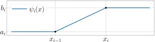
Figure 6: An illustration of $\psi_{i}(x)$.

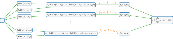
(a) Decompostion of target function $f=c+\sum_{i=1}^{n}f_{i}\circ\psi_{i}$: oscillatory $f$ to smooth $f_{i}$’s.

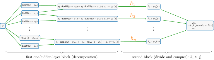
(b) Neural network architecture of $h=c+\sum_{i=1}^{n}h_{i}\circ\psi_{i}$ by using $h_{i}\approx f_{i}$.

Figure 7: Visual representations of the decompositions of $f$ and $h$ are provided with $c=\sum_{i=0}^{n-1}f(x_{i})$ being a constant and $s_{i}$ being the slope. Here, the function $f$ is dissected into several simpler functions, labeled as $f_{i}$. Each $f_{i}$ represents a simplified and more manageable segment of $f$, allowing for the straightforward application of subnetwork $h_{i}$ to closely approximate $f_{i}$, even with the use of shallow networks.

Theorem 3.1.

Given $x_{0}<x_{1}<\mathinner{\mkern-0.1mu\cdotp\mkern-0.3mu\cdotp\mkern-0.3mu\cdotp\mkern-0.1mu}<x_{n}$, suppose ${\mathcal{L}}_{i}$ and $\psi_{i}$ are given in Equations (2) and (4), respectively. Then the target function $f:[x_{0},x_{n}]\to{\mathbb{R}}$ has the following (smoother) decomposition ($f_{i}$) with a piecewise linear transformation ($\psi_{i}$),

$$\begin{split}f(x)=\sum_{i=1}^{n}f_{i}\circ\psi_{i}(x)-\underbrace{\sum_{i=1}^{n-1}f(x_{i})}_{\textnormal{constant}}\quad\textnormal{for any $x\in[x_{0},x_{n}]$,}\end{split}$$

where $f_{i}$ is given in Equation (3).

Proof of Theorem 3.1.

By definition of $\psi_{i}$ in Equation (4), it is easy to check

$$\psi_{i}(x)=\begin{cases}b_{i}&\textnormal{if }x>x_{i},\\ {\mathcal{L}}_{i}^{-1}(x)&\textnormal{if }x\in[x_{i-1},x_{i}],\\ a_{i}&\textnormal{if }x<x_{i-1},\end{cases}\quad\Longrightarrow\quad\psi_{i}(x)=\begin{cases}b_{i}&\textnormal{if }i\leq j-1,\\ {\mathcal{L}}_{j}^{-1}(x)&\textnormal{if }i=j,\\ a_{i}&\textnormal{if }i\geq j+1,\end{cases}$$

for a fixed $j\in\{1,2,\mathinner{\mkern-0.1mu\cdotp\mkern-0.3mu\cdotp\mkern-0.3mu\cdotp\mkern-0.1mu},n\}$ and any $x\in[x_{j-1},x_{j}]$. It follows that

$$\begin{split}\sum_{i=1}^{n}f_{i}\circ\psi_{i}(x)&=\sum_{i=1}^{n}f\circ{\mathcal{L}}_{i}\circ\psi_{i}(x)=\sum_{i=1}^{j-1}f\circ{\mathcal{L}}_{i}\circ\psi_{i}(x)+f\circ{\mathcal{L}}_{j}\circ\psi_{j}(x)+\sum_{i=j+1}^{n}f\circ{\mathcal{L}}_{i}\circ\psi_{i}(x)\\ &=\sum_{i=1}^{j-1}f\circ{\mathcal{L}}_{i}(b_{i})+f\circ{\mathcal{L}}_{j}\circ{\mathcal{L}}_{j}^{-1}(x)+\sum_{i=j+1}^{n}f\circ{\mathcal{L}}_{i}(a_{i})\\ &=\sum_{i=1}^{j-1}f(x_{i})+f(x)+\sum_{i=j+1}^{n}f(x_{i-1})=f(x)+\underbrace{\sum_{i=1}^{n-1}f(x_{i})}_{\textnormal{constant}}.\end{split}$$

It follows that

$$\begin{split}f(x)=\sum_{i=1}^{n}f_{i}\circ\psi_{i}(x)-\underbrace{\sum_{i=1}^{n-1}f(x_{i})}_{\textnormal{constant}}\quad\textnormal{for any $x\in[x_{j-1},x_{j}]$.}\end{split}$$

Since $j$ is arbitrary, the above equation holds for all $x=\cup_{j=1}^{n}[x_{j-1},x_{j}]=[x_{0},x_{n}]$. ∎

For each smoother $f_{i}$, one can use a shallow network component $\phi_{i}$- a linear combination of random basis functions to approximate $f_{i}$ well on $[a_{i},b_{i}]$. Then

$$f(x)=\sum_{i=1}^{n}f_{i}\circ\psi_{i}(x)-\underbrace{\sum_{i=1}^{n-1}f(x_{i})}_{\textnormal{constant}}\approx\sum_{i=1}^{n}\phi_{i}\circ\psi_{i}(x)-\underbrace{\sum_{i=1}^{n-1}f(x_{i})}_{\textnormal{constant}}\eqqcolon h(x),$$

$h(x)$ is a one-hidden-layer neural network approximation of the target function $f(x)$ that can approximate a complex function better than a single layer. See Figure 7 for an illustration. In practice, one can choose repeated decomposition using a multi-component and multi-layer network structure which is the motivation for MMNN. It is well-known that neural networks can approximate smooth functions well. For localized rapid change/oscillation, our construction shows that a small network in terms of the width as well as the number of components and layers can achieve adaptive decomposition and deal with it rather easily. Hence MMNN is effective in approximating a function with localized fine features. This is an important advantage in dealing with low-dimensional structures embedded in high dimensions. The most difficult situation is approximating global highly oscillatory functions, especially with diverse frequency modes, for which wider networks with more components and layers are needed to deal with both the complexity and curse of dimensions.

3.1.3 Examples

Here we use two examples to demonstrate the complexity decomposition strategy presented in the previous section. We start with the Runge function $f(x)=\frac{1}{25x^{2}+1}$ and modify it to $f(x)=\frac{1}{1000x^{2}+1}$, which has a localized rapid change near $0$. As an example, we use four components $n=4$, choose points $x_{0},x_{1},x_{2},x_{3},x_{4}$ at $-1,-0.2,0,0.2,1$, and let $a_{i}=-1$ and $b_{i}=1$ for all $i$. In practice, each component is approximated by a single-layer network - a linear combination of basis functions, and trained by an optimization method, e.g., Adam. Our examples here are just a proof of concept for the decomposition of a target function into smoother components using MMNN structure in the form

$$f(x)=\sum_{i=1}^{4}f_{i}\circ\psi_{i}(x)-\underbrace{\sum_{i=1}^{3}f(x_{i})}_{\text{constant}},$$

where $f_{i}$ and $\psi_{i}$ (piecewise tranformation/rescaling) are defined as in (3) and (4), respectively. These components are illustrated in Figure 8. Each component is relatively smooth, making it easier for approximation and learning through shallow networks. This approach essentially utilizes a divide-and-conquer principle.

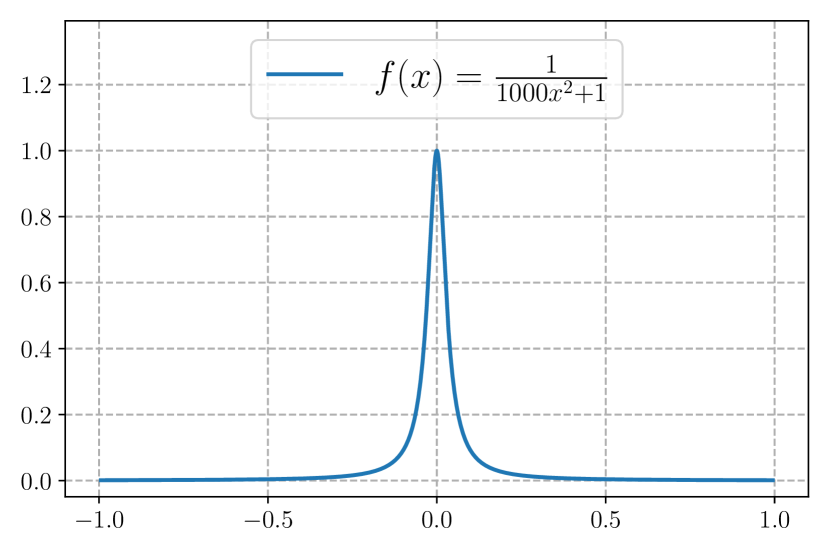
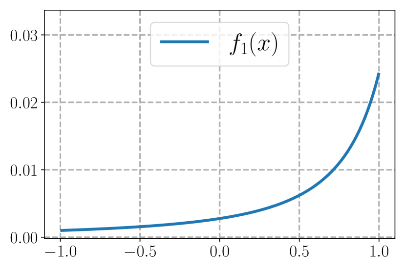
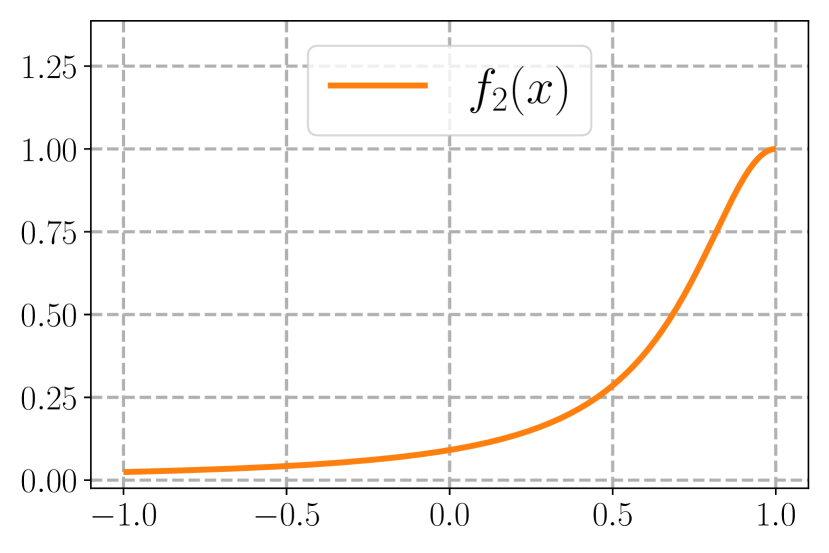
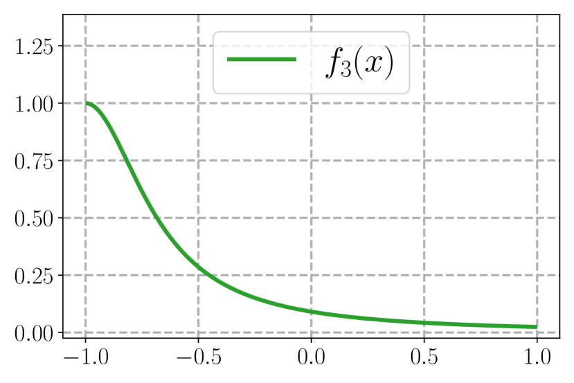
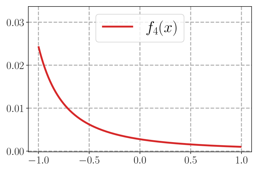
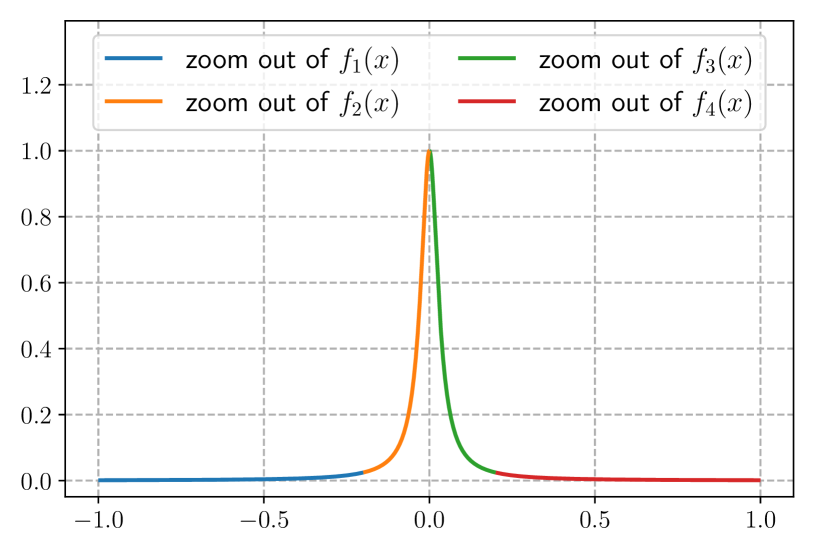
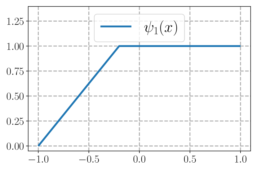
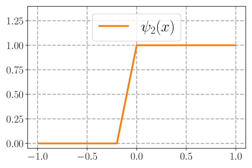
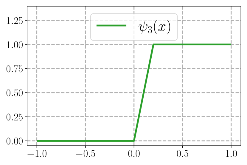
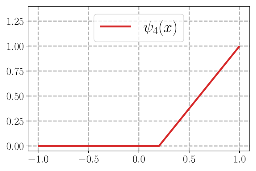
Figure 8: Illustrations of $f(x)=\frac{1}{1000x^{2}+1}$ and its multi-component decomposition through $f_{i}$ and $\psi_{i}$ $i=1,2,3,4$, where $f(x)=\sum_{i=1}^{4}f_{i}\circ\psi_{i}(x)-{\sum_{i=1}^{3}f(x_{i})}$.

The second example is a globally oscillatory function of the form

$$f(x)=\cos^{2}(6\pi x)+\sin(10\pi x^{2}).$$

Again we illustrate using four components $n=4$, selecting points $x_{0},x_{1},x_{2},x_{3},x_{4}$ at $-1,-0.7,0,0.7,1$, and setting $a_{i}=-1$ and $b_{i}=1$ for all $i$. As shown in Figure 9, the target function $f(x)$ is decomposed into components that are less oscillatory again facilitating their approximation and learning through shallow networks.

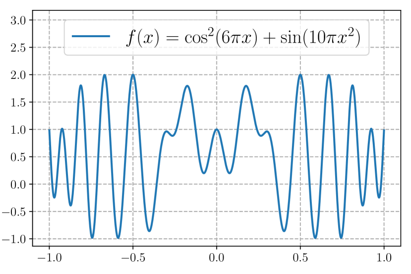
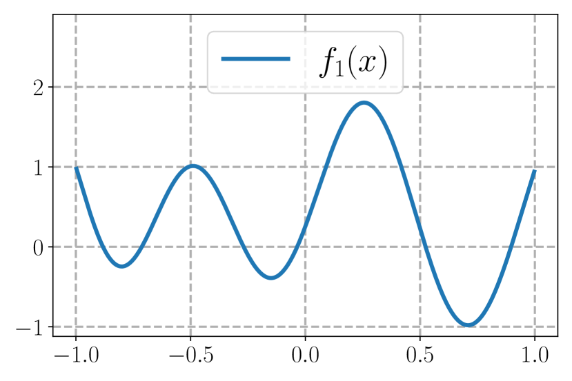
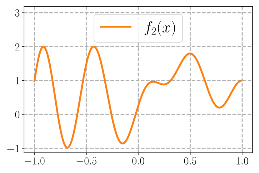
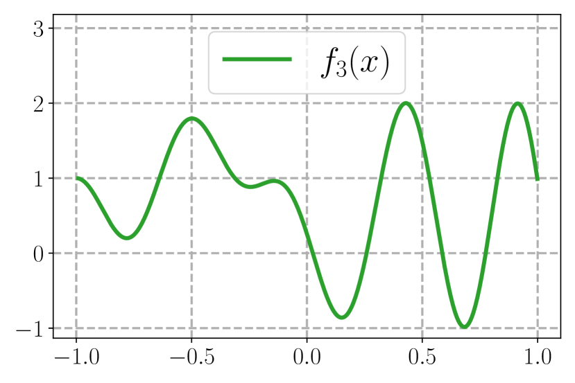
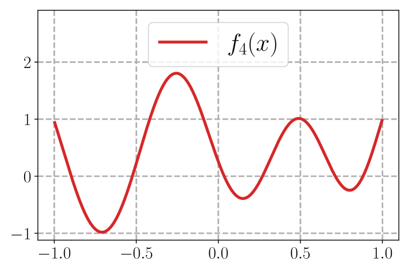
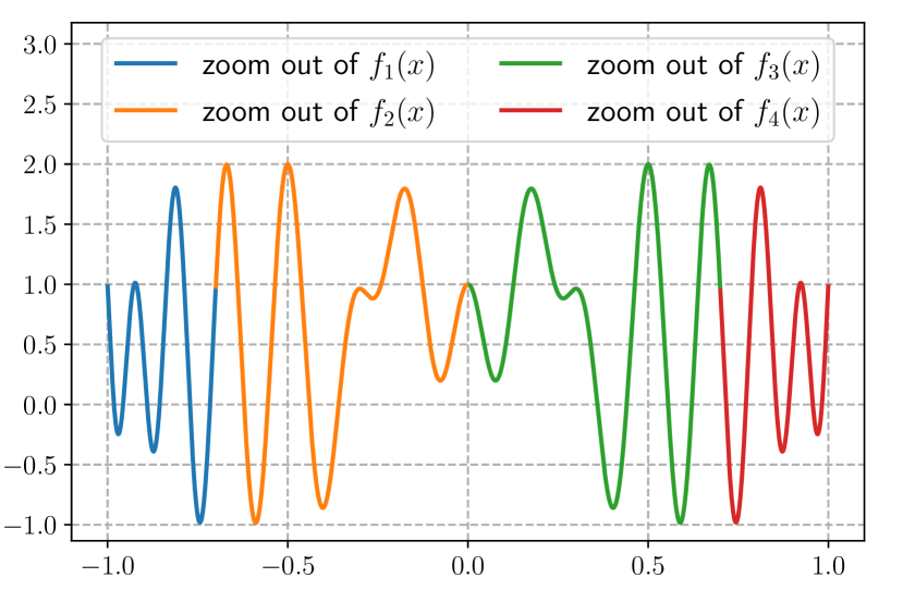
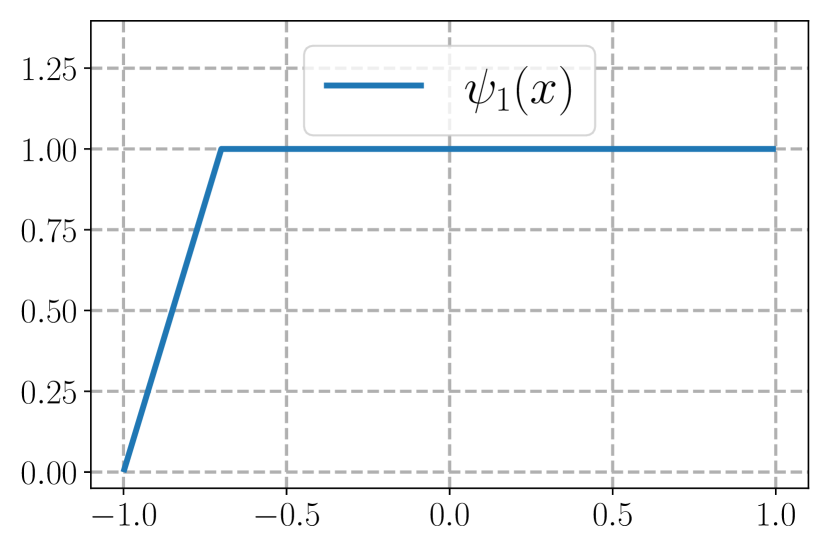
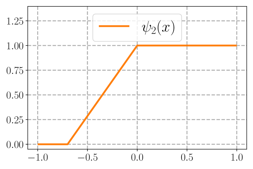
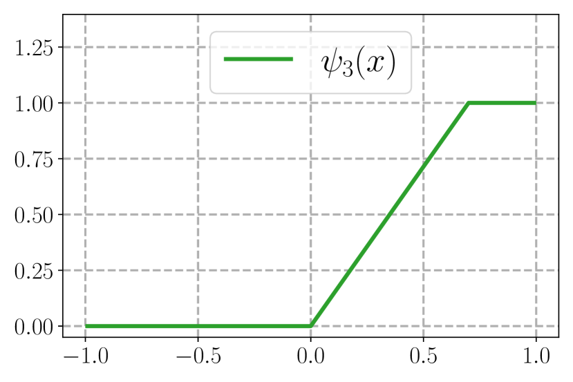
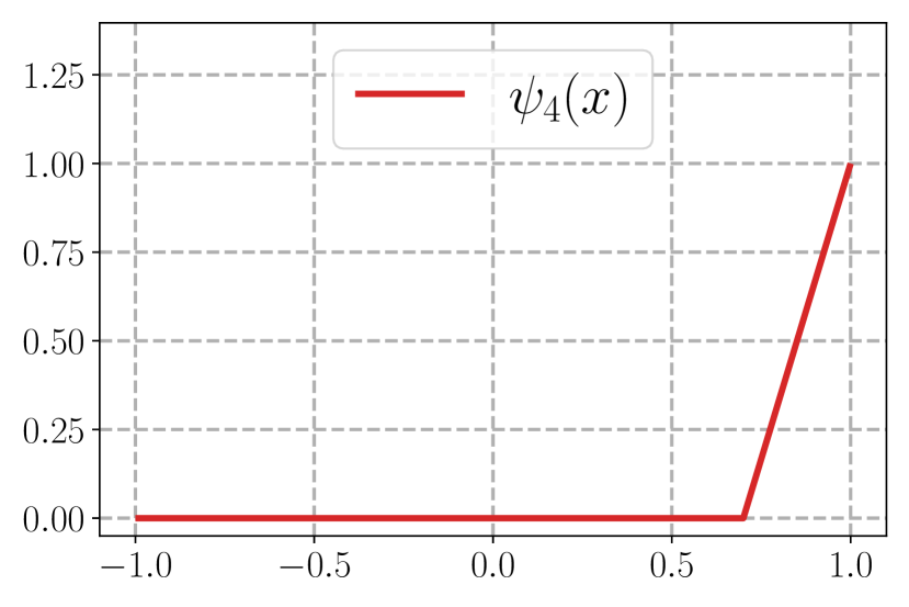
Figure 9: Illustrations of $f(x)=\cos^{2}(6\pi x)+\sin(10\pi x^{2})$ and its decomposition components $f_{i}$ and $\psi_{i}$ such that $f(x)=\sum_{i=1}^{4}f_{i}\circ\psi_{i}(x)-{\sum_{i=1}^{3}f(x_{i})}$.

3.2 High dimensional cases

Let us now consider the extension to multi-dimension using two dimensions as an example since the simple dimension-by-dimension strategy applies to any dimension.

Given $x_{0}<x_{1}<\mathinner{\mkern-0.1mu\cdotp\mkern-0.3mu\cdotp\mkern-0.3mu\cdotp\mkern-0.1mu}<x_{n}$ and $y_{0}<y_{1}<\mathinner{\mkern-0.1mu\cdotp\mkern-0.3mu\cdotp\mkern-0.3mu\cdotp\mkern-0.1mu}<y_{m}$, dividing the domain of the function $f(x,y)$ into small Cartesian rectangles $[x_{i-1},x_{i}]\times[y_{j-1},y_{j}]$. Let ${\mathcal{L}}_{1,i}:[a_{i},b_{i}]\to[x_{i-1},x_{i}]$ and ${\mathcal{L}}_{2,j}:[c_{i},d_{i}]\to[y_{j-1},y_{j}]$ be the linear maps with

$$\begin{cases}{\mathcal{L}}_{1,i}(a_{i})=x_{i-1},\\ {\mathcal{L}}_{1,i}(b_{i})=x_{i}\end{cases}\quad\textnormal{and}\quad\,\ \begin{cases}{\mathcal{L}}_{2,j}(c_{i})=y_{j-1},\\ {\mathcal{L}}_{2,j}(d_{i})=y_{j}.\end{cases}$$ (5)

For $i=1,2,\mathinner{\mkern-0.1mu\cdotp\mkern-0.3mu\cdotp\mkern-0.3mu\cdotp\mkern-0.1mu},n$ and $j=1,2,\mathinner{\mkern-0.1mu\cdotp\mkern-0.3mu\cdotp\mkern-0.3mu\cdotp\mkern-0.1mu},m$, we define

$$\left\{\begin{array}[]{l}f_{i,0}(x,y)\coloneqq f\Big{(}{\mathcal{L}}_{1,i}(x),\,y\Big{)},\\ f_{0,j}(x,y)\coloneqq f\Big{(}x,\,{\mathcal{L}}_{2,j}(y)\Big{)},\\ f_{i,j}(x,y)\coloneqq f\Big{(}{\mathcal{L}}_{1,i}(x),\,{\mathcal{L}}_{2,j}(y)\Big{)}=f_{0,j}\Big{(}{\mathcal{L}}_{1,i}(x),\,y\Big{)}=f_{i,0}\Big{(}x,\,{\mathcal{L}}_{2,j}(y)\Big{)}.\end{array}\right.$$ (6)

It is evident that with appropriate transformation and rescaling, $f_{i,0}(x,y)$ is smooth in $x$ when $y$ is held constant, $f_{0,j}(x,y)$ is smooth in $y$ when $x$ is fixed, and $f_{i,j}(x,y)$ is smooth in both $x$ and $y$. Define

$$\psi_{i}(x)=\begin{cases}b_{i}&\textnormal{if }x>x_{i},\\ {\mathcal{L}}_{1,i}^{-1}(x)&\textnormal{if }x\in[x_{i-1},x_{i}],\\ a_{i}&\textnormal{if }x<x_{i-1}\end{cases}\quad\textnormal{and}\quad\phi_{j}(y)=\begin{cases}d_{j}&\textnormal{if }y>y_{j},\\ {\mathcal{L}}_{2,j}^{-1}(y)&\textnormal{if }y\in[y_{j-1},y_{j}],\\ c_{j}&\textnormal{if }y<y_{j-1}.\end{cases}$$ (7)

The following result provides a decomposition of $f$ that fits into the structure of MMNN.

Theorem 3.2.

Given $x_{0}<x_{1}<\mathinner{\mkern-0.1mu\cdotp\mkern-0.3mu\cdotp\mkern-0.3mu\cdotp\mkern-0.1mu}<x_{n}$ and $y_{0}<y_{1}<\mathinner{\mkern-0.1mu\cdotp\mkern-0.3mu\cdotp\mkern-0.3mu\cdotp\mkern-0.1mu}<y_{m}$, suppose ${\mathcal{L}}_{1,i},{\mathcal{L}}_{2,j}$ and $\psi_{i},\phi_{j}$ are given in Equations (5) and (7), respectively. Then the function $f:[x_{0},x_{n}]\times[y_{0},y_{m}]\to{\mathbb{R}}$ can be expressed as

$$\begin{split}f(x,\,y)&=\sum_{i=1}^{n}\sum_{j=1}^{m}f_{i,j}\Big{(}\psi_{i}(x),\,\phi_{j}(y)\Big{)}-\sum_{i=1}^{n}\sum_{j=1}^{m-1}f_{i,0}\Big{(}\psi_{i}(x),\,y_{j}\Big{)}\\ &\quad\ -\sum_{i=1}^{n-1}\sum_{j=1}^{m}f_{0,j}\Big{(}x_{i},\,\phi_{j}(y)\Big{)}+\sum_{i=1}^{n-1}\sum_{j=1}^{m-1}f(x_{i},\,y_{j})\end{split}$$ (8)

for all $(x,y)\in[x_{0},x_{n}]\times[y_{0},y_{m}]$, where $f_{i,j}$ are given in Equation (6).

Proof of Theorem 3.2.

Fixing $(k,j)$, for any $(x,y)\in[x_{k-1},x_{k}]\times[y_{\ell-1},y_{\ell}]$, we have

$$\psi_{i}(x)=\begin{cases}b_{i}&\textnormal{if }i\leq k-1,\\ {\mathcal{L}}_{1,k}^{-1}(x)&\textnormal{if }i=k,\\ a_{i}&\textnormal{if }i\geq k+1\end{cases}\quad\textnormal{and}\quad\phi_{j}(y)=\begin{cases}d_{j}&\textnormal{if }j\leq\ell-1,\\ {\mathcal{L}}_{2,\ell}^{-1}(y)&\textnormal{if }j=\ell,\\ c_{j}&\textnormal{if }j\geq\ell+1.\end{cases}$$

It follows that

$$\begin{split}&\phantom{=\;}\sum_{i=1}^{n}f_{i,0}\Big{(}\psi_{i}(x),\,y\Big{)}=\sum_{i=1}^{n}f\Big{(}{\mathcal{L}}_{1,i}\circ\psi_{i}(x),\,y\Big{)}\\ &=\sum_{i=1}^{k-1}f\Big{(}{\mathcal{L}}_{1,i}\circ\psi_{i}(x),\,y\Big{)}+f\Big{(}{\mathcal{L}}_{1,k}\circ\psi_{k}(x),\,y\Big{)}+\sum_{i=k+1}^{n}f\Big{(}{\mathcal{L}}_{1,i}\circ\psi_{i}(x),\,y\Big{)}\\ &=\sum_{i=1}^{k-1}f\Big{(}{\mathcal{L}}_{1,i}(b_{i}),\,y\Big{)}+f\Big{(}{\mathcal{L}}_{1,k}\circ{\mathcal{L}}_{1,k}^{-1}(x),\,y\Big{)}+\sum_{i=k+1}^{n}f\Big{(}{\mathcal{L}}_{1,i}(a_{i}),\,y\Big{)}\\ &=\sum_{i=1}^{k-1}f(x_{i},\,y)+f(x,\,y)+\sum_{i=k+1}^{n}f(x_{i-1},\,y)=f(x,\,y)+\sum_{i=1}^{n-1}f(x_{i},\,y),\end{split}$$

implying

$$\begin{split}f(x,\,y)=\sum_{i=1}^{n}f_{i,0}\Big{(}\psi_{i}(x),\,y\Big{)}-\sum_{i=1}^{n-1}f(x_{i},\,y).\end{split}$$

For each $i$, using the 1D decomposition technique described in Section 3.1, we find the decompositions for $f_{i,0}\big{(}\psi_{i}(x),\,y\big{)}$ and $f(x_{i},\,y)$. We have

$$\begin{split}&\phantom{=\;}\sum_{j=1}^{m}f_{i,j}\Big{(}\psi_{i}(x),\,\phi_{j}(y)\Big{)}=\sum_{j=1}^{m}f_{i,0}\Big{(}\psi_{i}(x),\,{\mathcal{L}}_{2,j}\circ\phi_{j}(y)\Big{)}\\ &=\sum_{j=1}^{\ell-1}f_{i,0}\Big{(}\psi_{i}(x),\,{\mathcal{L}}_{2,j}\circ\phi_{j}(y)\Big{)}+f_{i,0}\Big{(}\psi_{i}(x),\,{\mathcal{L}}_{2,\ell}\circ\phi_{\ell}(y)\Big{)}+\sum_{j=\ell+1}^{m}f_{i,0}\Big{(}\psi_{i}(x),\,{\mathcal{L}}_{2,j}(\circ\phi_{j}(y))\Big{)}\\ &=\sum_{j=1}^{\ell-1}f_{i,0}\Big{(}\psi_{i}(x),\,{\mathcal{L}}_{2,j}(d_{j})\Big{)}+f_{i,0}\Big{(}\psi_{i}(x),\,{\mathcal{L}}_{2,\ell}\circ{\mathcal{L}}_{2,\ell}^{-1}(y)\Big{)}+\sum_{j=\ell+1}^{m}f_{i,0}\Big{(}\psi_{i}(x),\,{\mathcal{L}}_{2,j}(c_{j})\Big{)}\\ &=\sum_{j=1}^{\ell-1}f_{i,0}\Big{(}\psi_{i}(x),\,y_{j}\Big{)}+f_{i,0}\Big{(}\psi_{i}(x),\,y\Big{)}+\sum_{j=\ell+1}^{m}f_{i,0}\Big{(}\psi_{i}(x),\,y_{j-1}\Big{)}\\ &=f_{i,0}\Big{(}\psi_{i}(x),\,y\Big{)}+\sum_{j=1}^{m-1}f_{i,0}\Big{(}\psi_{i}(x),\,y_{j-1}\Big{)},\end{split}$$

implying

$$\begin{split}f_{i,0}\Big{(}\psi_{i}(x),\,y\Big{)}=\sum_{j=1}^{m}f_{i,j}\Big{(}\psi_{i}(x),\,\phi_{j}(y)\Big{)}-\sum_{j=1}^{m-1}f_{i,0}\Big{(}\psi_{i}(x),\,y_{j}\Big{)}.\end{split}$$

Moreover,

$$\begin{split}&\phantom{=\;}\sum_{j=1}^{m}f_{0,j}\Big{(}x_{i},\,\phi_{j}(y)\Big{)}=\sum_{j=1}^{m}f\Big{(}x_{i},\,{\mathcal{L}}_{2,j}\circ\phi_{j}(y)\Big{)}\\ &=\sum_{j=1}^{\ell-1}f\Big{(}x_{i},\,{\mathcal{L}}_{2,j}\circ\phi_{j}(y)\Big{)}+f\Big{(}x_{i},\,{\mathcal{L}}_{2,\ell}\circ\phi_{\ell}(y)\Big{)}+\sum_{j=\ell+1}^{m}f\Big{(}x_{i},\,{\mathcal{L}}_{2,j}\circ\phi_{j}(y)\Big{)}\\ &=\sum_{j=1}^{\ell-1}f\Big{(}x_{i},\,{\mathcal{L}}_{2,j}(d_{j})\Big{)}+f\Big{(}x_{i},\,{\mathcal{L}}_{2,\ell}\circ{\mathcal{L}}_{2,\ell}^{-1}(y)\Big{)}+\sum_{j=\ell+1}^{m}f\Big{(}x_{i},\,{\mathcal{L}}_{2,j}(c_{j})\Big{)}\\ &=\sum_{j=1}^{\ell-1}f(x_{i},\,y_{j})+f(x_{i},\,y)+\sum_{j=\ell+1}^{m}f(x_{i},\,y_{j-1})=f(x_{i},\,y)+\sum_{j=1}^{m-1}f(x_{i},\,y_{j}),\end{split}$$

implying

$$\begin{split}f(x_{i},\,y)=\sum_{j=1}^{m}f_{0,j}\Big{(}x_{i},\,\phi_{j}(y)\Big{)}-\sum_{j=1}^{m-1}f(x_{i},\,y_{j}).\end{split}$$

Therefore, for any $(x,y)\in[x_{k-1},x_{k}]\times[y_{\ell-1},y_{\ell}]$,

$$\begin{split}&\phantom{=\;\;}f(x,\,y)=\sum_{i=1}^{n}f_{i,0}\Big{(}\psi_{i}(x),\,y\Big{)}-\sum_{i=1}^{n-1}f(x_{i},\,y)\\ &=\sum_{i=1}^{n}\Bigg{(}\sum_{j=1}^{m}f_{i,j}\Big{(}\psi_{i}(x),\,\phi_{j}(y)\Big{)}-\sum_{j=1}^{m-1}f_{i,0}\Big{(}\psi_{i}(x),\,y_{j}\Big{)}\Bigg{)}-\sum_{i=1}^{n-1}\Bigg{(}\sum_{j=1}^{m}f_{0,j}\Big{(}x_{i},\,\phi_{j}(y)\Big{)}-\sum_{j=1}^{m-1}f(x_{i},\,y_{j})\Bigg{)}\\ &=\sum_{i=1}^{n}\sum_{j=1}^{m}f_{i,j}\Big{(}\psi_{i}(x),\,\phi_{j}(y)\Big{)}-\sum_{i=1}^{n}\sum_{j=1}^{m-1}f_{i,0}\Big{(}\psi_{i}(x),\,y_{j}\Big{)}-\sum_{i=1}^{n-1}\sum_{j=1}^{m}f_{0,j}\Big{(}x_{i},\,\phi_{j}(y)\Big{)}+\sum_{i=1}^{n-1}\sum_{j=1}^{m-1}f(x_{i},\,y_{j}).\end{split}$$

Since $k$ and $\ell$ are arbitrary, the above equation holds for all $(x,y)=\cup_{k=1}^{n}\cup_{\ell=1}^{m}[x_{k-1},x_{k}]\times[y_{\ell-1},y_{\ell}]=[x_{0},x_{n}]\times[y_{0},y_{m}]$. ∎

3.3 Related work

Approximation

Extensive research has examined the approximation capabilities of neural networks, focusing on various architectures to approximate diverse target functions. Early studies concentrated on the universal approximation power of single-hidden-layer networks [3, 10, 11], which demonstrated that sufficiently large neural networks could approximate specific functions with arbitrary precision mathematically, without quantifying the error relative to network size. Subsequent research, such as [36, 35, 1, 39, 2, 6, 7, 21, 30, 31, 19, 32, 37, 33], analyzed the approximation error for different networks in terms of size characterized by width, depth, or the number of parameters. Those studies have primarily concentrated on the mathematical theory that supports the existence theory for such neural networks. However, there has been limited focus on determining the parameters within these networks computationally and the numerical errors, particularly those arising from finite precision in computer simulations. This gap motivated our current investigation, which considers practical training processes and numerical errors. Specifically, the balanced structure of MMNN, the choice of training parameters, and the associated learning strategy discussed here are intended to facilitate a smooth decomposition of the function, thereby promoting an efficient training process.

Low-rank methods

Low-rank structures in the weight matrix ${\bm{W}}$ of a fully connected neural network have been investigated by various groups. For example, the methods proposed in [26, 12, 28] focus on accelerating training and reducing memory requirements while maintaining final performance. The concept of low-rank structures is further extended to tensor train decomposition in [22]. The MMNN proposed here differs in two key aspects. First, each layer contains two matrices: ${\bm{A}}$ outside and ${\bm{W}}$ inside the activation functions. Each row of ${\bm{A}}$ represents the weights for a linear combination of a set of random basis functions, forming a component in each layer. The number of rows in ${\bm{A}}$, which equals the number of components, is selected based on the complexity of the function and is typically much smaller than the number of columns, corresponding to the number of basis functions. Each row of $({\bm{W}},{\bm{b}})$ represents a random parameterization of a basis function, with the number of rows in ${\bm{W}}$ corresponding to the number of basis functions, usually much larger than the number of columns in ${\bm{W}}$, which is the input dimension. Secondly, in our MMNN, only ${\bm{A}}$ is trained while ${\bm{W}}$ remains fixed with randomly initialized values. Theoretical studies and numerical experiments demonstrate that the architecture of MMNN, combined with the learning strategy, is effective in approximating complex functions.

Random features

Fixing $({\bm{W}},{\bm{b}})$ of each layer and use of random basis functions in the MMNNs is inspired by a previous approach known as random features [24, 34, 16, 27, 23]. In typical random feature methods, only the linear combination parameters at the output layer are trained which also leads to the issue of ill-conditioning of the representation. While in MMNNS matrix ${\bm{A}}$ and vector ${\bm{c}}$ of each layer are trained. Our MMNN employs a composition architecture and learning mechanism that enhances the approximation capabilities compared to random feature methods while achieving a more effective training process than a standard fully connected network of equivalent size. Extensive experiments demonstrate that our approach can strike a satisfactory balance between approximation accuracy and training cost.

Komogolrov-Arnold (KA) representation

The KA representation theorem [15] states that any multivariate continuous function on a hypercube can be expressed as a finite composition of continuous univariate functions and the binary operation of addition. However, this elegant mathematical representation may result in non-smooth or even fractal univariate functions in general due to this very specific form of representation, a computational challenge one has to address in practice. KA representation has been explored in several studies [17, 20, 32, 13]. A recently proposed network known as the KA network (KAN) utilizes spline functions to approximate the univariate functions in the KA representation. The proposed MMNN is motivated by a multi-component and multi-layer smooth decomposition, or a “divide and conquer” approach, employing distinct network architectures, activation functions, and training strategies.

4 Numerical experiments

In this section, we perform extensive experiments to validate our analysis and demonstrate the effectiveness of MMNNs through multi-component and multi-layer decomposition studied in Section 3. In particular, our tests show its ability in 1) adaptively capturing localized high-frequency features in Section 4.1, 2) approximating highly oscillatory functions in Section 4.2, and 3) extending to higher dimensions in Section 4.3 as well as some interesting learning dynamics in Section 4.4. All our experiments involve target functions that include high-frequency components in various ways and are difficult to handle by shallow networks (no matter how wide) as shown in our previous work [38]. Moreover, our experience on these tests shows that using a fully connected deep neural network would require many more parameters and is much harder (if possible) to train to get a comparable result. This is mainly due to a balanced and structured network design of MMNN in terms of 1) the network width $w$, which is the number of hidden neurons or random basis functions in each component, 2) the rank $r$, which is the number of components in each layer, and 3) the network depth $l$, which is the number of layers in the network. The use of a controllable number of collective components (through ${\bm{A}}$) in each layer instead of a large number of individual neurons and the use of fixed and randomly chosen weights $({\bm{W}},{\bm{b}})$ make the training process more effective.

In all tests, 1) data are sampled enough to resolve fine features in the target function, 2) the Adam optimizer is used in training, 3) mean squared error (MSE) is the loss function, 4) all parameters are initialized according to the PyTorch default initialization (see Section 2.3) unless otherwise specified, 5) ${\bm{W}}$’s and ${\bm{b}}$’s (the parameters inside the activation functions, see Section 2.2) are fixed and only ${\bm{A}}$’s and ${\bm{c}}$’s (the parameters outside the activation functions) are trained, 6) computations are conducted on an NVIDIA RTX 3500 Ada Generation Laptop GPU (power cap 130W), with most experiments concluding within a range from a few dozen to several thousand seconds. All our MMNN setups are specified by three parameters $(w,r,l)$ which depends on the function complexity. Another tuning parameter is the learning rate the choice of which is guided by the following criteria: 1) not too large initially due to stability, 2) a decreasing rate with iterations such that the learning rate becomes small near the equilibrium to achieve a good accuracy while not decreasing too fast (especially during a long training process for more difficult target functions) so that the training is stalled.

4.1 Localized rapid changes

We begin with two examples in 1D. The first is $f(x)=\arctan(100x+20)$, which is smooth but features a rapid transition at zero. While demonstrated in our previous work [38], a shallow network struggles to capture such a simple local fast transition which contains high-frequencies, we show that this function can be approximated easily by a composition of a smooth function on top of a (repeated) spatial decomposition and local rescaling using MMNN structure in Section 2.2. Our test indeed verifies that our new architecture can effectively capture a localized fast transition rather easily using a very small network of size $(16,4,3)$ as shown in Figure 11. For this test, a total of 1000 data points are uniformly sampled in the range $[-1,1]$, with a mini-batch size of 100, a learning rate of $10^{-3}$, and the number of epochs set to 2000. Figure 11 gives the error plot.

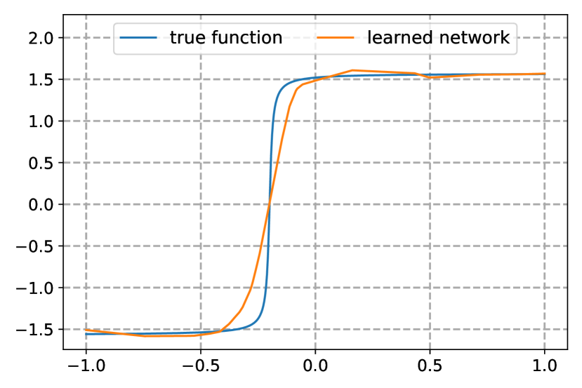
(a) Epoch 100.

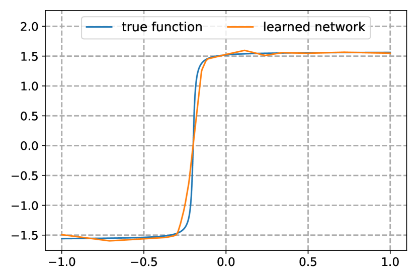
(b) Epoch 200.

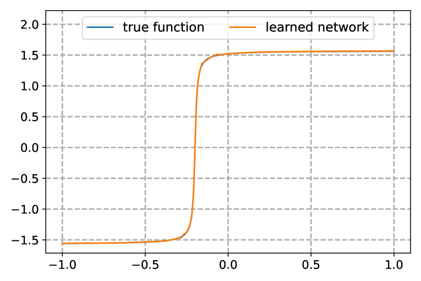
(c) Epoch 2000.

Figure 10: Illustrations of the training process.

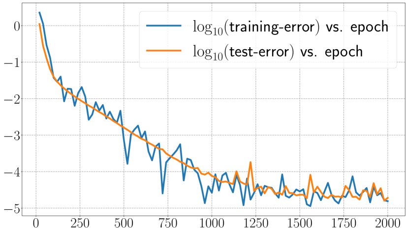
Figure 11: Training and test errors (MSE).

Next, we consider a more complicated target function, $f(x)={\mathds{1}}_{\{|x+0.2|<0.02\}}\cdot\sin(50\pi x)$, which represents a localized fast oscillation. For this example, we will conduct two tests. The first one is to show the flexibility of MMNN to automatically adapt to local features. The network has a small size as above $(16,4,3)$. Each layer has a network width of 16. In other words, each component is a linear combination of 16 ReLU functions which has no way to approximate such a target function well. However, with a multi-layer and multi-component decomposition with parameters appropriately trained by Adam, MMNN can adapt to the behavior of the target function as shown in Figure 12. Figure 14 gives the error plot. Also, the test shows that this example is more difficult to train. For this test, there are a total of 1000 uniformly sampled points in $[-1,1]$ with a mini-batch size of 100 and a learning rate of $0.002\times 0.95^{\lfloor k/1000\rfloor}$, where $\lfloor\cdot\rfloor$ denotes floor operation and $k=1,2,\mathinner{\mkern-0.1mu\cdotp\mkern-0.3mu\cdotp\mkern-0.3mu\cdotp\mkern-0.1mu},20000$ is the epoch number. It should be noted that in this test, we initialize the biases ${\bm{b}}$’s to $\bm{0}$ and use the PyTorch default initialization method for the weights ${\bm{W}}$. This approach, inspired by Xavier initialization, is chosen because the target function is locally oscillatory and the MMNN size is quite small, necessitating a setup adaptive to the target function to facilitate the training. For other experiments, both the biases and weights use the PyTorch default initialization. We then compare with least square approximation using uniform finite element method (FEM) basis with the same degrees of freedom. As shown in Figure 14, MMNN renders a better approximation due to automatic adaptation through the training process. We would like to remark that when training an extremely compact MMNN which does not have much flexibility and makes the training more subtle, the training hyperparameters, such as learning rate, min-batch size, and etc., need to be more carefully tuned. However, when there is some redundancy in MMNN, i.e., an MMNN with a slightly larger size, MMNN becomes more flexible and the training process becomes easier. On the other hand, when the network becomes too large, then training a large number of parameters and over-redundancy will lead to potential difficulties for optimization. This also shows that there is a trade-off between representation and optimization one needs to balance in practice.

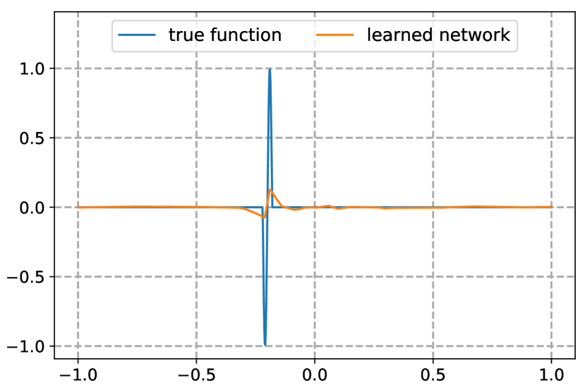
(a) Epoch 500.

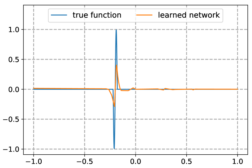
(b) Epoch 1000.

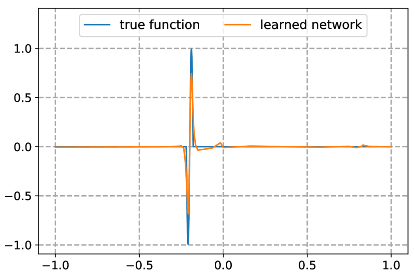
(c) Epoch 2000.

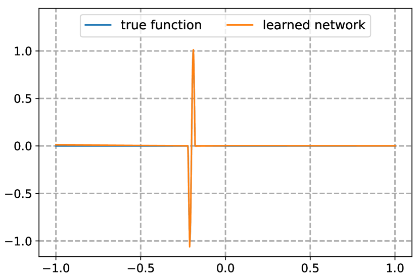
(d) Epoch 20000.

Figure 12: Illustrations of the training process.

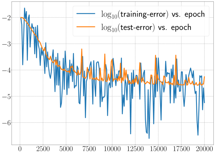
Figure 13: Training and test errors measured in MSE vs. epoch.

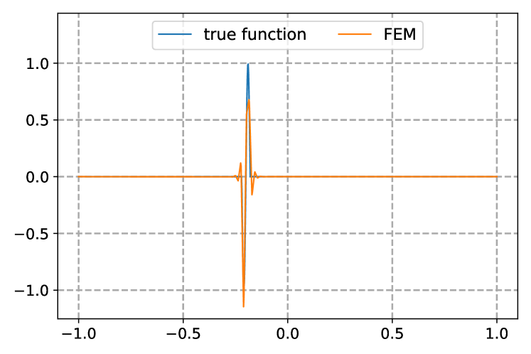
(a) FEM.

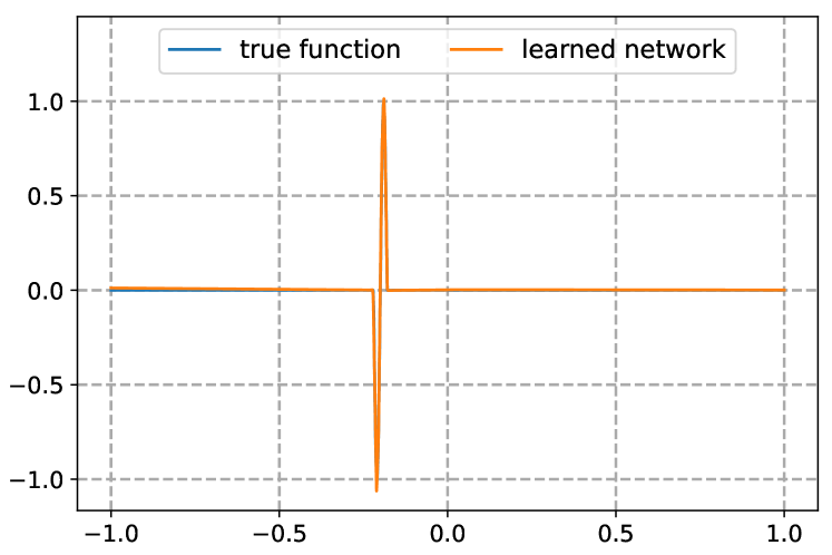
(b) MMNN.

Figure 14: (a) Least square using equally spaced 153 FEM bases. (b) MMNN with $(16+1)\times 4\times(3-1)+(16+1)=153$ free parameters.

Now we show an example in 2D shown in Figure 16 and defined in polar coordinates by

$$f(r,\theta)=\begin{cases}0&\textnormal{if }0.5+25\rho-25r\leq 0,\\ 1&\textnormal{if }0.5+25\rho-25r\geq 1,\\ 0.5+25\rho-25r&\textnormal{otherwise},\\ \end{cases}\quad\textnormal{where}\quad\rho=0.1+0.02\cos(8\pi\theta).$$

Again a rather compact MMNN of size $(100,10,6)$ can produce a good approximation. Figure 17 shows the error during the training process and Figure 16 shows the $\log$ plot of training and testing errors in MSE. For this test there are a total of $400^{2}$ uniformly sampled points in $[-1,1]^{2}$ with mini-batch size of $1000$ and a learning rate of $10^{-3}\times 0.9^{\lfloor k/25\rfloor}$, where $k=1,2,\mathinner{\mkern-0.1mu\cdotp\mkern-0.3mu\cdotp\mkern-0.3mu\cdotp\mkern-0.1mu},1000$ is the epoch number. We compare the result with piecewise linear interpolation and least square approximation using FEM basis on a uniform grid with the same number of degrees of freedom in Figure 18. As observed before, MMNN renders the best result due to its adaptivity through training.

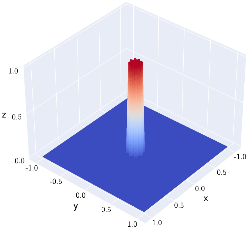
Figure 15: Target function.

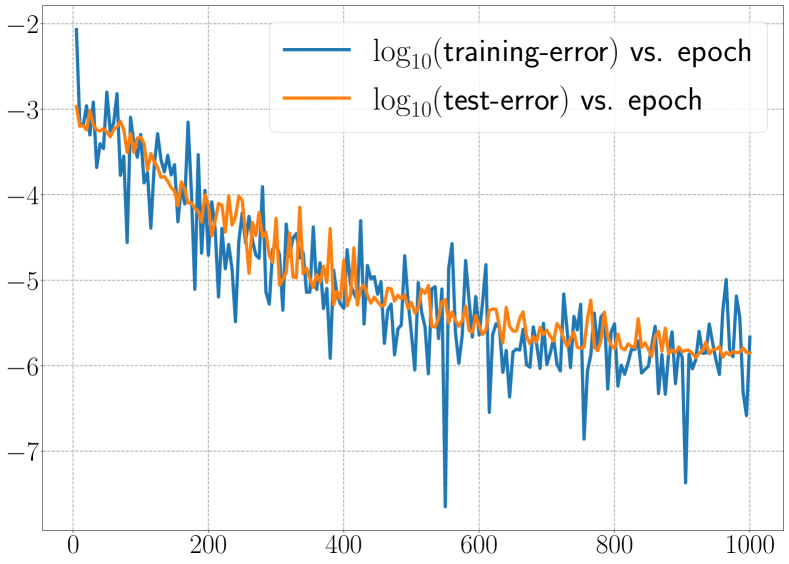
Figure 16: Training and test errors measured in MSE.

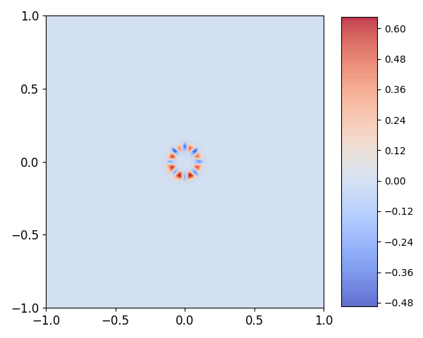
(a) Epoch 10.

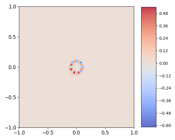
(b) Epoch 50.

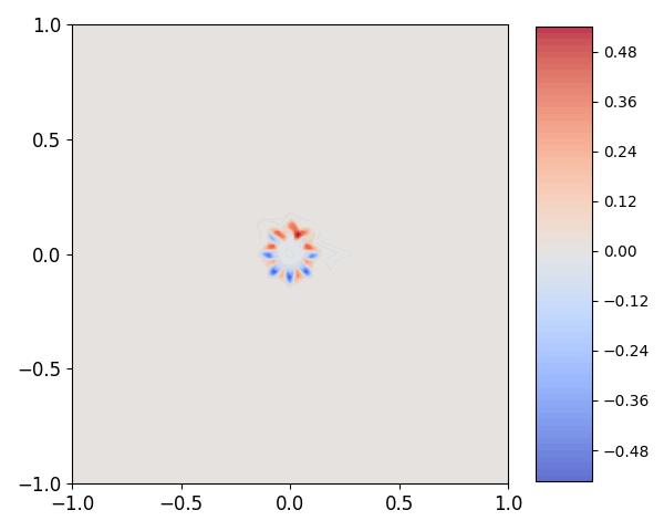
(c) Epoch 100.

(d) Epoch 1000.

Figure 17: The error during the training process.

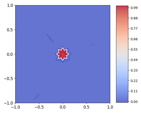
(a) Network.

(b) Interpolation.

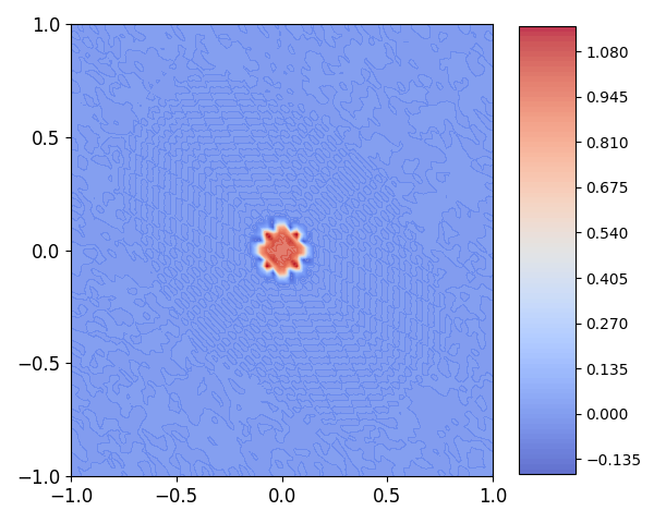
(c) FEM.

(d) Network (difference).

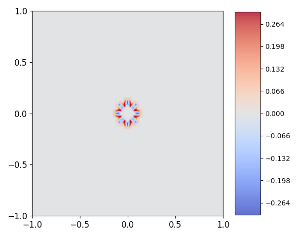
(e) Interpolation (difference).

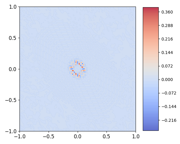
(f) FEM (difference).

Figure 18: Comparison among different approximations using MMNN, interpolation, and least square FEM. The interpolation and FEM are all based on a $72\times 72=5184$ uniform grid. MMNN has $(100+1)\times 10\times(6-1)+(100+1)=5151$ free parameters. The maximum error is approximately $0.05$ for MMNN, $0.31$ for interpolation, and $0.38$ for FEM. The corresponding MSE errors are $0.85\times 10^{-6}$, $1.95\times 10^{-4}$, and $1.45\times 10^{-4}$, respectively.

4.2 Highly oscillatory functions

Globally oscillatory functions with significant high-frequency components can not be approximated well by a shallow network when a global bounded activation function of the form $\sigma({\bm{W}}\cdot{\bm{x}}-{\bm{b}})$, such as ReLU, is used. Due to almost orthogonality or high decorrelation (in terms of the inner product) between $\sigma({\bm{W}}\cdot{\bm{x}}-{\bm{b}})$ and oscillatory functions with high likelihood (in terms of a random choice of $({\bm{W}},{\bm{b}})$), the set of parameters that can render a good approximation, namely the Rashomon set [29], becomes smaller and smaller (in terms of relative measure) and hence harder and harder to find as the target function becomes more and more oscillatory (see [38]). Although this difficulty can be alleviated by complexity decomposition using MMNN as shown in Section 2, it still requires a larger network in terms of width, rank, and layers and more training. Here we limit our tests to oscillatory functions in 1D and 2D due to the dramatic increase of complexity with dimensions, or the curse of dimensions, in general.

We again start with a 1D example, $f(x)=\sin(50\pi x),x\in[-1,1]$. A MMNN of size $(800,40,15)$ produces a good approximation of this highly oscillatory function, as illustrated by the error plot in Figure 20, with a smaller learning rate and a longer training process compared to previous examples with localized fine features. Due to the significant depth, we consider using ResMMNN as discussed in Section 2.2. For this test, a total of $1000$ uniformly sampled points in $[-1,1]$ are used with a mini-batch size of $100$ and a learning rate of $10^{-4}\times 0.9^{\lfloor k/800\rfloor}$, where $k=1,2,\mathinner{\mkern-0.1mu\cdotp\mkern-0.3mu\cdotp\mkern-0.3mu\cdotp\mkern-0.1mu},40000$ is the epoch number. Also, an interesting learning dynamics for Adam is observed from Figure 20. In the beginning, nothing seems to happen until about epoch 3600 when learning starts from the boundary. Then more and more features are captured from the boundary to the inside gradually. Eventually, all features are captured and then fine-tuned together to improve the overall approximation.

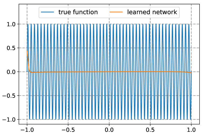
(a) Epoch 3600.

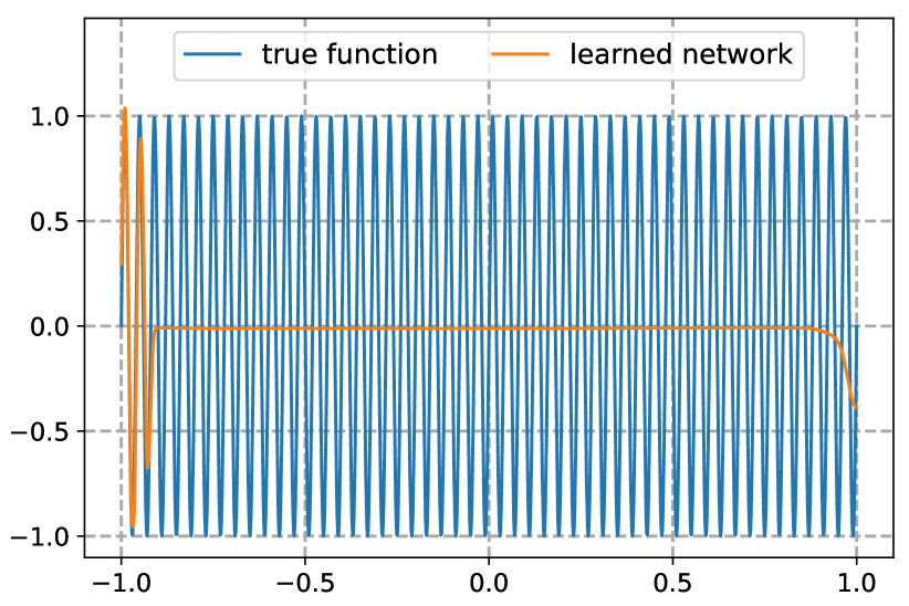
(b) Epoch 3800.

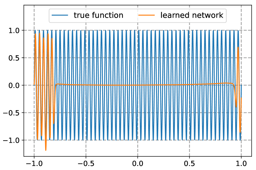
(c) Epoch 4200.

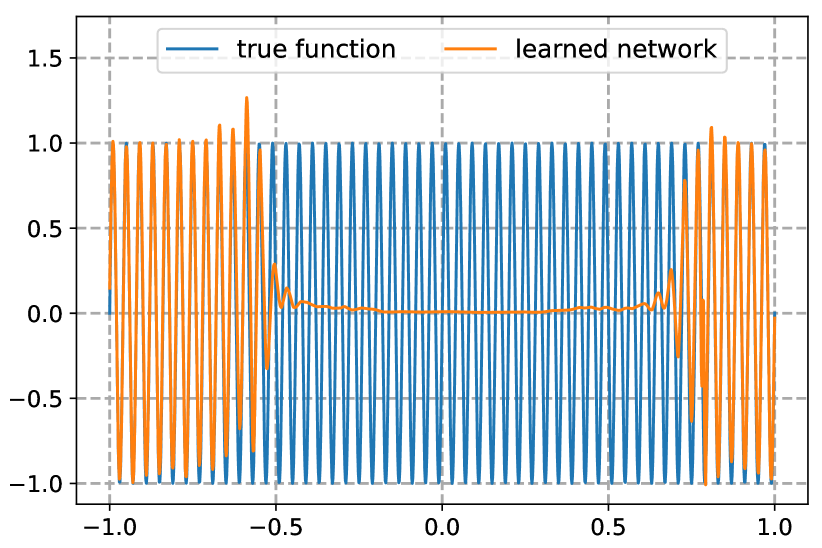
(d) Epoch 5000.

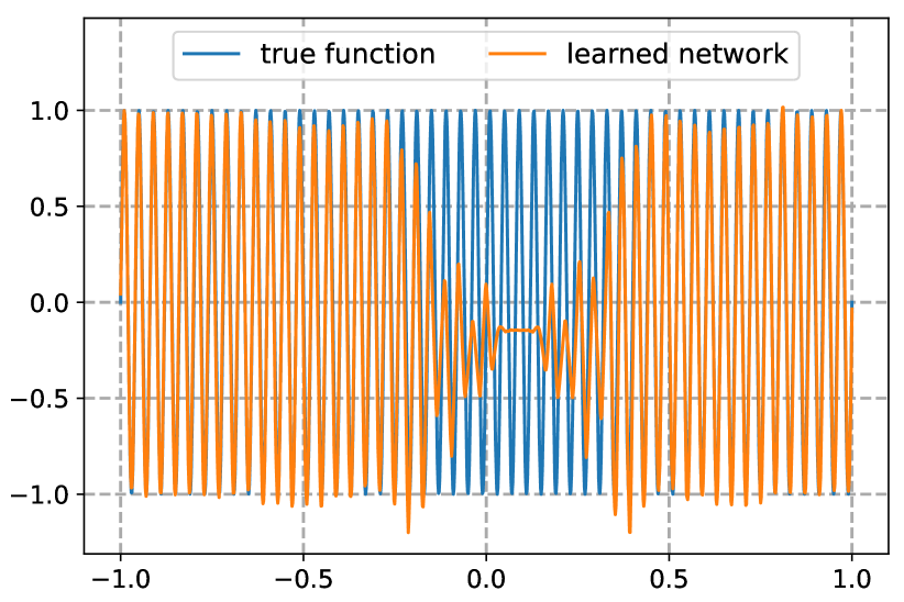
(e) Epoch 10000.

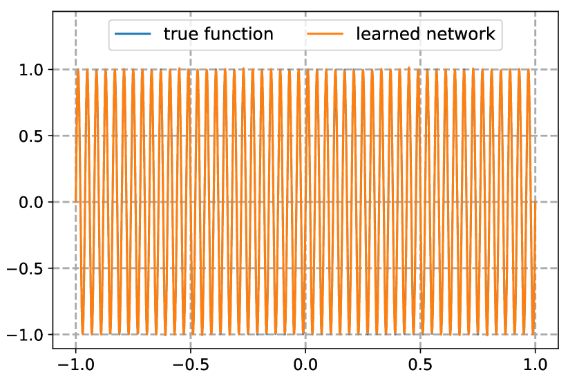
(f) Epoch 40000.

Figure 19: Illustrations of the training process.

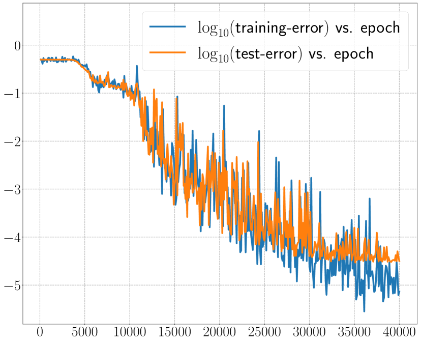
Figure 20: Illustrations of training and test errors measured in MSE.

Next, we consider a two-dimensional target function of the following form:

$$f_{s}(x_{1},x_{2})=\sum_{i=1}^{2}\sum_{j=1}^{2}a_{ij}\sin(sb_{i}x_{i}+sc_{ij}x_{i}x_{j})\cos(sb_{j}x_{j}+sd_{ij}x_{i}^{2}),$$

where

$$(a_{i,j})=\begin{bmatrix}0.3&0.2\\ 0.2&0.3\end{bmatrix},\qquad(b_{i})=\begin{bmatrix}2\pi\\ 4\pi\end{bmatrix},\qquad(c_{i,j})=\begin{bmatrix}2\pi&4\pi\\ 8\pi&4\pi\end{bmatrix},\quad\textnormal{and}\quad(d_{i,j})=\begin{bmatrix}4\pi&6\pi\\ 8\pi&6\pi\end{bmatrix}.$$

In our test, we choose $s=3$ to ensure the function exhibits significant oscillations and contains diverse Fourier modes as illustrated by Figure 22. Given the complexity of the function, we employ a MMNN with size $(600,30,15)$. Again, ResMMNN is used due to the depth. For this test, a total of $400^{2}$ data are sampled on a uniform grid in $[-1,1]^{2}$ with a mini-batch size of $1000$ and a learning rate of $10^{-3}\times 0.9^{\lfloor k/40\rfloor}$, where $k=1,2,\mathinner{\mkern-0.1mu\cdotp\mkern-0.3mu\cdotp\mkern-0.3mu\cdotp\mkern-0.1mu},2000$ is the epoch number. The training process is illustrated by Figure 23. Figure 22 shows $\log$-error plot.

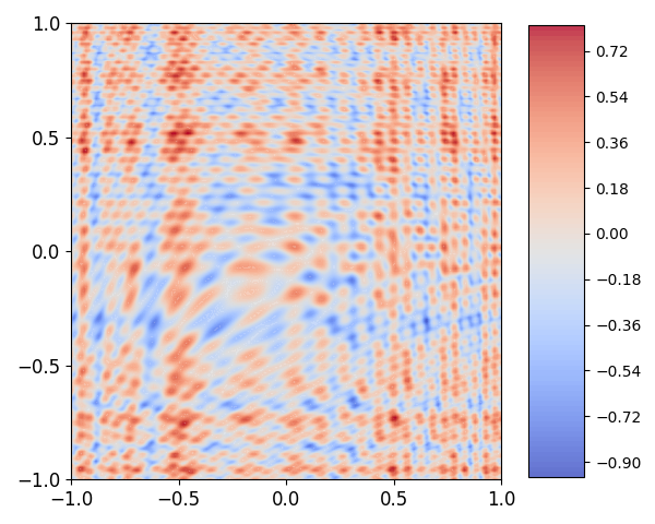
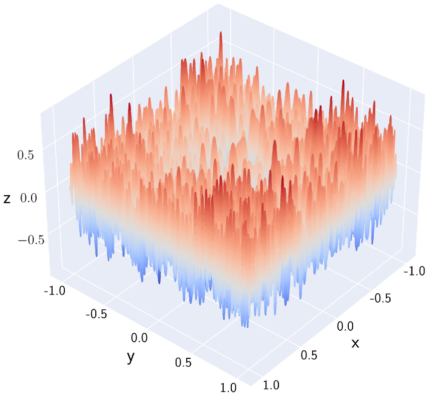
Figure 21: Illustrations of the target function.

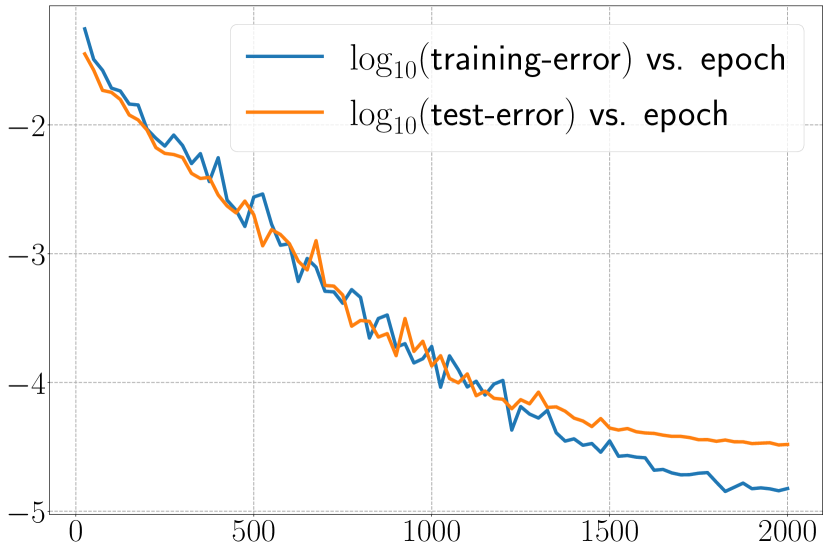
Figure 22: Training and test errors measured in MSE.

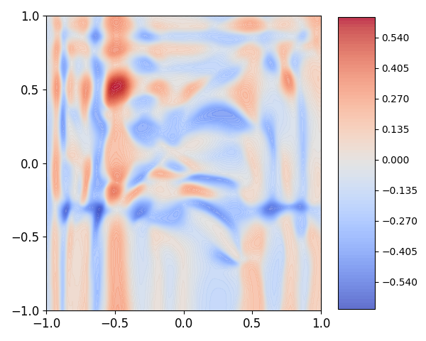
(a) Epoch 25.

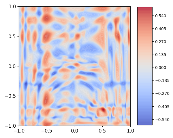
(b) Epoch 50.

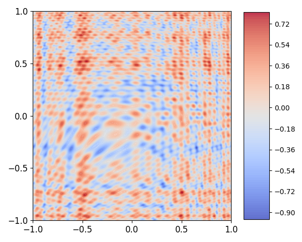
(c) Epoch 1000.

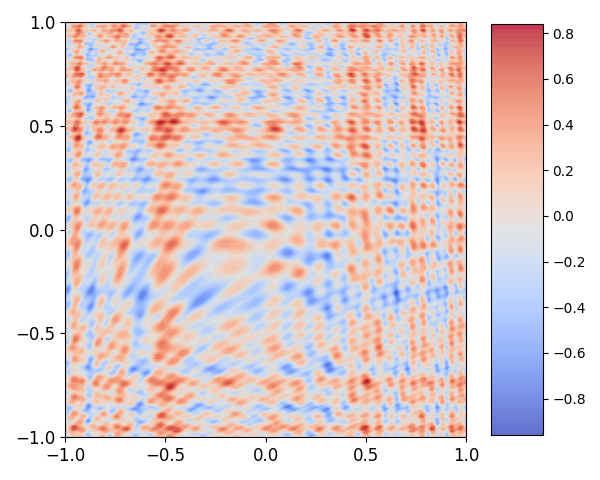
(d) Epoch 2000.

(e) Epoch 25.

(f) Epoch 50.

(g) Epoch 1000.

(h) Epoch 2000.

Figure 23: The top row: the learned neural network; the bottom row: the differences between the learned neural network and the target function.

We trained the same function using identical network settings, except we limited the domain of interest to a unit disc. We sampled $452^{2}$ data points uniformly distributed over the $[-1,1]^{2}$ area, then filtered to retain only those points that fall within the unit disk, totaling approximately $159692$ $(\approx 400^{2})$ samples. As illustrated in Figure 24, our network successfully learned the target function in the disc with no adjustments or modifications. This test highlights the network’s flexibility for domain geometry, an advantage over traditional mesh or grid-based methods, especially in higher dimensions.

(a) Approximation by MMNN.

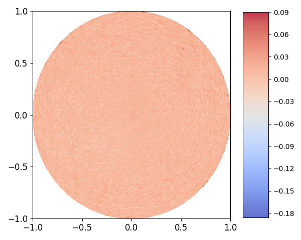
(b) Difference.

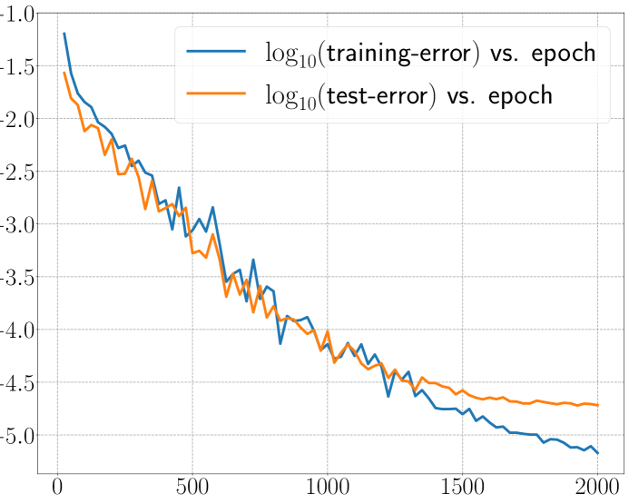
(c) Errors (in MSE) vs. epoch

Figure 24: Approximation in a unit disk.

4.3 Tests in three dimension and higher

In this section, we test a few examples in three and four dimensions. Even sampling an interesting function becomes challenging as the dimension becomes higher. Although our examples are limited by our computation power using a laptop, our tests show that MMNN performs well and is more effective than a fully connected network.

The first example is a 3D function a level set of which is shown in Figure 27. Using polar coordinates $(r,\theta,\phi)$, $\theta\in[0,\pi]$, $\phi\in[0,2\pi)$, the target function $f(x,y,z)$ is defined as:

$$f(r,\theta,\phi)=\begin{cases}0&\text{if }0.5+5\rho-5r\leq 0,\\ 1&\text{if }0.5+5\rho-5r\geq 1,\\ 0.5+5\rho-5r&\text{otherwise},\end{cases}$$

where

$$\rho=\rho(\theta,\phi)=0.5+0.2\sin(6\theta)\cos(6\phi)\sin^{2}(\theta).$$

Figure 25: Surface plot of the levelset $f(r,\theta,\phi)=0.5$.

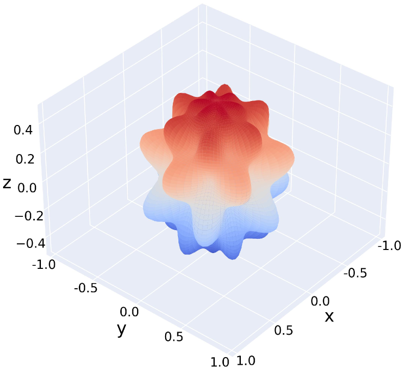
Figure 26: Surface plot of the levelset $h(r,\theta,\phi)=0.5$.

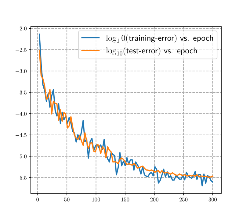
Figure 27: Training and test errors (MSE) vs. epoch.

Our MMNN is of a compact size $(600,20,8)$. For this test, a total of $111^{3}$ data are sampled on a uniform grid in $[-1,1]^{3}$ with a mini-batch size of $999$ and a learning rate of $0.0005\times 0.9^{\lfloor k/6\rfloor}$ for epochs $k=1,2,\mathinner{\mkern-0.1mu\cdotp\mkern-0.3mu\cdotp\mkern-0.3mu\cdotp\mkern-0.1mu},300$. Figure 27 gives the error plot. As shown in Figures 27 and 27, the levelsets corresponding to the target function $f$ and the learned MMNN approximation $h$ are nearly identical. To visually demonstrate the quality of the approximation and complex structure of the 3D function, we present several slices of the target function and the MMNN approximation by fixing either $x$, $y$, or $z$ in Figure 28.

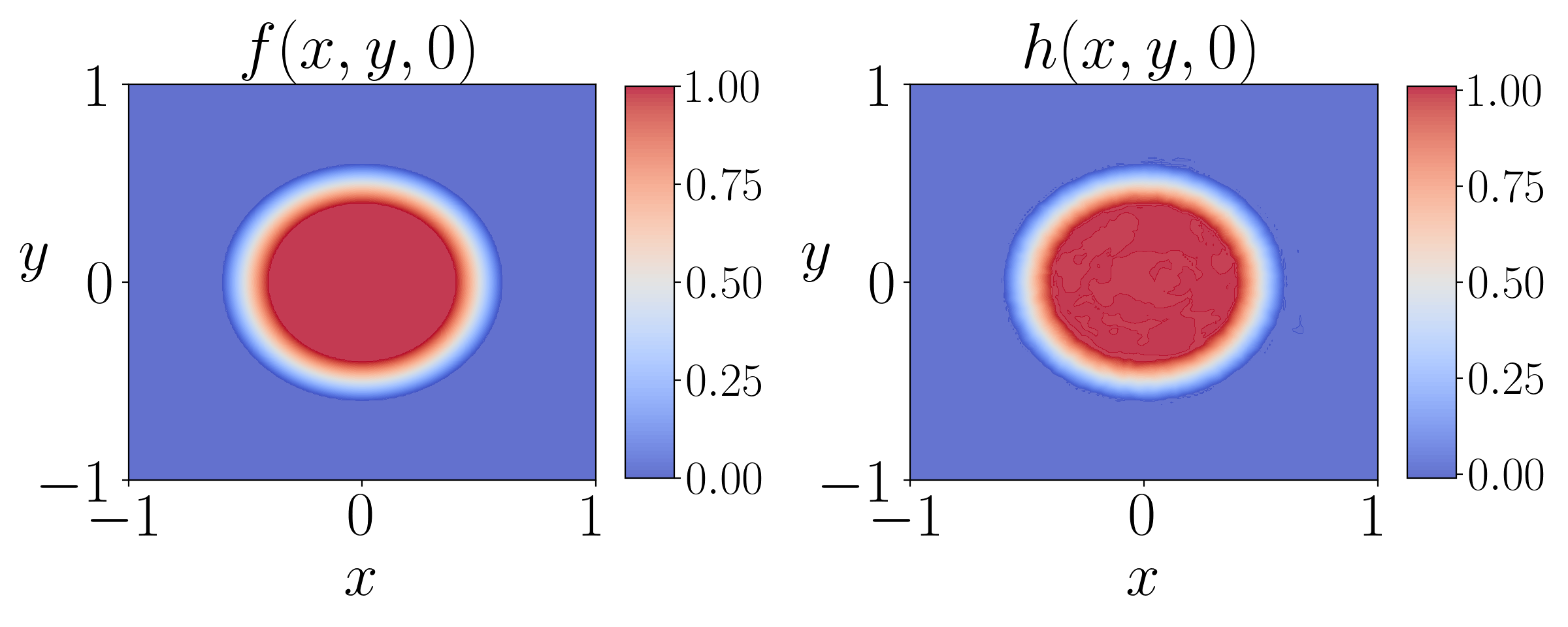
(a) $z=0$.

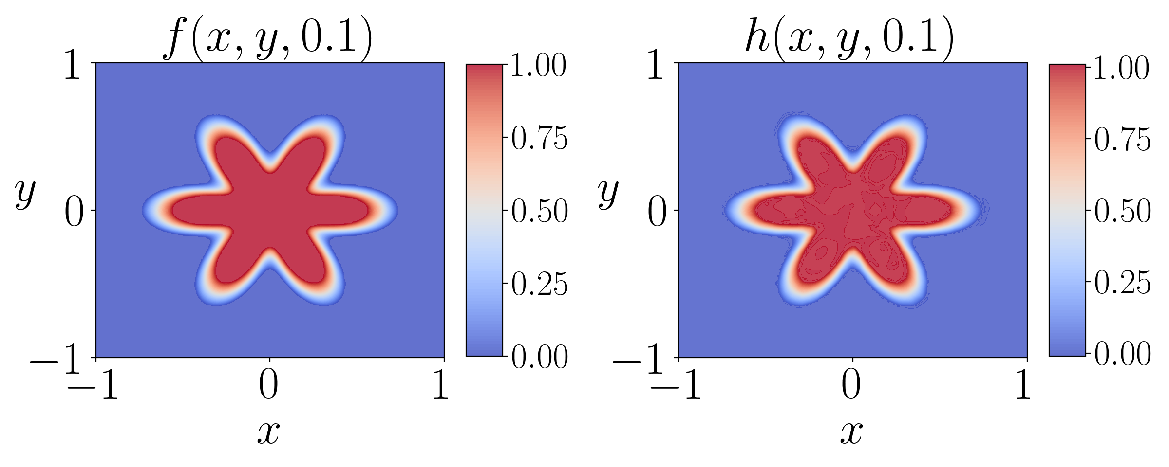
(b) $z=0.1$.

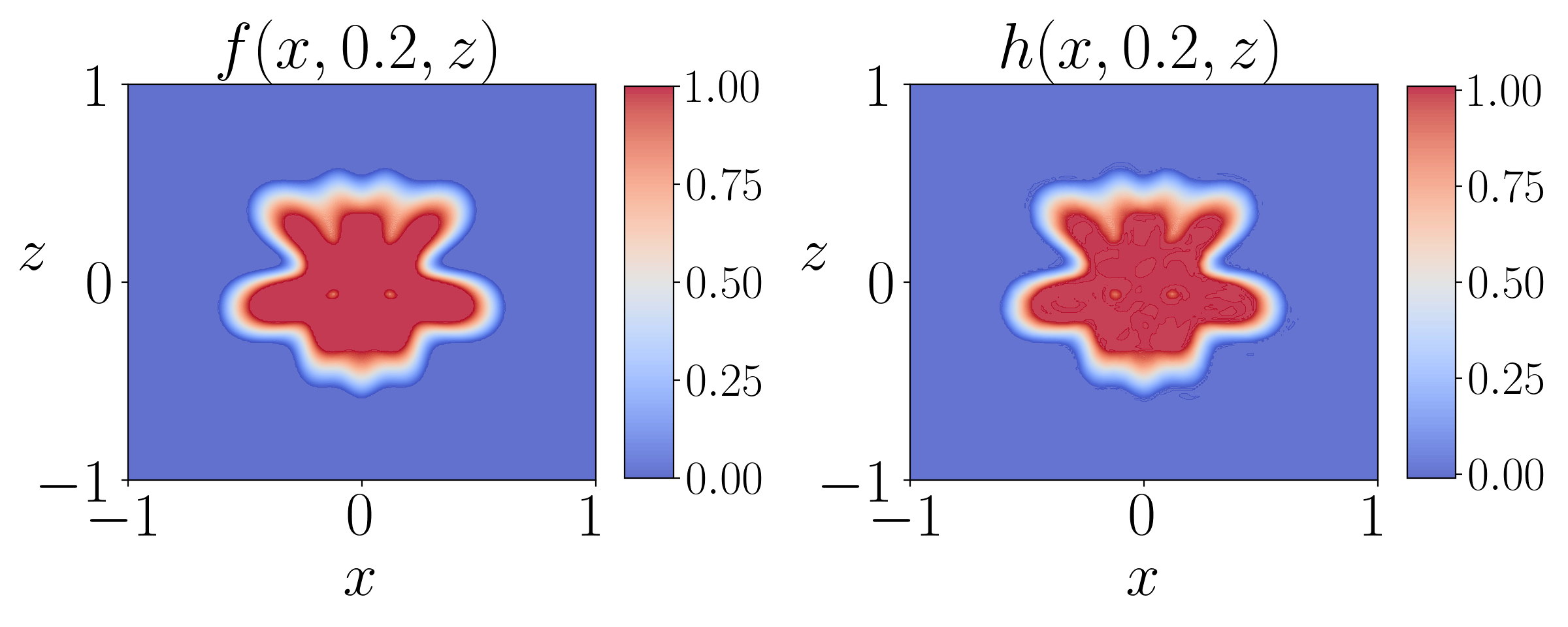
(c) $y=0.2$.

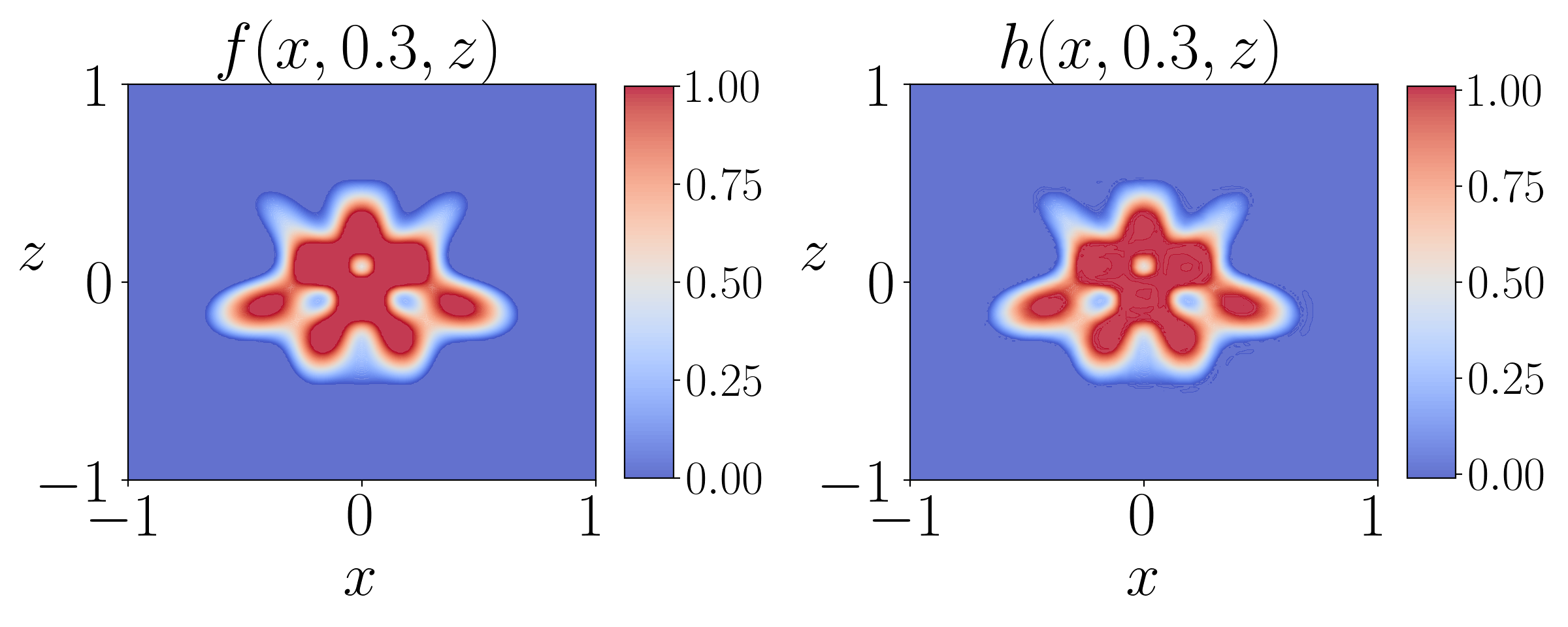
(d) $y=0.3$.

(e) $x=0.4$.

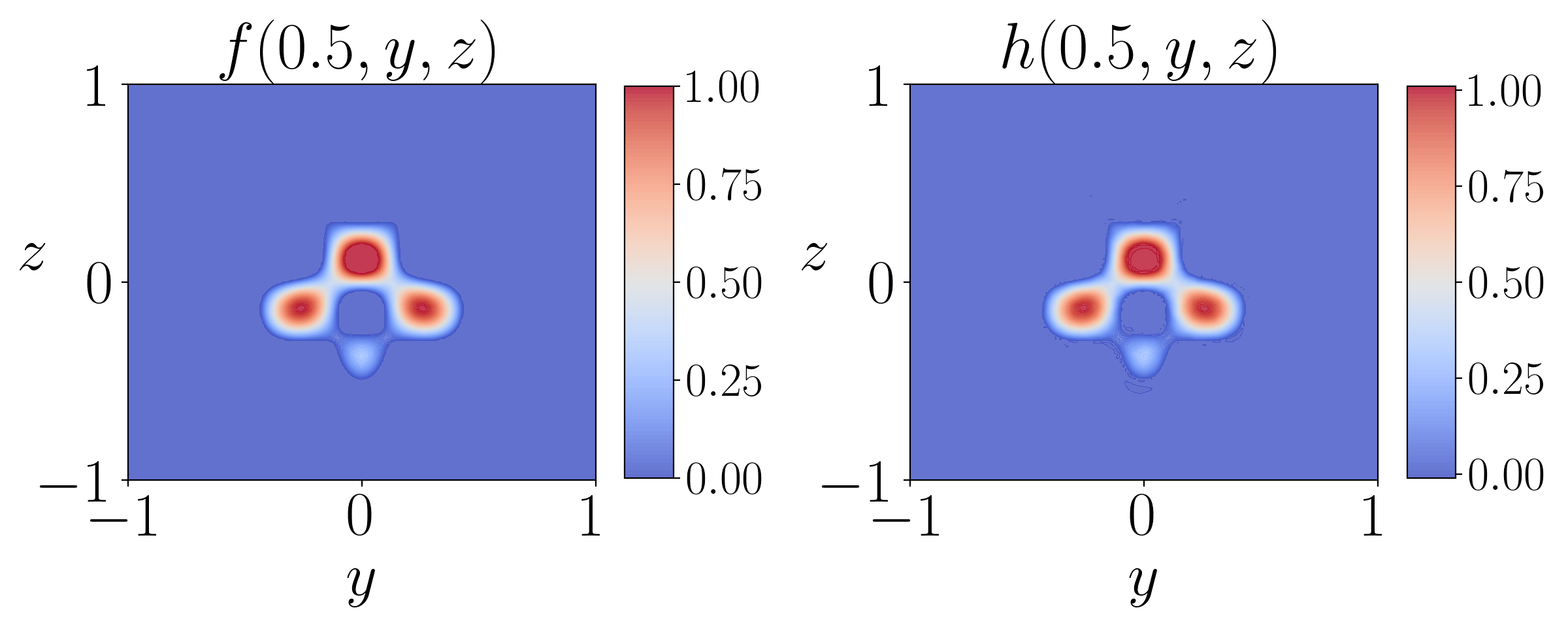
(f) $x=0.5$.

Figure 28: Slices of the true function $f(x,y,z)$ vs. those of the MMNN approximation $h(x,y,z)$.

Next, we consider the probability density function (PDF) of a Gaussian (normal) distribution in 4D,

$$f(\bm{x})=f(x_{1},\dots,x_{4})=\frac{\exp\left(-\frac{1}{2}(\bm{x}-\bm{\mu})^{\textsf{T}}{\bm{\Sigma}}^{-1}(\bm{x}-\bm{\mu})\right)}{\sqrt{(2\pi)^{k}\det({\bm{\Sigma}})}}$$

where ${\bm{\Sigma}}$ is the covariance matrix. We set $\bm{\mu}=\bm{0}$ and ${\bm{\Sigma}}^{-1}=20\left[\begin{smallmatrix}1.0&0.9&0.8&0.7\\ 0.9&2.0&1.9&1.8\\ 0.8&1.9&3.0&2.9\\ 0.7&1.8&2.9&4.0\\ \end{smallmatrix}\right].$ We remark that the eigenvalues of ${\bm{\Sigma}}^{-1}$ are $6.82,9.93,25.28,158.05$ which means that the distribution is quite anisotropic and concentrated near the center.

A compact MMNN with size of $(500,12,6)$ produces a good approximation as shown in the error plot Figure 30. Figure 30 compares the true function $f(x,y,z,u)$ and the MMNN approximation $h(x,y,z,u)$ with $z=u=0.2$. For this test a total of $35^{4}$ data are sampled on a uniform grid in $[-1,1]^{4}$ with a mini-batch size of $35^{2}$ and a learning rate at $10^{-3}\times 0.9^{\lfloor k/6\rfloor}$ for epochs $k=1,2,\mathinner{\mkern-0.1mu\cdotp\mkern-0.3mu\cdotp\mkern-0.3mu\cdotp\mkern-0.1mu},300$.

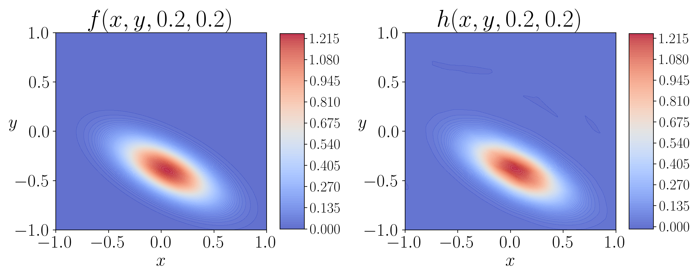
Figure 29: True function $f(x,y,z,u)$ versus the learned network $h(x,y,z,u)$ with $z=u=0.2$.

Figure 30: Training and test errors (MSE) vs. epoch.

4.4 Learning dynamics

In this section, we show some interesting learning dynamics observed during the training process. As the first example in Section 4.2 and the following examples show, the training process not just learns from low frequency first but can also learn feature by feature, i.e., can be localized in both frequency domain and spatial domain. We believe this is due to the combination of MMNN’s “divide and conquer” ability and the Adam optimizer which utilizes momentum. More understanding is needed and will be studied in our future research.

We again start with a 1D example, $f(x)=\sin\big{(}36\pi|x|^{1.5}\big{)},x\in[-1,1]$. A MMNN of size $(600,30,8)$ produces a good approximation of this highly oscillatory function, as illustrated by the error plot in Figure 32. For this test, a total of $1000$ uniformly sampled points in $[-1,1]$ are used with a mini-batch size of $100$ and a learning rate of $10^{-3}\times 0.9^{\lfloor k/200\rfloor}$, where $k=1,2,\mathinner{\mkern-0.1mu\cdotp\mkern-0.3mu\cdotp\mkern-0.3mu\cdotp\mkern-0.1mu},10000$ is the epoch number. As illustrated in Figure 32, the function is less oscillatory near 0. Therefore, we might anticipate that the network will initially learn the part near 0 and then feature by feature from the middle to the boundary. The experimental results presented in Figure 33 agree with our expectations.

Figure 31: Derivative of the target function.

Figure 32: Errors (in MSE) vs. epoch.

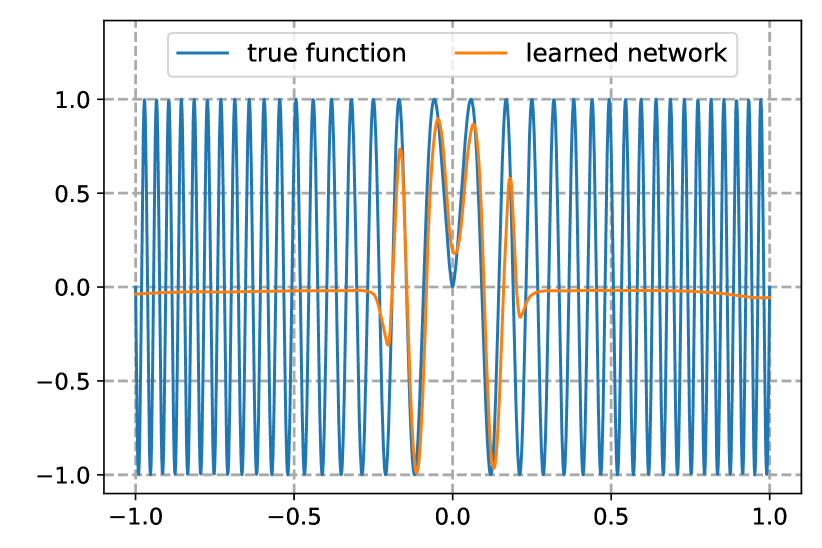
(a) Epoch 400.

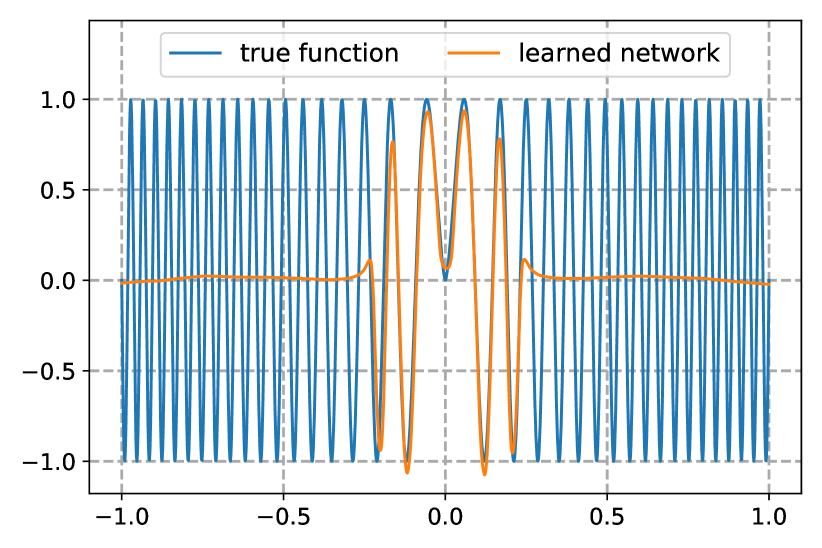
(b) Epoch 500.

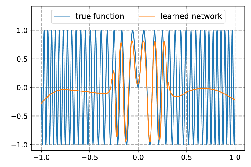
(c) Epoch 600.

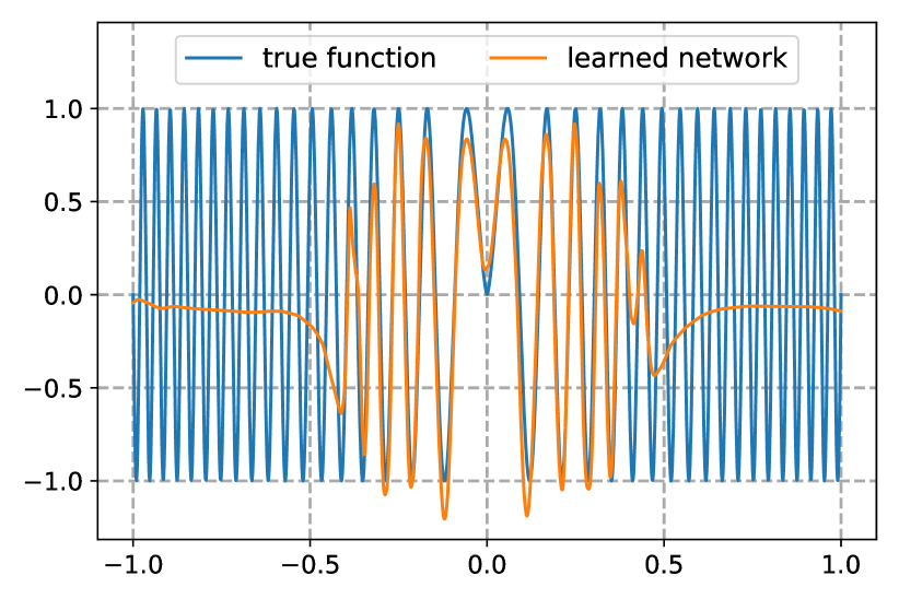
(d) Epoch 700.

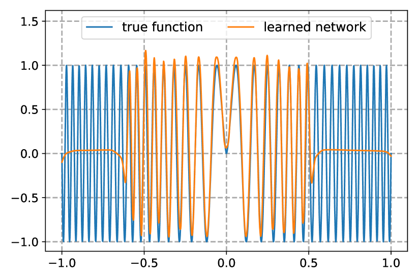
(e) Epoch 1000.

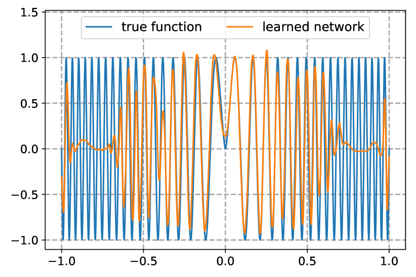
(f) Epoch 1700.

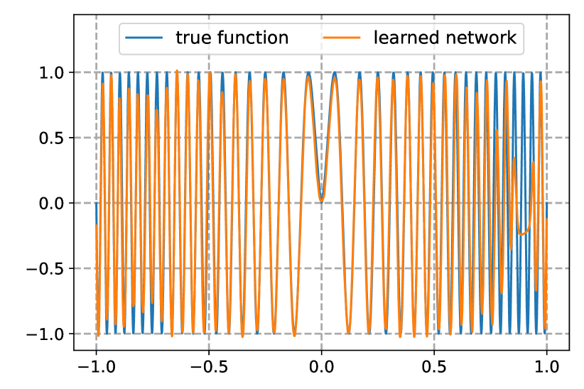
(g) Epoch 2400.

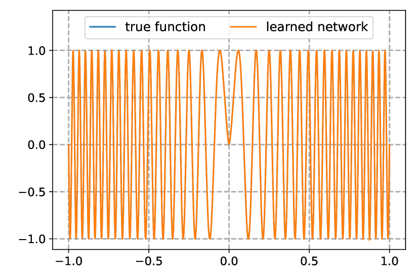
(h) Epoch 10000.

Figure 33: Illustration of the training process.

Now we show an example of 2D function $f(r,\theta)$ (see Figure 35) defined in polar coordinates $(r,\theta)$ as

$$f(r,\theta)=\begin{cases}0&\textnormal{if }0.5+5\rho-5r\leq 0,\\ 1&\textnormal{if }0.5+5\rho-5r\geq 1,\\ 0.5+5\rho-5r&\textnormal{otherwise},\\ \end{cases}\quad\textnormal{where}\quad\rho=0.5+0.1\cos(\pi^{2}\theta^{2}).$$

Our MMNN is of a compact size $(500,20,8)$. For this test, a total of $600^{2}$ data are sampled on a uniform grid in $[-1,1]^{2}$ with a mini-batch size of $1000$ and a learning rate of $0.001\times 0.9^{\lfloor k/6\rfloor}$ for epochs $k=1,2,\mathinner{\mkern-0.1mu\cdotp\mkern-0.3mu\cdotp\mkern-0.3mu\cdotp\mkern-0.1mu},300$. Figure 35 gives the error plot. The training process shown in Figure 36 illustrates that an overall coarse scale or low-frequency component of the shape is learned first and then localized features are learned one by one from coarse to fine.

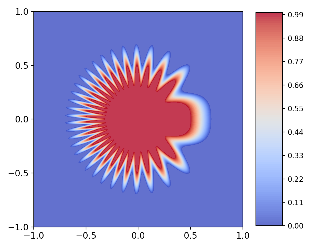
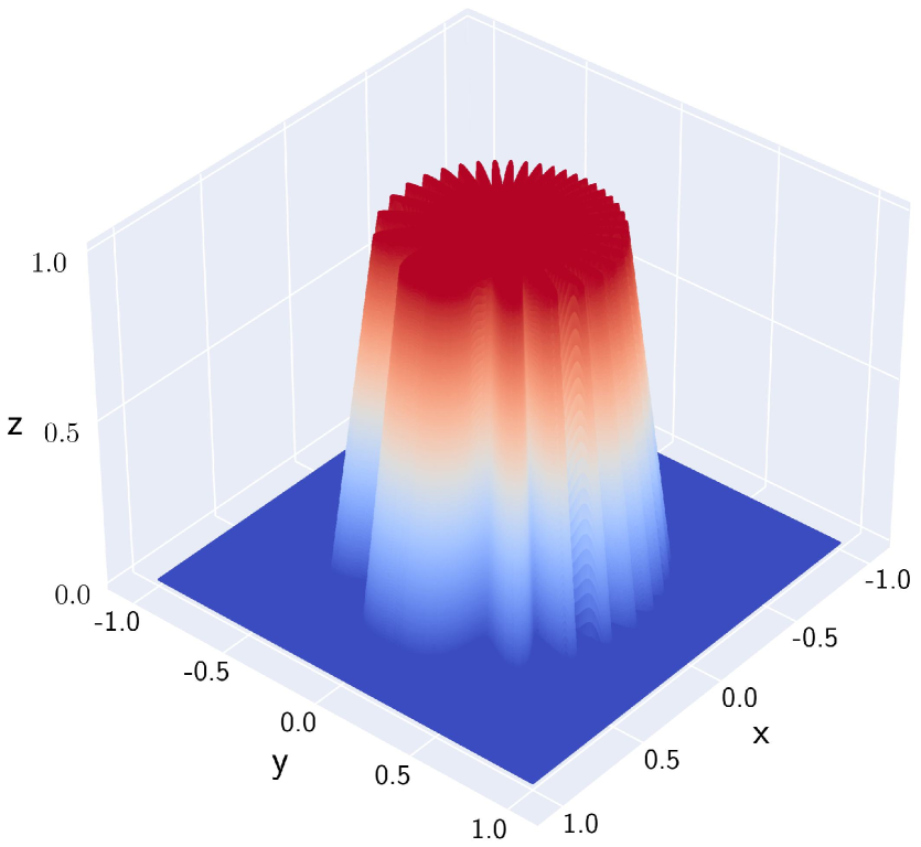
Figure 34: Illustration of the target function.

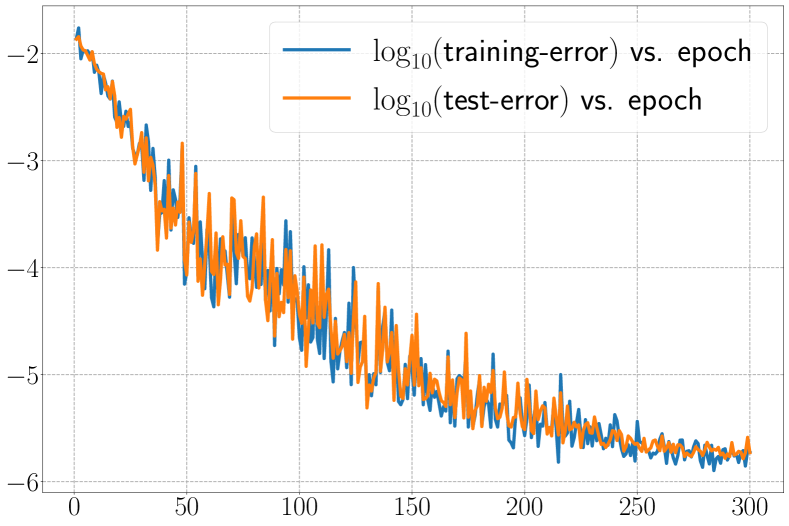
Figure 35: Training and test errors (in MSE) vs. epoch.

(a) Epoch 1.

(b) Epoch 3.

(c) Epoch 5.

(d) Epoch 7.

(e) Epoch 14.

(f) Epoch 22.

(g) Epoch 30.

(h) Epoch 300.

Figure 36: Illustration of the learning dynamics.

5 Further discussion

In this section, we provide several general insights about MMNNs. First, in Section 5.1, we explore the advantages of MMNNs compared to fully connected networks (FCNNs) or multi-layer perceptrons (MLPs). Next, in Section 5.2, we offer practical guidelines for determining the appropriate MMNN size based on our theoretical understanding and extensive numerical experiments. Finally in Section 5.3, we discuss the use of alternative activation functions beyond $\mathtt{ReLU}$ in MMNNs.

5.1 Advantages compared to FCNNs or MLPs

• The two key differences between a standard FCNN or MLP and a MMNN are 1) the introduction of the weights ${\bm{A}},{\bm{c}}$ for different linear combinations of hidden neurons (or perceptrons) as the multi-components in each layer, and 2) the training strategy that fixes those randomly initialized ${\bm{W}},{\bm{b}}$ (random features) in the hidden neurons. Hence it is extremely easy to modify a FCNN or MLP to a MMNN.

• MMNNs are much more effective than FCNNs in terms of representation, training, and accuracy especially for complex functions. In comparison, as shown in those experiments in Section 2.4, MMNNs 1) have much fewer training parameters, 2) converge much faster in training, 3) achieve much better accuracy. Moreover, experiments show that training process of MMNNs converges not only faster but also with a steady rate while FCNNs saturates pretty early to a quite low accuracy, as commonly observed in practices. These nice behaviors of MMNNs are due to their balanced structure for smooth decomposition as well as the training strategy. In practice, the introduction of ${\bm{A}},{\bm{c}}$ in MMNNs provides an important balance between the network width, which is the number of hidden neurons (basis functions) and can be very large, and the dimension of the input space, which is the number of components from the previous layer and can be much smaller than the network width. In other words, using a few linear combinations of the basis functions can capture smooth structures in the input space well. On the other hand, for FCNNs the two are the same and no balance is exerted.

5.2 Practical guidelines for MMNN

There are three hyperparameters for the configuration of MMNN sizes, the network width, the number of components (rank), and the number of layers (depth). Here are the general guidelines based on our mathematical construction and extensive experiments:

1. The network width should provide enough resolution to capture fine details of the target function. This means that the width should be at least comparable to the size of an adaptive mesh that can approximate the target function well.

2. The number of components (rank) is related to the overall complexity of the target function which depends on its spatial domain and Fourier domain representation as well as the input dimension. As indicated by our mathematical multi-component construction, it is related to the “divide and conquer” strategy.

3. The number of layers (depth) is also related to the overall complexity of the target function as for the number of components. Rank and depth are complementary but work together effectively for a smooth decomposition of the target function. The rule of thumb for depth is similar to that for the rank.

Here we use more concrete examples to illustrate the guidelines. For simplicity we fix the input dimension and domain of interest. As the domain size and dimension increases, the network size needs to increase correspondingly. For a smooth target function, a compact MMNN in terms of width, rank, and depth is enough and easy training process can render accurate results. Larger MMNNs are needed for target functions with localized rapid changes. Even with a relative compact size, the training process can allocate resources adaptive to the target function and render good approximation. The most difficult situation is to approximate globally highly oscillatory functions with diverse Fourier modes for which large MMNNs are needed. For instance, if the oscillation frequency doubles, the network width should increase by $2^{d}$ where $d$ is the dimension. In general the network width needs to deal with the curse of dimensionality just like a mesh based method. However, the growth of the number of components and layers with the increase of complexity seems to be relative mild (maybe polylogarithmic suggested by our mathematical construction).

• Overall, for a given target function, MMNNs can work well with quite a large range of configuration with a trade-off between the network size and training process. For example, the training process for a network more on the compact size with respect to the complexity of a given target function may become more subtle and challenging, e.g., choosing the appropriate learning rate and batch size, due to the lack of flexibility (or redundancy) of the representation. On the other hand, a network of too large size (or redundancy) with respect to the complexity of a given target function requires unnecessarily expensive training cost. An interesting and important question for future research is how to develop a posteriori strategy to automatically adjust the network size in practice.

• The most advantageous situation for using MMNNs is when approximating a function in relative high dimension which is mostly smooth except for localized fine features, e.g., a distribution in high dimensions concentrated on a low dimensional manifold. Through training, MMNNs can provide an automatic adaptive approximation of the underlying structure which can be challenging for a traditional mesh based method.

• We would like to remark that learning rate scheduler can be a subtle and important issue for all training process in practice. For all our training process, the Step Learning Rate suffices. However, one could consider using other learning rate schedulers, such as the Cosine Scheduler [18] or the gradual warm-up strategy [5]. Exploring and designing a more efficient learning rate scheduler with some automatic restart mechanism is a potential interesting topic for future work.

5.3 Beyond ReLU to other activation functions

We also tried using different activation functions for MMNNs, e.g., $\mathtt{GELU}$ [9], $\mathtt{Swish}$ [25], $\mathtt{Sigmoid}$, and $\mathtt{Tanh}$. In general, ReLU provides the overall best results for various target functions. However, in situations where a smooth (e.g., $C^{s}$ or real analytic) approximation is needed, one might consider using smooth alternatives to $\mathtt{ReLU}$ such as $\mathtt{GELU}$  or $\mathtt{Swish}$, which generally yield results comparable to $\mathtt{ReLU}$:

• For target functions that are $C^{s}$ or even real analytic (and can be highly oscillatory), such as $f(x)=\cos(36\pi x^{2})-0.6\cos(12\pi x^{2})$, $\mathtt{GELU}$ (or $\mathtt{Swish}$) tends to perform slightly better than $\mathtt{ReLU}$.

• For target functions with non-differentiable points, such as $f(x)={\mathds{1}}_{\{|x|<0.02\}}\cdot\sin(50\pi x)$, $\mathtt{GELU}$ (or $\mathtt{Swish}$) generally performs slightly worse than $\mathtt{ReLU}$.

• The use of $\mathtt{GELU}$ (or $\mathtt{Swish}$) typically results in slightly longer training time compared to $\mathtt{ReLU}$.

Additionally, other popular S-shaped activation functions like $\mathtt{Sigmoid}$ and $\mathtt{Tanh}$ have demonstrated poor performance in our tests, possibly due to the vanishing gradient problem. For highly oscillatory target functions, when using $\mathtt{Sigmoid}$ or $\mathtt{Tanh}$ training errors did not even decrease during the training process.

6 Conclusion

In this work, we introduced the Multi-component and Multi-layer Neural Network (MMNN) and demonstrated its effectiveness in approximating complex functions. By incorporating the principles of structured and balanced decomposition, the MMNN architecture addresses the limitations of shallow networks, particularly in capturing high-frequency components and localized fine features. Our proposed network structure as confirmed by extensive numerical experiments can approximate highly oscillatory functions and functions with rapid transitions efficiently and accurately. Additionally, we highlight the advantages of our training strategy, which optimizes only the linear combination weights of basis functions for each component while keeping the parameters within the activation (basis) functions fixed, leading to a more efficient and stable training process.

The theoretical underpinnings and practical implementations presented in this paper suggest that MMNNs offer a promising direction for constructing neural networks capable of handling complex tasks with fewer parameters and reduced computational overhead. Future research can explore further generalizations and applications of MMNNs, as well as investigate the interplay between representation and optimization in more depth.

References

- [1] Helmut. Bölcskei, Philipp. Grohs, Gitta. Kutyniok, and Philipp. Petersen. Optimal approximation with sparsely connected deep neural networks. SIAM Journal on Mathematics of Data Science, 1(1):8–45, 2019.
- [2] Charles K. Chui, Shao-Bo Lin, and Ding-Xuan Zhou. Construction of neural networks for realization of localized deep learning. Frontiers in Applied Mathematics and Statistics, 4:14, 2018.
- [3] George Cybenko. Approximation by superpositions of a sigmoidal function. Mathematics of Control, Signals, and Systems, 2:303–314, 1989.
- [4] Xavier Glorot and Yoshua Bengio. Understanding the difficulty of training deep feedforward neural networks. In Yee Whye Teh and Mike Titterington, editors, Proceedings of the Thirteenth International Conference on Artificial Intelligence and Statistics, volume 9 of Proceedings of Machine Learning Research, pages 249–256, Chia Laguna Resort, Sardinia, Italy, 13–15 May 2010. PMLR.
- [5] Priya Goyal, Piotr Dollár, Ross Girshick, Pieter Noordhuis, Lukasz Wesolowski, Aapo Kyrola, Andrew Tulloch, Yangqing Jia, and Kaiming He. Accurate, Large Minibatch SGD: Training ImageNet in 1 Hour. arXiv e-prints, page arXiv:1706.02677, June 2017.
- [6] Rémi Gribonval, Gitta Kutyniok, Morten Nielsen, and Felix Voigtlaender. Approximation spaces of deep neural networks. Constructive Approximation, 55:259–367, 2022.
- [7] Ingo Gühring, Gitta Kutyniok, and Philipp Petersen. Error bounds for approximations with deep ReLU neural networks in norms. Analysis and Applications, 18(05):803–859, 2020.
- [8] K. He, X. Zhang, S. Ren, and J. Sun. Deep residual learning for image recognition. In 2016 IEEE Conference on Computer Vision and Pattern Recognition (CVPR), pages 770–778, June 2016.
- [9] Dan Hendrycks and Kevin Gimpel. Gaussian error linear units (GELUs). arXiv e-prints, page arXiv:1606.08415, June 2016.
- [10] Kurt Hornik. Approximation capabilities of multilayer feedforward networks. Neural Networks, 4(2):251–257, 1991.
- [11] Kurt Hornik, Maxwell Stinchcombe, and Halbert White. Multilayer feedforward networks are universal approximators. Neural Networks, 2(5):359–366, 1989.
- [12] Yerlan Idelbayev and Miguel Á. Carreira-Perpiñán. Low-rank compression of neural nets: Learning the rank of each layer. In 2020 IEEE/CVF Conference on Computer Vision and Pattern Recognition (CVPR), pages 8046–8056, 2020.
- [13] Aysu Ismayilova and Vugar E. Ismailov. On the kolmogorov neural networks. Neural Networks, 176:106333, 2024.
- [14] Diederik P. Kingma and Jimmy Ba. Adam: A method for stochastic optimization. In Yoshua Bengio and Yann LeCun, editors, 3rd International Conference on Learning Representations, ICLR 2015, San Diego, CA, USA, May 7-9, 2015, Conference Track Proceedings, 2015.
- [15] A. N. Kolmogorov. On the representation of continuous functions of several variables by superposition of continuous functions of one variable and addition. Dokl. Akad. Nauk SSSR, pages 953–956, 1957.
- [16] Fanghui Liu, Xiaolin Huang, Yudong Chen, and Johan A. K. Suykens. Random features for kernel approximation: A survey on algorithms, theory, and beyond. IEEE Transactions on Pattern Analysis and Machine Intelligence, 44(10):7128–7148, 2022.
- [17] Ziming Liu, Yixuan Wang, Sachin Vaidya, Fabian Ruehle, James Halverson, Marin Soljačić, Thomas Y. Hou, and Max Tegmark. KAN: Kolmogorov-Arnold networks. arXiv e-prints, page arXiv:2404.19756, April 2024.
- [18] Ilya Loshchilov and Frank Hutter. Sgdr: Stochastic gradient descent with warm restarts. In 5th International Conference on Learning Representations, ICLR 2017, Toulon, France, April 24-26, 2017, Conference Track Proceedings, 2017.
- [19] Jianfeng Lu, Zuowei Shen, Haizhao Yang, and Shijun Zhang. Deep network approximation for smooth functions. SIAM Journal on Mathematical Analysis, 53(5):5465–5506, 2021.
- [20] Vitaly Maiorov and Allan Pinkus. Lower bounds for approximation by MLP neural networks. Neurocomputing, 25(1):81–91, 1999.
- [21] Hadrien Montanelli and Haizhao Yang. Error bounds for deep ReLU networks using the Kolmogorov-Arnold superposition theorem. Neural Networks, 129:1–6, 2020.
- [22] Alexander Novikov, Dmitrii Podoprikhin, Anton Osokin, and Dmitry P Vetrov. Tensorizing neural networks. Advances in neural information processing systems, 28, 2015.
- [23] Hao Peng, Nikolaos Pappas, Dani Yogatama, Roy Schwartz, Noah Smith, and Lingpeng Kong. Random feature attention. In International Conference on Learning Representations, 2021.
- [24] Ali Rahimi and Benjamin Recht. Random features for large-scale kernel machines. In J. Platt, D. Koller, Y. Singer, and S. Roweis, editors, Advances in Neural Information Processing Systems, volume 20. Curran Associates, Inc., 2007.
- [25] Prajit Ramachandran, Barret Zoph, and Quoc V. Le. Searching for activation functions. arXiv e-prints, page arXiv:1710.05941, October 2017.
- [26] Siddhartha Rao Kamalakara, Acyr Locatelli, Bharat Venkitesh, Jimmy Ba, Yarin Gal, and Aidan N. Gomez. Exploring low rank training of deep neural networks. arXiv e-prints, page arXiv:2209.13569, September 2022.
- [27] Alessandro Rudi and Lorenzo Rosasco. Generalization properties of learning with random features. In I. Guyon, U. Von Luxburg, S. Bengio, H. Wallach, R. Fergus, S. Vishwanathan, and R. Garnett, editors, Advances in Neural Information Processing Systems, volume 30. Curran Associates, Inc., 2017.
- [28] Tara N. Sainath, Brian Kingsbury, Vikas Sindhwani, Ebru Arisoy, and Bhuvana Ramabhadran. Low-rank matrix factorization for deep neural network training with high-dimensional output targets. In 2013 IEEE International Conference on Acoustics, Speech and Signal Processing, pages 6655–6659, 2013.
- [29] Lesia Semenova, Cynthia Rudin, and Ronald Parr. On the existence of simpler machine learning models. In Proceedings of the 2022 ACM Conference on Fairness, Accountability, and Transparency, pages 1827–1858, 2022.
- [30] Zuowei Shen, Haizhao Yang, and Shijun Zhang. Nonlinear approximation via compositions. Neural Networks, 119:74–84, 2019.
- [31] Zuowei Shen, Haizhao Yang, and Shijun Zhang. Deep network approximation characterized by number of neurons. Communications in Computational Physics, 28(5):1768–1811, 2020.
- [32] Zuowei Shen, Haizhao Yang, and Shijun Zhang. Deep network approximation: Achieving arbitrary accuracy with fixed number of neurons. Journal of Machine Learning Research, 23(276):1–60, 2022.
- [33] Zuowei Shen, Haizhao Yang, and Shijun Zhang. Deep network approximation in terms of intrinsic parameters. In Kamalika Chaudhuri, Stefanie Jegelka, Le Song, Csaba Szepesvari, Gang Niu, and Sivan Sabato, editors, Proceedings of the 39th International Conference on Machine Learning, volume 162 of Proceedings of Machine Learning Research, pages 19909–19934. PMLR, 17–23 Jul 2022.
- [34] Aman Sinha and John C Duchi. Learning kernels with random features. In D. Lee, M. Sugiyama, U. Luxburg, I. Guyon, and R. Garnett, editors, Advances in Neural Information Processing Systems, volume 29. Curran Associates, Inc., 2016.
- [35] Dmitry Yarotsky. Error bounds for approximations with deep ReLU networks. Neural Networks, 94:103–114, 2017.
- [36] Dmitry Yarotsky. Optimal approximation of continuous functions by very deep ReLU networks. In Sébastien Bubeck, Vianney Perchet, and Philippe Rigollet, editors, Proceedings of the 31st Conference On Learning Theory, volume 75 of Proceedings of Machine Learning Research, pages 639–649. PMLR, 06–09 Jul 2018.
- [37] Shijun Zhang. Deep neural network approximation via function compositions. PhD Thesis, National University of Singapore, 2020.
- [38] Shijun Zhang, Hongkai Zhao, Yimin Zhong, and Haomin Zhou. Why shallow networks struggle with approximating and learning high frequency: A numerical study. arXiv e-prints, page arXiv:2306.17301, June 2023.
- [39] Ding-Xuan Zhou. Universality of deep convolutional neural networks. Applied and Computational Harmonic Analysis, 48(2):787–794, 2020.