Physical Layer Deception with Non-Orthogonal Multiplexing

Abstract

Physical layer security (PLS) is a promising technology to secure wireless communications by exploiting the physical properties of the wireless channel. However, the passive nature of PLS creates a significant imbalance between the effort required by eavesdroppers and legitimate users to secure data. To address this imbalance, in this article, we propose a novel framework of physical layer deception (PLD), which combines PLS with deception technologies to actively counteract wiretapping attempts. Combining a two-stage encoder with randomized ciphering and non-orthogonal multiplexing, the PLD approach enables the wireless communication system to proactively counter eavesdroppers with deceptive messages. Relying solely on the superiority of the legitimate channel over the eavesdropping channel, the PLD framework can effectively protect the confidentiality of the transmitted messages, even against eavesdroppers who possess knowledge equivalent to that of the legitimate receiver. We prove the validity of the PLD framework with in-depth analyses and demonstrate its superiority over conventional PLS approaches with comprehensive numerical benchmarks.

I Introduction

Physical layer security (PLS) is gaining prominence within wireless communication, aiming to secure transmissions by leveraging physical channel properties, thus offering a fresh layer of security without relying on traditional cryptographic methods. This technological trend is increasingly pivotal in modern wireless networks [1].

However, future wireless networks are expected to support ultra-reliable and low-latency communications (URLLC) [2], where the transmitted packets usually consist of mission-critical information with small amount of bits, e.g., command signals for the actuator or real-time measurement from sensors. Due to the stringent delay requirement, only a limited number of blocklength is assigned to these packets, which indicates the classic assumption of infinite blocklength no longer holds [3]. The short-packet transmissions operated in the so-called finite blocklength (FBL) regime may still suffer from potential decoding error or potential leakage, even if Bob’s channel is stronger than Eve’s channel. To characterize the PLS performance with FBL codes, the authors in [4] provide the bounds of achievable security rate under a given leakage probability and a given error probability, which offers a more general expression in the FBL regime than the Wyner’s secrecy capacity.

On the other hand, driven by the inherent interference along with the superimposed transmission, the non-orthogonal multiplexing technologies shows the potential to be the new opportunities for enhancing the PLS performance [5]. Leveraging the non-orthogonality of the signals, the communication secrecy can be enhanced by constructively engineering interference in the wiretap channel. In fact, it has been proven from an information-theoretic perspective that transmitting open messages simultaneously with confidential messages can improve overall secrecy performance when using a security-oriented precoder design [6].

Despite the latest advances of PLS offering enhanced passive security, a notable imbalance still remains, as eavesdroppers can attempt to wiretap with barely any risk of exposure, and significantly lower effort compared to the extensive measures taken by the network and legitimate users to secure data. This imbalance necessitates a strategic pivot towards integrating active defense mechanisms, like deception technologies, into the wireless security framework. Deception technologies are designed to mislead and distract potential eavesdroppers by fabricating data or environments, thus protecting genuine data. These technologies can also entice eavesdroppers into revealing themselves, offering a proactive approach to maintaining security integrity [7].

In 2023, we proposed a novel framework of physical layer deception (PLD) [8], which pioneered to combine PLS and deception technologies. The PLD framework enables to deceive eavesdroppers and actively counteract their wiretapping attempts. Leveraging our insights of PLS in the FBL regime, a joint optimization of the encryption coding rate and the power allocation was formulated and solved in [8], to simultaneously achieve high secured reliability and effective deception. Nevertheless, as a preliminary effort, this work is still limited in several aspects. First, it lacks in-depth discussion to the error model of wiretap channels in the presence of deceptive ciphering. Second, the optimization problem is set up with a simple objective function that straightforwardly combines the secrecy performance and the deception performance, which lacks flexibility and adaptability to various practical scenarios. Third, the PLD framework is only discussed on a simple point-to-point communication scenario, without discussion on practical implementation and deployment in multi-access networks.

In this article, we extend our previous work and address the aforementioned limitations. With respect to [8], the main novel contributions of this article are summarized as follows:

1. We detail the system model with the distinguished transmission schemes with both activated and deactivated deceptive ciphering, and provide a comprehensive reception error model of the proposed approach in different scenarios.

2. Instead of simply combining the reception rate and deception rate of both the legitimate user and the eavesdropper into a single objective function, we propose in this article to maximize the effective deception rate, while setting a constraint on the leakage-failure probability (LFP). This new setup allows to flexibly adjust the trade-off between the secrecy performance and the deception performance, and to adapt to various practical scenarios. The analyses to the feasibility and convexity of the optimization problem are correspondingly updated, and the numerical solver design also adapted therewith.

3. Two different solutions of conventional PLS, instead of only one in [8], are provided as benchmarks to evaluate the performance of the PLD framework.

4. We extend the discussion of the PLD framework to various aspects of implementation and deployment in practical use scenarios.

The remaining contents of this article are organized as follows. We begin with a brief review to related literature in Sec. II, then setup the models and optimization problem in Sec. III. Afterwards, we present our analyses to the problem and our approach in Sec. IV, which are later numerically validated and evaluated in Sec. V. Finally, we extend our discussion in Sec. VI regarding various perspectives of practical implementation and deployment of the PLD paradigm, before concluding this article with Sec. VII.

II Related Works

The concept of PLS originates from the seminal work of Wyner [9], which generalizes Shannon’s concept of perfect secrecy [10] into a measurable strong secrecy over wiretap channels. Since then, the secrecy performance of communication systems has been studied over different variants of wiretap channels, including binary symmetric channels [11], degraded additive white Gaussian noise (AWGN) channels [12], fading channels [13], multi-antenna channels [14], broadcast channels [15], multi-access channels [16], interference channels [17], relay channels [18], etc. Thanks to the rich insights gained therefrom, optimization methods have been developed in various perspectives, such as radio resource allocation, beamforming and precoding, antenna/node selection and cooperation, channel coding, etc. [19, 20], to enhance the secrecy performance of communication systems.

To investigate the transmission performance in FBL regime, authors in the landmark work [3] derive a tight bound with the closed-form expression for the decoding error probability. This expression and its first-order approximation are widely adopted to investigate FBL performance, especially with ultra-reliable low-latency communication (URLLC) applications [21, 22, 23]. Following this effort, authors in [24] derive the achievable security rate and its tight bounds for both discrete memoryless and Gaussian wiretap channels. Based on that, abounding works have been done to enhance the PLS performance in FBL regime. For example, the authors in [25] investigate the covertness by keeping the confidential signal below a certain signal-to-noise ratio threshold for the wiretap channel so that Eve can not detect the transmission. In [26], the interplay between reliability and security is studied, where the joint secure-reliability performance is enhanced by allocating the resource of the transmissions. This interplay is further investigated in [27], where the concept of trading reliability for security is proposed to characterize the trade-off between security and reliability in PLS for the short-packet transmissions.

Another emerging cluster of research focuses on the application of non-orthogonal multi-access (NOMA) in PLS. NOMA is a promising technology that allows multiple users to share the same frequency and time resources, which can significantly increase spectral efficiency. Especially for PLS, the interference caused by the superposition signals could be beneficial to improve the security [28, 29]. Therefore, NOMA-based PLS has been shown to provide enhanced security compared to conventional approaches. Nevertheless, such studies are also generally considering long codes, leaving NOMA-PLS in the FBL regime a virgin land of research.

In the field of information security, the principles of deception were firstly introduced and well demonstrated by the infamous practices of social engineering by Mitnick [30]. Later, this concept was transferred by Cheswick [31] and Stoll [32] into defensive applications, which were originally called honeypots and thereafter generalized to a broader spectrum of deception technologies [33]. Over the past three decades, deception technologies have been well developed and widely adopted in information systems, across the four layers of network, system, application, and data. Various solutions have been proposed to mitigate, prevent, or to detect cyber attacks. For a comprehensive review on the state-of-the-art of deception technologies, readers are referred to [33, 34, 35]. On the physical layer of wireless systems, however, deception technologies are still in their infancy. Besides our preliminary work [8] that has been introduced in Sec. I, the inspiration of exploiting physical characteristics of wireless channels to proactively deceiving eavesdroppers with fake information is also seen in the works of [36] and [37]. More specifically, the former work leverages the spatial diversity of multi-input multi-output (MIMO) systems to attract an eavesdropper to gradually approach a trap region where fake messages are received, while the latter designs a generative adversarial network (GAN) to generate specialized waveform that paralyzes the eavesdropper’s recognition model.

III Problem Setup

III-A System Model

We consider a typical wireless eavesdropping scenario. The information source Alice sends messages to the sink Bob over its legitimate channel $h_{\mathrm{Bob}}$ with gain $z_{\mathrm{Bob}}=\left|h_{\mathrm{Bob}}\right|^{2}$. Meanwhile, an attacker Eve listens to Alice over the eavesdropping channel $h_{\mathrm{Eve}}$ with gain $z_{\mathrm{Eve}}=\left|h_{\mathrm{Eve}}\right|^{2}$. Though Eve may occur at any position, practically, due to the concern of exposure, she is unlikely staying consistently close to Alice or Bob. In this context, with proper beamforming, Alice is capable of keeping $h_{\mathrm{Bob}}$ statistically superior to $h_{\mathrm{Eve}}$, which allows to apply PLS approaches. To enable physical layer deception, Alice deploys a two-stage encoder followed by non-orthogonal multiplexing (NOM)-based waveforming, as illustrated in Fig. 1.

(a)

(b)

Figure 1: The transmitting scheme of Alice, with deceptive ciphering 1(a) activated and 1(b) deactivated, respectively.

The first stage of the encoder is a symmetric key cipherer that can be optionally activated/deactivated. When activated, as illustrated in Fig. 1(a), it encrypts every $d_{\mathrm{P}}$-bit plaintext message $p$ with an individually and randomly selected $d_{\mathrm{K}}$-bit key $k$ into a $d_{\mathrm{M}}$-bit ciphertext

$$m=f(p,k)\in\mathbb{M},\quad\forall(p,k)\in\left(\mathbb{P}\times\mathbb{K}\right),$$ (1)

where $\mathbb{M}\subseteq\{0,1\}^{d_{\mathrm{M}}}$, $\mathbb{P}\subseteq\{0,1\}^{d_{\mathrm{P}}}$, and $\mathbb{K}\subseteq\{0,1\}^{d_{\mathrm{K}}}$ are the feasible sets of ciphertext codes, plaintext codes, and keys, respectively. On the other hand, given the chosen key $k$, the plaintext can be decrypted from the ciphertext through

$$p=f^{-1}(m,k).$$ (2)

Especially, the codebooks shall be designed to ensure that

$$\mathbb{M}\subseteq\mathbb{P},$$ (3)

and that $\forall\left(m,k,k^{\prime}\right)\in\left(\mathbb{M}\times\mathbb{K}^{2}\right)$ it holds

$$f^{-1}(m,k^{\prime})\left|{}_{k^{\prime}\neq k}\neq f^{-1}(m,k).\right.$$ (4)

The second stage of the encoder is a pair of channel coders, $c_{\mathrm{M}}$ and $c_{\mathrm{K}}$, which attach error correction redundancies to the ciphertext $m$ and the key $k$, respectively. The two output codewords, both $n$ bits long, are then individually modulated before non-orthogonally multiplexed in the power domain:

$$s=\frac{P_{\mathrm{M}}s_{\mathrm{M}}+P_{\mathrm{K}}s_{\mathrm{K}}}{P_{\mathrm{M}}+P_{\mathrm{K}}},$$ (5)

where $s$ is the power-normalized baseband signal to transmit, $s_{\mathrm{M}}$ and $s_{\mathrm{K}}$ the power-normalized baseband signals carrying the ciphertext and the key, respectively. $P_{\mathrm{M}}$, $P_{\mathrm{K}}$, and $P_{\mathrm{M}}+P_{\mathrm{K}}$ are the transmission powers allocated to $s_{\mathrm{M}}$, $s_{\mathrm{K}}$, and $s$, respectively. Particularly, we set $s_{\mathrm{M}}$ as the primary component of the message, and $s_{\mathrm{K}}$ the secondary, so that $P_{\mathrm{M}}>P_{\mathrm{K}}$. On the receiver side, for both $i\in\{\text{Bob},\text{Eve}\}$:

$$r_{i}=s_{i}*h_{i}+w_{i},$$ (6)

where $r_{i}$ and $w_{i}$ are the baseband signal and equivalent baseband noise received at $i$, respectively.

On the other hand, when the cipherer is deactivated, the transmitter functions as shown in Fig. 1(b). The plaintext $p$ is directly inherited as the ciphertext, i.e., $m=p$. Meanwhile, to prevent revealing the status of cipherer through the power profile of $s$, the key component $s_{\mathrm{K}}$ is still generated, but not carrying any valid ciphering key $k\in\mathbb{K}$. Instead, a “litter” sequence $l\in\mathbb{L}$ is randomly selected to derive $s_{\mathrm{K}}$ in this case. Particularly, the set of litter codes $\mathbb{L}\subseteq\{0,1\}^{n}$ shall fulfill

$$\not\exists\{k,l\}\in\mathbb{K}\times\mathbb{L}:D_{\mathrm{Hamm}}(c_{\mathrm{K}}(k),l)\leqslant D_{\mathrm{max}},$$ (7)

where $D_{\mathrm{Hamm}}(x,y)$ is the Hamming distance between $x$ and $y$, and $D_{\mathrm{max}}$ is the maximal distance of a received codeword from the codebook for the channel decoder $c^{-1}_{\mathrm{K}}$ to correct errors. The waveforming stage remains the same like with the deceptive cipherer activated.

When receiving a message $r_{i}$, the receiver $i$ is supposed to first decode the primary codeword $\hat{m}$ therefrom. Subsequently, it carries out successive interference cancellation (SIC) and try to decode a key $\hat{k}$ from the remainder, which consists of both the secondary component and the noise. If the receiver fails to decode any valid $\hat{k}$ on the second step, it perceives the situation of deactivated ciphering and takes $\hat{m}$ as the plaintext. Otherwise, it uses the decoded $\hat{k}$ to decipher $\hat{m}$ for recovery of the plaintext $\hat{p}$.

Challenging the worst case where the eavesdropper has maximum knowledge of the security measures, in this work we assume that the sets $\mathbb{P}$, $\mathbb{M}$, $\mathbb{K}$, $f$, $f^{-1}$, as well as the modulation and channel coding schemes, are all common knowledge shared among Alice, Bob, and Eve. In this case, both Bob and Eve are capable of attempting with SIC to sequentially decode $m$ and $k$ from received signals. We assume that both Bob and Eve have perfect knowledge of their own channels, so that ideal channel equalization is achieved by both.

III-B Error Model

With the deceptive ciphering activated, for both the ciphertext $m$ and the key $k$, there can be three different results of the decoding:

1. Success: when the bit errors are within the error correction capability of the channel decoder, the data is correctly obtained.

2. Failure: when the bit errors exceed the receiver’s error correction capability, but not its error detection capability, the receiver will be aware and report a failure.

3. Confusion: if the bit errors exceed the error detection capability, the receiver will mistakenly decode the data with a wrong one, leading to a confusion.

Generally, upon the combination of the decoding results of $m$ and $k$, there can be three different outcomes of the plaintext recovery, as shown in Tab. I(a):

1. Perception: if both $m$ and $k$ are successfully decoded, the plaintext $p$ is correctly perceived.

2. Deception: between $m$ and $k$, in case only one is successfully decoded and the other confused, or when both of them are confused with wrong data, the receiver, not aware of the confusion, will try to recover $p$ with an incorrect $(m,k)$ pair, and thus obtain a wrong plaintext.

3. Loss: when either $m$ or $k$ fails to be decoded, the receiver is unable to obtain a valid $(m,k)$ pair to decipher with, so that the plaintext $p$ is lost. Indeed, since $m$ is always first decoded as the primary component, a failure in its decoding will automatically terminate the SIC process, and thus the decoding of $k$ will also fail.

In practical deployment, when Alice is appropriately specified to encode both $m$ and $k$ with sufficient redundancies, and transmit them both with sufficient power, confusion is unlikely to happen. Thus, the error model simplifies to Tab. I(b), and deception will be eliminated from the system.

However, if the cipherer is randomly activated on selected messages (e.g., the most confidential ones), the deception can be reintroduced back to the system. More specifically, it is involved with the case where the receiver successfully decodes $m$, but cannot obtain any valid $k$ from the remainder signal. In this situation, the receiver, unaware of the cipherer activation status, cannot distinguish if it is due to a transmission error, or if the cipherer is deactivated (so that no key is transmitted at all but only a litter sequence). Thus, when mistaking the former case for the latter, the receiver will take the ciphertext as an unciphered plaintext, and therefore undergo a deception. In this context, the error model is shown in Tab. I(c).

		Ciphertext
		Success	Confusion	Failure
	Success	Perception
	Confusion		Deception
Key	Failure			Loss

(a)

		Ciphertext
		Success	Failure
	Success	Perception
Key	Failure		Loss

(b)

		Ciphertext
		Success	Failure
	Success	Perception
Key	Failure	Deception	Loss

(c)

TABLE I: Reception error models of the proposed approach, with I(a) generic coditions, I(b) sufficient redundancy, and I(c) random cipherer activation, respectively.

From the system-level perspective, the cases of deception and loss distinguish from each other regarding their utility impacts. If an incorrectly decoded message creates the same utility for the receiver as a lost message does (a zero-utility is usually considered in this case), deception will be practically equivalent to loss. Nevertheless, in many scenarios, it is possible to design the system so that a deception will lead to a significant penalty, which can be exploited to actively counter eavesdroppers. This has been studied in [8], and we will further elaborate on the use cases in Sec. VI-A.

III-C Performance Metrices

Conventional PLS approaches, mostly working in the infinite blocklength (IBL) regime, commonly refer to the secrecy capacity to evaluate the security performance. However, in the FBL regime, the classical concept of channel capacity is invalid since error-free transmission is hardly achievable [38].As an alternative performance indicator for secure and reliable communication, we introduce the LFP, i.e. the probability that the plaintext is either correctly perceived by Eve, or not perceived by Bob:

$$\varepsilon_{\mathrm{LF}}=1-(1-\varepsilon_{\mathrm{Bob}})\varepsilon_{\mathrm{Eve}},$$ (8)

where $\varepsilon_{\mathrm{Bob}}$ and $\varepsilon_{\mathrm{Eve}}$ are the non-perception probabilities of Bob and Eve, respectively. Notating as $\varepsilon_{i,j}$ the failure probability of receiver $i\in\{\text{Bob},\text{Eve}\}$ at decoding the message component $j\in\{\text{M},\text{K}\}$, we have

$$\varepsilon_{i}=1-(1-\varepsilon_{i,\text{M}})(1-\varepsilon_{i,\text{K}}),\quad\forall i\in\{\text{Bob},\text{Eve}\},$$ (9)

and therefore

$$\begin{split}\varepsilon_{\mathrm{LF}}=&1-\left(1-\varepsilon_{\mathrm{Bob,M}}\right)\left(1-\varepsilon_{\mathrm{Bob,K}}\right)\\ &\times\left[1-\left(1-\varepsilon_{\mathrm{Eve,M}}\right)\left(1-\varepsilon_{\mathrm{Eve,K}}\right)\right]\end{split}$$ (10)

Additionally, to evaluate the performance of deceiving eavesdroppers, we define the effective deception rate as the probability that not Bob but only Eve is deceived:

$$R_{\mathrm{d}}=\left[1-\left(1-\varepsilon_{\mathrm{Bob,M}}\right)\varepsilon_{\mathrm{Bob,K}}\right](1-\varepsilon_{\mathrm{Eve,M}})\varepsilon_{\mathrm{Eve,K}}$$ (11)

According to [3], the error probability $\varepsilon_{i,j}$ with a given packet size $d_{j}$ can be written as:

$$\varepsilon_{i,j} =\mathcal{P}\left(\gamma_{i,j},d_{j},n\right)$$ (12)

$$\approx\mathcal{Q}\left(\sqrt{\frac{n}{V(\gamma_{i,j})}}(\mathcal{C}(\gamma_{i,j})-\frac{d_{j}}{n})\ln{2}\right),$$

where $\mathcal{Q}(x)=\frac{1}{\sqrt{2\pi}}\int_{x}^{\infty}e^{-t^{2}/2}dt$ is the Q-function in statistic, ,$\mathcal{C}(\gamma)=\log_{2}(1+\gamma)$ is the Shannon capacity, ${V}(\gamma)=1-\frac{1}{{{\left(1+{{\gamma}}\right)}^{2}}}$ is the channel dispersion.

III-D Strategy Optimization

Towards a novel reliable and secure communication solution that well counters eavesdroppers, we aim for maximizing the effective deception rate while maintaining a low LFP. In practical wireless systems, the blocklength of codewords $n$ shall be fixed to fit the radio numerology, while the plaintext length $d_{\mathrm{P}}$ is determined by the application requirements, leaving us only three degrees of freedom to optimize: the key length $d_{\mathrm{K}}$, and the powers $\left(P_{\mathrm{M}},P_{\mathrm{K}}\right)$ that are allocated to the message and the key components, respectively. Thus, the original optimization problem (OP) can be formulated as follows: d_K, P_M, P_K R_d (OP): P_M⩾0 P_K⩾0 P_M+P_K⩽P_Σ d_K∈{0,1,…n} ε_Bob,M⩽ε^th_Bob,M ε_Eve,M⩽ε^th_Eve,M ε_Bob,K⩽ε^th_Bob,K ε_Eve,K⩾ε^th_Eve,K ε_LF⩽ε^th_LF, where $\varepsilon^{\mathrm{th}}_{\mathrm{Bob,M}}$, $\varepsilon^{\mathrm{th}}_{\mathrm{Eve,M}}$, $\varepsilon^{\mathrm{th}}_{\mathrm{Bob,K}}$, $\varepsilon^{\mathrm{th}}_{\mathrm{Eve,K}}$, and $\varepsilon^{\mathrm{th}}_{\mathrm{LF}}$ are pre-determined thresholds.

IV Proposed Approach

IV-A Analyses

Due to the non-convexity of the deception rate $R_{\text{d}}$, Problem (III-D) is challenging to solve, and thus, in this section, we first reformulate the original problem to an equivalent, yet simpler one. With our analytical findings, we establish the partial convexity feature of the objective function with respect to each optimization variable.

In particular, we first relax $d_{\mathrm{K}}$ from integer to real value, i.e., $d_{\mathrm{K}}\in\mathbb{N}\to d_{\mathrm{K}}\in\mathbb{R}_{+}$. Then, we establish the following theorem to characterize the optimal condition of Problem (III-D):

Theorem 1.

Given any $d_{\mathrm{K}}\geqslant 0$, the optimal power allocation must fulfill $P^{\mathrm{o}}_{\mathrm{M}}+P^{\mathrm{o}}_{\mathrm{K}}=P_{\Sigma}$.

Proof.

See Appendix A. ∎

Theorem 1 indicates that the inequality constraint (III-D) can be turned into an equality constraint. Therefore, we can eliminate $P_{\mathrm{K}}$ with $P_{\mathrm{K}}=P_{\Sigma}-P_{\mathrm{M}}$ without affecting the optimality of the solutions for Problem (III-D). Furthermore, since $R_{\text{d}}$ is always positive and non-zero, to maximize it is to minimize its multiplicative inverse, i.e., we have the following equivalent problem:

d_K, P_M 1Rd (SP): P_M⩾0 P_M+P_K= P_Σ 0⩽d_K ⩽n (III-D) - (III-D) However, due to the multiplication of error probabilities in (11), it is still a non-convex problem. Therefore, we provide the following lemma to decouple it:

Lemma 1.

Given any local point $\left(\hat{d}_{\mathrm{K}}^{(q)},\hat{P}_{\mathrm{M}}^{(q)}\right)$, $\frac{1}{R_{\mathrm{d}}}$ is upper-bounded by an approximation $\hat{R}_{\mathrm{d}}\left(d_{\mathrm{K}},P_{\mathrm{M}}\left|\hat{d}_{\mathrm{K}}^{(q)},\hat{P}_{\mathrm{M}}^{(q)}\right.\right)$, i.e.,

$$\begin{split}\frac{1}{R_{\mathrm{d}}(d_{\mathrm{K}},P_{\mathrm{M}})}&=\frac{1}{R_{b}(1-\varepsilon_{\text{Eve,M}})\varepsilon_{\text{Eve,K}}}\\ &\leqslant\frac{1}{9\lambda_{1}\left(\hat{d}_{\mathrm{K}}^{(q)},\hat{P}_{\mathrm{M}}^{(q)}\right)\lambda_{2}\left(\hat{d}_{\mathrm{K}}^{(q)},\hat{P}_{\mathrm{M}}^{(q)}\right)}\\ &~{}~{}~{}~{}~{}~{}~{}~{}~{}~{}~{}~{}\cdot\left(\frac{1}{R_{b}}+\frac{\lambda_{1}}{(1-\varepsilon_{\text{Eve,M}})}+\frac{\lambda_{2}}{\varepsilon_{\text{Eve,K}}}\right)^{3}\\ &\triangleq\hat{R}_{\mathrm{d}}\left(d_{\mathrm{K}},P_{\mathrm{M}}\left|\hat{d}_{\mathrm{K}}^{(q)},\hat{P}_{\mathrm{M}}^{(q)}\right.\right),\end{split}$$ (13)

where $R_{b}=1-(1-\varepsilon_{\text{Bob,M}})\varepsilon_{\text{Bob,K}}$. Moreover,

$$\lambda_{1}\left(\hat{d}_{\mathrm{K}}^{(q)},\hat{P}_{\mathrm{M}}^{(q)}\right)=\frac{R_{b}\left(\hat{d}_{\mathrm{K}}^{(q)},\hat{P}_{\mathrm{M}}^{(q)}\right)}{1-\varepsilon_{\text{Eve,M}}\left(\hat{d}_{\mathrm{K}}^{(q)},\hat{P}_{\mathrm{M}}^{(q)}\right)},$$ (14)

$$\lambda_{2}\left(\hat{d}_{\mathrm{K}}^{(q)},\hat{P}_{\mathrm{M}}^{(q)}\right)=\frac{R_{b}\left(\hat{d}_{\mathrm{K}}^{(q)},\hat{P}_{\mathrm{M}}^{(q)}\right)}{\varepsilon_{\text{Eve,K}}\left(\hat{d}_{\mathrm{K}}^{(q)},\hat{P}_{\mathrm{M}}^{(q)}\right)},$$ (15)

are non-negative constants at the local point $\left(\hat{d}_{\mathrm{K}}^{(q)},\hat{P}_{\mathrm{M}}^{(q)}\right)$.

Proof.

See Appendix B. ∎

Interestingly, $R_{\text{d}}$ is equal to its upper-bound $\hat{R}_{\mathrm{d}}$ at the local point, i.e., $\frac{1}{R_{\text{d}}}\left(\hat{d}_{\mathrm{K}}^{(q)},\hat{P}_{\mathrm{M}}^{(q)}\right)=\hat{R}_{\mathrm{d}}\left(\hat{d}_{\mathrm{K}}^{(q)},\hat{P}_{\mathrm{M}}^{(q)}\left|\hat{d}_{\mathrm{K}}^{(q)},\hat{P}_{\mathrm{M}}^{(q)}\right.\right)$. This observation inspires us to leverage the Minorize-Maximization (MM) algorithm [39] combing with the block coordinate descent (BCD) method [40] to solve the optimization problem.

In order to do so, we still need further modifications to $(SP)$. In particular, with any local point $(\hat{d}_{\mathrm{K}}^{(q)},\hat{P}_{\mathrm{M}}^{(q)})$ and the corresponding approximation $\hat{R}_{\mathrm{d}}\left(\hat{d}_{\mathrm{K}}^{(q)},\hat{P}_{\mathrm{M}}^{(q)}\left|\hat{d}_{\mathrm{K}}^{(q)},\hat{P}_{\mathrm{M}}^{(q)}\right.\right)$, we decompose the problem in each $t^{\mathrm{th}}$ iteration by letting $P_{M}$ to be a fixed $P^{(t)}_{M}$. The corresponding problem is given by:

d_K^R_d^(t)(d_K—^d_K^(q),^P_M^(q)) (SP1): P_M=P_M^(t) 0⩽d_K ⩽n (III-D) - (III-D). Therefore, $(SP1)$ becomes a single-variable problem and we have the following lemma to characterize it:

Lemma 2.

Problem (1) is convex.

Proof.

See Appendix C. ∎

According to Lemma 2, we can solve Problem (1) with optimal solution $d^{\circ}_{\mathrm{K}}$ efficiently via any standard convex programming. On the other hand, we have the second decomposed problem in the $t^{\mathrm{th}}$ inner iteration by letting $d_{\mathrm{K}}=d_{\mathrm{K}}^{(t)}$: P_M^R_d^(t)(d_K—^d_K^(q),^P_M^(q)) (SP2): 0⩽P_M ⩽P_Σ d_K=d_K^(t) (III-D) - (III-D) Similarly, we have the following analytical find:

Theorem 2.

Problem (2) is convex.

Proof.

See Appendix D. ∎

Therefore, we can also solve Problem (2) with optimal solution $P^{\circ}_{\mathrm{M}}$ efficiently via convex programming. Let $P^{(t+1)}_{\mathrm{M}}=P^{\circ}_{\mathrm{M}}$.

IV-B Optimization Algorithm

With the above analyses, we propose an efficient algorithm with two layers of iterations to obtain the solutions of $(OP)$. In particular, in each $q^{\mathrm{th}}$ outer iteration, we approximate $\frac{1}{R_{\text{d}}}$ with $\hat{R}_{\mathrm{d}}^{(q)}:=\hat{R}_{\mathrm{d}}\left(\hat{d}_{\mathrm{K}}^{(q)},\hat{P}_{\mathrm{M}}^{(q)}\left|\hat{d}_{\mathrm{K}}^{(q)},\hat{P}_{\mathrm{M}}^{(q)}\right.\right)$. Then, in each $t^{\mathrm{th}}$ inner iteration, we solve $(SP1)$ as a single-variable convex problem by letting $P_{\mathrm{M}}=P_{\mathrm{M}}^{(t)}$. Denote its optimal solution as $d_{\mathrm{K}}^{(t)}$. We solve $(SP2)$ also as a single-variable convex problem by letting $P_{\mathrm{M}}=P_{\mathrm{M}}^{(t)}$. Denote its optimal solution as $P_{\mathrm{M}}^{(t+1)}$ and enter the next $(t+1)^{\mathrm{th}}$ inner iteration. This process is repeated until the stop criterion $\left|\hat{R}_{\mathrm{d}}^{(t)}\left(\left.d_{\mathrm{K}}^{(t)},P_{\mathrm{M}}^{(t)}\right|\hat{d}_{\mathrm{K}}^{(q)},P_{\mathrm{M}}^{(q)}\right)\right.-\left.\hat{R}_{\mathrm{d}}^{(t-1)}\left(\left.d_{\mathrm{K}}^{(t-1)},P_{\mathrm{M}}^{(t-1)}\right|\hat{d}_{\mathrm{K}}^{(q)},P_{\mathrm{M}}^{(q)}\right)\right|\leqslant\mu_{\text{BCD}}$ meets, where $\mu_{\text{BCD}}$ is the stop threshold of the inner iteration. Then, we assign $\left(d_{\mathrm{K}}^{(t)},P_{\mathrm{M}}^{(t)}\right)=\left(\hat{d}_{\mathrm{K}}^{(q+1)},\hat{P}_{\mathrm{M}}^{(q+1)}\right)$ as the local point of the next $(q+1)^{\mathrm{th}}$ outer iteration and approximate the objective function of $(OP)$ with $\hat{R}_{\mathrm{d}}^{(q+1)}$. The inner iteration is reset with $t=1$ and start again. This process is repeated until the stop criterion $\left|\hat{R}_{\mathrm{d}}^{(t)}\left(\left.d_{\mathrm{K}}^{(t)},P_{\mathrm{M}}^{(t)}\right|\hat{d}_{\mathrm{K}}^{(q)},P_{\mathrm{M}}^{(q)}\right)\right.-\left.\hat{R}_{\mathrm{d}}^{(t)}\left(\left.d_{\mathrm{K}}^{(t)},P_{\mathrm{M}}^{(t)}\right|\hat{d}_{\mathrm{K}}^{(q-1)},P_{\mathrm{M}}^{(q-1)}\right)\right|\leqslant\mu_{\text{MM}}$ meets, where $\mu_{\text{MM}}$ is the stop threshold of outer iteration. The obtained solution is denoted as $P_{\mathrm{K}}^{\mathrm{*}}$ and $d_{\mathrm{K,R}}^{\mathrm{*}}$. Specially, we let $P_{\mathrm{M}}^{\mathrm{(0)}}=P_{\mathrm{M}}^{\mathrm{init}},d_{\mathrm{K}}^{\mathrm{(0)}}=d_{\mathrm{K}}^{\mathrm{init}},\hat{P}_{\mathrm{M}}^{\mathrm{(0)}}=\hat{P}_{\mathrm{M}}^{\mathrm{init}},\hat{d}_{\mathrm{K}}^{\mathrm{(0)}}=\hat{d}_{\mathrm{K}}^{\mathrm{init}},R_{\mathrm{d}}^{\mathrm{(0)}}=-\infty$ in the initial round of the iteration. It is important to note that the initial values must be feasible for $(OP)$. Remembering that $d_{\mathrm{K}}$ must be an integer, the optimal integer solution will be determined by comparing the integer neighbors of $d_{\mathrm{K,R}}^{\mathrm{*}}$:

$$d_{\mathrm{K}}^{\mathrm{*}}=\arg\underset{m\in\left\{\left\lfloor d_{\mathrm{K,R}}^{\mathrm{*}}\right\rfloor,\left\lceil d_{\mathrm{K,R}}^{\mathrm{*}}\right\rceil\right\}}{\max}R_{\mathrm{d}}\left(P_{\mathrm{M}}^{\mathrm{*}}\right).$$ (16)

Clearly, the inner iteration is a BCD methods with decomposed sub-problems and the outer iteration is a MM algorithm with successive convex approximations. This approach to solve the Problem (III-D) is described in Algorithm . The method can attain near-optimal solutions with a complexity of $\mathcal{O}\left(\phi\left(4N^{2}\right)\right)$, where $N$ denotes the number of variables in Problem (III-D) and $\phi(\cdot)$ signifies the number of iterations based on the accuracy of the solution.

1 Input: $\mu_{\text{BCD}},\mu_{\text{MM}},T,Q,P_{\mathrm{\Sigma}},d_{\mathrm{M}},n,$

2 Initialize: $t=1,q=1,P_{\mathrm{M}}^{\mathrm{(0)}}=P_{\mathrm{M}}^{\mathrm{init}},d_{\mathrm{K}}^{\mathrm{(0)}}=d_{\mathrm{K}}^{\mathrm{init}},\hat{P}_{\mathrm{M}}^{\mathrm{(0)}}=\hat{P}_{\mathrm{M}}^{\mathrm{init}},\hat{d}_{\mathrm{K}}^{\mathrm{(0)}}=\hat{d}_{\mathrm{K}}^{\mathrm{init}},R_{\mathrm{d}}^{\mathrm{(0)}}=-\infty$

3 do

4       $t\leftarrow 1$ (reset index $t$)

5       $\hat{R}^{(q)}_{\mathrm{d}}:=\hat{R}_{\mathrm{d}}\left(\hat{d}^{(q-1)}_{\mathrm{K}},\hat{P}^{(q-1)}_{\mathrm{M}}\right)$

6      do

7             if  $t\leqslant T$  then

8                   $P_{\mathrm{M}}^{\mathrm{(t)}}\leftarrow\arg\underset{P_{\mathrm{M}}}{\min}\;\hat{R}_{\mathrm{d}}\left(d_{\mathrm{K}}^{\mathrm{(t-1)}},P_{\mathrm{M}}\right)$

9                   $d_{\mathrm{K}}^{\mathrm{(t)}}\leftarrow\arg\underset{d_{\mathrm{K}}}{\min}\;\hat{R}_{\mathrm{d}}\left(d_{\mathrm{K}},P_{\mathrm{M}}^{\mathrm{(t)}}\right)$

10                   $\hat{R}_{\mathrm{d}}^{\mathrm{(t)}}\leftarrow\hat{R}_{\mathrm{d}}\left(d_{\mathrm{K}}^{\mathrm{(t)}},P_{\mathrm{M}}^{\mathrm{(t)}}\right)$

11                   $t\leftarrow t+1$

12            else

13                   break

14             end if

15            

16      while  $\left|\hat{R}_{\mathrm{d}}^{\mathrm{(t)}}-\hat{R}_{\mathrm{d}}^{\mathrm{(t-1)}}\right|\leqslant\mu_{\text{BCD}}$ ;

17      $\hat{d}_{\mathrm{K}}^{\mathrm{(q)}}\leftarrow d_{\mathrm{K}}^{\mathrm{(t)}}$

18       $\hat{P}_{\mathrm{K}}^{\mathrm{(q)}}\leftarrow P_{\mathrm{K}}^{\mathrm{(t)}}$

19      $q\leftarrow q+1$

20while  $\left|\hat{R}^{(t)}_{\mathrm{d}}\left(\hat{d}^{(q)}_{\mathrm{K}},\hat{P}^{(q)}_{\mathrm{M}}\right)-\hat{R}^{(t)}_{\mathrm{d}}\left(\hat{d}^{(q-1)}_{\mathrm{K}},\hat{P}^{(q-1)}_{\mathrm{M}}\right)\right|\leqslant\mu_{\text{MM}}$ ;

21$P_{\mathrm{K}}^{\mathrm{*}}\leftarrow P_{\mathrm{K}}^{\mathrm{(q)}}$

22 $d_{\mathrm{K,R}}^{\mathrm{*}}\leftarrow\arg\underset{m\in\left\{\left\lfloor d_{\mathrm{K}}^{\mathrm{(q)}}\right\rfloor,\left\lceil d_{\mathrm{K}}^{\mathrm{(q)}}\right\rceil\right\}}{\max}R_{\mathrm{d}}\left(P_{\mathrm{M}}^{\mathrm{(q)}}\right)$

return $\left(d_{\mathrm{K}}^{\mathrm{*}},P_{\mathrm{M}}^{\mathrm{*}}\right)$

Algorithm 1 The Proposed framework

V Numerical Evaluation

To validate our theoretical analyses and evaluate the proposed approach, a series of numerical experiments were conducted. The common parameters of the simulation setup are listed in Tab.II, while task-specific ones will be detailed later.

TABLE II: Simulation setup

Parameter	Value	Remark
$\sigma^{2}$	$1\text{\,}\mathrm{mW}$	Noise power
$z_{\mathrm{Bob}}$	$0\text{\,}\mathrm{dB}$	Channel gain of Bob
$B$	$1\text{\,}\mathrm{Hz}$	Normalized to unity bandwidth
$n$	64	Block length per packet
$\varepsilon_{\mathrm{Bob,M}}^{\mathrm{th}}$ $\varepsilon_{\mathrm{Bob,K}}^{\mathrm{th}}$ $\varepsilon_{\mathrm{Eve,M}}^{\mathrm{th}}$ $\varepsilon_{\mathrm{Eve,K}}^{\mathrm{th}}$	0.5	Thresholds in constraints (III-D)–(III-D)
$\xi$	$2\times 10^{-16}$	BCD convergence threshold
$K$	100	Maximal number of iterations in BCD

V-A Superiority of Full-Power Transmission

To verify that the optimal power allocation scheme always fully utilizes the transmission power budget, we set $P_{\mathrm{\Sigma}}=$10\text{\,}\mathrm{mW}$$, $z_{\mathrm{Eve}}=-$10\text{\,}\mathrm{dB}$$, $d_{\mathrm{M}}=16$, and calculated the deception rate $R_{\mathrm{d}}$ according to Eq. (III-D) in the region $(P_{\mathrm{M}},P_{\mathrm{K}})\in\left[0,$10\text{\,}\mathrm{mW}$\right]^{2}$. We then performed exhaustive search to find the optimal $P_{\mathrm{M}}^{\mathrm{o}}$ that maximizes $R_{\mathrm{d}}$ in the feasible region of Problem (III-D) with $\varepsilon^{\mathrm{th}}_{\mathrm{LF}}=0.5$, for two different cases where $d_{\mathrm{K}}=30$ and $d_{\mathrm{K}}=60$, respectively.

The results are illustrated in Fig. 2, which confirms our theoretical analysis under both setups.

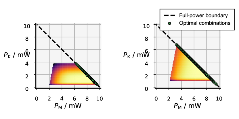
Figure 2: The optimal combinations of $P_{\mathrm{M}}$ and $P_{\mathrm{K}}$ in case of $P_{\mathrm{\Sigma}}=$10\text{\,}\mathrm{mW}$$, with $d_{\mathrm{K}}=30$ (left) and $d_{\mathrm{K}}=60$ (right).

V-B Deception Rate Surface

To gain insight into the deception rate surface $R_{\mathrm{d}}$ under the full-power transmission scheme, we set $P_{\mathrm{\Sigma}}=$10\text{\,}\mathrm{mW}$$, $z_{\mathrm{Eve}}=$-10\text{\,}\mathrm{dB}$$, $d_{\mathrm{M}}=16$, and computed $R_{\mathrm{d}}$ in the region $(P_{\mathrm{M}},d_{\mathrm{K}})\in[0,$10\text{\,}\mathrm{mW}$]\times\{0,1,...64\}$ with $\varepsilon^{\mathrm{th}}_{\mathrm{LF}}=0.5$. The result is illustrated in Fig. 3, where the feasible region defined by constraints (III-D)–(III-D) is highlighted with greater opacity compared to the rest.

From this figure, we observe that within the feasible region, the deception rate $R_{\mathrm{d}}$ exhibits concavity with respect to both $P_{\mathrm{M}}$ and $d_{\mathrm{K}}$. However, the behavior regarding convexity or concavity outside this region appears to be more complex.

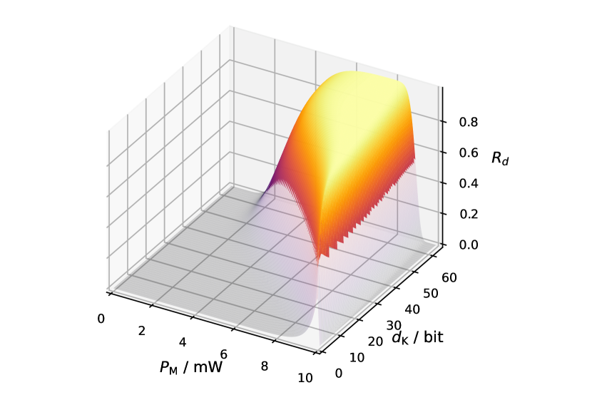
Figure 3: Deception rate under full-power transmission with $\varepsilon^{\mathrm{th}}_{\mathrm{LF}}=0.5.$

V-C Convergence Test of the Optimization Algorithm

To assess the practicality of the proposed BCD algorithm in optimizing both key length and power allocation, we conducted Monte-Carlo simulations with $P_{\mathrm{\Sigma}}=$10\text{\,}\mathrm{mW}$$, $z_{\mathrm{Eve}}=$-10\text{\,}\mathrm{dB}$$, and $\varepsilon^{\mathrm{th}}_{\mathrm{LF}}=0.5$. The algorithm was evaluated with two different lengths of the payload message: $d_{\mathrm{M}}=16$ and $d_{\mathrm{M}}=24$ respectively.

The results presented in Fig. 4 indicate that the BCD algorithm effectively reaches convergence in both cases, obtaining the optimum after 7 and 8 iterations, respectively. From this figure, it is observed that there is a tiny gap between the local optimum obtained by the BCD algorithm and the global optimum found by exhaustive search, which is attributed to the flatness of the region surrounding the optimal point. The error between the final step of the BCD algorithm and the global optimum is $2.836\times 10^{-6}$ for $d_{\mathrm{M}}=16$, and $1.166\times 10^{-4}$ for $d_{\mathrm{M}}=24$.

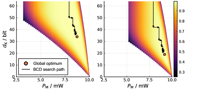
Figure 4: The $R_{\mathrm{d}}$ surface and the search path, with $d_{\mathrm{M}}=16$ (left) and $d_{\mathrm{M}}=24$ (right).

V-D Performance Evaluation

To evaluate the secrecy and deception performances of our proposed approach, we focus on the LFP $\varepsilon_{\mathrm{LF}}$ and the effective deception rate $R_{\mathrm{d}}$, respectively.

First, we set $P_{\Sigma}=$3\text{\,}\mathrm{mW}$$ and $\varepsilon^{\mathrm{th}}_{\mathrm{LF}}=0.5$, then evaluated our method under various eavesdropping channel conditions. For benchmarking purpose, we also measured the LFP of two conventional PLS approaches as baselines. Both the baseline solutions apply no deceptive ciphering ($d_{\mathrm{K}}=0$, $P_{\mathrm{K}}=0$), so they are incapable of deceiving but only minimizing $\varepsilon_{\mathrm{LF}}$. The first baseline selects the optimal $P_{\mathrm{M}}\in\left[0,P_{\mathrm{\Sigma}}\right]$ regarding a fixed $d_{\mathrm{M}}=16$, while the second searches for the best $d_{\mathrm{M}}\in[16,64]$ for a full-power transmission $P_{\mathrm{M}}=P_{\mathrm{\Sigma}}$.

The results are displayed in Fig. 5. Our PLD solution is able to maintain a satisfactory LFP that is significantly lower than the preset threshold $\varepsilon_{\mathrm{LF}}^{\mathrm{th}}$, while exhibiting a high effective deception rate. Especially, our method is not only robust to the eavesdropping channel gain, but even slightly benefiting from a reasonably good $z_{\mathrm{Eve}}$. In contrast, both baselines, performing closely to each other, logarithmically increase in LFP as $z_{\mathrm{Eve}}$ increases. This allows our PLD solution to outperform the baselines by a significant LFP margin over good eavesdropping channels, while simultaneously delivering an excellent deception rate up over $95\%$. On the other hand, when the eavesdropping channel gain is poor, our method is still well capable of deceiving Eve with $R_{\mathrm{d}}>75\%$, at only a reasonable cost of increased LFP regarding the baselines.

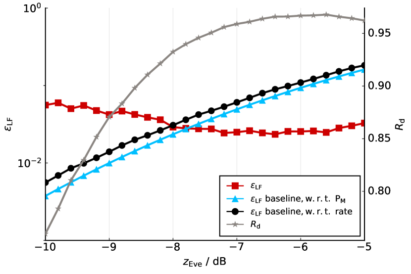
Figure 5: Results of sensitivity test regarding $z_{\mathrm{Eve}}$.

Next, we set $z_{\mathrm{Eve}}=-$5\text{\,}\mathrm{dB}$$, $\varepsilon^{\mathrm{th}}_{\mathrm{LF}}=0.5$ and evaluated our method under varying power budgets $P_{\mathrm{\Sigma}}$. The results are shown in Fig. 6. With an adequate power budget, the $\varepsilon_{\mathrm{LF}}$ decreases notably compared to the baseline, along with a high effective deception rate. Additionally, unlike traditional PLS solutions, which do not benefit or benefit little from increased power budgets, our method performs significantly better by increasing $P_{\mathrm{\Sigma}}$.

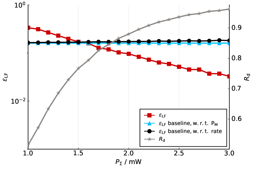
Figure 6: Results of sensitivity test regarding $P_{\Sigma}$.

The outcomes of a more comprehensive benchmark test, which combines various $z_{\mathrm{Eve}}$ and $P_{\mathrm{\Sigma}}$, are depicted in Fig. 7. We still kept the setup $\varepsilon^{\mathrm{th}}_{\mathrm{LF}}=0.5$. These results demonstrate that our method generally outperforms the classical PLS baselines with an adequate power budget under various eavesdropping channel conditions. In more detail, the minimum $P_{\mathrm{\Sigma}}$ required for our approach to surpass baseline performance increases as the channel gain difference $z_{\mathrm{Bob}}-z_{\mathrm{Eve}}$ becomes larger.

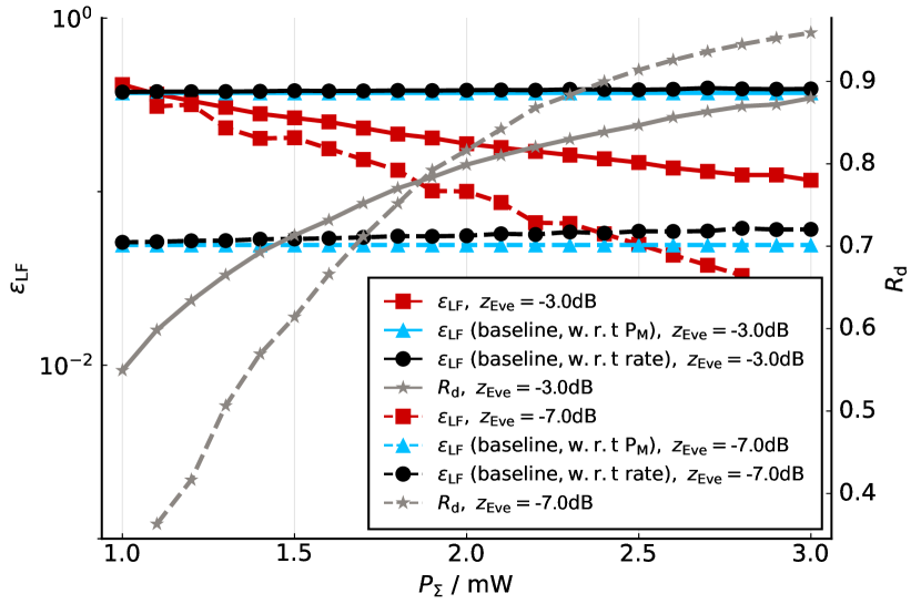
Figure 7: Benchmark results

In the previous experiments, we maintained the setup $\varepsilon^{\mathrm{th}}_{\mathrm{LF}}=0.5$. Given that the threshold of LFP $\varepsilon^{\mathrm{th}}_{\mathrm{LF}}$ influences the feasible region and potentially the optimum’s value, we designed an experiment to explore the impact of this constraint on the deception rate. Specifically, we focused on how the deception rate $R_{\mathrm{d}}$ changes with respect to $\varepsilon^{\mathrm{th}}_{\mathrm{LF}}$.

We set $P_{\Sigma}=$2\text{\,}\mathrm{mW}$$ and measured $\varepsilon_{\mathrm{LF}}$ as well as $R_{\mathrm{d}}$ regarding $\varepsilon^{\mathrm{th}}_{\mathrm{LF}}$ under various $z_{\mathrm{Eve}}$. Remarkably, neither $R_{\mathrm{d}}$ nor $\varepsilon_{\mathrm{LF}}$ is influenced by $\varepsilon_{\mathrm{LF}}^{\mathrm{th}}$. Their optima remain constants under certain channel conditions, as listed in Tab. III. Nevertheless, it is worth noting that the selection of $\varepsilon_{\mathrm{LF}}^{\mathrm{th}}$ significantly impacts the feasible region size of the problem. Given a certain transmission power budget, the feasible region shrinks with decreasing $\varepsilon^{\mathrm{th}}_{\mathrm{LF}}$. In fact, when $z_{\mathrm{Eve}}=-$3\text{\,}\mathrm{dB}$$ and $\varepsilon^{\mathrm{th}}_{\mathrm{LF}}=0.1$, no feasible region exists under the constraints (III-D–III-D). In such cases, one option is to accept a sub-optimal solution with reduced transmission power, where $P_{\mathrm{M}}+P_{\mathrm{K}}<P_{\mathrm{\Sigma}}$. Alternatively, one can adjust the blocklength $n$ of each packet.

TABLE III: Benchmark results regarding $\varepsilon_{\mathrm{LF}}^{\mathrm{th}}$ with $P_{\Sigma}=$2\text{\,}\mathrm{mW}$$

$z_{\mathrm{Eve}}$	$-3\text{\,}\mathrm{dB}$	$-5\text{\,}\mathrm{dB}$	$-7\text{\,}\mathrm{dB}$
$\varepsilon_{\mathrm{LF}}$	$0.1886^{*}$	0.0964	0.1003
$\varepsilon_{\mathrm{LF}}$ (baseline w.r.t $P_{\mathrm{M}}$)	0.3708	0.1611	0.0492
$\varepsilon_{\mathrm{LF}}$ (baseline w.r.t rate)	0.3840	0.1732	0.0557
$R_{\mathrm{d}}$	$0.7989^{*}$	0.8800	0.8163
*: The feasible region vanishes with full-power transmission, sub-optimum taken instead.

Additionally, we designed experiments to investigate how the minimum $\varepsilon^{\mathrm{th}}_{\mathrm{LF}}$, required to ensure the existence of a feasible solution, varies with the total power $P_{\mathrm{\Sigma}}$. The results are depicted in Fig. 8. From the figure, it is evident that as the total power $P_{\mathrm{\Sigma}}$ increases, the minimum $\varepsilon^{\mathrm{th}}_{\mathrm{LF}}$ required to maintain a feasible region becomes progressively smaller.

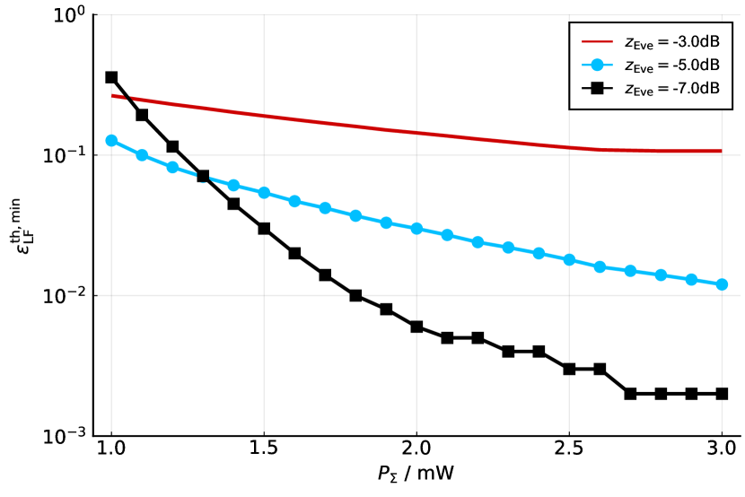
Figure 8: The minimal LFP threshold to have a feasible region.

VI Discussions

VI-A Use Cases

Upon the specific use scenario, our PLD approach can be applied on either the user plane (UP) or the control plane (CP). For UP application scenarios, merely a single counterfeit message shall suffice to significantly undermine the eavesdropper’s interests, relying solely on the effectiveness of deception. Typical use cases of this kind are including, but not limited to, military communications, police operations, and confidential business negotiations. When applied on the CP, in contrast, the focus is inducing the eavesdropper to expose itself, which relies on an appropriate radio interface protocol design that well merges the PLD strategy with its authentication procedure.

VI-B Ciphering Codec Design

For the deceptive ciphering algorithm $f:\mathbb{P}\times\mathbb{K}\to\mathbb{M}$, it is essential to satisfy Eq. (3) and Eq. (4). The former ensures that the eavesdropper cannot estimate the cipherer activation status from the decoded ciphertext $m$, and the latter invalidates the eavesdropping strategy of attempting to decrypt the ciphertext with a random key. However, these essential requirements propose a challenge to the ciphering codec design, especially when PLD is applied on the UP. On the one hand, it can become a conundrum to satisfy both of them when the cardinality of $\mathbb{M}$ is large. On the other hand, a small $\left|\mathbb{M}\right|$ will harshly limit the amount of information carried by each single message. Though this may not be a serious issue for the on CP where only limited amount of commands are available, it will be a significant challenge for generic UP application scenarios where a large amount of information needs to be transmitted. Forcing to use a $\mathbb{M}$ with small cardinality in such scenarios will break semantically complete information into multiple codewords, which not only reduces the impairment of the eavesdropper’s interests that can be caused by one single false message, but also allows the eavesdropper to leverage its semantic knowledge for coherence analysis on the multiple messages, and therewith avoid being deceived.

A potential solution to this challenge is to combine PLD with semantic communications. By deploying paired semantic encoder and decoder on both sides of the communication link, it is not only significantly reducing the raw data rate required to deliver the same amount of semantic information, but also effectively constraining the feasible region of codewords.

VI-C Peak-to-Average Power Ratio

Regarding Theorem 1 that our approach always prefers full-power transmission, it is not only beneficial for the simplification of the optimization, but also for the reduction of the Peak-to-Average Power Ratio (PAPR) of the transmitted signal. Regardless the measured legitimate channel gain $z_{\mathrm{Bob}}$ or the estimated eavesdropping channel gain $z_{\mathrm{Eve}}$, the transmitter always maintains a consistent transmission power across all messages. Combined with symbol-level PAPR reducing techniques, such as Discrete Fourier Transform-spread-OFDM (DFT-s-OFDM), it can provide an outstanding performance in terms of power efficiency and linearity of the power amplifier, which is crucial in practical implementation of wireless transceivers.

VI-D Orthogonal Frequency-Division Multiplexing

While NOM is promising in terms of performance, it lacks compatibility with conventional wireless standards. Adopting our PLD approach in orthogonal frequency-division multiplexing (OFDM) systems appear therefore an attractive alternative. In an OFDM frame, the radio resource, managed in terms of physical resource blocks (PRBs), can be allocated between the ciphertext and the key in the time-frequency domain. This design frees the receiver from the SIC operation, as the key and the ciphertext are independently decoded in parallel, which reduces the hardware complexity. However, unlike the transmission power that can be arbitrarily divided, the PRBs can only be allocated in integer numbers, which may lead to a less optimality in comparison to the NOM solution.

VI-E Multi-Access

Though this work mainly focuses on the point-to-point communication scenario, the PLD approach can also be extended to wireless network scenarios, where the multi-access scheme must be well considered.

The multi-access solution is strongly related to the selection of ciphertext-key multiplexing scheme. As cascaded SIC is likely leading to a high error rate in key decoding, we do not recommend applying NOMA on top of NOM-based PLD, but orthogonal multiple access (OMA) solutions such like orthogonal frequency-division multiple access (OFDMA) or simple time-division multiple access (TDMA). However, if the ciphertext and key are orthogonally multiplexed like discussed in Sec. VI-D, NOMA can be considered as a feasible solution to achieve a higher spectral efficiency.

VII Conclusion

In this work, we have proposed a comprehensive design for a novel PLD approach that integrates Physical Layer Security PLS with deception technology. Jointly optimizing the transmission power and encryption key length, we are able to maximize the effective deception rate under a given constraint of LFP, simultaneously achieving both secrecy and reliability of communication. We have proved that the optimal power allocation always fully utilizes the transmission power budget, and proposed an efficient algorithm to solve the corresponding optimization problem. The numerical results have demonstrated the superiority of our approach over conventional PLS solutions in terms of both secrecy and deception performance. Further, we have discussed the potential use cases, the challenges in ciphering codec design, the benefits of the full-power transmission scheme, and the potential extensions of our approach to OFDM systems and multi-access scenarios.

Appendix A Proof of Theorem 1

Proof.

This theorem can be proven by the contradiction. First, with a given $d_{\mathrm{K}}$, we define the following auxiliary function to ease the notation:

$$\varepsilon_{i,j}(P)\triangleq\varepsilon_{i,j}|_{P_{j}=P},\forall(i,j)\in\{\text{Bob},\text{Eve}\}\times\{\text{M},\text{K}\},$$ (17)

Suppose there exists an optimal power allocation $\left(P^{\mathrm{o}}_{\mathrm{K}},P^{\mathrm{o}}_{\mathrm{M}}\right)$ that leaves from the power budget a positive residual $P_{\Delta}=P_{\Sigma}-P^{\mathrm{o}}_{\mathrm{K}}-P^{\mathrm{o}}_{\mathrm{M}}>0$. Since it is optimal, for any feasible power allocation $\left(P_{\mathrm{M}},P_{\mathrm{K}}\right)$ it must hold that

$$R_{\text{d}}\left(P^{\mathrm{o}}_{\mathrm{M}},P^{\mathrm{o}}_{\mathrm{K}}\right)\geqslant R_{\text{d}}\left(P_{\mathrm{M}},P_{\mathrm{K}}\right).$$ (18)

Meanwhile, there is always another feasible allocation $(P^{\mathrm{f}}_{\mathrm{M}},P^{\mathrm{o}}_{\mathrm{K}})$ where $P^{\mathrm{f}}_{\mathrm{M}}=P^{\mathrm{o}}_{\mathrm{M}}+P_{\Delta}$. Given the same $P_{\mathrm{K}}$, it can be straightforwardly shown that $\varepsilon_{\text{Bob,M}}$ and $\varepsilon_{\text{Eve,M}}$ are monotonically decreasing in $P_{\mathrm{M}}$ with:

$$\begin{split}\frac{\partial R_{\text{d}}}{\partial P_{\mathrm{M}}}&=-\frac{\partial\varepsilon_{\text{Bob,M}}}{\partial P_{\mathrm{M}}}(1-\varepsilon_{\text{Eve,M}})\varepsilon_{\text{Eve,K}}\\ &~{}~{}~{}~{}~{}~{}~{}~{}-\frac{\partial\varepsilon_{\text{Eve,M}}}{\partial P_{\mathrm{M}}}(1-(1-\varepsilon_{\text{Bob,M}}))\varepsilon_{\text{Bob,K}}\\ &\geqslant 0.\end{split}$$ (19)

The inequality holds since we have the following derivative based on the chain rule:

$$\begin{split}\frac{\partial\varepsilon_{i,\text{M}}}{\partial P_{\mathrm{M}}}&=\frac{\partial\varepsilon_{i,\text{M}}}{\partial\omega_{i,\text{M}}}\frac{\partial\omega_{i,\text{M}}}{\partial\gamma_{i,\text{M}}}\frac{\partial\gamma_{i,\text{M}}}{\partial P_{\mathrm{M}}}\leqslant 0,\end{split}$$ (20)

where $\omega_{i,j}=\sqrt{\frac{n}{V(\gamma_{i,j})}}(\mathcal{C}(\gamma_{i,j})-\frac{d_{j}}{n})$ is a auxiliary function. Therefore, it always holds that

$$\varepsilon_{\text{Bob,M}}(P^{\mathrm{o}}_{\mathrm{M}}) >\varepsilon_{\text{Bob,M}}\left(P^{\mathrm{f}}_{\mathrm{M}}\right),$$ (21)

$$\varepsilon_{\text{Eve,M}}(P^{\mathrm{o}}_{\mathrm{M}}) >\varepsilon_{\text{Eve,M}}\left(P^{\mathrm{f}}_{\mathrm{M}}\right)$$ (22)

Then, we have:

$$\begin{split}&R_{\text{d}}\left(P^{\mathrm{f}}_{\mathrm{M}},P^{\mathrm{o}}_{\mathrm{K}}\right)-R_{\text{d}}\left(P^{\mathrm{o}}_{\mathrm{M}},P^{\mathrm{o}}_{\mathrm{K}}\right)\\ =&\left[1-2\varepsilon_{\text{Bob,K}}\left(P^{\mathrm{o}}_{\mathrm{K}}\right)\right]\left[\varepsilon_{\text{Bob,M}}\left(P^{\mathrm{o}}_{\mathrm{M}}\right)-\varepsilon_{\text{Bob,M}}\left(P^{\mathrm{f}}_{\mathrm{M}}\right)\right]\\ &-\left[1-2\varepsilon_{\text{Eve,K}}\left(P^{\mathrm{o}}_{\mathrm{K}}\right)\right]\left[\varepsilon_{\text{Eve,M}}\left(P^{\mathrm{o}}_{\mathrm{M}}\right)-\varepsilon_{\text{Eve,M}}\left(P^{\mathrm{f}}_{\mathrm{M}}\right)\right]\\ >&0.\end{split}$$ (23)

The inequality above holds, since $2\varepsilon_{\text{Bob,K}}\leqslant 2\varepsilon^{\mathrm{th}}_{\text{Bob,K}}<1$ and $2\varepsilon_{\text{Eve,K}}\geqslant 2\varepsilon^{\mathrm{th}}_{\text{Eve,K}}>1$. In other words, the solution $P^{\mathrm{f}}_{\mathrm{K}}$ and $P^{\mathrm{f}}_{\mathrm{M}}$ achieves a better deception rate $R_{\text{d}}\left(P^{\mathrm{f}}_{\mathrm{M}},P^{\mathrm{o}}_{\mathrm{K}}\right)$ than $R_{\text{d}}\left(P^{\mathrm{o}}_{\mathrm{M}},P^{\mathrm{o}}_{\mathrm{K}}\right)$, which violates the assumption of optimum. ∎

Appendix B Proof of Lemma 1

Proof.

First, we introduce a constant $\lambda(\hat{d}_{\mathrm{K}}^{(q)},\hat{P}_{\mathrm{M}}^{(q)})=\frac{(1-\varepsilon_{\text{Bob},D}(\hat{d}_{\mathrm{K}}^{(q)},\hat{P}_{\mathrm{M}}^{(q)}))}{\varepsilon_{\text{Eve},D}((\hat{d}_{\mathrm{K}}^{(q)},\hat{P}_{\mathrm{M}}^{(q)}))}$ at the local point $(\hat{d}_{\mathrm{K}}^{(q)},\hat{P}_{\mathrm{M}}^{(q)})$. Since $0\leqslant\varepsilon_{i,D}\leqslant 1$, it is trivial to show that $\lambda$ is always non-negative. Then, we have:

$$R_{\text{d}}=\frac{\lambda}{\lambda}(1-\varepsilon_{\text{Bob},D})\varepsilon_{\text{Eve},D}=\frac{1}{\lambda}(1-\varepsilon_{\text{Bob},D})\cdot\lambda\varepsilon_{\text{Eve},D}$$ (24)

Then, based on the inequality of arithmetic and geometric means, we can reconstruct the upper-bound of $R_{\text{d}}$ as:

$$\begin{split}&\sqrt{\lambda R_{\text{d}}}\leqslant\frac{(1-\varepsilon_{\text{Bob},D})+\lambda\varepsilon_{\text{Eve},D}}{2}\\ \Longleftrightarrow&\lambda R_{\text{d}}\leqslant\left(\frac{(1-\varepsilon_{\text{Bob},D})+\lambda\varepsilon_{\text{Eve},D}}{2}\right)^{2}\\ \Longleftrightarrow&R_{\text{d}}\leqslant\frac{1}{4\lambda}\left((1-\varepsilon_{\text{Bob},D})+\lambda\varepsilon_{\text{Eve},D}\right)^{2}\triangleq\hat{R}_{\mathrm{d}},\end{split}$$ (25)

which completes the proof. ∎

Appendix C Proof of Lemma 2

Proof.

• We start with the objective function $\hat{R}_{d}$. To prove its convexity, we first investigate the monotonicity of $\varepsilon_{i,j}$ with respect to $d_{\mathrm{K}}$. In particular, we have

  $$\frac{\partial\varepsilon_{i,\text{M}}}{\partial d_{\mathrm{K}}}=0,$$ (26)

  and

  $$\begin{split}\frac{\partial\varepsilon_{i,\text{K}}}{\partial d_{\mathrm{K}}}&=\frac{\partial\varepsilon_{i,\text{K}}}{\partial\omega_{i,\text{K}}}\frac{\partial\omega_{i,\text{K}}}{\partial d_{\mathrm{K}}}\\ &=e^{-\frac{\omega^{2}_{i,K}}{2}}\sqrt{\frac{n}{V_{i,K}}}\cdot\frac{1}{n}\geqslant 0.\end{split}$$ (27)

  Therefore, $\varepsilon_{\text{Bob},K}$ and $\varepsilon_{\text{Eve},K}$ are monotonically increasing in $d_{\mathrm{K}}$. Then, we further investigate the convexity of $\varepsilon_{i,j}$. Their second derivatives are:

  $$\frac{\partial^{2}\varepsilon_{i,\text{M}}}{\partial^{2}d_{\mathrm{K}}}=0,$$ (28)

  and

  $$\begin{split}\frac{\partial^{2}\varepsilon_{i,\text{K}}}{\partial^{2}d_{\mathrm{K}}}&=\frac{\partial^{2}\varepsilon_{i,\text{K}}}{\partial\omega_{i,\text{K}}^{2}}\underbrace{\left(\frac{\partial\omega_{i,\text{K}}}{\partial d_{\mathrm{K}}}\right)^{2}}_{\geqslant 0}+\underbrace{\frac{\partial\varepsilon_{i,\text{K}}}{\partial\omega_{i,\text{K}}}\frac{\partial^{2}\omega_{i,\text{K}}}{\partial d_{\mathrm{K}}^{2}}}_{=0}.\end{split}$$ (29)

  Note that $\varepsilon_{i,j}(\omega_{i,j})$ is a Q-function, which is convex if $\omega_{i,j}$ is non-negative and concave if it is non-positive. It indicates that $\varepsilon_{i,\text{K}}$ is convex in $d_{\mathrm{K}}$ if $\omega_{i,\text{K}}\geqslant 0$ while being concave if $\omega_{i,\text{K}}\leqslant 0$. Recall that the transmission must fulfill $\varepsilon_{\text{Bob},K}\leqslant\varepsilon_{\text{Bob},K}^{\text{th}}\leqslant 0.5$ and $\varepsilon_{\text{Eve},K}\geqslant\varepsilon_{\text{Eve},K}^{\text{th}}\geqslant 0.5$. Therefore, for any feasible $d_{\mathrm{K}}$, it must hold that

  $$\omega_{\text{Bob},K}=\sqrt{\frac{n}{V(\gamma_{\text{Bob},K}}}(\mathcal{C}(\gamma_{\text{Bob},K}-\frac{d_{\mathrm{K}}}{n})\geqslant Q^{-1}(\varepsilon_{\text{Bob},K}^{\text{th}})\geqslant 0,$$ (30)

  and

  $$\omega_{\text{Eve},K}=\sqrt{\frac{n}{V(\gamma_{\text{Eve},K}}}(\mathcal{C}(\gamma_{\text{Eve},K}-\frac{d_{\mathrm{K}}}{n})\leqslant Q^{-1}(\varepsilon_{\text{Eve},K}^{\text{th}})\leqslant 0,$$ (31)

  where $Q^{-1}(\cdot)$ is the inverse Q-function. Therefore, $\varepsilon_{\text{Bob},K}$ is a convex and decreasing function while $\varepsilon_{\text{Eve},K}$ being a concave and decreasing function. Recall that $\hat{R}_{d}$ is the quadratic function of $\frac{1}{R_{b}}$, $\frac{1}{1-\varepsilon_{\text{Eve},K}}$ and $\frac{1}{\varepsilon_{\text{Eve},M}}$ according to (13). Then, $\hat{R}_{d}$ is convex, if each of the components, i.e., $R_{b}$, $(1-\varepsilon_{\text{Eve},M})$ and $\varepsilon_{\text{Eve},K}$, is concave and non-negative. Clearly, both this is true for $(1-\varepsilon_{\text{Eve},M})$ and $\varepsilon_{\text{Eve},K}$. Therefore, we focus on the concavity of $R_{b}$ with its second derivative, i.e.,

  $$\begin{split}\frac{\partial^{2}R_{b}}{\partial d_{\mathrm{K}}^{2}}=-(1-\varepsilon_{\text{Bob,M}})\underbrace{\frac{\partial^{2}\varepsilon_{\text{Bob,K}}}{\partial d_{\mathrm{K}}^{2}}}_{\geqslant 0}-\underbrace{\frac{\partial\varepsilon_{\text{Bob,K}}}{\partial d_{\mathrm{K}}}}_{\geqslant 0}\leqslant 0.\end{split}$$ (32)

  Hence, $R_{b}$ is indeed concave, i.e., $\hat{R}_{\mathrm{d}}$ is convex. It is also trivial to show that all the constraints are either convex or linear, i.e., the feasible set of Problem (1) is convex. Then, since the objective function to be maximized is concave and its feasible set is convex, Problem (1) is a convex problem.

∎

$$\begin{split}&\frac{\partial^{2}\varepsilon_{i,\text{M}}}{\partial P_{\mathrm{M}}^{2}}=\frac{\partial\varepsilon_{i,\text{M}}}{\partial\gamma_{i,\text{M}}}\frac{\partial^{2}\gamma_{i,\text{M}}}{\partial P_{\mathrm{M}}^{2}}+\frac{\partial^{2}\varepsilon_{i,\text{M}}}{\partial\gamma^{2}_{i,\text{M}}}\left(\frac{\partial\gamma_{i,\text{M}}}{\partial P_{\mathrm{M}}}\right)^{2}\\ =&\frac{1}{\sqrt{2\pi}}e^{-\frac{\omega_{i,\text{M}}}{2}}\left(\frac{\partial\omega_{i,\text{M}}}{\partial\gamma_{i,\text{M}}}\left(\omega_{i,\text{M}}\frac{\partial\omega_{i,\text{M}}}{\partial\gamma_{i,\text{M}}}\left(\frac{\partial\gamma_{i,\text{M}}}{\partial P_{\mathrm{M}}}\right)^{2}-\frac{\partial^{2}\gamma_{i,\text{M}}}{\partial P_{\mathrm{M}}^{2}}\right)-\underbrace{\frac{\partial^{2}\omega_{i,\text{M}}}{\partial\gamma^{2}_{i,\text{M}}}\left(\frac{\partial\gamma_{i,\text{M}}}{\partial P_{\mathrm{M}}}\right)^{2}}_{\leqslant 0}\right)\\ \geqslant&\frac{1}{\sqrt{2\pi}}e^{-\frac{\omega_{i,\text{M}}}{2}}\frac{\partial\omega_{i,\text{M}}}{\partial\gamma_{i,\text{M}}}\left(\omega_{i,\text{M}}\frac{\partial\omega_{i,\text{M}}}{\partial\gamma_{i,\text{M}}}\left(\frac{\partial\gamma_{i,\text{M}}}{\partial P_{\mathrm{M}}}\right)^{2}-\frac{\partial^{2}\gamma_{i,\text{M}}}{\partial P_{\mathrm{M}}^{2}}\right)\\ =&\frac{1}{\sqrt{2\pi}}e^{-\frac{\omega_{i,\text{M}}}{2}}\frac{\partial\omega_{i,\text{M}}}{\partial\gamma_{i,\text{M}}}\left(\omega_{i,\text{M}}\frac{\partial\omega_{i,\text{M}}}{\partial\gamma_{i,\text{M}}}\frac{z^{2}_{1}(z_{i}P_{\Sigma}+\sigma^{2}_{i})^{2}}{(z_{i}P_{\mathrm{K}}+\sigma^{2}_{i})^{4}}-\frac{2z_{i}^{2}(z_{i}P_{\Sigma}+\sigma^{2}_{i})}{(z_{i}P_{\mathrm{K}}+\sigma^{2}_{i})^{3}}\right)\\ =&\frac{1}{\sqrt{2\pi}}e^{-\frac{\omega_{i,\text{M}}}{2}}\frac{\partial\omega_{i,\text{M}}}{\partial\gamma_{i,\text{M}}}\frac{z_{i}^{2}(z_{i}P_{\Sigma}+\sigma^{2}_{i})}{(z_{i}P_{\mathrm{K}}+\sigma^{2}_{i})^{3}}\left(\omega_{i,\text{M}}\frac{\partial\omega_{i,\text{M}}}{\partial\gamma_{i,\text{M}}}\underbrace{\frac{(z_{i}P_{\Sigma}+\sigma^{2}_{i})}{(z_{i}P_{\mathrm{K}}+\sigma^{2}_{i})}}_{\geqslant\gamma_{i,\text{M}}}-2\right)\\ \geqslant&\frac{1}{\sqrt{2\pi}}e^{-\frac{\omega_{i,\text{M}}}{2}}\frac{\partial\omega_{i,\text{M}}}{\partial\gamma_{i,\text{M}}}\frac{z_{i}^{2}(z_{i}P_{\Sigma}+\sigma^{2}_{i})}{(z_{i}P_{\mathrm{K}}+\sigma^{2}_{i})^{3}}\left(\omega_{i,\text{M}}\frac{\partial\omega_{i,\text{M}}}{\partial\gamma_{i,\text{M}}}\gamma_{i,\text{M}}-2\right)\geqslant\frac{6.25\gamma_{i,\text{M}}}{\sqrt{\gamma_{i,\text{M}}(\gamma_{i,\text{M}}+1)}}-2\geqslant 0,\end{split}$$ (34)

 

Appendix D Proof of Theorem 2

Proof.

Similar to the proof of Lemma 2, we start with the convexity of the objective function $\hat{R}_{d}$. We also first investigate the monotonicity of $\varepsilon_{i,M}$ with respect $P_{M}$ as follows:

$$\begin{split}\frac{\partial\varepsilon_{i,\text{M}}}{\partial P_{\mathrm{M}}}&=\frac{\partial\varepsilon_{i,\text{M}}}{\partial\gamma_{i,\text{M}}}\frac{\partial\gamma_{i,\text{M}}}{\partial P_{\mathrm{M}}}=\underbrace{\frac{\partial\varepsilon_{i,\text{M}}}{\partial\gamma_{i,\text{M}}}}_{\leqslant 0}\frac{2z_{i}^{2}(z_{i}P_{\Sigma}+\sigma^{2})}{(z_{i}P_{\mathrm{K}}+\sigma^{2})^{3}}\leqslant 0.\end{split}$$ (33)

Note that the above inequality holds with the constraints (III-D) and (III-D), i.e., $\omega_{i,M}\geqslant 0$. Moreover, since $n\geqslant 10$ and $\varepsilon_{i,\text{M}}\leqslant\varepsilon^{\mathrm{th}}_{i,\text{M}}<0.5$, we can proven that $\varepsilon_{i,M}$ is convex in $P_{M}$ with  (33) and  (34). Note that the inequality in (34) holds with $\gamma_{i,M}\geqslant\gamma_{th}\geqslant 1$, which is required to fulfill the error probability constraints in practical scenarios [41].

Similarly, we can show that $\varepsilon_{\text{Bob},K}$ is convex while $\varepsilon_{\text{Eve},K}$ being concave with

$$\frac{\partial\gamma_{i,\text{K}}}{\partial P_{\mathrm{M}}}=-\frac{z_{i}}{\sigma^{2}},~{}\frac{\partial^{2}\gamma_{i,\text{K}}}{\partial P_{\mathrm{M}}^{2}}=0.\vspace{-5pt}$$ (35)

To avoid repetition, we omit the details. Note that the convexity/concavity of $\varepsilon_{\text{Bob},K}$ differs from the ones of $\varepsilon_{\text{Eve},K}$. This is due to the fact that $\omega_{\text{Bob},K}\geqslant 0$ and $\omega_{\text{Eve},K}\leqslant 0$ according to the constraints (III-D) and (III-D).

With the above results, it is clear that $\frac{1}{\varepsilon_{\text{Eve},K}}$ and $\frac{1}{1-\varepsilon_{\text{Eve},M}}$ are both convex in $P_{M}$, since a convex and decreasing function composed with a concave function is also convex [42]. However, we still need to determine the convexity of $R_{b}$. In particular, its second-order derivative is:

$$\begin{split}\frac{\partial^{2}R_{b}}{\partial P_{\mathrm{M}}^{2}}=&-\frac{\partial^{2}\varepsilon_{\text{Bob},K}}{\partial P_{\mathrm{M}}^{2}}+\frac{\partial^{2}\varepsilon_{\text{Bob},M}}{\partial P_{\mathrm{M}}^{2}}\varepsilon_{\text{Bob},K}+\frac{\partial^{2}\varepsilon_{\text{Bob},K}}{\partial P_{\mathrm{M}}^{2}}\varepsilon_{\text{Bob},M}\\ &+\frac{\partial\varepsilon_{\text{Bob},K}}{\partial P_{\mathrm{M}}}\frac{\varepsilon_{\text{Bob},M}}{\partial P_{\mathrm{M}}}\\ =&-(1-\varepsilon_{\text{Bob},M})\underbrace{\frac{\partial^{2}\varepsilon_{\text{Bob},K}}{\partial P_{\mathrm{M}}^{2}}}_{\geqslant 0}+\underbrace{\frac{\partial^{2}\varepsilon_{\text{Bob},M}}{\partial P_{\mathrm{M}}^{2}}}_{\geqslant 0}\varepsilon_{\text{Bob},K}\\ &+\underbrace{\frac{\partial\varepsilon_{\text{Bob},K}}{\partial P_{\mathrm{M}}}}_{\geqslant 0}\underbrace{\frac{\varepsilon_{\text{Bob},M}}{\partial P_{\mathrm{M}}}}_{\leqslant 0}\leqslant\frac{\partial^{2}\varepsilon_{\text{Bob},M}}{\partial P_{\mathrm{M}}^{2}}-\frac{\partial^{2}\varepsilon_{\text{Bob},K}}{\partial P_{\mathrm{M}}^{2}}.\end{split}$$ (36)

Since the feasible $P_{M}$ must fulfill that $\varepsilon_{\text{Bob},j}\leqslant\varepsilon^{\text{th}}_{\text{Bob},j}\leqslant 0.1$ and $P_{K}=P_{\sum}-P_{M}$, we have $\varepsilon_{\text{Bob},K}\leqslant 10(1-\varepsilon_{\text{Bob},M})$, $P_{M}\geqslant P_{K}$ and $\gamma_{\text{Bob},M}\leqslant\gamma_{\text{Bob},K}$. Therefore, it also indicates that $\omega(\gamma_{\text{Bob},M},d_{M})\leqslant\omega(\gamma_{\text{Bob},M},d_{\mathrm{K}})\leqslant\omega(\gamma_{\text{Bob},K},d_{\mathrm{K}})$. Note that both $\varepsilon_{\text{Bob},M}$ and $\varepsilon_{\text{Bob},K}$ are error probability, which is characterized by the Q-function according to (12). Then, let denote $P_{0.5}$ the transmit power that achieves $\varepsilon_{\text{Bob},K}(P_{0.5})=0.5$ while $P_{\infty}$ the transmit power that achieves $\varepsilon_{\text{Bob},K}(P_{\infty})=0$. It holds that

$$\frac{\partial^{2}\varepsilon_{\text{Bob},M}}{\partial P_{0.5}^{2}}\leqslant\frac{\partial^{2}\varepsilon_{\text{Bob},K}}{\partial P_{0.5}^{2}}=0,~{}\frac{\partial^{2}\varepsilon_{\text{Bob},M}}{\partial P_{\infty}^{2}}=\frac{\partial^{2}\varepsilon_{\text{Bob},K}}{\partial P_{\infty}^{2}}>0,$$ (37)

Therefore, within the feasible set of Problem (2), we have $\frac{\partial^{2}R_{b}}{\partial P_{\mathrm{M}}^{2}}\leqslant\frac{\partial^{2}\varepsilon_{\text{Bob},M}}{\partial P_{\mathrm{M}}^{2}}-\frac{\partial^{2}\varepsilon_{\text{Bob},K}}{\partial P_{\mathrm{M}}^{2}}\leqslant 0$.

Since all components of $\hat{R}_{d}$ are convex, the objective function $\hat{R}_{d}$ is also convex. Moreover, it is trivial to show that all constraints are either convex or affine. As a result, Problem (2) is convex.

∎

References

- [1] J. M. Hamamreh, H. M. Furqan, and H. Arslan, “Classifications and applications of physical layer security techniques for confidentiality: A comprehensive survey,” IEEE Commun. Surv. Tutor., vol. 21, no. 2, pp. 1773–1828, 2019.
- [2] C. She et al., “A tutorial on ultra-reliable and low-latency communications in 6G: Integrating domain knowledge into deep learning,” Proc. IEEE, vol. 109, no. 3, pp. 204–246, 2021.
- [3] Y. Polyanskiy, H. V. Poor, and S. Verdu, “Channel coding rate in the finite blocklength regime,” IEEE Trans. Inf. Theory, vol. 56, no. 5, pp. 2307–2359, 2010.
- [4] W. Yang, R. F. Schaefer, and H. V. Poor, “Wiretap channels: Nonasymptotic fundamental limits,” IEEE Trans. Inf. Theory, vol. 65, no. 7, pp. 4069–4093, 2019.
- [5] L. Lv, D. Xu, R. Q. Hu et al., “Safeguarding next generation multiple access using physical layer security techniques: A tutorial,” arXiv preprint arXiv:2403.16477, 2024.
- [6] H. Xu, T. Yang, K.-K. Wong et al., “Achievable regions and precoder designs for the multiple access wiretap channels with confidential and open messages,” IEEE J. Sel. Areas Commun., vol. 40, no. 5, pp. 1407–1427, 2022.
- [7] C. Wang and Z. Lu, “Cyber deception: Overview and the road ahead,” IEEE Secur. Priv., vol. 16, no. 2, pp. 80–85, 2018.
- [8] B. Han, Y. Zhu, A. Schmeink et al., “Non-orthogonal multiplexing in the FBL regime enhances physical layer security with deception,” in 2023 IEEE 24th Int. Workshop Signal Process. Adv. Wirel. Commun. (SPAWC), 2023, pp. 211–215.
- [9] A. D. Wyner, “The wire-tap channel,” Bell Syst. Tech. J., vol. 54, no. 8, pp. 1355–1387, 1975.
- [10] C. E. Shannon, “Communication theory of secrecy systems,” Bell Syst. Tech. J., vol. 28, no. 4, pp. 656–715, 1949.
- [11] A. Carleial and M. Hellman, “A note on Wyner’s wiretap channel (corresp.),” IEEE Trans. Inf. Theory, vol. 23, no. 3, pp. 387–390, 1977.
- [12] S. Leung-Yan-Cheong and M. Hellman, “The Gaussian wire-tap channel,” IEEE Trans. Inf. Theory, vol. 24, no. 4, pp. 451–456, 1978.
- [13] P. K. Gopala, L. Lai, and H. El Gamal, “On the secrecy capacity of fading channels,” IEEE Trans. Inf. Theory, vol. 54, no. 10, pp. 4687–4698, 2008.
- [14] X. Zhou, R. K. Ganti, and J. G. Andrews, “Secure wireless network connectivity with multi-antenna transmission,” IEEE Trans. Wirel. Commun., vol. 10, no. 2, pp. 425–430, 2011.
- [15] I. Csiszar and J. Korner, “Broadcast channels with confidential messages,” IEEE Trans. Inf. Theory, vol. 24, no. 3, pp. 339–348, 1978.
- [16] E. Tekin and A. Yener, “The Gaussian multiple access wire-tap channel,” IEEE Trans. Inf. Theory, vol. 54, no. 12, pp. 5747–5755, 2008.
- [17] Y. Liang, A. Somekh-Baruch, H. V. Poor et al., “Capacity of cognitive interference channels with and without secrecy,” IEEE Trans. Inf. Theory, vol. 55, no. 2, pp. 604–619, 2009.
- [18] Y. Oohama, “Capacity theorems for relay channels with confidential messages,” in 2007 IEEE Int. Symp. Inf. Theory, 2007, pp. 926–930.
- [19] A. Mukherjee, S. A. A. Fakoorian, J. Huang et al., “Principles of physical layer security in multiuser wireless networks: A survey,” IEEE Commun. Surv. Tutor., vol. 16, no. 3, pp. 1550–1573, 2014.
- [20] D. Wang, B. Bai, W. Zhao et al., “A survey of optimization approaches for wireless physical layer security,” IEEE Commun. Surv. Tutor., vol. 21, no. 2, pp. 1878–1911, 2019.
- [21] B. Liu, P. Zhu, J. Li et al., “Energy-efficient optimization in distributed massive mimo systems for slicing embb and urllc services,” IEEE Trans. Veh. Technol., vol. 72, no. 8, pp. 10 473–10 487, 2023.
- [22] K. Li, P. Zhu, Y. Wang et al., “Joint uplink and downlink resource allocation toward energy-efficient transmission for urllc,” IEEE J. Sel. Areas Commun., vol. 41, no. 7, pp. 2176–2192, 2023.
- [23] C. Liu, S. Li, W. Yuan et al., “Predictive precoder design for otfs-enabled urllc: A deep learning approach,” IEEE J. Sel. Areas Commun., vol. 41, no. 7, pp. 2245–2260, 2023.
- [24] W. Yang, R. F. Schaefer, and H. V. Poor, “Wiretap channels: Nonasymptotic fundamental limits,” IEEE Trans. Inf. Theory, vol. 65, no. 7, pp. 4069–4093, 2019.
- [25] C. Wang, Z. Li, H. Zhang et al., “Achieving covertness and security in broadcast channels with finite blocklength,” IEEE Trans. Wirel. Commun., vol. 21, no. 9, pp. 7624–7640, 2022.
- [26] M. Oh, J. Park, and J. Choi, “Joint optimization for secure and reliable communications in finite blocklength regime,” IEEE Trans. Wirel. Commun., vol. 22, no. 12, pp. 9457–9472, 2023.
- [27] Y. Zhu, X. Yuan, Y. Hu et al., “Trade reliability for security: Leakage-failure probability minimization for machine-type communications in URLLC,” IEEE J. Sel. Areas Commun., vol. 41, no. 7, pp. 2123–2137, 2023.
- [28] K. Cao, B. Wang, H. Ding et al., “Improving physical layer security of uplink NOMA via energy harvesting jammers,” IEEE Trans. Inf. Forensics Security, vol. 16, pp. 786–799, 2021.
- [29] Z. Xiang, W. Yang, G. Pan et al., “Physical layer security in cognitive radio inspired NOMA network,” IEEE J. Sel. Topics Signal Process., vol. 13, no. 3, pp. 700–714, 2019.
- [30] K. D. Mitnick and W. L. Simon, The Art of Deception: Controlling the Human Element of Security. John Wiley & Sons, 2003.
- [31] B. Cheswick, “An evening with Berferd in which a cracker is lured, endured, and studied,” in Proc. Winter USENIX Conference, San Francisco, 1992, pp. 20–24.
- [32] C. Stoll, The Cuckoo’s Egg: Tracking a Spy Through the Maze of Computer Espionage. Simon and Schuster, 2005.
- [33] D. Fraunholz, S. D. Anton, C. Lipps et al., “Demystifying deception technology: A survey,” arXiv preprint arXiv:1804.06196, 2018.
- [34] X. Han, N. Kheir, and D. Balzarotti, “Deception techniques in computer security: A research perspective,” ACM Comput. Surv., vol. 51, no. 4, pp. 1–36, 2018.
- [35] J. Pawlick, E. Colbert, and Q. Zhu, “A game-theoretic taxonomy and survey of defensive deception for cybersecurity and privacy,” ACM Comput. Surv., vol. 52, no. 4, pp. 1–28, 2019.
- [36] Q. He, S. Fang, T. Wang et al., “Proactive anti-eavesdropping with trap deployment in wireless networks,” IEEE Trans. Dependable Secure Comput., vol. 20, no. 1, pp. 637–649, 2023.
- [37] P. Qi, Y. Meng, S. Zheng et al., “Adversarial defense embedded waveform design for reliable communication in the physical layer,” IEEE Internet Things J., vol. 11, no. 10, pp. 18 136–18 153, 2024.
- [38] W. Yang, R. F. Schaefer, and H. V. Poor, “Wiretap channels: Nonasymptotic fundamental limits,” IEEE Trans. Inf. Theory, vol. 65, no. 7, pp. 4069–4093, 2019.
- [39] D. R. Hunter and K. Lange, “Quantile regression via an MM algorithm,” J. Comput. Graph. Stat., vol. 9, no. 1, p. 60–77, Mar. 2000.
- [40] P. Tseng, “Convergence of a block coordinate descent method for nondifferentiable minimization,” J. Optim. Theor. Appl., vol. 109, pp. 475–494, 2001.
- [41] Y. Zhu, Y. Hu, X. Yuan et al., “Joint convexity of error probability in blocklength and transmit power in the finite blocklength regime,” IEEE Trans. Wirel. Commun., vol. 22, no. 4, pp. 2409–2423, 2023.
- [42] S. Boyd and L. Vandenberghe, Convex Optimization. Cambridge University Press, 2004.