Structured Sketching for Linear Systems

Abstract

For linear systems $Ax=b$ we develop iterative algorithms based on a sketch-and-project approach. By using judicious choices for the sketch, such as the history of residuals, we develop weighting strategies that enable short recursive formulas. The proposed algorithms have a low memory footprint and iteration complexity compared to regular sketch-and-project methods. In a set of numerical experiments the new methods compare well to GMRES, SYMMLQ and state-of-the-art randomized solvers.

15A06, 15B52, 65F10, 68W20, 65Y20, 90C20

1 Introduction

For data science and scientific computing, consider the solution of large, possibly sparse, general linear systems

(1) $$Ax=b,$$

where $A$ is a real $m\times n$ matrix, the unknowns are $x\in\mathbb{R}^{n}$, and $b\in\mathbb{R}^{m}$ is the right-hand side. We develop methods for general systems with a focus on square and overdetermined problems. Direct algorithms use a factorization of $A$ (Golub and Van Loan [10]). With appropriate pivoting strategies, these methods are very accurate and reliable. Sparse factorizations exist for almost all direct algorithms (Davis [7]). Nevertheless, sparse pivoting strategies are sometimes too costly. When $A$ is only available as a linear operator, or the system is too large or otherwise not suitable for a direct method, then iterative methods are most effective (Saad [17], Barrett et al. [2]). In particular, for modern data-driven applications, system Eq. 1 may constitute a random subset of a larger dataset, or it may be contaminated by noise, so that highly accurate solutions are not needed or even desired. In this context, sketching methods have become popular (Woodruff et al. [20]), especially in the artificial intelligence and machine learning community (Liberty [13]). For some sketching matrix $S\in\mathbb{R}^{m\times r}$ with $r\ll m$, a solution of

(2) $$S^{\mathrm{\scriptstyle T}}Ax=S^{\mathrm{\scriptstyle T}}b$$

approximates $x$ in the original system (1). If $n$ is not too large, Blendenpik [1] and LSRN [14] use (2) to construct a preconditioner for LSQR to solve (1). The value of $r>0$ needs to be set in advance. Higher values of $r$ usually result in higher computational cost, but also improved numerical performance.

The methods of Gower and Richtárik [11] and Richtárik and Takác [16] solve a sequence of sketched problems

$$\min\|p\|_{B}\text{\ \ subject to\ \ }S^{T}Ap=S^{T}(b-Ax),\qquad x\leftarrow x+p$$

with a different random $S$ each time, a symmetric positive definite $B\in\mathbb{R}^{n\times n}$, and $\|p\|_{B}=(p^{\mathrm{\scriptstyle T}}Bp)^{\frac{1}{2}}$. This process is referred to as a Sketch-and-Project approach.

In Gower and Richtárik’s analysis [11], the convergence rate $\rho$ for solving (1) ($0<\rho<1$) depends on the smallest eigenvalue of a certain matrix. Because the convergence depends on a rate that can be arbitrarily close to one, the observed numerical performance may be slow.

1.1 Notation

The integer $k\geq 1$ represents the iteration index. Vector $e_{j}$ denotes the $j^{\text{th}}$ column of the identity matrix $I$, with dimension depending on the context. The $i^{\textnormal{th}}$ row of ${A}$ is $a_{i*}={e_{i}}^{\mathrm{\scriptstyle T}}{A}$, while the $j^{\textnormal{th}}$ column is $a_{j}=Ae_{j}$. For the $k^{\text{th}}$ solution estimate ${x}_{k}$, the residual vector is ${r}_{k}:=b-A{x}_{k}$, with associated vector ${y}_{k}:=A^{\mathrm{\scriptstyle T}}{r}_{k}$. We abbreviate “symmetric positive definite” to spd and “symmetric indefinite” to sid. Lower-case Greek letters represent scalars. For an spd matrix $B\in\mathbb{R}^{n\times n}$, the scaled 2-norm of an $n$-vector $p$ is $\|p\|_{B}=(p^{\mathrm{\scriptstyle T}}Bp)^{\frac{1}{2}}$. The standard 2-norm is $\|p\|_{2}=\|p\|=(p^{\mathrm{\scriptstyle T}}p)^{\frac{1}{2}}$.

1.2 Sketching methods

Based on the idea that the next iterate ${x}_{k}$ solves a sketched system, a class of methods can be derived in the form

(3) $${S}_{k}^{\mathrm{\scriptstyle T}}A({x}_{k-1}+{p}_{k}) ={S}_{k}^{\mathrm{\scriptstyle T}}b$$

(4) $${x}_{k} ={x}_{k-1}+{p}_{k}$$

for $k=1,2,\dots,$ where $S_{k}$ is $m\times r$ with $r\ll m$, and ${p}_{k}\in\mathbb{R}^{n}$ is the update. Note that ${S}_{k}$ in Eq. 3 has index $k$ and depends on the iteration. To compute $p_{k}$, we can solve the sketched system Eq. 3 in the equivalent form

(5) $${S}_{k}^{\mathrm{\scriptstyle T}}A{p}_{k}={S}_{k}^{\mathrm{\scriptstyle T}}{r}_{k-1}.$$

When the sketch is ${S}_{k}={e}_{i_{k}}$ (one random column of the identity), the minimum-norm solution of Eq. 3 and hence (5) is

$${p}_{k}=\frac{{b}_{i_{k}}-{a}_{i_{k}*}^{\mathrm{\scriptstyle T}}{x}_{k-1}}{\|{a}_{i_{k}*}\|^{2}_{2}}{a}_{i_{k}*}^{\mathrm{\scriptstyle T}}.$$

This update and the corresponding iterate ${x}_{k}={x}_{k-1}+{p}_{k}$ is the popular randomized Kaczmarz method (Strohmer and Vershynin [19]). Note that for a symmetric full-rank square matrix $B$ and sketch ${S}_{k}={e}_{i_{k}}$, the update

(6) $${p}_{k}=\frac{{b}_{i_{k}}-{a}_{i_{k}*}^{\mathrm{\scriptstyle T}}{x}_{k-1}}{\|{a}_{i_{k}*}\|^{2}_{B^{-1}}}B^{-1}{a}_{i_{k}*}^{\mathrm{\scriptstyle T}}$$

is also a valid solution of Eq. 5. Nevertheless, to the best of our knowledge, an update like Eq. 6 remains largely unexplored. Importantly, there exist infinitely many updates like Eq. 6 because there exist arbitrarily many $B$’s.

1.3 Contributions

In the context of sketch-and-project methods, this article develops judicious weights $B$, which we view as implicit preconditioning strategies. Instead of using a uniform weight across all problems $Ax=b$ (e.g., $B=I$ for all problems) we consider weights for different types of linear system. For instance, if $A$ is symmetric we consider weighting by the matrix itself (i.e., $B=A$). Each specific choice of $B$ results in a different method. When $A$ is symmetric indefinite, we develop a new method that performs well compared to state-of-the-art random or deterministic methods. For general $A$, we develop a $B$ that results in a nested algorithm. Numerical experiments on relatively large sparse systems demonstrate that the proposed method is effective compared to GMRES and alternative weightings.

2 PLSS

The Projected Linear Systems Solver (Brust and Saunders [6]) is a family of methods that allows the use of deterministic or random sketches. The main assumptions about the sketch are its size and rank at iteration $k$:

(7) $${S}_{k}=\begin{bmatrix}{s}_{1}&{s}_{2}&\cdots&{s}_{k}\end{bmatrix}\in\mathbb{R}^{m\times k},\quad\textnormal{rank}({S}_{k})=k.$$

Arbitrary sketches (7) with updates computed from (17) (see below) lead to an iteration ${x}_{k}={x}_{k-1}+{p}_{k}$ that enjoys a finite termination property: convergence to a solution of $Ax=b$ in at most $\textnormal{min}(m,n)$ iterations in exact arithmetic. This result differs from convergence for the expected difference $\mathbb{E}\|{x}_{k+1}-x^{*}\|_{B}\leq\rho\mathbb{E}\|{x}_{k}-x^{*}\|_{B}$ with a rate $0\leq\rho<1$ in [11], because it guarantees a solution in finitely many steps in exact arithmetic. We emphasize that the finite termination property also applies when the sketch is random. Note too that conditions (7) for the sketch are general. In particular, the sketch can be generated each iteration from scratch as in conventional methods [11, 16], where a random normal matrix is recomputed at each iteration. In these conventional implementations the random normal sketches do not expand as ${S}_{k}\in\mathbb{R}^{m\times k}$ but use a constant subspace size $r>0,{S}_{k}\in\mathbb{R}^{m\times r}$. We believe this is the reason why the methods in [11, 16] don’t have the finite termination property.

Instead of recomputing the sketch at every iteration, we have another practical possibility of expanding the sketch recursively:

$${S}_{k}=\begin{bmatrix}{s}_{1}&{s}_{2}&\cdots&{s}_{k-1}&|&{s}_{k}\end{bmatrix}=\begin{bmatrix}{S}_{k-1}&|&{s}_{k}\end{bmatrix}.$$

Of course, a direct implementation of expanding sketches results in growing memory and computational complexity. However, for judicious sketch choices we can develop a very efficient recursion.

To use the sketch (7) in a practical method, note that the solution of a consistent linear system $Ax=b$ (square, overdetermined or underdetermined) can be computed via the iteration

(8) $$x_{k}={x}_{k-1}+{p}_{k},\quad k=1,2,\ldots,$$

where

(9) $$\begin{bmatrix}B&A^{\mathrm{\scriptstyle T}}{S}_{k}\\[3.0pt] {S}_{k}^{\mathrm{\scriptstyle T}}A&0\end{bmatrix}\begin{bmatrix}{p}_{k}\\[3.0pt] {z}_{k}\end{bmatrix}=\begin{bmatrix}0\\[3.0pt] {S}_{k}^{\mathrm{\scriptstyle T}}{r}_{k-1}\end{bmatrix}.$$

Here, $B\in\mathbb{R}^{n\times n}$ is an arbitrary nonsingular symmetric matrix and $z_{k}\in\mathbb{R}^{k}$ is an auxiliary vector that does not have to be explicitly computed. System Eq. 9 has a unique solution when $A^{\mathrm{\scriptstyle T}}S_{k}$ has full rank. It corresponds to the first-order optimality conditions for the optimization problem (17) below. (Linear equality constrained optimization is discussed in [5, 4].) We emphasize that iteration Eq. 8–Eq. 9 applies to general linear systems $Ax=b$. The iteration is parametrized by a symmetric parameter matrix $B$ and by the choice of sketching matrix $S_{k}\in\mathbb{R}^{m\times k}$.

2.1 Update formulas

Initially assume that $B$ has full rank, so that its inverse $W:=B^{-1}$ exists. Solving Eq. 9 gives the explicit formula

(10) $${p}_{k}=WA^{\mathrm{\scriptstyle T}}{S}_{k}({S}_{k}^{\mathrm{\scriptstyle T}}AWA^{\mathrm{\scriptstyle T}}{S}_{k})^{-1}{S}_{k}^{\mathrm{\scriptstyle T}}{r}_{k-1}.$$

This is the basis for straightforward randomized solvers in which ${S}_{k}$ is chosen as a random sketch. For instance, the approaches of Gower and Richtárik [11] use random normal sketches ${S}_{k}\in\mathbb{R}^{m\times r}$ with rank parameter $r>0$. Because these methods need to solve with the $r\times r$ matrix ${S}_{k}^{\mathrm{\scriptstyle T}}AWA^{\mathrm{\scriptstyle T}}{S}_{k}$, typically $r$ is a relatively small integer. However, for small $r$ the method can converge only slowly.

2.2 Finite termination

In contrast to using a fixed-size sketch, with sketches Eq. 7 we can prove finite termination for iteration Eq. 8–Eq. 9. We emphasize that the sketch can be a random matrix, like a random normal Gaussian, or it could come from a deterministic process. In the following we describe some of the intuition for proving finite termination. To keep matters simple we analyse the situation of a nonsingular square system. (Detailed results for square, rectangular and singular problems are in [6].) Suppose iteration Eq. 8–Eq. 9 has not yet converged. This means that at iteration $k=n$, the sketch is a full-rank square matrix $S_{k}=S_{n}$. Therefore, the update formula is

$$p_{n}=WA^{\mathrm{\scriptstyle T}}S_{n}(S_{n}^{\mathrm{\scriptstyle T}}AWA^{\mathrm{\scriptstyle T}}S_{n})^{-1}S_{n}^{\mathrm{\scriptstyle T}}r_{n-1},\quad k=n.$$

By the assumption that both $S_{n}$ and $A$ are square, the update formula implies

$$p_{n}=A^{-1}r_{n-1}=A^{-1}(b-Ax_{n-1})$$

and hence

$$x_{n}=x_{n-1}+p_{n}=A^{-1}b.$$

Since $A^{-1}b$ is the solution of (1) (for square $A$) we conclude that the iteration converges in at most $n$ iterations, independent of whether the sketch is random or deterministic. The main assumption is that the sketch satisfies the rank condition Eq. 7. Finite termination is a useful and desirable property because it leads to efficient methods.

2.3 Sketch variations

To keep computational cost low, the original versions of PLSS consider mainly simple weights for $B$ and its inverse $W$, such as $B=I$ or $B=\textnormal{diag}\big{(}\|a_{1}\|,\ldots,\|a_{n}\|\big{)}$. On the other hand, the sketch $S_{k}$ in PLSS is developed meticulously, typically by recursively expanding the previous sketch. Different choices for the columns in (7) are

(11) $${s}_{k}=\begin{cases}\textnormal{randn}&(\textnormal{random normal})\\ {r}_{k-1}&(\textnormal{residuals})\\ e_{i_{k}}&(\textnormal{generalized Kaczmarz})\\ a_{i_{k}}&(\textnormal{generalized normal equations})\\ \end{cases}$$

Each of these variations results in a different method. However, the effects of the weighting matrix $B$ remain largely unexplored.

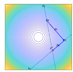
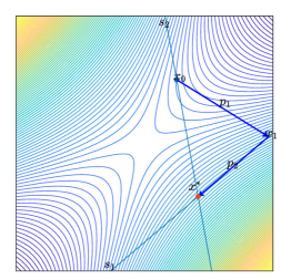
Figure 1: Sketched solutions to saddle systems when $B=I$ (left) or $B=A$ and $A$ is symmetric indefinite.

2.4 Orthogonal updates

We note that when the product ${S}^{\mathrm{\scriptstyle T}}_{k}r_{k-1}$ is a multiple of $e_{k}$, say ${S}^{\mathrm{\scriptstyle T}}_{k}r_{k-1}=\delta_{k}e_{k}$, for some scalar $\delta_{k}$, then the updates $p_{k}$ in (10) are orthogonal with respect to the weighting matrix $W^{-1}=B$:

(12) $${p}^{\mathrm{\scriptstyle T}}_{i}W^{-1}{p}_{j}={p}^{\mathrm{\scriptstyle T}}_{i}B{p}_{j}=0,\quad 1\leq i\leq j\leq k$$

In order to see this orthogonality, suppose $E_{k}=\begin{bmatrix}e_{1}&\cdots&e_{k}\end{bmatrix}$ is the matrix of identity columns, so that $S_{k-1}=S_{k}E_{k-1}$. From (10) this means that $p_{i}\in\text{Range}(WA^{T}S_{k}E_{i})$ and therefore

$$(E^{T}_{i}{S}^{\mathrm{\scriptstyle T}}_{k}AW)W^{-1}{p}_{k}={E}^{\mathrm{\scriptstyle T}}_{i}{S}^{\mathrm{\scriptstyle T}}_{k}{r}_{k-1}=\delta_{k}{E}^{\mathrm{\scriptstyle T}}_{i}{e}_{k}=0,\quad 1\leq i<k.$$

In other words, the updates are orthogonal with respect to the inner product defined by $W^{-1}$, so that (12) is valid.

2.5 PLSS residual

When the sketch consists of previous residuals, i.e., $s_{i}={r}_{i-1}$ for $i=1,2,\ldots,k$ and $B$ is spd, remarkably the update formula (10) simplifies to a short one-step recurrence (we refer to this method as PLSS residual). Further, note that all residuals (with this sketch) are orthogonal. In particular, the residuals satisfy

$${r}_{k}=b-A{x}_{k}=b-A({x}_{k-1}+{p}_{k})={r}_{k-1}-A{p}_{k},$$

and therefore the second block row in (9) results in

(13) $$0={S}_{k}^{T}(A{p}_{k}-{r}_{k-1})=-{S}_{k}^{T}{r}_{k}.$$

As ${S}_{k}=\begin{bmatrix}{r}_{0}\ldots{r}_{k-1}\end{bmatrix}$ contains all previous residuals, (13) implies orthogonality of all residuals. This is an important property of PLSS with residual sketches. For instance, the product ${S}_{k}^{T}{r}_{k-1}$ simplifies to $\|{r}_{k-1}\|^{2}_{2}{e}_{k-1}$. Using this property and further simplifications, we can reduce the explicit formula in (10) to a short recursion ([6, Theorem 1]):

(14) $${p_{k}}={\beta}_{k-1}{p}_{k-1}+{\gamma}_{k-1}W{y}_{k},$$

where

$${y}_{k-1} =A^{\mathrm{\scriptstyle T}}{r}_{k-1}$$

$${\theta}_{k-1} ={p}^{\mathrm{\scriptstyle T}}_{k-1}W^{-1}{p}_{k-1}$$

$${\omega}_{k-1} =\|{r}_{k-1}\|^{2}$$

$${\phi}_{k-1} ={y}^{\mathrm{\scriptstyle T}}_{k}W{y}_{k}$$

$${\beta}_{k-1} =1\big{/}\biggl{(}\frac{{\theta}_{k-1}{\phi}_{k-1}}{{\omega}_{k-1}{\omega}_{k-1}}-1\biggr{)}$$

$${\gamma}_{k-1} =1\big{/}\biggl{(}1-\frac{{\omega}_{k-1}{\omega}_{k-1}}{{\theta}_{k-1}{\phi}_{k-1}}\biggr{)}.$$

Method (14) is extremely efficient compared to the full update formula (10), even though they are mathematically equivalent (modulo that ${S}_{k}$ is based on past residuals).

2.6 PLSS Kaczmarz

A generalization of the randomized Kaczmarz method can be developed from PLSS when the sketching matrix is augmented with one random identity column at each iteration: ${s}_{i_{j}}={e}_{i_{j}}$ for $i_{j}\in\{1,\ldots,m\}$. The sketch is then ${S}_{k}=\begin{bmatrix}{e}_{i_{1}}&\ldots&{e}_{i_{k}}\end{bmatrix}$ and the second block row from (9) implies that ${S}^{\mathrm{\scriptstyle T}}_{k}{r}_{k-1}=({r}_{k-1})_{i_{k}}{e}_{k}$. Using the definition ${\phi}_{i}={p}^{\mathrm{\scriptstyle T}}_{i}W^{-1}{p}_{i}$, we define a diagonal matrix

$${G}_{k}=\textnormal{diag}(\phi_{1},\ldots,{\phi}_{k}).$$

The generalized randomized Kaczmarz method is then given (after simplification of (10)) by the updates [6]

(15) $$p_{k}={\eta}_{k-1}{d}_{k-1},$$

where

$${\eta}_{k-1} =\frac{({r}_{k-1})_{i_{k}}}{a_{i_{k}*}{d}_{k-1}}$$

$${d}_{k-1} =W{y}_{k-1}-{P}_{k-1}G^{-1}_{k-1}P^{T}_{k-1}{y}_{k-1}$$

$${y}_{k-1} =A^{T}{r}_{k-1}.$$

PLSS residual and PLSS Kaczmarz are different methods that result from different choices for the sketch. However, note that the iterations in Eq. 14 or Eq. 15 are still parametrized by the arbitrary symmetric matrix $W$ (and hence $B$).

3 New methods

Here we develop new weighting strategies depending on the properties of $A$. Since $B$ is symmetric, system Eq. 9 corresponds to the first-order optimality conditions of a certain optimization problem. The left plot of Fig. 1 shows the updates generated from a minimization process with an spd $B$, while the right plot corresponds to a symmetric indefinite $B$. Our discussion starts with spd $A$ and least-squares problems before describing symmetric indefinite systems and then general (nonsymmetric) square systems. From now on we use the notation

(16) $$v_{k} :=Ap_{k},\quad u_{k}:=A^{-1}p_{k},\quad y_{k}:=A^{\mathrm{\scriptstyle T}}r_{k},\quad w_{k}:=Wy_{k},$$

$$\theta_{k} ={p}^{\mathrm{\scriptstyle T}}_{k}W^{-1}{p}_{k},\qquad\quad\ \phi_{k}=r_{k}^{\mathrm{\scriptstyle T}}AWA^{\mathrm{\scriptstyle T}}r_{k},$$

$$\beta_{k} =1\big{/}\biggl{(}\frac{\theta_{k}\phi_{k}}{\omega_{k}\omega_{k}}-1\biggr{)},\quad\gamma_{k}=\frac{\theta_{k}}{\omega_{k}}\beta_{k}.$$

3.1 Symmetric positive definite

When $B$ is spd, the $2\times 2$ block system Eq. 9 corresponds to the optimality conditions of the optimization problem

(17) $$\underset{p\in\mathbb{R}^{n}}{\textnormal{ minimize }}\quad\frac{1}{2}p^{\mathrm{\scriptstyle T}}Bp$$

$$\textnormal{ subject to }\>{S}_{k}^{\mathrm{\scriptstyle T}}Ap={S}_{k}^{\mathrm{\scriptstyle T}}{r}_{k-1}.$$

$B=I$ gives the minimum-norm objective $\frac{1}{2}\|p\|^{2}_{2}$. For the solution ${p}_{k}$ to be a global minimizer of (17), $B$ must be positive semidefinite. Further, when $AS_{k}$ and $B$ have full rank, $p_{k}$ is the unique minimizer. When $B$ is any spd matrix, the objective in Eq. 17 can equivalently be written as $\frac{1}{2}\|p\|^{2}_{B}$ (thus $B$ can be interpreted as a weighting). Recall that with a general sketch, the solution of Eq. 9 is given by Eq. 10. However, when previous residuals make up the sketch columns, the update reduces to a short recurrence Eq. 14. If $A$ is spd, we would like to exploit this property. Possible choices for $B$ are $B=A^{-1}$ or $B=A$, which are both spd.

3.1.1 Symmetric positive definite: Method 1

Since $p_{k}$ in recurrence Eq. 14 is expressed in terms of $W=B^{-1}$, an immediate choice of weighting could be $B=A^{-1}$, so that $W=A$. The only difficulty for implementing the recurrence in this case is computing the scalar

$$\theta_{k-1}={p}^{\mathrm{\scriptstyle T}}_{k-1}W^{-1}{p}_{k-1}={p}^{\mathrm{\scriptstyle T}}_{k-1}A^{-1}{p}_{k-1},$$

as it depends on $A^{-1}$ (which is not available). Nevertheless, we can exploit the short recurrence Eq. 14 to deduce a relation for $A^{-1}p_{k}$. Premultiplying

$$p_{k}={\beta}_{k-1}{p}_{k-1}+{\gamma}_{k-1}{w}_{k-1}$$

by $A^{-1}$ and using the notation Eq. 16, we see that $u_{k}=A^{-1}p_{k}$ satisfies

$${u}_{k}={\beta}_{k-1}{u}_{k-1}+{\gamma}_{k-1}{y}_{k-1}.$$

With this relation a short recursive algorithm can be developed that does not require any computations with $A^{-1}$. This method is based on residuals for the sketch; hence it derives from the relations in Eq. 14. Second, we specify the arbitrary weight to ne $B=A^{-1}$ and ensure that all scalars in Eq. 16 can be computed.

Algorithm 1: PLSS (spd $B=A^{-1}$)
Given: $r_{0}=b-Ax_{0};\quad y_{0}=A^{\mathrm{\scriptstyle T}}r_{0};\quad w_{0}=Ay_{0}$
$\omega_{0}=\|r_{0}\|^{2};\quad\phi_{0}=y_{0}^{\mathrm{\scriptstyle T}}w_{0};\quad u_{1}=(\omega_{0}/\phi_{0})y_{0};\quad p_{1}=(\omega_{0}/\phi_{0})w_{0}$
$x_{1}=x_{0}+p_{1};\quad r_{1}=b-Ax_{1};\quad y_{1}=A^{\mathrm{\scriptstyle T}}r_{1};\quad w_{1}=Ay_{1}$
for $k=2,3,\dots,n$
	${\theta}_{k-1}={p}^{\mathrm{\scriptstyle T}}_{k-1}{u}_{k-1};\quad{\phi}_{k-1}={y}^{\mathrm{\scriptstyle T}}_{k-1}{w}_{k-1}$
	${\omega}_{k-1}=\|{r}_{k-1}\|^{2}$
	${\beta}_{k-1}=1\big{/}\big{(}\frac{{\theta}_{k-1}{\phi}_{k-1}}{{\omega}_{k-1}{\omega}_{k-1}}-1\big{)}$
	${\gamma}_{k-1}=\frac{{\theta}_{k-1}}{{\omega}_{k-1}}{\beta}_{k-1}$
	$u_{k}={\beta}_{k-1}{u}_{k-1}+{\gamma}_{k-1}{y}_{k-1}$
	$p_{k}={\beta}_{k-1}{p}_{k-1}+{\gamma}_{k-1}{w}_{k-1}$
	$x_{k}={x}_{k-1}+p_{k}$
	$r_{k}=b-Ax_{k}$
	$y_{k}=A^{\mathrm{\scriptstyle T}}r_{k}$
	$w_{k}=Ay_{k}$
end

A few notes about Algorithm 1. First, it is designed for symmetric $A$ and therefore any occurrences of $A^{\mathrm{\scriptstyle T}}$ can be replaced by $A$. Second, it has low memory usage: only 6 vectors of size $n$ are being updated. Third, it is computationally efficient, especially compared to randomized algorithms that compute the update via Eq. 10 (see [11, 16]). Compared to other iterative methods it is moderately efficient in using three matvec operations per iteration. Also, it possesses the finite termination property because the sketch consists of the history of residuals, by virtue of its derivation from (14).

3.1.2 Symmetric positive definite: Method 2

We can develop a second algorithm by choosing $B=A$ so that $W=A^{-1}$. At first this choice seems to make recursion Eq. 14 difficult to compute because the vector

$${w}_{k-1}=W{y}_{k-1}=A^{-1}{y}_{k-1}$$

is needed in the update. However, when $A$ is symmetric we have

$${w}_{k-1}=A^{-1}{y}_{k-1}=A^{-1}(A^{\mathrm{\scriptstyle T}}{r}_{k-1})={r}_{k-1}.$$

In other words, the computations with the inverse cancel out. The scalars can also be computed directly:

$${\theta}_{k-1}={p}^{\mathrm{\scriptstyle T}}_{k-1}W^{-1}{p}_{k-1}={p}^{\mathrm{\scriptstyle T}}_{k-1}{v}_{k-1}\quad\text{ and }\quad{\phi}_{k-1}={y}^{\mathrm{\scriptstyle T}}_{k-1}W{y}_{k-1}={r}^{\mathrm{\scriptstyle T}}_{k-1}{y}_{k-1},$$

where $v_{k}=Ap_{k}$. Because $p_{k}$ satisfies

$$p_{k}={\beta}_{k-1}{p}_{k-1}+{\gamma}_{k-1}{r}_{k-1},$$

$v_{k}$ can be found to follow the relation

$$v_{k}={\beta}_{k-1}{v}_{k-1}+{\gamma}_{k-1}{y}_{k-1}.$$

The algorithm using this weighting follows.

Algorithm 2: PLSS (spd $B=A$)
Given: $r_{0}=b-Ax_{0};\quad y_{0}=A^{\mathrm{\scriptstyle T}}r_{0};$
$\omega_{0}=\|r_{0}\|^{2};\quad\phi_{0}=y_{0}^{\mathrm{\scriptstyle T}}r_{0};\quad p_{1}=(\omega_{0}/\phi_{0})r_{0};\quad v_{1}=Ap_{1}$
$x_{1}=x_{0}+p_{1};\quad r_{1}=r_{0}-v_{1};\quad y_{1}=A^{\mathrm{\scriptstyle T}}r_{1};$
for $k=2,3,\dots,n$
	${\theta}_{k-1}={p}^{\mathrm{\scriptstyle T}}_{k-1}{v}_{k-1};\quad{\phi}_{k-1}={y}^{\mathrm{\scriptstyle T}}_{k-1}{r}_{k-1}$
	${\omega}_{k-1}=\|{r}_{k-1}\|^{2}$
	${\beta}_{k-1}=1\big{/}\big{(}\frac{{\theta}_{k-1}{\phi}_{k-1}}{{\omega}_{k-1}{\omega}_{k-1}}-1\big{)}$
	${\gamma}_{k-1}=\frac{{\theta}_{k-1}}{{\omega}_{k-1}}{\beta}_{k-1}$
	$v_{k}={\beta}_{k-1}{v}_{k-1}+{\gamma}_{k-1}{y}_{k-1}$
	$p_{k}={\beta}_{k-1}{p}_{k-1}+{\gamma}_{k-1}{r}_{k-1}$
	$x_{k}={x}_{k-1}+p_{k}$
	$r_{k}={r}_{k-1}-v_{k}$
	$y_{k}=A^{\mathrm{\scriptstyle T}}r_{k}$
end

As before, $A^{\mathrm{\scriptstyle T}}$ can be replaced by $A$. The memory footprint is low (storing and updating only five vectors), and importantly, the algorithm is very efficient: each iteration needs only one matvec operation, ${y}_{k}=A^{\mathrm{\scriptstyle T}}r_{k}$. Again the method enjoys finite termination. Finally, the residuals generated by this algorithm are equivalent to those from CG [12].

3.1.3 Comparison: Symmetric positive definite

Detailed comparisons of various methods are reported in Section 4 (Numerical Experiments). Here we provide some intuition on the efficacy of the previous algorithms. We include a regular randomized method, where the sketch $S_{k}\in\mathbb{R}^{n\times r}$ is computed as a standard normal random matrix and the update is obtained by explicitly evaluating Eq. 10 with $W=I$. The algorithms are applied on a small spd matrix with $n=10$. The size for the random sketch is $r=n/2=5$, and all methods are initialized with the same zero vector $x_{0}=0$. The results are in Table 1. We make a few observations about the table. First note the finite termination property. PLSS with residual sketches has finite termination, because all residuals are orthogonal by construction. The methods converge to the solution in at most $n$ iterations. One can see this taking effect for $k=10=n$, where the residual norms drop rapidly to convergence tolerances. In contrast, the iteration with random normal sketches converges based on a rate and typically converges much slower in practice. Further, the computational costs of the PLSS algorithms are very low because of the short recurrences. On the other hand, the standard Randn algorithm needs to perform updates via the costly formula Eq. 10. Finally, PLSS ($B=A$) tends to converge much more rapidly than PLSS ($B=A^{-1}$). Since PLSS ($B=A$) uses only one matrix-vector multiply per iteration as opposed to three for PLSS ($B=A^{-1}$), we view the former as the better of the two.

Table 1: Residual norms of three algorithms for a $10\times 10$ spd system.

$k$	$\|r_{k}\|_{2}$
	Randn.	PLSS ($B=A^{-1}$)	PLSS ($B=A$)
0	4.1653e+04	4.1653e+04	4.1653e+04
1	1.5470e+04	1.3794e+04	6.6381e+03
2	1.0068e+04	1.5185e+04	1.1624e+03
3	6.9911e+03	3.9838e+03	3.2431e+02
4	2.9346e+03	2.6166e+03	7.5577e+01
5	1.8590e+03	1.4479e+03	1.6274e+01
6	1.3115e+03	9.2966e+02	1.7461e+00
7	1.0382e+03	3.0200e+02	2.3732e-01
8	1.0255e+03	9.5402e+01	2.1046e-02
9	7.0308e+02	2.2631e+01	1.5050e-03
10	6.9981e+02	2.2689e-09	3.1511e-16

3.2 Least squares

When problem Eq. 1 is overdetermined with $m>n$, the system is typically inconsistent. To find the least-squares solution we have to solve $A^{\mathrm{\scriptstyle T}}Ax=A^{\mathrm{\scriptstyle T}}b$. A simple and often effective approach is to apply Algorithm 2, i.e., PLSS ($W=\widehat{A}$) with $\widehat{A}=A^{\mathrm{\scriptstyle T}}A$ and $\widehat{b}=A^{\mathrm{\scriptstyle T}}b$. Recall that Algorithm 2 uses only one matvec with $\widehat{A}$ per iteration, which can be implemented as two products with $A$. In particular, the product $\widehat{A}r$ (for some $r\in\mathbb{R}^{n}$) is implemented as $\widehat{A}r=A^{\mathrm{\scriptstyle T}}(Ar)$.

3.3 Symmetric indefinite

When $B$ is symmetric but indefinite, the block system Eq. 9 still characterizes the critical points of an optimization problem. However, the objective $\frac{1}{2}p^{\mathrm{\scriptstyle T}}Bp$ is not a norm anymore because it can assume negative values. Therefore, the solution to Eq. 9 is typically not the minimizer. (This is good because the minimizer is typically unbounded.) Broadly, $p_{k}$ in this context is related to a saddle point in a quadratic programming problem. For an example, one can compare the updates generated with an indefinite weighting $B$ in Fig. 1. Independent of everything else, as long as the sketch remains full-rank, finite termination is maintained (even with indefinite $B$). Because $p_{k}$ can’t be interpreted as a minimizer in the indefinite case, we develop the update using an analogy to spd $B$. We view $B$ as an implicit preconditioner with the main purpose of simplifying computations. Recall the short recurrence Eq. 14 for the update with residual sketches (independent of the definiteness of $B$). Since

$$W{y}_{k-1}=WA^{\mathrm{\scriptstyle T}}{r}_{k-1}=WA{r}_{k-1},$$

a significant simplification occurs when $W=A^{-1}$ so that $W{y}_{k-1}={r}_{k-1}$. This means we choose $B=A$, even if $A$ is indefinite. The result is an algorithm that is computationally equivalent to Algorithm 2. We summarize the method as follows.

Algorithm 3: PLSS (sid $B=A$)

Given: $r_{0}=b-Ax_{0};\quad y_{0}=A^{\mathrm{\scriptstyle T}}r_{0}$

Apply Algorithm 2

Note that Algorithm 2 (and hence Algorithm 3) does not require any square roots, and thus there is no concern about square roots of negative quantities in the indefinite case causing breakdown. Since $\omega_{k-1}=0$ appears in the denominator, we potentially have to guard for this value becoming too small. However, $\omega_{k-1}=0$ implies ${r}_{k-1}=0$ and therefore this quantity is small only when the method has converged. Further, the denominator in $\beta_{k-1}$ must be guarded from becoming zero. With $W=A^{-1}$ in $\beta_{k-1}$ from Algorithm 2 (and the notation Eq. 16) we see that

$$\beta_{k-1}=\frac{1}{\frac{{\theta}_{k-1}{\phi}_{k-1}}{{\omega}_{k-1}{\omega}_{k-1}}-1}=\frac{1}{\frac{({p}^{\mathrm{\scriptstyle T}}_{k-1}A{p}_{k-1})({r}^{\mathrm{\scriptstyle T}}_{k-1}A{r}_{k-1})}{\|{r}_{k-1}\|^{4}}-1}.$$

The denominator is zero if $({p}^{\mathrm{\scriptstyle T}}_{k-1}A{p}_{k-1})({r}^{\mathrm{\scriptstyle T}}_{k-1}A{r}_{k-1})=\|{r}_{k-1}\|^{4}$.

A possible remedy is to restart the method from ${x}_{k-1}$ should this condition arise. (In the numerical experiments we don’t observe breakdowns from this condition.) Algorithm 3 is efficient because it uses only one matvec per iteration. It is equivalent to CG but applicable to symmetric indefinite systems, whereas CG is typically designed for spd matrices. In Section 4.1 (Experiment I: Indefinite Systems) we observe that PLSS ($B=A$) (Algorithm 3) is robust and fast (see Tables 2 and 3).

3.4 General square systems

When $A$ is square, we can’t directly apply the strategies for $B$ from Sections 3.1 and 3.3. Specifically, it is not possible to choose $B=A$ or $B=A^{-1}$ as before because $A$ is not necessarily symmetric. It is fine to set $B=I$, which results in the original PLSS algorithm. Another approach is to consider the symmetric weighting $B=A^{\mathrm{\scriptstyle T}}A$. Substituting $W=B^{-1}$ in the update Eq. 8 (with residual sketches), we obtain

$${p}_{k}=A^{-1}{S}_{k}({S}^{\mathrm{\scriptstyle T}}_{k}{S}_{k})^{-1}{S}_{k}{r}_{k-1}=A^{-1}{r}_{k-1}.$$

The main difficulty is evaluating $A^{-1}{r}_{k-1}$. In fact, if $A^{-1}r_{0}$ could be computed exactly the method based on this choice for $B$ would converge in one iteration:

$$p_{1}=A^{-1}r_{0}=A^{-1}b-x_{0},\quad\text{ and }\quad x_{1}=x_{0}+p_{1}=A^{-1}b.$$

However, $A^{-1}{r}_{k-1}$ is typically not computed exactly. A possibility is to apply PLSS ($B=I$) as a subproblem solver inside an outer loop in order to evaluate $A^{-1}{r}_{k-1}$ approximately. This approach has two nested loops and we don’t want the inner loop to take many iterations. Therefore, we include a second stopping tolerance $\epsilon_{k}=\|r_{k}\|\big{/}k$ to terminate the inner loop early. The resulting Algorithm 4 uses PLSS ($B=I$) represented as the function in Fig. 2 with its own stopping tolerance $\epsilon_{0}$.

function plss($x_{0},b,A,\epsilon$)
$r_{0}=b-Ax_{0};\quad y_{0}=A^{\mathrm{\scriptstyle T}}r_{0};$
$\omega_{0}=\|r_{0}\|^{2};\quad\phi_{0}=\|y_{0}\|^{2};\quad p_{1}=(\omega_{0}/\phi_{0})y_{0};\quad v_{1}=Ap_{1}$
$x_{1}=x_{0}+p_{1};\quad r_{1}=r_{0}-v_{1};\quad y_{1}=A^{\mathrm{\scriptstyle T}}r_{1};k=2;$
while $\|{r}_{k-1}\|>\epsilon$
	${\theta}_{k-1}=\|{p}_{k-1}\|^{2};\quad{\phi}_{k-1}=\|{y}_{k-1}\|^{2}$
	${\omega}_{k-1}=\|{r}_{k-1}\|^{2}$
	${\beta}_{k-1}=1\big{/}\big{(}\frac{{\theta}_{k-1}{\phi}_{k-1}}{{\omega}_{k-1}{\omega}_{k-1}}-1\big{)}$
	${\gamma}_{k-1}=\frac{{\theta}_{k-1}}{{\omega}_{k-1}}{\beta}_{k-1}$
	$p_{k}={\beta}_{k-1}{p}_{k-1}+{\gamma}_{k-1}{r}_{k-1}$
	$v_{k}=Ap_{k}$
	$x_{k}={x}_{k-1}+p_{k}$
	$r_{k}={r}_{k-1}-v_{k}$
	$y_{k}=A^{\mathrm{\scriptstyle T}}r_{k}$
	$k=k+1$
end

Figure 2: Function plss.

Algorithm 4: PLSS (general $B=A^{\mathrm{\scriptstyle T}}A$)
Given: $r_{0}=b-Ax_{0};\quad y_{0}=A^{\mathrm{\scriptstyle T}}r_{0};\quad\epsilon_{0}>0$
Solve $Ap_{1}=r_{0}$ using plss($0,b,A,\epsilon_{0}$)
$x_{1}=x_{0}+p_{1}$
for $k=2,3,\dots,k_{\text{max}}$
	${r}_{k-1}=b-A{x}_{k-1}$
	Solve $Ap_{k}={r}_{k-1}$ using plss($\frac{8}{10}{p}_{k-1},{r}_{k-1},A,\frac{\|{r}_{k-1}\|}{k-1}$) in Fig. 2
	$x_{k}={x}_{k-1}+p_{k}$
end

A few remarks about Algorithm 4. First, inside the loop, plss is called with an initial guess of $\frac{8}{10}{p}_{k-1}$. This is not essential, and the zero starting point is a valid option. However, when the residuals don’t change rapidly for every iteration it can be advantageous to use information from the previous solution. The tolerances $\epsilon_{k}=\frac{\|{r}_{k-1}\|}{k-1}$ are only one implementation that force increasingly accurate solutions. Other sequences are possible. Further, if PLSS ($B=I$) could solve the initial system $Ap_{1}=r_{0}$ to full accuracy, Algorithm 4 would only need one iteration. However, as this is unrealistic, the algorithm will typically use multiple iterations and its convergence depends on how well the subproblem solver approximates $Ap_{k}={r}_{k-1}$. When matvec products with $A$ can be computed cheaply, the overall approach in Algorithm 4 can be useful. Numerical experiments for general square $A$ are in Section 4.2.

4 Numerical experiments

Our algorithms are implemented in MATLAB and PYTHON 3.9. The numerical experiments are carried out in MATLAB 2023a on a Linux machine with Intel 13th Gen Intel Core i9-13900KS (24 cores) processor and 128 GB RAM and a laptop with Apple M2 Max chip. For comparisons, we use randomized algorithms of [11], the Algorithms from [6, github.com/johannesbrust/PLSS], SYMMLQ [15] and GMRES [18]. All codes are available in the public domain [3]. The stopping criterion is either $\|{A}{x}_{k}-b\|_{2}/\|b\|_{2}\leq\epsilon$. Unless otherwise specified, the iteration limit is $n$. We label the PLSS Algorithm with ${B}={I}$ and $B=\text{diag}(\|a_{1}\|,\dots,\|a_{n}\|)$ as PLSS $(B=I)$ and PLSS $(B=\text{Diag.})$ respectively.

4.1 Experiment I

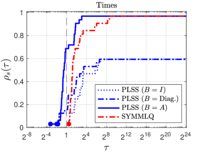
Figure 3: Computational times of the four solvers on 32 square symmetric indefinite matrices from SuiteSparse.

The problems in this experiment are large square consistent symmetric systems. However, the matrices may be indefinite and/or rank-deficient. For example, problem bcsstm36 is neither positive definite nor full-rank. The convergence criterion is $\epsilon=1\times 10^{-4}$ and the iterations limit is set to $\textnormal{maxit}=\textnormal{round}(\frac{11}{10}n)$. Table 2 gives a detailed comparison of the solver outcomes. We note that PLSS with weighting $B=A$ and SYMMLQ solve all but one problem to the specified tolerance. In terms of computational time, PLSS with the new weighting is the fastest overall. Fig. 3 summarizes the computational times of the four methods using performance profiles [9]. These profiles allow for a direct comparison of different solver based on computational times or iterations. Specifically, the performance metric $\rho_{s}(\tau)$ on $n_{p}$ test problems is given by

$$\rho_{s}(\tau)=\frac{\text{card}\left\{p:\pi_{p,s}\leq\tau\right\}}{n_{p}}\quad\text{and}\quad\pi_{p,s}=\frac{t_{p,s}}{\underset{1\leq i\leq S,\ i\neq s}{\text{ min }t_{p,i}}},$$

where $t_{p,s}$ is the “output” (i.e., iterations or time) of “solver” $s$ on problem $p$, and $S$ denotes the total number of solvers for a given comparison. This metric measures the proportion of how close a given solver is to the best result.

Table 2: Experiment I compares 4 solvers on 32 linear systems from the SuiteSparse Matrix Collection [8] with stopping tolerance $\epsilon=10^{-4}$ and iteration limit $\frac{11}{10}n$. In column 3, “Dty” is the density of a particular matrix $A$ calculated as $\text{Dty}=\frac{\text{nnz}(A)}{n\cdot n}$. Entries with superscript ^† denote problems for which the solver did not converge to the specified tolerance. Bold entries mark the fastest times, while second fastest times are italicized.

Problem $n$ Dty PLSS ($B=I$) PLSS ($B=\text{Diag.}$) PLSS ($B=A$) SYMMLQ [15] It Sec Res It Sec Res It Sec Res It Sec Res bcspwr10 5300 0.0008 1378 0.17 0.0001 529 0.076 0.0001 1904 0.06 0.0001 1734 0.16 9e-05 bcsstk17 10974 0.004 $\textnormal{12071}^{\dagger}$ $\textnormal{5.1}^{\dagger}$ $\textnormal{0.03}^{\dagger}$ $\textnormal{12071}^{\dagger}$ $\textnormal{5.4}^{\dagger}$ $\textnormal{0.03}^{\dagger}$ 1984 0.36 9e-05 1926 0.72 9e-05 bcsstk18 11948 0.001 $\textnormal{13143}^{\dagger}$ $\textnormal{4.4}^{\dagger}$ $\textnormal{0.003}^{\dagger}$ $\textnormal{13143}^{\dagger}$ $\textnormal{4.5}^{\dagger}$ $\textnormal{0.003}^{\dagger}$ 603 0.096 9e-05 593 0.16 0.0001 bcsstk25 15439 0.001 $\textnormal{16983}^{\dagger}$ $\textnormal{7.1}^{\dagger}$ $\textnormal{0.0005}^{\dagger}$ $\textnormal{16983}^{\dagger}$ $\textnormal{7.5}^{\dagger}$ $\textnormal{0.0005}^{\dagger}$ 254 0.06 0.0001 247 0.1 9e-05 bcsstk29 13992 0.003 1372 0.82 0.0001 193 0.12 0.0001 1358 0.37 0.0001 1245 0.65 0.0001 bcsstk30 28924 0.002 1934 3.6 0.0001 194 0.36 9e-05 1859 1 0.0001 1524 2.2 0.0001 bcsstk31 35588 0.0009 2408 2.7 0.0001 236 0.28 0.0001 2370 0.94 0.0001 2007 2 0.0001 bcsstk32 44609 0.001 2102 3.8 0.0001 231 0.43 9e-05 2206 1.2 0.0001 1818 2.7 0.0001 bcsstk33 8738 0.008 1127 0.55 0.0001 456 0.22 9e-05 1199 0.19 9e-05 1097 0.44 0.0001 bcsstm25 15439 6e-05 9844 2.1 9e-05 1161 0.29 6e-05 162 0.029 6e-05 157 0.04 7e-05 bcsstk35 30237 0.002 $\textnormal{33261}^{\dagger}$ $\textnormal{45}^{\dagger}$ $\textnormal{0.005}^{\dagger}$ $\textnormal{33261}^{\dagger}$ $\textnormal{49}^{\dagger}$ $\textnormal{0.003}^{\dagger}$ 674 0.36 0.0001 660 0.83 0.0001 bcsstk36 23052 0.002 $\textnormal{25357}^{\dagger}$ $\textnormal{27}^{\dagger}$ $\textnormal{0.02}^{\dagger}$ $\textnormal{25357}^{\dagger}$ $\textnormal{28}^{\dagger}$ $\textnormal{0.02}^{\dagger}$ 1800 0.8 0.0001 1735 1.7 0.0001 bcsstk37 25503 0.002 $\textnormal{28053}^{\dagger}$ $\textnormal{31}^{\dagger}$ $\textnormal{0.04}^{\dagger}$ $\textnormal{28053}^{\dagger}$ $\textnormal{32}^{\dagger}$ $\textnormal{0.03}^{\dagger}$ 1639 0.78 0.0001 1623 1.6 0.0001 bcsstk38 8032 0.006 $\textnormal{8835}^{\dagger}$ $\textnormal{3.1}^{\dagger}$ $\textnormal{0.0002}^{\dagger}$ $\textnormal{8835}^{\dagger}$ $\textnormal{3.1}^{\dagger}$ $\textnormal{0.0002}^{\dagger}$ 58 0.0085 9e-05 55 0.015 0.0001 bcsstm35 30237 2e-05 5783 2.7 9e-05 5703 3.2 0.0001 89 0.033 9e-05 223 0.11 6e-06 bcsstm36 23052 0.0006 $\textnormal{25357}^{\dagger}$ $\textnormal{15}^{\dagger}$ $\textnormal{0.0002}^{\dagger}$ $\textnormal{25357}^{\dagger}$ $\textnormal{17}^{\dagger}$ $\textnormal{0.0002}^{\dagger}$ 138 0.06 9e-05 137 0.094 9e-05 bcsstm37 25503 2e-05 81 0.034 0.0001 81 0.039 0.0001 9 0.0036 8e-05 74 0.036 5e-07 bcsstm38 8032 0.0002 1187 0.17 9e-05 673 0.094 0.0001 24 0.0015 9e-05 22 0.0029 9e-05 bcsstm39 46772 2e-05 5023 2.7 0.0001 290 0.2 9e-05 128 0.052 0.0001 137 0.08 0.0001 crystk02 13965 0.005 0 0.00084 6e-11 0 0.0024 6e-11 0 0.0027 6e-11 370 0.25 6e-15 crystk03 24696 0.003 0 0.0013 4e-11 0 0.0048 4e-11 0 0.0047 4e-11 389 0.52 4e-15 crystm02 13965 0.002 0 0.00035 1e-10 0 0.001 1e-10 0 0.0029 1e-10 35 0.018 1e-14 crystm03 24696 0.001 0 0.00044 1e-10 0 0.0017 1e-10 0 0.0025 1e-10 35 0.029 1e-14 ct20stif 52329 0.0009 $\textnormal{57562}^{\dagger}$ $\textnormal{1.4e+02}^{\dagger}$ $\textnormal{0.0002}^{\dagger}$ $\textnormal{57562}^{\dagger}$ $\textnormal{1.5e+02}^{\dagger}$ $\textnormal{0.0002}^{\dagger}$ 338 0.25 0.0001 281 0.59 0.0001 msc10848 10848 0.01 55 0.072 7e-05 54 0.069 8e-05 28 0.011 6e-05 25 0.021 8e-05 msc23052 23052 0.002 $\textnormal{25357}^{\dagger}$ $\textnormal{31}^{\dagger}$ $\textnormal{0.02}^{\dagger}$ $\textnormal{25357}^{\dagger}$ $\textnormal{32}^{\dagger}$ $\textnormal{0.02}^{\dagger}$ 1838 0.86 9e-05 1724 1.9 0.0001 pcrystk02 13965 0.005 907 0.69 0.0001 362 0.27 0.0001 900 0.21 0.0001 742 0.44 0.0001 pcrystk03 24696 0.003 707 1.2 0.0001 262 0.45 9e-05 678 0.36 9e-05 560 0.81 0.0001 pct20stif 52329 0.001 2511 6.3 0.0001 476 1.3 0.0001 2301 1.7 0.0001 1816 3.9 0.0001 mplate 5962 0.004 $\textnormal{6558}^{\dagger}$ $\textnormal{6.5}^{\dagger}$ $\textnormal{0.1}^{\dagger}$ $\textnormal{6558}^{\dagger}$ $\textnormal{7.3}^{\dagger}$ $\textnormal{0.2}^{\dagger}$ $\textnormal{6558}^{\dagger}$ $\textnormal{{2.9}}^{\dagger}$ $\textnormal{0.06}^{\dagger}$ $\textnormal{5712}^{\dagger}$ $\textnormal{\emph{5.2}}^{\dagger}$ $\textnormal{5e+02}^{\dagger}$ vibrobox 12328 0.002 $\textnormal{13561}^{\dagger}$ $\textnormal{5.4}^{\dagger}$ $\textnormal{0.001}^{\dagger}$ $\textnormal{13561}^{\dagger}$ $\textnormal{5.6}^{\dagger}$ $\textnormal{0.001}^{\dagger}$ 268 0.053 9e-05 263 0.089 9e-05 ex15 6867 0.002 $\textnormal{7554}^{\dagger}$ $\textnormal{1.3}^{\dagger}$ $\textnormal{0.007}^{\dagger}$ $\textnormal{7554}^{\dagger}$ $\textnormal{1.4}^{\dagger}$ $\textnormal{0.006}^{\dagger}$ 627 0.057 0.0001 619 0.08 0.0001

4.2 Experiment II

The problems in this experiment medium size are general square systems. The convergence tolerance is $\epsilon=1\times 10^{-4}$ and the iteration limit is $\textnormal{maxit}=n$. Table 3 gives a detailed comparison of the solver outcomes. PLSS with weighting $B=A^{\mathrm{\scriptstyle T}}A$ solves the most problems to the specified tolerance. For reference we include GMRES [18] with restarts every 500 iterations. Figure 4 summarizes the computational times of the four methods.

Table 3: Experiment II compares 4 solvers on 19 general square systems from the SuiteSparse Matrix Collection [8] with stopping tolerance $\epsilon=10^{-4}$ and iteration limit $n$. In column 3, “Dty” is the density of a particular matrix $A$ calculated as $\text{Dty}=\frac{\text{nnz}(A)}{n\cdot n}$. Entries with superscript ^† denote problems for which the solver did not converge to the specified tolerance. Bold entries mark the fastest times, while second fastest times are italicized.

Problem $n$ Dty PLSS ($B=I$) PLSS ($B=\text{Diag.}$) PLSS ($B=A^{\mathrm{\scriptstyle T}}A$) GMRES [18] It Sec Res It Sec Res It Sec Res It Sec Res gemat11 4929 0.001 $\textnormal{4929}^{\dagger}$ $\textnormal{{0.7}}^{\dagger}$ $\textnormal{0.007}^{\dagger}$ $\textnormal{4929}^{\dagger}$ $\textnormal{\emph{0.75}}^{\dagger}$ $\textnormal{0.003}^{\dagger}$ 44 22 9e-05 $\textnormal{5500}^{\dagger}$ $\textnormal{55}^{\dagger}$ $\textnormal{0.3}^{\dagger}$ gemat12 4929 0.001 $\textnormal{4929}^{\dagger}$ $\textnormal{{0.68}}^{\dagger}$ $\textnormal{0.002}^{\dagger}$ $\textnormal{4929}^{\dagger}$ $\textnormal{\emph{0.74}}^{\dagger}$ $\textnormal{0.0007}^{\dagger}$ 23 9.5 9e-05 $\textnormal{5500}^{\dagger}$ $\textnormal{55}^{\dagger}$ $\textnormal{0.05}^{\dagger}$ gre_1107 1107 0.005 795 0.011 9e-05 770 0.012 9e-05 7 0.023 2e-05 $\textnormal{1500}^{\dagger}$ $\textnormal{0.46}^{\dagger}$ $\textnormal{0.02}^{\dagger}$ lns_3937 3937 0.002 $\textnormal{3937}^{\dagger}$ $\textnormal{{0.19}}^{\dagger}$ $\textnormal{0.04}^{\dagger}$ $\textnormal{3937}^{\dagger}$ $\textnormal{\emph{0.22}}^{\dagger}$ $\textnormal{0.05}^{\dagger}$ 225 37 0.0001 $\textnormal{4500}^{\dagger}$ $\textnormal{11}^{\dagger}$ $\textnormal{0.07}^{\dagger}$ lnsp3937 3937 0.002 $\textnormal{3937}^{\dagger}$ $\textnormal{{0.2}}^{\dagger}$ $\textnormal{0.05}^{\dagger}$ $\textnormal{3937}^{\dagger}$ $\textnormal{\emph{0.23}}^{\dagger}$ $\textnormal{0.04}^{\dagger}$ $\textnormal{3937}^{\dagger}$ $\textnormal{89}^{\dagger}$ $\textnormal{0.007}^{\dagger}$ $\textnormal{4500}^{\dagger}$ $\textnormal{12}^{\dagger}$ $\textnormal{0.07}^{\dagger}$ mahindas 1258 0.005 3 0.0079 8e-05 3 0.013 2e-05 2 0.014 4e-05 517 0.009 0.0001 nnc1374 1374 0.005 $\textnormal{1374}^{\dagger}$ $\textnormal{\emph{0.024}}^{\dagger}$ $\textnormal{0.0002}^{\dagger}$ 1107 0.021 0.0001 11 0.11 9e-05 959 0.24 0.0001 orani678 2529 0.01 1864 0.19 9e-05 778 0.084 0.0001 10 0.48 1e-06 $\textnormal{3000}^{\dagger}$ $\textnormal{2.5}^{\dagger}$ $\textnormal{0.4}^{\dagger}$ orsirr_1 1030 0.006 $\textnormal{1030}^{\dagger}$ $\textnormal{{0.012}}^{\dagger}$ $\textnormal{0.01}^{\dagger}$ $\textnormal{1030}^{\dagger}$ $\textnormal{\emph{0.014}}^{\dagger}$ $\textnormal{0.009}^{\dagger}$ 96 0.99 4e-05 674 0.029 9e-05 orsreg_1 2205 0.003 1977 0.045 9e-05 $\textnormal{2205}^{\dagger}$ $\textnormal{0.056}^{\dagger}$ $\textnormal{0.0001}^{\dagger}$ 7 0.15 5e-06 541 0.005 0.0001 plsk1919 1919 0.003 $\textnormal{1919}^{\dagger}$ $\textnormal{{0.035}}^{\dagger}$ $\textnormal{0.0003}^{\dagger}$ $\textnormal{1919}^{\dagger}$ $\textnormal{\emph{0.039}}^{\dagger}$ $\textnormal{0.0006}^{\dagger}$ 10 0.12 7e-05 $\textnormal{2500}^{\dagger}$ $\textnormal{1.5}^{\dagger}$ $\textnormal{0.0002}^{\dagger}$ pores_2 1224 0.006 $\textnormal{1224}^{\dagger}$ $\textnormal{\emph{0.019}}^{\dagger}$ $\textnormal{0.0004}^{\dagger}$ $\textnormal{1224}^{\dagger}$ $\textnormal{0.022}^{\dagger}$ $\textnormal{0.0001}^{\dagger}$ 8 0.064 8e-05 552 0.0044 0.0001 psmigr_1 3140 0.06 $\textnormal{3140}^{\dagger}$ $\textnormal{1.3}^{\dagger}$ $\textnormal{0.001}^{\dagger}$ 90 0.04 0.0001 16 13 9e-05 578 0.053 0.0001 psmigr_2 3140 0.05 684 0.28 0.0001 672 0.29 0.0001 8 2.3 3e-06 $\textnormal{3500}^{\dagger}$ $\textnormal{8.3}^{\dagger}$ $\textnormal{0.01}^{\dagger}$ psmigr_3 3140 0.06 11 0.0052 6e-05 69 0.032 7e-05 5 0.017 8e-06 505 0.0036 7e-05 sherman2 1080 0.02 515 0.013 5e-05 515 0.014 7e-05 9 0.067 2e-05 692 0.038 9e-05 sherman3 5005 0.0008 $\textnormal{5005}^{\dagger}$ $\textnormal{{0.67}}^{\dagger}$ $\textnormal{1}^{\dagger}$ $\textnormal{5005}^{\dagger}$ $\textnormal{\emph{0.71}}^{\dagger}$ $\textnormal{1}^{\dagger}$ $\textnormal{5005}^{\dagger}$ $\textnormal{23}^{\dagger}$ $\textnormal{1}^{\dagger}$ 1128 6 0.0001 sherman4 1104 0.003 867 0.017 0.0001 464 0.017 7e-05 10 0.05 1e-06 585 0.015 9e-05 sherman5 3312 0.002 $\textnormal{3312}^{\dagger}$ $\textnormal{{0.14}}^{\dagger}$ $\textnormal{0.005}^{\dagger}$ $\textnormal{3312}^{\dagger}$ $\textnormal{\emph{0.15}}^{\dagger}$ $\textnormal{0.004}^{\dagger}$ $\textnormal{3312}^{\dagger}$ $\textnormal{94}^{\dagger}$ $\textnormal{0.0003}^{\dagger}$ 1122 1.3 0.0001

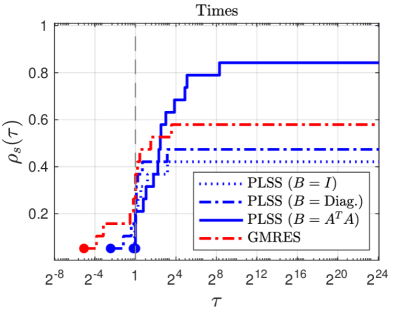
Figure 4: Computational times of the four solvers on 19 general square matrices from SuiteSparse.

4.3 Experiment III

This experiment tests Algorithm 4 on a difficult unsymmetric matrix (West0479) [8] for iterative solvers, when no preconditioner is used. The matrix comes from a chemical engineering process via A. Westerberg. Even though the system is small ($n=479$), the condition number is large: $\kappa(A)\approx 10^{12}$.

For comparison, we include three random normal solvers with $r=50,100,150$. We run Algorithm 4 with inner iterations limit $10n$. The convergence tolerance for all methods is $\epsilon=10^{-6}$. As Algorithm 4 has cheap inner and costly outer iterations, a comparison based on iterations only may not be informative. Instead we compare computation times. Figure 5 shows the outcomes. We see that Rand $(r=150)$ and Algorithm 4 (PLSS with $B=A^{\mathrm{\scriptstyle T}}A$) perform well. Importantly, Algorithm 4 scales to larger problems because the subproblem solver has low inner iterations complexity. Every iteration of the randomized algorithm needs $O(r^{3})$ operations.

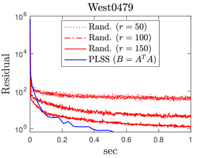
Figure 5: Computational times of four solvers on the West0479 matrix.

5 Conclusion

Structured sketch-and-project methods for linear systems have been developed here. The methods are characterized by a finite termination property for both random and deterministic sketches. When the history of past residuals forms the sketch, we exploit a short recurrence to develop effective weighting schemes. The techniques enable us to incorporate information from the linear system to obtain an implicit preconditioning. In numerical experiments on large sparse problems, the proposed methods compare well to state-of-the-art deterministic and random solvers.

References

- [1] H. Avron, P. Maymounkov, and S. Toledo, Blendenpik: Supercharging LAPACK’s least-squares solver, SIAM J. Sci. Comput., 32 (2010), pp. 1217–1236.
- [2] R. Barrett, M. Berry, T. F. Chan, J. Demmel, J. Donato, J. Dongarra, V. Eijkhout, R. Pozo, C. Romine, and H. Van der Vorst, Templates for the solution of linear systems: building blocks for iterative methods, SIAM, 1994.
- [3] J. J. Brust, Code for Algorithm PLSS and test programs. https://github.com/johannesbrust/PLSS, 2022.
- [4] J. J. Brust, R. F. Marcia, and C. G. Petra, Large-scale quasi-newton trust-region methods with low-dimensional linear equality constraints, Comput. Optim. Appl., 74 (2019), pp. 669–701.
- [5] J. J. Brust, R. F. Marcia, C. G. Petra, and M. A. Saunders, Large-scale optimization with linear equality constraints using reduced compact representation, SIAM J. Sci. Comput., 44 (2022), pp. A103–A127.
- [6] J. J. Brust and M. A. Saunders, PLSS: A projected linear systems solver, SIAM J. Sci. Comput., 45 (2023), pp. A1012–A1037.
- [7] T. A. Davis, Direct Methods for Sparse Linear Systems, SIAM, Philadelphia, 2006.
- [8] T. A. Davis, Y. Hu, and S. Kolodziej, SuiteSparse matrix collection. https://sparse.tamu.edu/, 2015–present.
- [9] E. Dolan and J. Moré, Benchmarking optimization software with performance profiles, Math. Program., 91 (2002), pp. 201–213.
- [10] G. H. Golub and C. F. Van Loan, Matrix Computations, The Johns Hopkins University Press, Baltimore, Maryland, third ed., 1996.
- [11] R. M. Gower and P. Richtárik, Randomized iterative methods for linear systems, SIAM J. Matrix Anal. Appl., 36 (2015), pp. 1660–1690, https://doi.org/10.1137/15M1025487.
- [12] M. R. Hestenes and E. Stiefel, Methods of conjugate gradients for solving linear systems, Journal of Research of the National Bureau of Standards, 49 (1952), pp. 409–436.
- [13] E. Liberty, Simple and deterministic matrix sketching, in Proceedings of the 19th ACM SIGKDD international conference on Knowledge Discovery and Data Dining, 2013, pp. 581–588.
- [14] X. Meng, M. A. Saunders, and M. W. Mahoney, LSRN: A parallel iterative solver for strongly over- or underdetermined systems, SIAM J. Sci. Comput., 36 (2014), pp. C95–C118, https://doi.org/10.1137/120866580.
- [15] C. C. Paige and M. A. Saunders, Solution of sparse indefinite systems of linear equations, SIAM J. Numer. Anal., 12 (1975), pp. 617–629, https://doi.org/10.1137/0712047.
- [16] P. Richtárik and M. Takáč, Stochastic reformulations of linear systems: Algorithms and convergence theory, SIAM J. Matrix Anal. Appl., 41 (2020), pp. 487–524, https://doi.org/10.1137/18M1179249.
- [17] Y. Saad, Iterative Methods for Sparse Linear Systems, SIAM, Philadelphia, 2003.
- [18] Y. Saad and M. H. Schultz, GMRES: A generalized minimal residual algorithm for solving nonsymmetric linear systems, SIAM J. Sci. and Statist. Comput., 7 (1986), pp. 856–869, https://doi.org/10.1137/0907058.
- [19] T. Strohmer and R. Vershynin, A randomized Kaczmarz algorithm with exponential convergence, Journal of Fourier Analysis and Applications, 15 (2009), pp. 262–278.
- [20] D. P. Woodruff et al., Sketching as a tool for numerical linear algebra, Foundations and Trends® in Theoretical Computer Science, 10 (2014), pp. 1–157.