D-CDLF: Decomposition of Common and Distinctive Latent Factors for Multi-view High-dimensional Data

Abstract

A typical approach to the joint analysis of multiple high-dimensional data views is to decompose each view’s data matrix into three parts: a low-rank common-source matrix generated by common latent factors of all data views, a low-rank distinctive-source matrix generated by distinctive latent factors of the corresponding data view, and an additive noise matrix. Existing decomposition methods often focus on the uncorrelatedness between the common latent factors and distinctive latent factors, but inadequately address the equally necessary uncorrelatedness between distinctive latent factors from different data views. We propose a novel decomposition method, called Decomposition of Common and Distinctive Latent Factors (D-CDLF), to effectively achieve both types of uncorrelatedness for two-view data. We also discuss the estimation of the D-CDLF under high-dimensional settings.

Keywords: Canonical correlation analysis; Common latent factor; Data integration; Distinctive latent factor; Orthogonality constraint.

1 Introduction

Let $\boldsymbol{y}_{k,i}\in\mathbb{R}^{p_{k}}$ ($1\leq k\leq K$, $1\leq i\leq n$) be the $k$-th data view of the $i$-th subject with $p_{k}$ observable variables (e.g., $p_{1}$ brain nodes in FDG-PET data for the first view, and $p_{2}$ SNPs in genotyping data for the second view). Assume that $\{\boldsymbol{y}_{k,i}\}_{i=1}^{n}$ are $n$ independent and identically distributed (i.i.d.) observations of a random vector $\boldsymbol{y}_{k}$. A typical model for multi-view high-dimensional data conducts the decomposition:

$$\boldsymbol{y}_{k}=\boldsymbol{x}_{k}+\boldsymbol{e}_{k}=\boldsymbol{c}_{k}+\boldsymbol{d}_{k}+\boldsymbol{e}_{k}=\mathbf{B}_{k,c}(c^{(1)},\dots,c^{(L_{c})})^{\top}+\mathbf{B}_{k,d}(d_{k}^{(1)},\dots,d_{k}^{(L_{k})})^{\top}+\boldsymbol{e}_{k},\vspace{-0.1cm}$$ (1)

for $k=1,\dots,K$, where $\boldsymbol{x}_{k}$ is the signal, an approximation of $\boldsymbol{y}_{k}$, assumed to be generated by a small number of latent factors to avoid the curse of high dimensionality (Yin et al., 1988), $\boldsymbol{e}_{k}$ is the residual noise, $\boldsymbol{c}_{k}$ and $\boldsymbol{d}_{k}$ are the common-source and distinctive-source parts of $\boldsymbol{x}_{k}$, respectively, generated by the common latent factors (CLFs) $\{c^{(\ell)}\}_{\ell=1}^{L_{c}}$ of $\{\boldsymbol{x}_{k}\}_{k=1}^{K}$ and the distinctive latent factors (DLFs) $\{d_{k}^{(\ell)}\}_{\ell=1}^{L_{k}}$ of $\boldsymbol{x}_{k}$, and $\{\mathbf{B}_{k,c},\mathbf{B}_{k,d}\}$ are coefficient matrices. As the focus is on data variation, all random variables in (1) are assumed to be mean-zero. For biomedical data, the common and distinctive latent factors (CDLFs) can be viewed as the common and distinctive biological mechanisms underlying multi-view data, manifested through their concrete representations, common- and distinctive-source signals $\boldsymbol{c}_{k}$ and $\boldsymbol{d}_{k}$, within the original data domain of the $k$-th data view.

Two main issues exist in previous work (Löfstedt and Trygg, 2011; Schouteden et al., 2013; Zhou et al., 2016; Lock et al., 2013; Feng et al., 2018; O’Connell and Lock, 2016; Gaynanova and Li, 2019; Shu et al., 2020, 2022): (i) Insufficient consideration has been given to the uncorrelatedness of CDLFs: $\{c^{(\ell)}\}_{\ell=1}^{L_{c}}\perp\{d_{k}^{(\ell)}\}_{\ell=1}^{L_{k}}\perp\{d_{k^{\prime}}^{(\ell)}\}_{\ell=1}^{L_{k^{\prime}}}$, $k\neq k^{\prime}$. This property ensures complete separation of CDLFs. If a CLF and a DLF are correlated, there will be a CLF between them. For example, if $\operatorname{corr}(c^{(1)},d_{1}^{(1)})\neq 0$, then $d_{1}^{(1)}$ can be viewed as a CLF of $c^{(1)}$ and $d_{1}^{(1)}$, because $c^{(1)}=\operatorname{cov}(c^{(1)},d_{1}^{(1)})d_{1}^{(1)}/\operatorname{var}(d_{1}^{(1)})+\epsilon$ with $\epsilon\perp d_{1}^{(1)}$. Similarly, two correlated DLFs from different data views will have a CLF. Most methods  (Löfstedt and Trygg, 2011; Schouteden et al., 2013; Zhou et al., 2016; Lock et al., 2013; Feng et al., 2018) focus on the uncorrelatedness between CLFs and DLFs, but ignore the uncorrelatedness between DLFs from different data views. Shu et al. (2020, 2022) emphasizes the uncorrelatedness between all DLFs but at the cost of losing the uncorrelatedness between CLFs and DLFs. Though some attempts have been made to achieve both types of uncorrelatedness, they either sacrifice some signal as noise (O’Connell and Lock, 2016) or offer an asymmetrical decomposition for identically distributed signals (Gaynanova and Li, 2019). (ii) There is a lack of tools that are adaptive to multi-view data to explain the relationship between CDLFs and original variables.

To address the above two issues, we propose a novel method, Decomposition of Common and Distinctive Latent Factors (D-CDLF), for $K=2$ data views. The proposed D-CDLF is the first of its kind to achieve the desirable uncorrelatedness of CDLFs within and between the two data views. Additionally, the D-CDLF is accompanied by two new types of Proportions of Variance Explained (PVEs), the variable-level PVEs and the view-level PVEs, to measure the joint effects of all CLFs and those of all DLFs on original variables.

The rest of this paper is organized as follows. Section 2 introduces some useful notation and the canonical correlation analysis (CCA; Hotelling, 1936) as preliminaries. Section 3 proposes the two-view D-CDLF and the variable-level and view-level PVEs. Section 4 discusses the estimation of two-view D-CDLF under high-dimensional settings. All theoretical proofs are deferred to Section 5.

2 Preliminaries

2.1 Notation

We introduce some useful notation. Define $[n]=\{1,\dots,n\}$ for any positive integer $n$. For a real matrix $\mathbf{M}=(M_{ij})_{1\leq i\leq p,1\leq j\leq n}$, the $\ell$-th largest singular value is denoted by $\sigma_{\ell}(\mathbf{M})$, and the $\ell$-th largest eigenvalue when $p=n$ is $\lambda_{\ell}(\mathbf{M})$. Denote $\mathbf{M}^{[s:t,u:v]}$, $\mathbf{M}^{[s:t,:]}$, and $\mathbf{M}^{[:,u:v]}$ as the submatrices $(M_{ij})_{s\leq i\leq t,u\leq j\leq v}$, $(M_{ij})_{s\leq i\leq t,1\leq j\leq n}$, and $(M_{ij})_{1\leq i\leq p,u\leq j\leq v}$ of $\mathbf{M}$, respectively. We write the $j$-th entry of a vector $\boldsymbol{v}$ by $\boldsymbol{v}^{[j]}$, and $\boldsymbol{v}^{[s:t]}=(\boldsymbol{v}^{[s]},\boldsymbol{v}^{[s+1]},\dots,\boldsymbol{v}^{[t]})^{\top}$. For matrices $\mathbf{M}_{1},\dots,\mathbf{M}_{N}$ of appropriate dimensions, denote $[\mathbf{M}_{1};\dots;\mathbf{M}_{N}]=(\mathbf{M}_{1}^{\top},\dots,\mathbf{M}_{N}^{\top})^{\top}$ to be their row-wise concatenation, define $[\mathbf{M}_{\ell}]_{\ell=a}^{b}=[\mathbf{M}_{a};\mathbf{M}_{a+1};\dots;\mathbf{M}_{b}]$, which is an empty matrix if $a>b$, and define $[\mathbf{M}_{\ell}]_{\ell\in\mathcal{I}}=[\mathbf{M}_{i_{1}};\dots;\mathbf{M}_{i_{p}}]$ for an index set $\mathcal{I}=\{i_{1},\dots,i_{p}\}$. Similarly, define $(\mathbf{M}_{\ell})_{\ell=a}^{b}$ and $(\mathbf{M}_{\ell})_{\ell\in\mathcal{I}}$ for column-wise concatenations. For a set $S=\{s_{1},\dots,s_{p}\}$, define $[S]=[s_{1};\dots;s_{p}]$ as the vector form of $S$. By default, we assume that the elements on the main diagonal of the (rectangular) diagonal matrix in the singular value decomposition (SVD) of a given real matrix are arranged in descending order.

Assume that all random variables are defined on a probability space $(\Omega,\mathcal{F},P)$. The $\mathcal{L}^{2}$ space of all $\mathbb{S}$-valued random variables on $(\Omega,\mathcal{F},P)$ is $\mathcal{L}^{2}(\Omega,\mathcal{F},P;\mathbb{S})=\{x:\Omega\to\mathbb{S}\big{|}\int_{\Omega}|x(\omega)|^{2}P(d\omega)<\infty\}$, with $\mathbb{S}\in\{\mathbb{R},\mathbb{C}\}$. For complex random variables $x$ and $y$, define the expectation of $x$ by $E[x]=E[\operatorname{\mathfrak{R}}(x)]+\mathbf{i}E[\operatorname{\mathfrak{I}}(x)]$, the covariance of $x$ and $y$ by $\operatorname{cov}(x,y)=E[(x-E[x])(y-E[y])^{*}]$, and their correlation by $\operatorname{corr}(x,y)=\operatorname{cov}(x,y)/\sqrt{\operatorname{var}(x)\operatorname{var}(y)}$ if $\operatorname{var}(x):=\operatorname{cov}(x,x)\neq 0$ and $\operatorname{var}(y)\neq 0$, and otherwise $\operatorname{corr}(x,y)=0$, where $\operatorname{\mathfrak{R}}(x)$ and $\operatorname{\mathfrak{I}}(y)$ are the real and imaginary parts of $x$, respectively, and $y^{*}$ is the complex conjugate of $y$. By default, we use the inner product of $x$ and $y$ defined by $\langle x,y\rangle=E[xy^{*}]$, and its induced norm of $x$ is $\|x\|=\sqrt{\langle x,x\rangle}$. With $\langle\cdot,\cdot\rangle$ and $\|\cdot\|$, the space $\mathcal{L}^{2}(\Omega,\mathcal{F},P;\mathbb{S})$ is a Hilbert space for $\mathbb{S}\in\{\mathbb{R},\mathbb{C}\}$, in which the notation $x=y$ means $P(x=y)=1$ (Shiryaev, 1996).

Let $\mathcal{L}_{0}^{2}$ be the subspace of all mean-zero real random variables in $\mathcal{L}^{2}(\Omega,\mathcal{F},P;\mathbb{R})$, for which the above defined $\langle\cdot,\cdot\rangle$ equals $\operatorname{cov}(\cdot,\cdot)$. Denote by $(\mathcal{L}_{0}^{2},\operatorname{cov})$ the inner product space of $\mathcal{L}_{0}^{2}$ with $\operatorname{cov}(\cdot,\cdot)$ as its inner product. The space $(\mathcal{L}_{0}^{2},\operatorname{cov})$ is also a Hilbert space, in which $\cos\{\theta(\cdot,\cdot)\}=\operatorname{corr}(\cdot,\cdot)$ and $\|\cdot\|=\sqrt{\operatorname{var}(\cdot)}$. Note that orthogonality in $(\mathcal{L}_{0}^{2},\operatorname{cov})$ is equivalent to uncorrelatedness. Thus, we use the two terms interchangeably in $(\mathcal{L}_{0}^{2},\operatorname{cov})$.

For a set $\{v_{j}\}_{j=1}^{p}$, we denote its linear span over $\mathbb{R}$ by $\operatorname{span}(\{v_{j}\}_{j=1}^{p})=\{\sum_{j=1}^{p}a_{j}v_{j}|a_{j}\in\mathbb{R}\}$, and sometimes write it as $\operatorname{span}_{\mathbb{R}}(\{v_{j}\}_{j=1}^{p})$ to emphasize $\{a_{j}\}_{j=1}^{p}\subseteq\mathbb{R}$. For a vector $\boldsymbol{v}=[v_{j}]_{j=1}^{p}$, write $\operatorname{span}(\boldsymbol{v}^{\top})=\operatorname{span}(\{v_{j}\}_{j=1}^{p})$. For $\boldsymbol{x}_{k}$ ($k=1,2$) in (1) with entries in $(\mathcal{L}_{0}^{2},\operatorname{cov})$, define $r_{c}=\operatorname{rank}(\operatorname{cov}(\boldsymbol{x}_{1},\boldsymbol{x}_{2}))$ and $r_{k}=\operatorname{rank}(\operatorname{cov}(\boldsymbol{x}_{k}))$. We have $r_{k}=\dim(\operatorname{span}(\boldsymbol{x}_{k}^{\top}))$.

2.2 Canonical correlation analysis

The CCA method (Hotelling, 1936) sequentially finds the most correlated variables, called canonical variables, between the two subspaces $\{\operatorname{span}(\boldsymbol{x}_{k}^{\top})\}_{k=1}^{2}$ in $(\mathcal{L}_{0}^{2},\operatorname{cov})$. For $1\leq\ell\leq r_{c}$, the $\ell$-th pair of canonical variables are defined as

$$\begin{split}&\{z_{1}^{(\ell)},z_{2}^{(\ell)}\}\in\operatorname*{arg\,max}_{\{z_{k}\}_{k=1}^{2}}\ \operatorname{corr}(z_{1},z_{2})\quad\text{subject to}\\ &\quad\operatorname{var}(z_{k})=1\ \text{and}\ z_{k}\in\operatorname{span}(\boldsymbol{x}_{k}^{\top})\setminus\operatorname{span}(\{z_{k}^{(m)}\}_{m=1}^{\ell-1}),\end{split}$$ (2)

where $\operatorname{span}(\boldsymbol{x}_{k}^{\top})\setminus\operatorname{span}(\{z_{k}^{(m)}\}_{m=1}^{0}):=\operatorname{span}(\boldsymbol{x}_{k}^{\top})$, and for $\ell>1$, $\operatorname{span}(\boldsymbol{x}_{k}^{\top})\setminus\operatorname{span}(\{z_{k}^{(m)}\}_{m=1}^{\ell-1})$ denotes the orthogonal complement of $\operatorname{span}(\{z_{k}^{(m)}\}_{m=1}^{\ell-1})$ in $\operatorname{span}(\boldsymbol{x}_{k}^{\top})$. The correlation $\rho^{(\ell)}:=\operatorname{corr}(z_{1}^{(\ell)},z_{2}^{(\ell)})$ is called the $\ell$-th canonical correlation of $\boldsymbol{x}_{1}$ and $\boldsymbol{x}_{2}$. Augment $\{z_{k}^{(\ell)}\}_{\ell=1}^{r_{c}}$ with any $(r_{k}-r_{c})$ standardized real random variables to be $\boldsymbol{z}_{k}=[z_{k}^{(\ell)}]_{\ell=1}^{r_{k}}$ such that its entries form an orthonormal basis of $\operatorname{span}(\boldsymbol{x}_{k}^{\top})$. We have the bi-orthogonality (Shu et al., 2020):

$$\operatorname{cov}(\boldsymbol{z}_{1},\boldsymbol{z}_{2})=\begin{bmatrix}\operatorname{diag}(\rho^{(1)},\dots,\rho^{(r_{c})})&\mathbf{0}_{r_{c}\times(r_{2}-r_{c})}\\ \mathbf{0}_{(r_{1}-r_{c})\times r_{c}}&\mathbf{0}_{(r_{1}-r_{c})\times(r_{2}-r_{c})}\end{bmatrix}.$$ (3)

The augmented canonical variables (ACVs) $\{\boldsymbol{z}_{k}\}_{k=1}^{2}$ can be obtained by $\boldsymbol{z}_{k}=\mathbf{U}_{\theta,k}^{\top}\boldsymbol{h}_{k},$ where $\boldsymbol{h}_{k}=\mathbf{\Lambda}_{k}^{-1/2}\mathbf{V}_{k}^{\top}\boldsymbol{x}_{k}$, $\mathbf{V}_{k}\mathbf{\Lambda}_{k}\mathbf{V}_{k}^{\top}$ is the compact SVD of $\operatorname{cov}(\boldsymbol{x}_{k})$, and $\mathbf{U}_{\theta,1}\mathbf{\Lambda}_{\theta}\mathbf{U}_{\theta,2}^{\top}$ is the full SVD of $\mathbf{\Theta}:=\operatorname{cov}(\boldsymbol{h}_{1},\boldsymbol{h}_{2})$ with $\mathbf{\Lambda}_{\theta}=\operatorname{cov}(\boldsymbol{z}_{1},\boldsymbol{z}_{2})$ given in (3).

3 Two-view D-CDLF ($K=2$)

We begin with the decomposition of two standardized real random variables, and then extend it to any two real random vectors. Following this, we introduce our proposed variable-level and view-level PVEs.

3.1 Decomposition of two standardized real random variables

Let $z_{1}$ and $z_{2}$ be two standardized real random variables with correlation $\rho\in[0,1]$. We aim to decompose them by

$$z_{k}=c+d_{k}~{}~{}\text{for}~{}~{}k=1,2,$$ (4)

with a common variable $c$ and two distinctive variables $d_{1}$ and $d_{2}$ in $(\mathcal{L}_{0}^{2},\operatorname{cov})$ subject to

$$c\perp\{d_{1},d_{2}\}~{}~{}\text{and}~{}~{}d_{1}\perp d_{2}.$$ (5)

When $\rho\in(0,1)$, the tri-orthogonality constraint (5) implies that $\operatorname{span}(\{c,d_{1},d_{2}\})$ is three-dimensional and larger than $\operatorname{span}(\{z_{1},z_{2}\})$. We thus need to expand our perspective on the decomposition from $\operatorname{span}(\{z_{1},z_{2}\})$ to a slightly larger space allowing the tri-orthogonality, for example, $\operatorname{span}(\{z_{1},z_{2},z_{\operatorname{\mathfrak{I}}}\})$, with an auxiliary variable $z_{\operatorname{\mathfrak{I}}}$ that can be any standardized real random variable satisfying $z_{\operatorname{\mathfrak{I}}}\perp\{z_{1},z_{2}\}$. The solutions to the decomposition in $\operatorname{span}(\{z_{1},z_{2},z_{\operatorname{\mathfrak{I}}}\})$ are given in the following proposition.

Proposition 1.

Let $z_{1},z_{2},z_{\operatorname{\mathfrak{I}}}\in(\mathcal{L}_{0}^{2},\operatorname{cov})$ be three standardized random variables with $\operatorname{corr}(z_{1},z_{2})=\rho\in[0,1]$ and $z_{\operatorname{\mathfrak{I}}}\perp\{z_{1},z_{2}\}$. Decomposition (4) in $\operatorname{span}(\{z_{1},z_{2},z_{\operatorname{\mathfrak{I}}}\})$ with constraint (5) only has the solutions $c=(z_{1}+z_{2})\frac{\rho}{1+\rho}\pm z_{\operatorname{\mathfrak{I}}}\sqrt{\frac{\rho(1-\rho)}{1+\rho}}.$ Moreover, $\operatorname{var}(c)=\rho$ and $\operatorname{var}(d_{1})=\operatorname{var}(d_{2})=1-\rho$.

Since $-z_{\operatorname{\mathfrak{I}}}$ is also orthogonal to $z_{1}$ and $z_{2}$, for simplicity we let

$$c=(z_{1}+z_{2})\frac{\rho}{1+\rho}+z_{\operatorname{\mathfrak{I}}}\sqrt{\frac{\rho(1-\rho)}{1+\rho}}=:c_{\operatorname{\mathfrak{R}}}+c_{\operatorname{\mathfrak{I}}}.$$ (6)

We call $c_{\operatorname{\mathfrak{R}}}$ the real part of $c$ and call $c_{\operatorname{\mathfrak{I}}}$ the imaginary part of $c$. Similarly, for $k\in\{1,2\}$, $d_{\operatorname{\mathfrak{R}},k}=z_{k}-c_{\operatorname{\mathfrak{R}}}$ and $d_{\operatorname{\mathfrak{I}},k}=-c_{\operatorname{\mathfrak{I}}}$ are called the real and imaginary parts of $d_{k}$, respectively.

From Proposition 1, the proportions of the variance of standardized variable $z_{k}$ explained by $c$ and $d_{k}$ are $\operatorname{var}(c)=\rho$ and $\operatorname{var}(d_{k})=1-\rho$, respectively, which well link the contribution roles of $c$ and $d_{k}$ in generating $z_{1}$ and $z_{2}$ with their correlation $\rho$. In particular, $c=z_{1}=z_{2}$ and $d_{1}=d_{2}=0$ if $\rho=1$, and $c=0$ and $d_{k}=z_{k}$ if $\rho=0$. Figure 1 illustrates the decomposition changing with the correlation $\rho$.

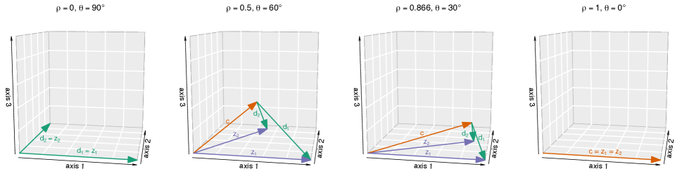
Figure 1: The D-CDLF decomposition for two standardized real random variables $z_{1}$ and $z_{2}$ with different values of their correlation $\rho$ and angle $\theta=\arccos\rho$.

Remark 1.

Since $z_{\operatorname{\mathfrak{I}}}$ only serves as an auxiliary role to form the three-dimensional space, we may write $c$ in an equivalent way as a complex random variable with $z_{\operatorname{\mathfrak{I}}}$ put on the imaginary part of $c$. That is, $c=(z_{1}+z_{2})\frac{\rho}{1+\rho}\pm\mathbf{i}z_{\operatorname{\mathfrak{I}}}\sqrt{\frac{\rho(1-\rho)}{1+\rho}}.$ Then the tri-orthogonality (5) holds in the space $\operatorname{span}_{\mathbb{R}}(\{z_{1},z_{2},\mathbf{i}z_{\operatorname{\mathfrak{I}}}\})$, where orthogonality is also equivalent to uncorrelatedness.

3.2 Decomposition of two real random vectors

We aim to extend the two-variable decomposition in previous subsection to any two real random vectors $\{\boldsymbol{x}_{k}\}_{k=1}^{2}$ in $(\mathcal{L}_{0}^{2},\operatorname{cov})$. Recall that the ACVs $(z_{k}^{(\ell)})_{\ell=1}^{r_{k}}=\boldsymbol{z}_{k}^{\top}$ of CCA given in Section 2.2 form an orthonormal basis of $\operatorname{span}(\boldsymbol{x}_{k}^{\top})$. We can thus write $\boldsymbol{x}_{k}$ as a linear combination of these ACVs and then apply the two-variable decomposition to each paired ACVs. Specifically, we have

$$\boldsymbol{x}_{k}=\sum_{\ell=1}^{r_{k}}\boldsymbol{\beta}_{k}^{(\ell)}z_{k}^{(\ell)}=\sum_{\ell=1}^{r_{k}}\boldsymbol{\beta}_{k}^{(\ell)}(c^{(\ell)}+d_{k}^{(\ell)})=\sum_{\ell=1}^{r_{c}}\boldsymbol{\beta}_{k}^{(\ell)}c^{(\ell)}+\sum_{\ell=1}^{r_{k}}\boldsymbol{\beta}_{k}^{(\ell)}d_{k}^{(\ell)},$$ (7)

where $z_{k}^{(\ell)}=c^{(\ell)}+d_{k}^{(\ell)}$, $c^{(\ell)}=c_{\operatorname{\mathfrak{R}}}^{(\ell)}+c_{\operatorname{\mathfrak{I}}}^{(\ell)}$ is given in (6) with $\{z_{1},z_{2},z_{\operatorname{\mathfrak{I}}},\rho\}$ replaced by $\{z_{1}^{(\ell)},z_{2}^{(\ell)},z_{\operatorname{\mathfrak{I}}}^{(\ell)},\rho^{(\ell)}\}$ for $\ell\leq r_{1}\wedge r_{2}$ and $c^{(\ell)}=0$ for $\ell>r_{1}\wedge r_{2}$, and $\mathbf{B}_{k}:=(\boldsymbol{\beta}_{k}^{(\ell)})_{\ell=1}^{r_{k}}=\operatorname{cov}(\boldsymbol{x}_{k},\boldsymbol{z}_{k})$. Note that $c^{(\ell)}=0$ for $r_{c}<\ell\leq r_{1}\wedge r_{2}$. For convenience, we set $\rho^{(\ell)}=0$ for $\ell>r_{1}\wedge r_{2}$.

From equation (7), we define $\{c^{(\ell)}\}_{\ell=1}^{r_{c}}$ as the CLFs of $\{\boldsymbol{x}_{k}\}_{k=1}^{2}$, and $\{d_{k}^{(\ell)}\}_{\ell=1}^{r_{k}}$ as the DLFs of $\boldsymbol{x}_{k}$. The common-source and distinctive-source random vectors, $\boldsymbol{c}_{k}$ and $\boldsymbol{d}_{k}$, of $\boldsymbol{x}_{k}$ are defined by

$$\boldsymbol{c}_{k} =\mathbf{B}_{k}^{[:,1:r_{c}]}[c^{(\ell)}]_{\ell=1}^{r_{c}}=\mathbf{B}_{k}^{[:,1:r_{c}]}[c_{\operatorname{\mathfrak{R}}}^{(\ell)}+c_{\operatorname{\mathfrak{I}}}^{(\ell)}]_{\ell=1}^{r_{c}}=:\boldsymbol{c}_{\operatorname{\mathfrak{R}},k}+\boldsymbol{c}_{\operatorname{\mathfrak{I}},k},$$ (8)

$$\boldsymbol{d}_{k} =\mathbf{B}_{k}[d_{k}^{(\ell)}]_{\ell=1}^{r_{k}}=\boldsymbol{x}_{k}-\boldsymbol{c}_{k}=(\boldsymbol{x}_{k}-\boldsymbol{c}_{\operatorname{\mathfrak{R}},k})-\boldsymbol{c}_{\operatorname{\mathfrak{I}},k}=:\boldsymbol{d}_{\operatorname{\mathfrak{R}},k}+\boldsymbol{d}_{\operatorname{\mathfrak{I}},k}.$$ (9)

Let $z_{\operatorname{\mathfrak{I}}}^{(\ell)}$ denote the auxiliary variable corresponding to $c^{(\ell)}$ in (6). We set $\{z_{\operatorname{\mathfrak{I}}}^{(\ell)}\}_{\ell=1}^{r_{c}}\perp\{z_{k}^{(\ell)}\}_{\ell\in[r_{k}],k\in[2]}$ and $z_{\operatorname{\mathfrak{I}}}^{(\ell_{1})}\perp z_{\operatorname{\mathfrak{I}}}^{(\ell_{2})}$ for $\ell_{1}\neq\ell_{2}$. Then by the bi-orthogonality of ACVs in (3), we obtain the orthogonality of CLFs and DLFs: $c^{(\ell_{1})}\perp c^{(\ell_{2})}$ and $d_{k}^{(\ell_{1})}\perp d_{k}^{(\ell_{2})}$ for $\ell_{1}\neq\ell_{2}$, $d_{1}^{(\ell_{1}^{\prime})}\perp d_{2}^{(\ell_{2}^{\prime})}$ for $\ell_{k}^{\prime}\in[r_{k}]$, and $\{c^{(\ell)}\}_{\ell=1}^{r_{c}}\perp\{d_{k}^{(\ell)}\}_{\ell\in[r_{k}],k\in[2]}$. In other words, we have the following desirable orthogonality:

$$\begin{cases}\operatorname{span}(\boldsymbol{c}_{1}^{\top})=\operatorname{span}(\boldsymbol{c}_{2}^{\top})=\operatorname{span}(\{c^{(\ell)}\}_{\ell=1}^{r_{c}}),\\ \operatorname{span}(\boldsymbol{d}_{1}^{\top})\perp\operatorname{span}(\boldsymbol{d}_{2}^{\top})~{}\text{with}~{}\operatorname{span}(\boldsymbol{d}_{k}^{\top})=\operatorname{span}(\{d_{k}^{(\ell)}\}_{\ell=1}^{r_{k}}),\\ \operatorname{span}(\boldsymbol{c}_{1}^{\top})\perp\operatorname{span}([\boldsymbol{d}_{1};\boldsymbol{d}_{2}]^{\top}).\end{cases}$$ (10)

From Proposition 1, the covariance matrices of $\boldsymbol{c}_{k}$ and $\boldsymbol{d}_{k}$ can be computed by

$$\operatorname{cov}(\boldsymbol{c}_{k}) =\mathbf{B}_{k}^{[:,1:r_{c}]}\operatorname{diag}([\rho^{(\ell)}]_{\ell=1}^{r_{c}})(\mathbf{B}_{k}^{[:,1:r_{c}]})^{\top},$$ (11)

$$\operatorname{cov}(\boldsymbol{d}_{k}) =\mathbf{B}_{k}\operatorname{diag}([1-\rho^{(\ell)}]_{\ell=1}^{r_{k}})\mathbf{B}_{k}^{\top}=\operatorname{cov}(\boldsymbol{x}_{k})-\operatorname{cov}(\boldsymbol{c}_{k}).$$ (12)

Theorem 1 (Uniqueness).

For $k\in\{1,2\}$, $\operatorname{cov}(\boldsymbol{c}_{k})$, $\operatorname{cov}(\boldsymbol{d}_{k})$, $\boldsymbol{c}_{\operatorname{\mathfrak{R}},k}$ and $\boldsymbol{d}_{\operatorname{\mathfrak{R}},k}$ given in (11), (12), (8) and (9) are unique to $\boldsymbol{x}_{k}$, regardless of the non-uniqueness of $\{z_{1}^{(\ell)}\}_{\ell=1}^{r_{1}}\cup\{z_{2}^{(\ell)}\}_{\ell=1}^{r_{2}}\cup\{z_{\operatorname{\mathfrak{I}}}^{(\ell)}\}_{\ell=1}^{r_{c}}$.

Remark 2.

Although the non-uniqueness of auxiliary variables $\{z_{\operatorname{\mathfrak{I}}}^{(\ell)}\}_{\ell=1}^{r_{c}}$ causes the non-identifiability issue of the CLF and DLF spaces $\{\operatorname{span}(\boldsymbol{c}_{k}^{\top}),\operatorname{span}(\boldsymbol{d}_{k}^{\top})\}_{k=1}^{2}$, the covariance of $\boldsymbol{x}_{k}$ explained by the CLFs and DLFs, i.e., $\operatorname{cov}(\boldsymbol{c}_{k})$ and $\operatorname{cov}(\boldsymbol{d}_{k})$, are invariant as shown in Theorem 1. Moreover, to build a predictive model for a real-valued outcome random vector $\boldsymbol{y}$ using $E(\boldsymbol{y}|\{c^{(\ell)}\}_{\ell=1}^{r_{c}},\{d_{k}^{(\ell)}\}_{\ell\in[r_{k}],k\in[2]},V,\{z_{\operatorname{\mathfrak{I}}}^{(\ell)}\}_{\ell=1}^{r_{c}})$, where $V$ is a set of real random variables (which can be empty), if we choose $[z_{\operatorname{\mathfrak{I}}}^{(\ell)}]_{\ell=1}^{r_{c}}$ to be independent of $[\boldsymbol{y};[c_{\operatorname{\mathfrak{R}}}^{(\ell)}]_{\ell=1}^{r_{c}};[[d_{\operatorname{\mathfrak{R}},k}^{(\ell)}]_{\ell\in[r_{k}]}]_{k\in[2]};[V]]$, then $E(\boldsymbol{y}|\{c^{(\ell)}\}_{\ell=1}^{r_{c}},\{d_{k}^{(\ell)}\}_{\ell\in[r_{k}],k\in[2]},V,\{z_{\operatorname{\mathfrak{I}}}^{(\ell)}\}_{\ell=1}^{r_{c}})=E(\boldsymbol{y}|\{c_{\operatorname{\mathfrak{R}}}^{(\ell)}\}_{\ell=1}^{r_{c}},\{d_{\operatorname{\mathfrak{R}},k}^{(\ell)}\}_{\ell\in[r_{k}],k\in[2]},V)$, and thus this predictive model is invariant to the non-uniqueness of $\{z_{\operatorname{\mathfrak{I}}}^{(\ell)}\}_{\ell=1}^{r_{c}}$.

Remark 3.

Our D-CDLF only differs from D-CCA (Shu et al., 2020) in the CLFs $\{c^{(\ell)}\}_{\ell=1}^{r_{c}}$. D-CCA defines its $\ell$-th CLF as $c^{(\ell)}=(z_{1}^{(\ell)}+z_{2}^{(\ell)})/\big{(}2-2\sqrt{(1-\rho^{(\ell)})/(1+\rho^{(\ell)})}\big{)}$, which satisfies $\big{(}1+\sqrt{1-(\rho^{(\ell)})^{2}}\big{)}\operatorname{var}(c^{(\ell)})=(\rho^{(\ell)})^{2}\leq\rho^{(\ell)}$. Since D-CDLF has $\operatorname{var}(c^{(\ell)})=\rho^{(\ell)}$ and both methods have $\operatorname{var}(\boldsymbol{c}_{k}^{[i]})=\sum_{\ell=1}^{r_{c}}(\mathbf{B}_{k}^{[i,\ell]})^{2}\operatorname{var}(c^{(\ell)})$, it concludes that the variance $\operatorname{var}(\boldsymbol{c}_{k}^{[i]})$ of D-CCA is no larger than that of D-CDLF.

3.3 Variable-level and view-level PVEs

To measure the joint effect of CLFs or DLFs on original variables, we propose the variable-level PVEs and the view-level PVEs.

The variable-level PVEs for a denoised original variable $\boldsymbol{x}_{k}^{[i]}$ by CLFs $\{c^{(\ell)}\}_{\ell=1}^{r_{c}}$ and its DLFs $\{d_{k}^{(\ell)}\}_{\ell=1}^{r_{k}}$ are, respectively, defined as

$$\operatorname{PVE}_{c}(\boldsymbol{x}_{k}^{[i]}):=\frac{\operatorname{var}(\boldsymbol{c}_{k}^{[i]})}{\operatorname{var}(\boldsymbol{x}_{k}^{[i]})}=\sum_{\ell=1}^{r_{c}}\operatorname{corr}^{2}(\boldsymbol{x}_{k}^{[i]},c^{(\ell)}),$$

and

$$\operatorname{PVE}_{d}(\boldsymbol{x}_{k}^{[i]}):=\frac{\operatorname{var}(\boldsymbol{d}_{k}^{[i]})}{\operatorname{var}(\boldsymbol{x}_{k}^{[i]})}=\sum_{\ell=1}^{r_{k}}\operatorname{corr}^{2}(\boldsymbol{x}_{k}^{[i]},d_{k}^{(\ell)}),$$

which are equal to the sums of their squared correlations. The variable-level PVEs are useful in selecting original variables within each data view that are highly affected by CLFs and DLFs, respectively.

The view-level PVEs for the entire $\boldsymbol{x}_{k}$ by CLFs $\{c^{(\ell)}\}_{\ell=1}^{r_{c}}$ and its DLFs $\{d_{k}^{(\ell)}\}_{\ell=1}^{r_{k}}$ are, respectively, defined as

$$\operatorname{PVE}_{c}(\boldsymbol{x}_{k}):=\frac{\sum_{i=1}^{p_{k}}\operatorname{var}(\boldsymbol{c}_{k}^{[i]})}{\sum_{i=1}^{p_{k}}\operatorname{var}(\boldsymbol{x}_{k}^{[i]})}=\sum_{i=1}^{p_{k}}\gamma_{ki}\operatorname{PVE}_{c}(\boldsymbol{x}_{k}^{[i]})$$

and

$$\operatorname{PVE}_{d}(\boldsymbol{x}_{k}):=\frac{\sum_{i=1}^{p_{k}}\operatorname{var}(\boldsymbol{d}_{k}^{[i]})}{\sum_{i=1}^{p_{k}}\operatorname{var}(\boldsymbol{x}_{k}^{[i]})}=\sum_{i=1}^{p_{k}}\gamma_{ki}\operatorname{PVE}_{d}(\boldsymbol{x}_{k}^{[i]}),$$

which are the weighted averages of corresponding variable-level PVEs with weights $\gamma_{ki}=\operatorname{var}(\boldsymbol{x}_{k}^{[i]})/\sum_{j=1}^{p_{k}}\operatorname{var}(\boldsymbol{x}_{k}^{[j]})$.

Due to the uncorrelatedness between CLFs and DLFs, the two types of PVEs follow the rule of sum:

$$\operatorname{PVE}_{c}(\boldsymbol{x}_{k}^{[i]})+\operatorname{PVE}_{d}(\boldsymbol{x}_{k}^{[i]})=1\qquad\text{and}\qquad\operatorname{PVE}_{c}(\boldsymbol{x}_{k})+\operatorname{PVE}_{d}(\boldsymbol{x}_{k})=1.$$

4 Estimation

Suppose that the high-dimensional low-rank plus noise structure in (1) follows the factor model (Shu et al., 2022):

$$\mathbf{Y}_{k}=\mathbf{X}_{k}+\mathbf{E}_{k}=\mathbf{B}_{k,f}\mathbf{F}_{k}+\mathbf{E}_{k},\qquad\boldsymbol{y}_{k}=\boldsymbol{x}_{k}+\boldsymbol{e}_{k}=\mathbf{B}_{k,f}\boldsymbol{f}_{k}+\boldsymbol{e}_{k},\qquad k=1,2,$$ (13)

where $\mathbf{B}_{k,f}\in\mathbb{R}^{p_{k}\times r_{k}}$ is a deterministic matrix, the columns of $\mathbf{Y}_{k}$, $\mathbf{X}_{k}$, $\mathbf{F}_{k}$ and $\mathbf{E}_{k}$ are the $n$ i.i.d. copies of $\boldsymbol{y}_{k}$, $\boldsymbol{x}_{k}$, $\boldsymbol{f}_{k}$ and $\boldsymbol{e}_{k}$, respectively, $\boldsymbol{f}_{k}^{\top}$ is an orthonormal basis of $\operatorname{span}(\boldsymbol{x}_{k}^{\top})$ with $\operatorname{cov}(\boldsymbol{f}_{k},\boldsymbol{e}_{k})=\mathbf{0}_{r_{k}\times p_{k}}$, $\operatorname{span}(\boldsymbol{x}_{k}^{\top})$ is a fixed space that is independent of $\{p_{k}\}_{k=1}^{2}$ and $n$, and $\mathbf{F}:=[\mathbf{F}_{1};\mathbf{F}_{2}]$ has independent columns. We assume that $\operatorname{cov}(\boldsymbol{y}_{k})$ is a spiked covariance matrix, for which the largest $r_{k}$ eigenvalues are significantly larger than the rest, i.e., signals are distinguishably stronger than noises. The $r_{k}$ spiked eigenvalues are majorly contributed by signal $\boldsymbol{x}_{k}$, whereas the rest small eigenvalues are induced by noise $\boldsymbol{e}_{k}$. The spiked covariance model has been widely used in various fields, such as signal processing (Nadakuditi and Silverstein, 2010), machine learning (Huang, 2017), and economics (Chamberlain and Rothschild, 1983).

For simplicity, we define D-CDLF estimators using true $\{r_{k}\}_{k=1}^{2}$ and $r_{c}$, which can be estimated by the edge distribution (ED) method of Onatski (2010) and the minimum description length information-theoretic criterion (MDL-IC) of Song et al. (2016), respectively. See Section 2.3 in Shu et al. (2020) for details.

The estimator of $\mathbf{X}_{k}$ is defined by using the soft-thresholding method of Shu et al. (2020) as

$$\widehat{\mathbf{X}}_{k}=\mathbf{U}_{k1}\operatorname{diag}([\widehat{\sigma}_{\ell}^{S}(\mathbf{Y}_{k})]_{\ell=1}^{r_{k}})\mathbf{U}_{k2}^{\top},$$ (14)

where $\mathbf{U}_{k1}\operatorname{diag}([\sigma_{\ell}(\mathbf{Y}_{k})]_{\ell=1}^{r_{k}})\mathbf{U}_{k2}^{\top}$ is the top-$r_{k}$ SVD of $\mathbf{Y}_{k}$, and the soft-thresholded singular value $\widehat{\sigma}_{\ell}^{S}(\mathbf{Y}_{k})=\sqrt{\max\{\sigma_{\ell}^{2}(\mathbf{Y}_{k})-\tau_{k}p_{k},0\}}$ with $\tau_{k}=\sum_{\ell=r_{k}+1}^{p_{k}}\sigma_{\ell}^{2}(\mathbf{Y}_{k})/(np_{k}-nr_{k}-p_{k}r_{k}).$ Define the estimator of $\mathbf{\operatorname{cov}}(\boldsymbol{x}_{k})$ by

$$\widehat{\mathbf{\operatorname{cov}}}(\boldsymbol{x}_{k})=n^{-1}\widehat{\mathbf{X}}_{k}\widehat{\mathbf{X}}_{k}^{\top},$$ (15)

and denote its top-$r_{k}$ SVD by $\widehat{\mathbf{\Sigma}}_{k}=\widehat{\mathbf{V}}_{k}\widehat{\mathbf{\Lambda}}_{k}\widehat{\mathbf{V}}_{k}^{\top}$, where $\widehat{\mathbf{\Lambda}}_{k}=\operatorname{diag}([\sigma_{\ell}(\widehat{\operatorname{cov}}(\boldsymbol{x}_{k})]_{\ell=1}^{r_{k}})$. Let $\widehat{\mathbf{H}}_{k}=(\widehat{\mathbf{\Lambda}}_{k}^{\dagger})^{1/2}\widehat{\mathbf{V}}_{k}^{\top}\widehat{\mathbf{X}}_{k}$, which is the estimated sample matrix of $\boldsymbol{h}_{k}=\mathbf{\Lambda}_{k}^{-1/2}\mathbf{V}_{k}^{\top}\boldsymbol{x}_{k}$. Define the estimator of $\mathbf{\Theta}=\operatorname{cov}(\boldsymbol{h}_{1},\boldsymbol{h}_{2})$ by $\widehat{\mathbf{\Theta}}=n^{-1}\widehat{\mathbf{H}}_{1}\widehat{\mathbf{H}}_{2}^{\top}$. Write the full SVD of $\widehat{\mathbf{\Theta}}$ by $\widehat{\mathbf{\Theta}}=\widehat{\mathbf{U}}_{\theta,1}\widehat{\mathbf{\Lambda}}_{\theta}\widehat{\mathbf{U}}_{\theta,2}^{\top}$. The sample matrix of $\boldsymbol{z}_{k}$, the vector consisting of $\boldsymbol{x}_{k}$’s ACVs, is estimated by $\widehat{\mathbf{Z}}_{k}=\widehat{\mathbf{U}}_{\theta,k}^{\top}\widehat{\mathbf{H}}_{k}$. We define the estimators of the canonical correlation $\rho^{(\ell)}=\sigma_{\ell}(\mathbf{\Theta})$ and the coefficient matrix $\mathbf{B}_{k}=\operatorname{cov}(\boldsymbol{x}_{k},\boldsymbol{z}_{k})=\mathbf{V}_{k}\mathbf{\Lambda}_{k}^{1/2}\mathbf{U}_{\theta,k}$, respectively, by

$$\widehat{\rho}^{(\ell)}=\sigma_{\ell}(\widehat{\mathbf{\Theta}})\quad\text{and}\quad\widehat{\mathbf{B}}_{k}=n^{-1}\widehat{\mathbf{X}}_{k}\widehat{\mathbf{Z}}_{k}^{\top}=\widehat{\mathbf{V}}_{k}\widehat{\mathbf{\Lambda}}_{k}^{1/2}\widehat{\mathbf{U}}_{\theta,k}.$$ (16)

Then from the expressions of $\operatorname{cov}(\boldsymbol{c}_{k})$ and $\operatorname{cov}(\boldsymbol{d}_{k})$ given in (11) and (12), their estimators are defined as

$$\widehat{\operatorname{cov}}(\boldsymbol{c}_{k}) =\widehat{\mathbf{B}}_{k}^{[:,1:r_{c}]}\operatorname{diag}([\widehat{\rho}_{\ell}]_{\ell=1}^{r_{c}})(\widehat{\mathbf{B}}_{k}^{[:,1:r_{c}]})^{\top},$$ (17)

$$\widehat{\operatorname{cov}}(\boldsymbol{d}_{k}) =\widehat{\operatorname{cov}}(\boldsymbol{x}_{k})-\widehat{\operatorname{cov}}(\boldsymbol{c}_{k}).$$ (18)

The proportions of signal variance explained by CLFs and DLFs are estimated by

$$\widehat{\operatorname{PVE}}_{c}(\boldsymbol{x}_{k}) =\frac{\operatorname{tr}(\widehat{\operatorname{cov}}(\boldsymbol{c}_{k}))}{\operatorname{tr}(\widehat{\operatorname{cov}}(\boldsymbol{x}_{k}))}=1-\frac{\operatorname{tr}(\widehat{\operatorname{cov}}(\boldsymbol{d}_{k}))}{\operatorname{tr}(\widehat{\operatorname{cov}}(\boldsymbol{x}_{k}))}=1-\widehat{\operatorname{PVE}}_{d}(\boldsymbol{x}_{k}),$$

$$\widehat{\operatorname{PVE}}_{c}(\boldsymbol{x}_{k}^{[i]}) =\frac{\widehat{\operatorname{var}}(\boldsymbol{c}_{k}^{[i]})}{\widehat{\operatorname{var}}(\boldsymbol{x}_{k}^{[i]})}=1-\frac{\widehat{\operatorname{var}}(\boldsymbol{d}_{k}^{[i]})}{\widehat{\operatorname{var}}(\boldsymbol{x}_{k}^{[i]})}=1-\widehat{\operatorname{PVE}}_{d}(\boldsymbol{x}_{k}^{[i]}),$$

where $\widehat{\operatorname{var}}(\boldsymbol{v}_{k}^{[i]})=\widehat{\operatorname{cov}}(\boldsymbol{v}_{k})^{[i,i]}$ for $\boldsymbol{v}_{k}\in\{\boldsymbol{x}_{k},\boldsymbol{c}_{k},\boldsymbol{d}_{k}\}$.

To estimate the common-source and distinctive-source matrices $\{\mathbf{C}_{k},\mathbf{D}_{k}\}$, i.e., the sample matrices of $\{\boldsymbol{c}_{k},\boldsymbol{d}_{k}\}$, we first need to find a centered isotropic random vector $\boldsymbol{z}_{\operatorname{\mathfrak{I}}}=[z_{\operatorname{\mathfrak{I}}}^{(\ell)}]_{\ell=1}^{r_{c}}$ such that $\operatorname{span}(\boldsymbol{z}_{\operatorname{\mathfrak{I}}}^{\top})\perp\operatorname{span}([\boldsymbol{x}_{k}]_{k\in[K]}^{\top})$, and its sample matrix $\mathbf{Z}_{\operatorname{\mathfrak{I}}}$. We generate $\{z_{\operatorname{\mathfrak{I}}}^{(\ell)}\}_{\ell=1}^{r_{c}}$ as i.i.d. standard Gaussian random variables independent of $\{\boldsymbol{x}_{k}\}_{k=1}^{2}$ by using a Gaussian random number generator. Following the definitions of $\{\boldsymbol{c}_{k},\boldsymbol{d}_{k}\}$ in (8) and (9), we define the estimators of their sample matrices corresponding to $\{\mathbf{X}_{1},\mathbf{X}_{2}\}$ by

$$\widehat{\mathbf{C}}_{k}=\widehat{\mathbf{B}}_{k}^{[:,1:r_{c}]}[\widehat{\boldsymbol{c}}^{(\ell)}]_{\ell=1}^{r_{c}}\quad\text{and}\quad\widehat{\mathbf{D}}_{k}=\widehat{\mathbf{B}}_{k}[\widehat{\boldsymbol{d}}_{k}^{(\ell)}]_{\ell=1}^{r_{k}}=\widehat{\mathbf{X}}_{k}-\widehat{\mathbf{C}}_{k},$$ (19)

where $\widehat{\boldsymbol{c}}^{(\ell)}$, $\widehat{\boldsymbol{d}}_{k}^{(\ell)}\in\mathbb{R}^{1\times n}$ are estimated samples of $c^{(\ell)}$ and $d_{k}^{(\ell)}$ defined by

$$\widehat{\boldsymbol{c}}^{(\ell)}=\frac{\widehat{\rho}^{(\ell)}}{1+\widehat{\rho}^{(\ell)}}(\widehat{\mathbf{Z}}_{1}^{[\ell,:]}+\widehat{\mathbf{Z}}_{2}^{[\ell,:]})+\mathbf{Z}_{\operatorname{\mathfrak{I}}}^{[\ell,:]}\sqrt{\frac{\widehat{\rho}^{(\ell)}(1-\widehat{\rho}^{(\ell)})}{1+\widehat{\rho}^{(\ell)}}}\quad\text{and}\quad\widehat{\boldsymbol{d}}_{k}^{(\ell)}=\widehat{\mathbf{Z}}_{k}^{[\ell,:]}-\widehat{\boldsymbol{c}}^{(\ell)}$$ (20)

for $\ell\leq r_{c}$, and $\widehat{\boldsymbol{d}}_{k}^{(\ell)}=\widehat{\mathbf{Z}}_{k}^{[\ell,:]}$ for $\ell>r_{c}$ due to $\rho^{(\ell)}=0$, and $\widehat{\mathbf{Z}}_{k}$ and $\{\widehat{\rho}^{(\ell)},\widehat{\mathbf{B}}_{k}\}$ are given above and in (16), respectively.

5 Theoretical Proofs

Proof of Proposition 1.

Let $z_{\operatorname{\mathfrak{I}}}\perp\{z_{1},z_{2}\}$, and $w=a_{1}z_{1}+a_{2}z_{2}+a_{\operatorname{\mathfrak{I}}}z_{\operatorname{\mathfrak{I}}}$ with $\operatorname{var}(w)=a_{1}^{2}+a_{2}^{2}+2a_{1}a_{2}\rho+a_{\operatorname{\mathfrak{I}}}^{2}=1$. Let $c=\alpha w$. We have

$$\operatorname{cov}(c,d_{1})=\operatorname{cov}(c,z_{1}-c) =\operatorname{cov}(c,z_{1})-\alpha^{2}$$

$$=\alpha(a_{1}+a_{2}\rho)-\alpha^{2}=0$$ (21)

and

$$\operatorname{cov}(c,d_{2})=\operatorname{cov}(c,z_{2}-c) =\operatorname{cov}(c,z_{2})-\alpha^{2}$$

$$=\alpha(a_{2}+a_{1}\rho)-\alpha^{2}=0.$$ (22)

So, $\sum_{k=1}^{2}\operatorname{cov}(z_{k},c)=2\alpha^{2}$. Consequently,

$$\operatorname{cov}(d_{1},d_{2})=\operatorname{cov}(z_{1}-c,z_{2}-c)=\operatorname{cov}(z_{1},z_{2})-\sum_{k=1}^{2}\operatorname{cov}(z_{k},c)+\alpha^{2}=\rho-\alpha^{2}=0$$

yields

$$\alpha=\pm\sqrt{\rho}.$$ (23)

Also from (21) and (22), we obtain

$$\alpha(1+\rho)(a_{1}+a_{2})=2\alpha^{2},$$ (24)

$$\alpha(a_{1}+a_{2}\rho)=\alpha^{2},$$ (25)

and

$$\alpha(a_{2}+a_{1}\rho)=\alpha^{2}.$$ (26)

When $\rho=0$, then by (23) we have $\alpha=0$ and thus $c=\alpha w=0$.

We next consider $\rho\in(0,1]$. Then from equations (23)–(26), we have

$$a_{1}+a_{2}=2\alpha/(1+\rho)$$ (27)

and

$$a_{1}+a_{2}\rho=a_{2}+a_{1}\rho=\alpha.$$

Hence, $1-a_{\operatorname{\mathfrak{I}}}^{2}=a_{1}^{2}+2a_{1}a_{2}\rho+a_{2}^{2}=\alpha(a_{1}+a_{2})=2\rho/(1+\rho)$. So,

$$a_{\operatorname{\mathfrak{I}}}=\pm\sqrt{\frac{1-\rho}{1+\rho}}\ \text{for}\ \rho\in(0,1].$$ (28)

Moreover, $(a_{1}+a_{2})^{2}=4\rho/(1+\rho)^{2}=1-2a_{1}a_{2}\rho-a_{\operatorname{\mathfrak{I}}}^{2}+2a_{1}a_{2}$, and thus $2a_{1}a_{2}(1-\rho)=4\rho/(1+\rho)^{2}-1+a_{\operatorname{\mathfrak{I}}}^{2}=4\rho/(1+\rho)^{2}-2\rho/(1+\rho)=2\rho(1-\rho)/(1+\rho)^{2}$. Further let $\rho\in(0,1)$, then $a_{1}a_{2}=\rho/(1+\rho)^{2}$. Consequently, $(a_{1}-a_{2})^{2}=(a_{1}+a_{2})^{2}-4a_{1}a_{2}=4\rho/(1+\rho)^{2}-4\rho/(1+\rho)^{2}=0$. Then from (27), $a_{1}=a_{2}=\alpha/(1+\rho).$ We hence obtain

$$c=\alpha w=\alpha(a_{1}z_{1}+a_{2}z_{2}+a_{\operatorname{\mathfrak{I}}}z_{\operatorname{\mathfrak{I}}})=\frac{\rho}{1+\rho}(z_{1}+z_{2})\pm z_{\operatorname{\mathfrak{I}}}\sqrt{\frac{\rho(1-\rho)}{1+\rho}}$$ (29)

for $\rho\in(0,1)$.

When $\rho=1$, we have $z_{1}=z_{2}$, and moreover, by (28) we have $a_{\operatorname{\mathfrak{I}}}=0$. Then by (27) and (23), $c=\alpha w=\alpha(a_{1}z_{1}+a_{2}z_{2}+a_{\operatorname{\mathfrak{I}}}z_{\operatorname{\mathfrak{I}}})=\alpha(a_{1}+a_{2})z_{1}=2\alpha^{2}z_{1}/(1+\rho)=2\rho z_{1}/(1+\rho)=(z_{1}+z_{2})\rho/(1+\rho)$. The equation $c=(z_{1}+z_{2})\rho/(1+\rho)$ satisfies (29) for $\rho=1$.

From the above, for $\rho\in[0,1]$ we have

$$c=\frac{\rho}{1+\rho}(z_{1}+z_{2})\pm z_{\operatorname{\mathfrak{I}}}\sqrt{\frac{\rho(1-\rho)}{1+\rho}}$$

and $\operatorname{var}(c)=\alpha^{2}=\rho$. By $c\perp d_{k}$ for $k=1,2$, we have $\operatorname{var}(d_{k})=\operatorname{var}(z_{k})-\operatorname{var}(c)=1-\rho$. ∎

Proof of Theorem 1.

Let $\{\widetilde{\boldsymbol{z}}_{k}^{[1:r_{c}]}\}_{k=1}^{2}$ be an arbitrary set of the first $r_{c}$ pairs of canonical variables of $\{\boldsymbol{x}_{k}\}_{k=1}^{2}$. From the proof of Theorem 2 in Shu et al. (2020), we have that there exists a matrix $\mathbf{Q}_{\theta}=\operatorname{diag}(\{\mathbf{Q}_{\theta\ell}\}_{\ell=1}^{r_{c}^{*}})$ such that $\widetilde{\boldsymbol{z}}_{k}^{[1:r_{c}]}=\mathbf{Q}_{\theta}\boldsymbol{z}_{k}^{[1:r_{c}]}$, where $\mathbf{Q}_{\theta\ell}$ is an orthogonal matrix with column dimension equal to the repetition number of the $\ell$-th largest distinct value in $\rho_{1},\dots,\rho_{r_{c}}$. Then,

$$\operatorname{cov}(\boldsymbol{x}_{k},\widetilde{\boldsymbol{z}}_{k}^{[1:r_{c}]})\operatorname{diag}(\rho_{1},\dots,\rho_{r_{c}})\operatorname{cov}(\widetilde{\boldsymbol{z}}_{k}^{[1:r_{c}]},\boldsymbol{x}_{k})$$ (30)

$$=\operatorname{cov}(\boldsymbol{x}_{k},\boldsymbol{z}_{k}^{[1:r_{c}]})\mathbf{Q}_{\theta}^{\top}\operatorname{diag}(\rho_{1},\dots,\rho_{r_{c}})\mathbf{Q}_{\theta}\operatorname{cov}(\boldsymbol{z}_{k}^{[1:r_{c}]},\boldsymbol{x}_{k})$$

$$=\operatorname{cov}(\boldsymbol{x}_{k},\boldsymbol{z}_{k}^{[1:r_{c}]})\operatorname{diag}(\rho_{1},\dots,\rho_{r_{c}})\operatorname{cov}(\boldsymbol{z}_{k}^{[1:r_{c}]},\boldsymbol{x}_{k})$$ (31)

$$=\operatorname{cov}(\boldsymbol{x}_{k},\boldsymbol{z}_{k}^{[1:r_{c}]})\operatorname{cov}((c_{1},\dots,c_{r_{c}})^{\top})\operatorname{cov}(\boldsymbol{z}_{k}^{[1:r_{c}]},\boldsymbol{x}_{k})$$

$$=\operatorname{cov}(\operatorname{cov}(\boldsymbol{x}_{k},\boldsymbol{z}_{k}^{[1:r_{c}]})(c_{1},\dots,c_{r_{c}})^{\top})$$

$$=\operatorname{cov}(\boldsymbol{c}_{k}).$$

By (30) and (31), $\operatorname{cov}(\boldsymbol{c}_{k})=\operatorname{cov}(\boldsymbol{x}_{k},\boldsymbol{z}_{k}^{[1:r_{c}]})\operatorname{diag}(\rho_{1},\dots,\rho_{r_{c}})\operatorname{cov}(\boldsymbol{z}_{k}^{[1:r_{c}]},\boldsymbol{x}_{k})$ is unique.

Since $\operatorname{span}(\boldsymbol{c}_{k}^{\top})\perp\operatorname{span}(\boldsymbol{d}_{k}^{\top})$, that is, $\operatorname{cov}(\boldsymbol{c}_{k},\boldsymbol{d}_{k})=\mathbf{0}_{p_{k}\times p_{k}}$, we have that $\operatorname{cov}(\boldsymbol{x}_{k})=\operatorname{cov}(\boldsymbol{c}_{k}+\boldsymbol{d}_{k})=\operatorname{cov}(\boldsymbol{c}_{k})+\operatorname{cov}(\boldsymbol{d}_{k})$. Thus, $\operatorname{cov}(\boldsymbol{d}_{k})=\operatorname{cov}(\boldsymbol{x}_{k})-\operatorname{cov}(\boldsymbol{c}_{k})$ is also unique, and $\operatorname{cov}(\boldsymbol{d}_{k})=\mathbf{B}_{k}\mathbf{B}_{k}^{\top}-\mathbf{B}_{k}\operatorname{diag}([\rho_{\ell}]_{\ell=1}^{r_{k}})\mathbf{B}_{k}^{\top}=\mathbf{B}_{k}\operatorname{diag}([1-\rho_{\ell}]_{\ell=1}^{r_{k}})\mathbf{B}_{k}^{\top}$.

Following the same proof technique used for Theorem 2 in Shu et al. (2020), we obtain the uniqueness of $\boldsymbol{c}_{\operatorname{\mathfrak{R}},k}$ and $\boldsymbol{d}_{\operatorname{\mathfrak{R}},k}$. ∎

References

• Chamberlain and Rothschild (1983) Chamberlain, G. and Rothschild, M. (1983), “Arbitrage, factor structure, and mean-variance analysis on large asset markets,” Econometrica, 51, 1281–1304.
• Feng et al. (2018) Feng, Q., Jiang, M., Hannig, J., and Marron, J. (2018), “Angle-based joint and individual variation explained,” Journal of Multivariate Analysis, 166, 241–265.
• Gaynanova and Li (2019) Gaynanova, I. and Li, G. (2019), “Structural learning and integrative decomposition of multi-view data,” Biometrics, 75, 1121–1132.
• Hotelling (1936) Hotelling, H. (1936), “Relations between two sets of variates,” Biometrika, 28, 321–377.
• Huang (2017) Huang, H. (2017), “Asymptotic behavior of support vector machine for spiked population model,” Journal of Machine Learning Research, 18, 1–21.
• Lock et al. (2013) Lock, E. F., Hoadley, K. A., Marron, J. S., and Nobel, A. B. (2013), “Joint and individual variation explained (JIVE) for integrated analysis of multiple data types,” Annals of Applied Statistics, 7, 523–542.
• Löfstedt and Trygg (2011) Löfstedt, T. and Trygg, J. (2011), “OnPLS–a novel multiblock method for the modelling of predictive and orthogonal variation,” Journal of Chemometrics, 25, 441–455.
• Nadakuditi and Silverstein (2010) Nadakuditi, R. R. and Silverstein, J. W. (2010), “Fundamental limit of sample generalized eigenvalue based detection of signals in noise using relatively few signal-bearing and noise-only samples,” IEEE Journal of Selected Topics in Signal Processing, 4, 468–480.
• O’Connell and Lock (2016) O’Connell, M. J. and Lock, E. F. (2016), “R.JIVE for exploration of multi-source molecular data,” Bioinformatics, 32, 2877–2879.
• Onatski (2010) Onatski, A. (2010), “Determining the number of factors from empirical distribution of eigenvalues,” The Review of Economics and Statistics, 92, 1004–1016.
• Schouteden et al. (2013) Schouteden, M., Van Deun, K., Pattyn, S., and Van Mechelen, I. (2013), “SCA with rotation to distinguish common and distinctive information in linked data,” Behavior research methods, 45, 822–833.
• Shiryaev (1996) Shiryaev, A. N. (1996), Probability, vol. 95 of Graduate Texts in Mathematics, Springer-Verlag, New York, 2nd ed., translated from the first (1980) Russian edition by R. P. Boas.
• Shu et al. (2022) Shu, H., Qu, Z., and Zhu, H. (2022), “D-GCCA: Decomposition-based Generalized Canonical Correlation Analysis for Multi-view High-dimensional Data,” Journal of Machine Learning Research, 23, 1–64.
• Shu et al. (2020) Shu, H., Wang, X., and Zhu, H. (2020), “D-CCA: A decomposition-based canonical correlation analysis for high-dimensional datasets,” Journal of the American Statistical Association, 115, 292–306.
• Song et al. (2016) Song, Y., Schreier, P. J., Ramírez, D., and Hasija, T. (2016), “Canonical correlation analysis of high-dimensional data with very small sample support,” Signal Processing, 128, 449–458.
• Yin et al. (1988) Yin, Y.-Q., Bai, Z.-D., and Krishnaiah, P. R. (1988), “On the limit of the largest eigenvalue of the large dimensional sample covariance matrix,” Probability Theory and Related Fields, 78, 509–521.
• Zhou et al. (2016) Zhou, G., Cichocki, A., Zhang, Y., and Mandic, D. P. (2016), “Group component analysis for multiblock data: Common and individual feature extraction,” IEEE Transactions on Neural Networks and Learning Systems, 27, 2426–2439.