On restrictions of current warp drive spacetimes
and immediate possibilities of improvement

Abstract

Looking at current proposals of so-called ‘warp drive spacetimes’, they appear to employ General Relativity only at an elementary level. A number of strong restrictions are imposed such as flow-orthogonality of the spacetime foliation, vanishing spatial Ricci tensor, dimensionally reduced and coordinate-dependent velocity fields, to mention the main restrictions. We here provide a brief summary of our proposal of a general and covariant description of spatial motions within General Relativity, then discuss the restrictions that are employed in the majority of the current literature. That current warp drive models are discussed to be unphysical may not be surprising; they lack important ingredients such as covariantly non-vanishing spatial velocity, acceleration, vorticity, together with curved space, and a warp mechanism.

1 Brief recap on the state-of-the-art of warp drive spacetimes

The description of accelerated motions within Special Relativity (SR) enjoys popularity in lectures and exercises when applied to the idea of space travel (see, e.g., [16, 22, 24]). However, such travels described within SR face limitations due to the flatness of spacetime and lightcone barrier (see, e.g., [14] for stimulating thoughts and discussions).

A smarter way to think of space travels was put forward by Alcubierre [2] (see also [4]), motivated by notions of science fiction. Alcubierre aimed at exploiting the far-reaching possibilities offered by General Relativity (GR). Since expansion or contraction of space does not fall under the special-relativistic limitation of the speed of light—although locally causality is respected—a hyperfast space travel seems to be possible by actively deforming the gravitational field that, according to Einstein, defines the spacetime geometry. Often, the recession velocity in a globally expanding cosmological model is employed as an example where the speed of light can be exceeded, while an (comoving) observer in the Universe would be confined to the Hubble sphere (cf., e.g., [12, 11]).

Since Alcubierre’s proposal, a substantial body of literature has been developed that is essentially based on the space travel design introduced by Alcubierre and later Natário who dropped the restriction of a one-component coordinate velocity field (related to the shift vector field) and considered the possibility of vanishing expansion [23]. The subject of spacetime engineering also caught the attention of researchers at space agencies, realizing the potential of such theoretical ideas, e.g., [29, 30] and [18, 19]. In [26], the authors summarize most of the literature assigning the wording ‘generic warp drives’ to these concepts. We refer to this paper for a comprehensive list of references, but we do not comment on its contents here. Contrary to the wording ‘generic’ we here name those concepts ‘restricted warp drives’ (R-Warp for short), and we shall explain how we can and should drop a number of highly restricting assumptions.

This Letter concentrates on the covariant description of spatial motion in GR as opposed to the coordinate-dependent architecture of current warp drive proposals. We think that such a description is key to open the possibility of a future definition of what the idea behind warp drive means in terms of Einstein’s equations. We shall remain within classical GR and also leave the description of extended ‘warp bubbles’ and their motion to later works. We emphasize that current proposals are confined to describe motions within a given 3+1 foliation of spacetime, hence are subject to the classical Cauchy problem of GR. The idea of warp drive implies an active gravity control or spacetime engineering process that locally changes the spacetime structure during the travel. We think that there is a long way ahead to arrive at a physical definition of warp drive. In particular, we notice that current proposals do not introduce a warp mechanism, mainly due to an externally given velocity. Said this, we employ the wording ‘warp’ to exhibit the aim of our path towards this concept. A next step consists in establishing all evolution equations, constraints and conservation laws governing the warp field, linking all relevant fields to variables that could eventually be actively controlled by the spaceship.

We organize this Letter as follows. In Section 2.1 we shall first recall well-known geometrical concepts for the description of covariant spatial motions and their kinematics. We then put currently employed restrictions into perspective and explore properties of R-Warp designs in Section 2.2. We contrast this restricted concept to our proposal of tilted warp drives (T-Warp for short) within the covariant setting in Section 2.3, followed by a comparison of the two concepts in Section 2.4. In Section 3 we lay down a strategy on how to improve on current warp drive realizations and discuss some perspectives. This Letter is chiefly based on and inspired by formalism developed in the context of inhomogeneous cosmology [10].

Notations: Throughout this Letter, bold letters are used for coordinate-free notation of given vector and tensor fields whose components are given in local coordinate bases $\{\bm{{\mathrm{d}}}x^{\alpha},\bm{\partial}_{\alpha}\}$ with $\left(x^{\mu}\right)=\left(t,x^{i}\right)\equiv\left(t,\bm{x}\right)$, where Greek indices denote the spacetime coordinates on $(\mathcal{M},\bf g)$, the spacetime manifold equipped with a Lorentzian metric, whereas Latin indices stand for spatial coordinates. We set the speed of light $c=1$.

2 Covariant spatial motion

2.1 General kinematics of covariant spatial motion

The current literature on warp drive spacetimes is based on a 3+1 decomposition of spacetime, foliated into spatial leaves $\Sigma_{t}$ with the unit normal $\bm{n}$, i.e., $\mathcal{M}=I\times\Sigma_{t}$ with $t\in I\subset\mathbb{R}$. The components of $\bm{n}$ and its metric dual $1$-form, are given by

$$\bm{n}=\frac{1}{N}\left(1,-\bm{N}\right)\,,\quad{\bm{n}}^{\flat}=-N\,(1,\bm{0})\,,$$ (2.1)

where $N$ is the lapse function and $\bm{N}=N^{i}\bm{\partial}_{i}$ is the shift vector (cf., e.g., [10, 27, 15]).

The bilinear form $\mathbf{h}=h_{\alpha\beta}\,\mathbf{d}x^{\alpha}\otimes\mathbf{d}x^{\beta}$ on $\Sigma_{t}$ can be used to project spacetime tensors onto the hypersurfaces of the foliation and has the following form and properties:

$$h_{\mu\nu}:=g_{\mu\nu}+n_{\mu}n_{\nu}\,,\quad h_{\alpha\mu}n^{\alpha}=0\,,\quad\tensor{h}{{}^{\mu}_{\alpha}}\tensor{h}{{}^{\alpha}_{\nu}}=\tensor{h}{{}^{\mu}_{\nu}}\,,\quad h^{\alpha\beta}h_{\alpha\beta}=3\,,$$

defining the induced Riemannian metric $h_{ij}$ on the hypersurface $\Sigma_{t}$ whose inverse is denoted by $h^{ij}$, and the projection operator $\tensor{h}{{}^{\mu}_{\nu}}$. Hence, one can decompose the four-dimensional line element into 3+1 form ($N_{i}=h_{ij}N^{j}$) [5]:

$${\mathrm{d}}s^{2}=g_{\alpha\beta}(t,{\bm{x}})\,{\mathrm{d}}x^{\alpha}{\mathrm{d}}x^{\beta}=-\left(N^{2}-N^{k}N_{k}\right){\mathrm{d}}t^{2}+2N_{i}\,{\mathrm{d}}x^{i}\,{\mathrm{d}}t+h_{ij}\,{\mathrm{d}}x^{i}{\mathrm{d}}x^{j}\,.$$ (2.2)

The fluid $4$-velocity $\bm{u}$ can in general be decomposed as follows (cf., e.g., [10, 15, 27]):

$${\bm{u}}=\gamma({\bm{v}})\left(\bm{n}+\bm{v}\right)\ ,\ \ {\rm with}\quad n^{\mu}v_{\mu}=0\,,\quad\gamma({\bm{v}}):=-n^{\mu}u_{\mu}=\left(1-v^{\mu}v_{\mu}\right)^{-1/2}\,,$$ (2.3)

where $\bm{v}=v^{i}\bm{\partial}_{i}$ is the covariant spatial velocity field, as opposed to the fluid’s coordinate velocity field ${\bm{V}}=V^{i}\bm{\partial}_{i}$ (henceforth, referred to as coordinate velocity for simplicity),

$$\bm{V}:=\frac{{\mathrm{d}}\bm{x}}{{\mathrm{d}}t}\ ,\quad n_{\mu}V^{\mu}=0\ .$$ (2.4)

We shall associate the former with the spatial velocity of the spaceship with its warp field, contrary to the current literature on warp drives where (2.4) is associated with the velocity of the spaceship that carries along a prescribed warp field. $\bm{v}$ is a measure of tilt between the normal frames and the fluid frames, also measured through the covariant Lorentz-factor $\gamma({\bm{v}})$. The velocity $\bm{v}$, hence $\bm{u}$ can be written as follows:

$$\bm{v} =\frac{1}{N}\left(\bm{N}+\bm{V}\right)\ ,$$ (2.5)

$$\bm{u} =\frac{\gamma({\bm{v}})}{N}\left(N\bm{n}+\bm{N}+\bm{V}\right)\,,\,{\rm with}\quad\frac{\gamma({\bm{v}})}{N}=\left[N^{2}-(N^{i}+V^{i})(N_{i}+V_{i})\right]^{-1/2},$$ (2.6)

and we obtain from (2.6) the component expressions for $\bm{u}$ and ${\bm{u}}^{\flat}$ (cf. [10, 27, 3, 15]):

$$\bm{u}=\frac{\gamma({\bm{v}})}{N}\left(1,\bm{V}\right)\,,\quad{\bm{u}}^{\flat}=\frac{\gamma({\bm{v}})}{N}\left(-N^{2}+N^{i}\left(N_{i}+V_{i}\right),\,{\bm{N}}^{\flat}+{\bm{V}}^{\flat}\right).$$ (2.7)

An important concept is that of coordinate observers, i.e., those observers that keep their coordinate identity during evolution (see [27] and Figure 1 below). While in SR such observers are associated to a coordinate system of a global vector space, a coordinate observer in GR can only be defined locally. The vector field $\bm{\partial}_{t}$ (also called time vector, cf., e.g., [15, 3]) is tangent to the congruence of coordinate observers’ worldlines which, a priori, can be null, space- or time-like, and characterizes the lapse function and the shift vector field introduced above, i.e.,

$$\bm{\partial}_{t}=N\bm{n}+\bm{N}\,,\quad N=-n_{\mu}\,(\bm{\partial}_{t})^{\mu}\,,\quad N_{i}=h_{ij}(\bm{\partial}_{t})^{j}\,.$$ (2.8)

However, a coordinate observer is the one that has a normalized time-like $4$-velocity $\hat{\bm{\partial}}_{t}$, tangent to the observer’s worldline (cf. [27]), i.e.,

$$\hat{\bm{\partial}}_{t}:=\left|N^{2}-N^{k}N_{k}\right|^{-1/2}\bm{\partial}_{t}\ \ ,\ \ g_{\mu\nu}(\hat{\bm{\partial}}_{t})^{\mu}(\hat{\bm{\partial}}_{t})^{\nu}=-1\ .$$ (2.9)

2.2 Properties of restricted warp drives

The first item in the list of restrictions imposed in the current literature, which we denote by ${\rm\bf R1}$, is the assumption of flow-orthogonality, i.e., the $4$-velocity $\bm{u}$ is assumed to follow the normal congruence defined by $\bm{n}$. From (2.3), proportionality of $\bm{u}$ and $\bm{n}$ implies $\bm{v}={\bf 0}$, $\gamma(\bm{0})=1$, hence we have no tilt and ${\bm{u}}={\bm{n}}$. In general, however, the $4$-velocity can be tilted with respect to the normal, a fact that we shall identify below as essential to describe covariant spatial motion. Flow-orthogonality, ${\rm\bf R1}$, also results in the covariant restriction to irrotational flows, $\bm{\omega}={\bf 0}$, in components (using squared brackets for antisymmetrization):

$$\omega_{\mu\nu}:=\tensor{b}{{}^{\alpha}_{\mu}}\tensor{b}{{}^{\beta}_{\nu}}\nabla_{[\alpha}u_{\beta]}=\tensor{h}{{}^{\alpha}_{\mu}}\tensor{h}{{}^{\beta}_{\nu}}\nabla_{[\alpha}n_{\beta]}=0\ ,$$ (2.10)

where in the second equality we made use of the vanishing of the tilt, $\bm{u}=\bm{n}$, which implies that the projector onto the fluid rest frames $b_{\mu\nu}$ coincides with the projector onto the spatial leaves, $b_{\mu\nu}:=g_{\mu\nu}+u_{\mu}u_{\nu}=h_{\mu\nu}$.

Current warp drives are based on the spatial coordinate velocity (2.4), denoted by ${\bm{V}}={\bm{V}}_{S}(t,{\bm{x}})$, where $\bm{x}$ locates the spaceship $S$ moving along the normal congruence $\bm{n}$ measured by the coordinate observer moving along $\hat{\bm{\partial}_{t}}$ at each hypersurface.

These kinematical consequences of ${\rm\bf R1}$ already indicate that this setting must be highly restrictive in the context of describing spatial motion in GR, and this might already cause unphysical properties.

As a further item in the list of restrictions, named ${\rm\bf R2}$, the lapse function and shift vector are a priori specified. Current warp drive concepts are based on the shift vector to describe spatial motion, specified to comply with ${\rm\bf R1}$. The shift vector determines the relation between the Eulerian and coordinate observers at any point on the {$t=\mbox{\rm const.}$} hypersurfaces (cf. (2.8)). In particular, from ${\rm\bf R1}$ we have $\bm{v}_{S}={\bf 0}$, hence by (2.5) we find ${\bm{N}}=-{\bm{V}}_{S}=-V^{i}_{S}\,\bm{\partial}_{i}$, so that the spaceship, which in this case coincides with the Eulerian observer, is shifted by $-{\bm{V}}_{S}$ to compensate for the tilt, resulting in a flow-orthogonal foliation.

In most cases the lapse is assumed to be (up to a constant) $N=1$. Combining this assumption with ${\rm\bf R1}$, we speak of a geodesic slicing of spacetime (cf. [15, 27]), since the Eulerian observers are freely falling, i.e., the $4$-acceleration $\bm{a}$ then vanishes,

$$a^{\mu}=u^{\alpha}\nabla_{\alpha}u^{\mu}=n^{\alpha}\nabla_{\alpha}n^{\mu}=h^{\mu\nu}D_{\nu}\ln N=0\ ,$$ (2.11)

where we denoted the covariant derivatives associated to $\bf g$ and $\bf h$ by $\nabla_{\alpha}$ and $D_{\alpha}$, respectively. In the second equality we again made use of the vanishing of the tilt. For the third equality see [15, 10, 27].

In the following, we shall look at the proper time intervals, defined through the real parameter $\tau$, ${\mathrm{d}}\tau^{2}:=-{\mathrm{d}}s^{2}$. We distinguish the proper time intervals for the coordinate observer ${\mathrm{d}}\hat{\tau}$ and for the Eulerian observer (here also the spaceship) ${\mathrm{d}}\tau_{E}={\mathrm{d}}\tau_{S}$. According to the line-element (2.2), the choices $N=1$ and ${\bm{N}}=-{\bm{V}}_{S}$ imply ${\mathrm{d}}\tau_{E}={\mathrm{d}}t$, i.e., there is no time dilatation between the clock of the spaceship and the coordinate time. However, there is time dilatation between the clock of the coordinate observer with $4$-velocity $\hat{\bm{\partial}}_{t}$ and that in the spaceship. From (2.2), we obtain with $\hat{\bm{V}}={\mathrm{d}}\hat{\bm{x}}/{\mathrm{d}}t={\bf 0}$ for the coordinate observers at their fixed position $\hat{\bm{x}}$, and ${\mathrm{d}}t={\mathrm{d}}\tau_{E}$:

$${\mathrm{d}}\hat{\tau}=\sqrt{1-h_{ij}V_{S}^{i}V_{S}^{j}}\,{\mathrm{d}}t=:\Gamma^{-1}({\bm{V}}_{S})\,{\mathrm{d}}\tau_{E}\ ,$$ (2.12)

where we introduced the coordinate Lorentz factor $\Gamma({\bm{V}})$ as a function of the coordinate velocity to distinguish it from the covariant Lorentz factor $\gamma(\bm{v})$.

In conclusion, for R-Warp models, (2.7) reduces to the following components of the $4$-velocity of the spaceship: ${\bm{u}}_{S}=(1,{\bm{V}}_{S})$ and ${\bm{u}}^{\flat}_{S}=(-1,\bm{0})$.

The final restriction adopted for most of the R-Warp models that we mention in this Letter is the restriction to flat spatial hypersurfaces, ${\rm\bf R3}$. As we found and eventually communicate in a forthcoming work, this implies a very narrow class of possible motions and stress-energy sources when imposing the Einstein equations. A comprehensive discussion of the main restrictions ${\rm\bf R1}$, ${\rm\bf R2}$ and ${\rm\bf R3}$ and further employed restrictions shall be provided in forthcoming works.

Let us illustrate with the example of the Alcubierre spacetime some immediate consequences of the imposed restrictions. Using one of the Einstein equations, the energy constraint (assuming now ${\rm\bf R1}$),

$$\mathcal{R}=16\pi G\epsilon+2\Lambda-2{\rm II}(\bm{\theta})\,,$$ (2.13)

where $\mathcal{R}$ is the scalar curvature of the space sections, $\epsilon$ the energy density, $\Lambda$ the cosmological constant, and ${\rm II}(\bm{\theta})$ the second principal invariant of the expansion tensor $\theta_{{\mu\nu}}:=\tensor{b}{{}^{\alpha}_{\mu}}\tensor{b}{{}^{\beta}_{\nu}}\nabla_{(\alpha}u_{\beta)}=\tensor{h}{{}^{\alpha}_{\mu}}\tensor{h}{{}^{\beta}_{\nu}}\nabla_{(\alpha}n_{\beta)}$, we have with the additional restriction ${\rm\bf R3}$, $\mathcal{R}=0$, so that the expansion tensor reduces to $\theta_{ij}=\partial_{(i}V_{j)}$, and therefore $2{\rm II}(\bm{\partial}{\bm{V}})=2{\rm II}(\bm{\theta})+2\bm{\Omega}^{2}=\bm{\partial}\cdot[{\bm{V}}(\bm{\partial}\cdot{\bm{V}})-({\bm{V}}\cdot\bm{\partial}){\bm{V}}]$ (with $\bm{\partial}$ denoting the nabla operator, $\bm{\partial}\bm{V}:=\partial_{i}V_{j}{\mathbf{d}}x^{i}\otimes{\mathbf{d}}x^{j}$, and $\bm{\Omega}:=\frac{1}{2}\,\bm{\partial}\times{\bm{V}}$). Assuming now ${\rm\bf R2}$, i.e., Alcubierre’s velocity model, $V^{i}=V\delta^{i}_{\;1}$, we find ${\rm II}(\bm{\partial}{\bm{V}})=0$, and we are left with $8\pi G\epsilon+\Lambda=-\bm{\Omega}^{2}=-[(\partial_{2}V)^{2}+(\partial_{3}V)^{2}]/4$. We conclude that for irrotational Alcubierre warp drive, $\bm{\Omega}={\bf 0}$, i) for $\Lambda=0$, the energy density has to vanish, and, ii) for $\Lambda\neq 0$, the energy density has to compensate the cosmological constant in the form of a negative ‘vacuum’ density $\epsilon=-\Lambda/8\pi G$. We notice in particular that the problem of negative energy density—often discussed in the literature—disappears for $\Lambda\leq 0$ in the case of vanishing coordinate vorticity. In forthcoming work we shall demonstrate that by using further Einstein equations the Alcubierre spacetime with $\bm{\Omega}=\bm{0}$ is identically Minkowski spacetime. This shows the importance of $\bm{\Omega}$ for R-Warp models.

2.3 Properties of tilted warp drives

In general, the $4$-velocity $\bm{u}$ is not aligned with the normal $\bm{n}$ of the foliation. With non-vanishing tilt there is a physical spatial displacement of the spaceship $S$ away from the normal congruence of a left-behind Eulerian observer, denoted by the infinitesimal vector ${\mathrm{d}}\bm{\ell}_{S}$. It obeys via vector addition, from which (2.3) and (2.5) naturally follow,

$${\mathrm{d}}\bm{\ell}_{S}={\bm{u}}_{S}\,{\mathrm{d}}\tau_{S}-{\bm{n}}\,{\mathrm{d}}\tau_{E}={\bm{N}}{\mathrm{d}}t+{\mathrm{d}}{\bm{x}}\ \ ,\ \ {\bm{v}}_{S}=\frac{{\mathrm{d}}\bm{\ell}_{S}}{{\mathrm{d}}\tau_{E}}\ ,$$ (2.14)

where the second equality in the first equation gives its coordinate representation. We denote by $\tau_{E}$ and $\tau_{S}$ the proper times measured along the normal and along the worldline of the spaceship, respectively. Recall that for the restricted warp drive concepts of Section 2.2, ${\mathrm{d}}\bm{\ell}_{S}={\bf 0}$. Dividing (2.14) by ${\mathrm{d}}\tau_{E}$, we find in comparison with (2.3), ${\mathrm{d}}\tau_{E}=\gamma({\bm{v}}_{S})\,{\mathrm{d}}\tau_{S}$, or more directly, from the very definition of $\bm{u}$ and (2.3),

$$\gamma(\bm{v}_{S})=-n_{\mu}u^{\mu}=Nu^{0}=N\frac{{\mathrm{d}}t}{{\mathrm{d}}\tau_{S}}=\frac{{\mathrm{d}}\tau_{E}}{{\mathrm{d}}\tau_{S}}\ \Rightarrow\ {\mathrm{d}}\tau_{E}=\gamma({\bm{v}}_{S})\,{\mathrm{d}}\tau_{S}\ ,$$ (2.15)

showing that for tilted warp drives there is time dilatation between the left-behind Eulerian observer $E$ in the normal congruence and the spaceship $S$ measured by the tilt. Since $\gamma(\bm{v}_{S})>1$, the proper time interval in the tilted rest frames of the spaceship is smaller compared to the proper time interval of an observer moving along the normal congruence. In other words, the clock in the spaceship runs slower compared with the Eulerian observer’s clock.

We now introduce a particular realization of tilted warp drives, named Lagrangian T-Warp, in order to have a concrete setting that we can easily compare with R-Warp. For this we employ a Lagrangian coordinate system that is centered on the spaceship, $\bm{x}\mapsto{\bm{X}}=(X^{i})$, with ${\mathrm{d}}{\bm{X}}/{\mathrm{d}}t={\bf 0}$. Hence, the coordinate velocity measured in the rest frame of this spaceship vanishes, ${\bm{V}}_{S}(t,{\bm{X}}):={\mathrm{d}}{\bm{X}}/{\mathrm{d}}t={\bf 0}$.

We furthermore choose lapse and shift such that the $4$-velocity of the spaceship attains the Lagrangian form, ${\bm{u}}_{S}=(1,\bm{0})$ (cf. [13, 9, 27]), leading via (2.7) to $N^{2}-N^{k}N_{k}=1$, $N=\gamma(\bm{v}_{S})$. For this choice we also have ${\mathrm{d}}\tau_{S}={\mathrm{d}}t$ and hence $N=\gamma({\bm{v}}_{S})>1$ and $\bm{N}=\gamma({\bm{v}}_{S}){\bm{v}}_{S}$. In the tilted Lagrangian description, the $4$-velocities of the spaceship and that of the coordinate observer (and the time vector) thus all coincide, ${\bm{u}}_{S}=\hat{\bm{\partial}}_{t}=\bm{\partial}_{t}$.

In conclusion, for the special case of Lagrangian T-Warp models, (2.7) reduces to the following components of the $4$-velocity of the spaceship: ${\bm{u}}_{S}=(1,\bm{0})$ and ${\bm{u}}^{\flat}_{S}=(-1,\gamma({\bm{v}}_{S}){\bm{v}}^{\flat}_{S})$.

One advantage of the Lagrangian choice (out of many others) is the possibility of comparison between the spaceship of Section 2.2 moving along the normal congruence, and the tilted spaceship of Section 2.3 moving away from Eulerian observer but remaining within the same spatial leaves parametrized by $t$.

2.4 Comparison of restricted and tilted Lagrangian warp drives

Figure 1 compares the spacetime architecture of current warp drive proposals with $4$-velocity, ${\bm{u}}_{S}=(1,{\bm{V}}_{S})$ and ${\bm{u}}^{\flat}_{S}=(-1,\bm{0})$, with the covariant proposal advanced in this Letter and specified to a Lagrangian $4$-velocity, ${\bm{u}}_{S}=(1,\bm{0})$ and ${\bm{u}}^{\flat}_{S}=(-1,\gamma({\bm{v}}_{S}){\bm{v}}^{\flat}_{S})$, while considering flat spatial slices according to ${\rm\bf R3}$ in both cases for the purpose of comparison (to convey this, we depict flat slices for illustration only).

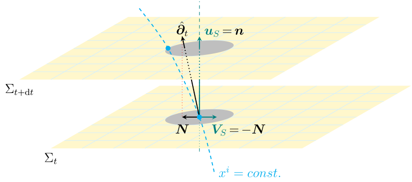
(a) Flow-orthogonal (coordinate velocity)

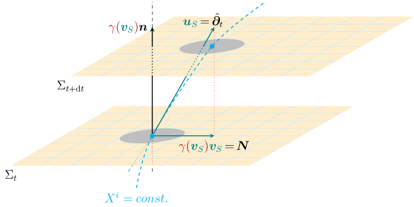
(b) Lagrangian tilted (covariant velocity)

Figure 1: Schematic comparison of the spacetime architecture for (a) Alcubierre and Natário R-Warp, and (b) Lagrangian T-Warp.

We compare the two situations in Figure 1. Figure 1(a) shows two consecutive spatial slices at a lapse distance $N=1$. A coordinate observer keeps its coordinate identity along its tangent vector field $\hat{\bm{\partial}}_{t}$. From this shifted observer the ‘warp bubble’ is observed to move with velocity ${\bm{V}}_{S}$ that compensates the coordinate shift ${\bm{N}}=-{\bm{V}}_{S}$. There is no physical covariant motion of the ‘warp bubble’ that evolves in time along the normal to the hypersurfaces, ${\bm{u}}_{S}={\bm{n}}$, hence does not leave the normal congruence set by the spacetime foliation. Recall that, for the typical description of the warp field in terms of a ‘warp bubble’ with rapidly decaying shift outside of the bubble wall, $\hat{\bm{\partial}}_{t}$ rapidly becomes an Eulerian observer away from the warp field.

On the contrary, in Figure 1(b) the $4$-velocity ${\bm{u}}_{S}$ of the spaceship is tilted with respect to the normal vector $\bm{n}$. This implies a non-vanishing proper velocity $\gamma({\bm{v}}_{S}){\bm{v}}_{S}={\mathrm{d}}{\bm{\ell}}_{S}/{\mathrm{d}}\tau_{S}$ which is the projection of $\bm{u}$ along $\bm{n}$ (cf. (2.3)), $\tensor{h}{{}^{\mu}_{\nu}}u^{\nu}=\gamma({\bm{v}}_{S})v_{S}^{\mu}$. Lapse and shift are chosen such that the spaceship is described in a Lagrangian frame that moves with it: $N^{2}-N^{k}N_{k}=1$, $N=\gamma(\bm{v}_{S})$. Therefore, ${\mathrm{d}}\tau_{S}={\mathrm{d}}t$ (see Section 2.3). Recall that for R-Warp models $N=1=\gamma(\bm{0})$; as a result we also have ${\mathrm{d}}\tau_{S}={\mathrm{d}}\tau_{E}={\mathrm{d}}t$. But, this setting does not involve a non-vanishing covariant velocity.

In this tilted Lagrangian case, a traveller within the spaceship has coordinate velocity ${\bm{V}}_{S}={\bf 0}$ thus keeping its coordinate identity as the coordinate observer in Figure 1(a), but here the vector field $\hat{\bm{\partial}}_{t}$ coincides with the $4$-velocity of the spaceship ${\bm{u}}_{S}$. This has the further advantage that the spaceship is described intrinsically, while in the restricted case the description remains extrinsic.

In both cases the respective proper times equal the coordinate time labeling the spatial leaves (${\mathrm{d}}\tau_{S}={\mathrm{d}}t$). Both figures are extrinsic in the sense that we compare the two situations within the depicted normal congruence. However, the proper time intervals of the Eulerian observers in Figure 1(a) and Figure 1(b) are different: for the restricted case, ${\mathrm{d}}\tau_{E}={\mathrm{d}}t$, but for the tilted cases according to (2.15), ${\mathrm{d}}\tau_{E}=\gamma(\bm{v}_{S})\,{\mathrm{d}}t$.

3 T-Warp: a new concept beyond current proposals

It is evident from our discussion and illustrations that relaxing the imposed restrictions, ${\rm\bf R1}$, ${\rm\bf R2}$ and ${\rm\bf R3}$, discussed in Section 2.2, will allow for the following improvements and suggestion of a new concept for warp drive spacetimes. We name this concept T-Warp for Tilted warp drive as opposed to Restricted warp drive, R-Warp, that obeys all of the above restrictions. T-Warp implies that the restrictions imposed by R-Warp are all relaxed. Tilt is a hierarchically superordered property that subsequently implies, from the existence of a non-vanishing velocity $\bm{v}$, non-vanishing acceleration $\bm{a}$, vorticity $\bm{\omega}$ and spatial curvature in general, while for R-Warp these fields all vanish. Subclasses in which one or more of the physics of T-Warp are neglected can still be considered.

The spatially projected $4$-acceleration will replace the coordinate spatial acceleration, ${\bm{A}}:={\mathrm{d}}\bm{V}/{\mathrm{d}}t$, and the spatially projected covariant vorticity will replace the coordinate spatial vorticity $\bm{\Omega}=\frac{1}{2}\bm{\partial}\times{\bm{V}}$ of the R-Warp concept.

For T-Warp the covariant Lorentz factor becomes singular at the time when the tilted $4$-velocity becomes light-like. Although the spaceship itself is not affected by the extrinsic observations of the left-behind Eulerian observer, the description using the covariant spatial velocity breaks down. Note, however, that the value of the Lorentz factor or of the tilt depends on the relative angle between $\bm{u}$ and $\bm{n}$ at the location of the moving spaceship.

In GR we may not necessarily think of large velocities in terms of $\bm{v}$, as the cosmological example of expanding space, described within a flow-orthogonal setting, shows. Thus, flow-orthogonality is not per se excluding covariant warp effects. It makes physical sense if some restrictions of the R-Warp concept are removed, i.e., keeping ${\rm\bf R1}$, adopting a Lagrangian description for ${\rm\bf R2}$, i.e., using Gaussian normal coordinates ($N=1=\gamma(\bm{0})$, ${\bm{N}}={\bf 0}$), but necessarily relaxing ${\rm\bf R3}$; a flow-orthogonal and covariant warp concept that we may call Lagrangian R1-Warp arises. As an example we mention the possibility to describe propagating gravitational waves in a Lagrangian flow-orthogonal setting [1]. It is an indirect consequence of the equivalence principle allowing to exchange the roles of curvature and acceleration. The restrictions to irrotational and non-accelerating flows, however, remain. Their relaxation, i.e., moving from R1-Warp to T-Warp, may be crucial for warp realizations, as the example below illustrates.

We give an example for interesting new features of T-Warp. As T-Warp allows for acceleration and vorticity, let us quote a relation relating them, taken from [10]: $\omega_{\mu\nu}=u_{[\mu}a_{\nu]}+\partial_{[\mu}u_{\nu]}$. In Lagrangian coordinates, $a_{i}={\mathrm{d}}u_{i}/{\mathrm{d}}t={\mathrm{d}}u_{i}/{\mathrm{d}}\tau_{S}$. Combining this property with $a_{0}=0$, from $a_{\alpha}u^{\alpha}=0$, we can thus write the spatial components of the vorticity, $\omega_{\mu\nu}u^{\nu}=0$, as $\omega_{ij}=u_{[i}a_{j]}+\partial_{[i}u_{j]}$, which shows that vorticity and acceleration are mutually dependent. This relation can be read such that acceleration contributes to vorticity, but in the present context it can also be read such that active generation of vorticity by the spaceship can produce acceleration.

Spatial curvature leads to the image of a spaceship that not only leaves a left-behind Eulerian observer, but also leaves the spatial tangent space of the Eulerian observer to subsequent tangent spaces with tilted unit normal vectors. It is to be analyzed whether this observer will eventually experience the travel of the spaceship as an accelerated motion in space with its subsequent disappearance behind a horizon at a time that depends on acceleration and curvature. A warp concept that assumes that the spaceship is capable of intrinsically warping the space around its rest frames through the correspondence between covariant acceleration (e.g., induced by tilt and covariant vorticity) and spatial curvature would add a truly general-relativistic element.

We believe that the presence of tilt for a physical model of warp is essential. To clarify this point one can think of a warp drive that traverses interplanetary, interstellar or intergalactic distances. The normal congruence would be associated with the frame of the solar system, the galactic plane or the frame of a comoving cosmological background, respectively. In all cases there is a background gravitational field against which a warp drive should act, e.g., to escape the Sun’s gravitational field. (Note that spatial curvature will be important in all cases even if metric perturbations are very small [8].) For R-Warp it is assumed that the background is the Minkowski spacetime and the corresponding warp drive is roving around in a vacuum space, which—as we have shown in Figure 1(a)—represents no physical motion. As a result, a physical proposal for warp drive, we believe, should be based on a covariant formalism and must involve tilted motion if spatial acceleration and vorticity are non-vanishing.

For the understanding of the notion of the warp field or ‘warp bubble’ we may consider the design for the R-Warp concept, where a form function of the bubble comoving with the spaceship may be given as suggested by Alcubierre [2]. The warp field is treated as being part of a continuum, since a velocity field ${\bm{V}}_{S}(t,{\bm{x}})$ is given and the expansion profile is calculated from it. If the warp field were to be a solution of the Einstein equation, initial data had to be prescribed and the ‘warp bubble’ would then be deformed in the course of evolution. For the common realizations of R-Warp, the warp field is assumed to be unaffected along the trajectory of the spaceship. For the Lagrangian T-Warp, given initial data will evolve with a change of the morphology of the Lagrangian boundary of the ‘warp bubble’, described as a compact spatial domain. In this latter case the morphological evolution can be linked to the motion itself [7, Section 3.1.2ff]. Contrary to these descriptions, however, the warp field’s kinematic properties are, taken at face value, phenomena on the scale of the spaceship below the coarse-graining scale of the continuum description of, e.g., interstellar volumes. Kinematic properties may be technically controllable by the spaceship on the scale of the warp field, but in spacetime the warp field would acquire the status of a test particle. Therefore, the scale difference between travel distance and the size of the warp field are also to be understood.

In forthcoming work we shall extend our proposal of T-Warp and employ the Einstein equation to dive deeper into the consequences of the commonly imposed restrictions. By relaxing those restrictions we think that there is much room for resolving previously discussed problems, e.g., the need for exotic energy densities. These problems will appear in a different light within the proposed setting.

Acknowledgments: We thank Doris Folini for valuable remarks on the manuscript, and Asta Heinesen, Jan Ostrowski, Nezihe Uzun for useful discussions. This work is a spin-out from results of a project that has received funding from the European Research Council (ERC) under the European Union’s Horizon 2020 research and innovation programme (grant agreement ERC advanced grant 740021-ARTHUS, PI: TB).

References

References

- [1] F. Al Roumi, T. Buchert, and A. Wiegand. “Lagrangian theory of structure formation in relativistic cosmology. IV. Lagrangian approach to gravitational waves”. Phys. Rev. D 96.12 (2017), p. 123538. arXiv: 1711.01597 [gr-qc].
- [2] M. Alcubierre. “The Warp drive: Hyper-fast travel within general relativity”. Class. Quant. Grav. 11 (1994), pp. L73-L77. arXiv: gr-qc/0009013.
- [3] M. Alcubierre. “Introduction to 3+1 Numerical Relativity”. Oxford University Press, 2008.
- [4] M. Alcubierre and F. S. N. Lobo. “Warp drive basics”. Ed. by F. S. N. Lobo, Wormholes, Warp Drives and Energy Conditions, pp. 1-279. arXiv: 2103.05610 [gr-qc].
- [5] R. L. Arnowitt, S. Deser, and C. W. Misner. “Republication of: The Dynamics of general relativity”. Gen. Relativ. Gravit. 40 (2008), pp. 1997-2027. arXiv: gr-qc/0405109.
- [6] C. V. D. Broeck. “A ‘warp drive’ with more reasonable total energy requirements”. Class. Quantum Grav. 16 (1999), pp. 3973-3979. arXiv: gr-qc/9905084.
- [7] T. Buchert. “Dark Energy from Structure: A Status Report”. Gen. Relativ. Gravit. 40 (2008), pp. 467-527. arXiv: 0707.2153 [gr-qc].
- [8] T. Buchert, G. F. R. Ellis, and H. van Elst. “Geometrical order-of-magnitude estimates for spatial curvature in realistic models of the Universe”. Gen. Relativ. Gravit. 41 (2009), pp. 2017-2030. arXiv: 0906.0134 [gr-qc].
- [9] T. Buchert, P. Mourier, and X. Roy. “Cosmological backreaction and its dependence on spacetime foliation”. Class. Quant. Grav. 35.24 (2018), 24LT02. arXiv: 1805.10455 [gr-qc].
- [10] T. Buchert, P. Mourier, and X. Roy. “On average properties of inhomogeneous fluids in general relativity III: general fluid cosmologies”. Gen. Relativ. Gravit. 52.3 (2020), p. 27. arXiv: 1912.04213 [gr-qc].
- [11] T. M. Davis and C. H. Lineweaver. “Expanding confusion: common misconceptions of cosmological horizons and the superluminal expansion of the universe”. Publ. Astron. Soc. Austral. 21 (2004), p. 97. arXiv: astro-ph/0310808.
- [12] G. F. R. Ellis and T. Rothman. “Lost horizons”. Am. J. Phys. 61.10 (1993), pp. 883-893.
- [13] H. Friedrich. “Evolution equations for gravitating ideal fluid bodies in general relativity”. Phys. Rev. D 57 (1998), pp. 2317-2322.
- [14] R. Geroch. “Faster than light?”, Advances in Lorentzian geometry, pp. 59-69. Amer. Math. Soc., Providence, RI, 2011.
- [15] E. Gourgoulhon. Formalism in General Relativity. Bases of numerical relativity. Vol. 846. Lecture Notes in Physics. Berlin: Springer, 2012. arXiv: gr-qc/0703035.
- [16] E. Gourgoulhon. Special Relativity in General Frames: From Particles to Astrophysics. 1st ed. Graduate Texts in Physics. Springer Berlin, Heidelberg, 2013, pp. XXX, 784.
- [17] A. Heinesen, P. Mourier, and T. Buchert. “On the covariance of scalar averaging and backreaction in relativistic inhomogeneous cosmology”. Class. Quant. Grav. 36 (2019), p. 075001. arXiv: 1811.01374 [gr-qc].
- [18] C. Helmerich, J. Fuchs, and J. F. Agnew. “Numerical Optimization of Warp Drive Geometries”, AIAA Propulsion and Energy 2021 Forum .
- [19] C. Helmerich, J. Fuchs, A. Bobrick, L. Sellers, S. Dangelo, G. Martire, and J. F. Agnew. “Warp Factory: A Numerical Toolkit for the Analysis and Optimization of Warp Drive Geometries”, AIAA SCITECH 2023 Forum .
- [20] S. V. Krasnikov. “Hyperfast travel in general relativity”. Phys. Rev. D 57 (1998), pp. 4760-4766. arXiv: gr-qc/9511068.
- [21] M. S. Morris and K. S. Thorne. “Wormholes in spacetime and their use for interstellar travel: A tool for teaching general relativity”. Am. J. Phys. 56.5 (1988), pp. 395-412.
- [22] D. Mumford. “Ruminations on Cosmology and Time”. Not. Am. Math. Soc. 68 (2021), pp. 1715-1725.
- [23] J. Natário. “Warp drive with zero expansion”. Class. Quant. Grav. 19 (2002), pp. 1157-1166. arXiv: gr-qc/0110086.
- [24] W. Rindler. Essential Relativity: Special, General, and Cosmological. 1st ed. Springer New York, NY, 1969, pp. XIII, 319.
- [25] R. K. Sachs and H.-H. Wu. General Relativity for Mathematicians. 1st ed. Graduate Texts in Mathematics. Springer New York, NY, 1977, pp. XII, 292.
- [26] J. Santiago, S. Schuster, and M. Visser. “Generic warp drives violate the null energy condition”. Phys. Rev. D 105.6 (2022), p. 064038. arXiv: 2105.03079 [gr-qc].
- [27] L. Smarr and J. W. York Jr. “Kinematical conditions in the construction of space-time”. Phys. Rev. D 17 (1978), pp. 2529-2551.
- [28] M. Visser. Lorentzian Wormholes. From Einstein to Hawking. 1st ed. Melville, NY: American Institute of Physics, 1996, pp. XXV, 412.
- [29] H. White. “A Discussion of Space-Time Metric Engineering”. Gen. Relativ. Gravit. 35 (2003), pp. 2025-2033.
- [30] H. White, P. March, N. Williams, and W. ONeill. “Eagleworks laboratories: advanced propulsion physics research”, JANNAF Joint Propulsion Meeting.