Sum-of-norms regularized Nonnegative Matrix Factorization

Abstract

When applying nonnegative matrix factorization (NMF), generally the rank parameter is unknown. Such rank in NMF, called the nonnegative rank, is usually estimated heuristically since computing the exact value of it is NP-hard. In this work, we propose an approximation method to estimate such rank while solving NMF on-the-fly. We use sum-of-norm (SON), a group-lasso structure that encourages pairwise similarity, to reduce the rank of a factor matrix where the rank is overestimated at the beginning. On various datasets, SON-NMF is able to reveal the correct nonnegative rank of the data without any prior knowledge nor tuning.

SON-NMF is a nonconvx nonsmmoth non-separable non-proximable problem, solving it is nontrivial. First, as rank estimation in NMF is NP-hard, the proposed approach does not enjoy a lower computational complexity. Using a graph-theoretic argument, we prove that the complexity of the SON-NMF is almost irreducible. Second, the per-iteration cost of any algorithm solving SON-NMF is possibly high, which motivated us to propose a first-order BCD algorithm to approximately solve SON-NMF with a low per-iteration cost, in which we do so by the proximal average operator. Lastly, we propose a simple greedy method for post-processing.

SON-NMF exhibits favourable features for applications. Beside the ability to automatically estimate the rank from data, SON-NMF can deal with rank-deficient data matrix, can detect weak component with small energy. Furthermore, on the application of hyperspectral imaging, SON-NMF handle the issue of spectral variability naturally.

Keywords: nonnegative matrix factorization, rank, regularization, sum-of-norms, nonsmooth nonconvex optimization, algorithm, proximal gradient, proximal average, complete graph

1 Introduction

Nonnegative Matrix Factorization (NMF)

We denote NMF($\bm{M},r$) [1, 2] the following problem: given a matrix $\bm{M}\in\mathbb{R}^{m\times n}_{+}$, find two factor matrices $\bm{W}\in\mathbb{R}^{m\times r}_{+}$ and $\bm{H}\in\mathbb{R}^{r\times n}_{+}$ such that $\bm{M}=\bm{W}\bm{H}$. NMF describes a cone: $\bm{M}$ is a point cloud (of $n$ points) in $\mathbb{R}^{m}_{+}$, contained in a polyhedral cone generated by the $r$ columns of $\bm{W}$ with nonnegative weights encoded in $\bm{H}$, where $H_{ij}$ represents the contribution of column $\bm{w}_{i}$ in representing the data column $\bm{m}_{j}$, e.g., see [3, Fig.1].

Nonnegative rank

Let $r=\textrm{rank}_{+}(\bm{M})$ denotes the nonnegative-rank of a matrix, where $r$ represents the minimal number of nonnegative rank-1 components required to represent $\bm{M}$ [4, Section 4], [2, Section 3], i.e.,

$$\texttt{NMF}(\bm{M},r)\leavevmode\nobreak\ :\leavevmode\nobreak\ \bm{M}=\bm{W}\bm{H}=\begin{bmatrix}\bm{w}_{1}\dots\bm{w}_{r}\end{bmatrix}\begin{bmatrix}\bm{h}^{1}\\ \vdots\\ \bm{h}^{r}\end{bmatrix}=\bm{w}_{1}\bm{h}^{1}+\dots+\bm{w}_{r}\bm{h}^{r}=\sum_{\ell=1}^{r}\bm{w}_{\ell}\bm{h}^{\ell},\leavevmode\nobreak\ \leavevmode\nobreak\ \bm{w}_{\ell}\geq\bm{0},\bm{h}^{\ell}\geq\bm{0},$$ (1)

where $\bm{w}_{j}$ is the $j$th column of $\bm{W}$, and $\bm{h}^{j}$ is the $j$th row of $\bm{H}$. Here $\bm{w}_{j}\bm{h}^{j}$ is the $j$th rank-1 factor in $\bm{W}\bm{H}$.

$r$ is important

Parameter $r$ controls the model complexity of NMF and plays a critical role in data analysis. In signal processing [5], $r$ represents the number of sources in a audio. If $r$ is over-estimated, over-fitting occurs where the over-estimated component in the models the noise (e.g. piano mechanical noise [6, Section 4.2]) instead of meaningful information.

$r$ is unknown

Generally $r$ is unknown, finding $r$ in NMF($\bm{M},r$) for $\textrm{rank}_{+}(\bm{M})\geq 3$ is NP-hard [7]. In many cases $\textrm{rank}(\bm{M})$ and/or $\textrm{rank}_{+}(\bm{M})$ are small since $\bm{M}$ is approximately low rank [8] and/or low nonnegative-rank [2, Section 9.2]. Many heuristics have been proposed to find $r$ in the literature: beside trial-and-error, the two main groups of methods for finding $r$ are stochastic/information-theoretic and algebraic/deterministic. The first group includes Bayesian method [9], cophenetic correlation coefficient [10] and minimum description length [11]. The second group includes fooling set [12] and $f$-vector in combinatorics [13]. See [2, Section 3] for a summary on the algebra of $\textrm{rank}_{+}$.

In this work, we focus on approximately solving NMF($\bm{M},r$), without tuning nor knowing $r$ in advance. This is achieved by imposing a “rank penalty” on NMF. Instead of using the nuclear norm nor the rank itself as a penalty term, we consider a clustering regularizer called Sum-of-norms (SON): we propose SON-NMF to “relax” the assumption of knowing $r$. Before we introduce SON-NMF, we first review the SON term.

Matrix $\ell_{p,q}$-norm

The $\ell_{p,q}$-norm of a matrix $\bm{X}\in\mathbb{R}^{m\times n}$ is defined as

$$\|\bm{X}\|_{p,q}\leavevmode\nobreak\ \coloneqq\leavevmode\nobreak\ \left(\sum_{j=1}^{n}\Bigg{(}\sqrt[p]{\sum_{i=1}^{m}X_{ij}^{p}}\Bigg{)}^{q}\right)^{\frac{1}{q}}\leavevmode\nobreak\ =\leavevmode\nobreak\ \left\|\begin{bmatrix}\|\bm{x}_{1}\|_{p}\\ \vdots\\ \|\bm{x}_{n}\|_{p}\end{bmatrix}\right\|_{q},$$

where in the last equality we take the $p$-norm on columns followed by taking $q$-norm on the resulting vector. A popular choice of the $\ell_{p,q}$-norm is $\ell_{2,1}$-norm, used in multiple measurement vector problem [14], sparse coding [15] and robust NMF [16].

Sum-of-norms (SON)

We define the SON of a matrix $\bm{X}$ as the $\ell_{2,1}$-norm of $P(\bm{X})$, where $\bm{X}\mapsto P(\bm{X})$ is all the pairwise difference $\bm{x}_{i}-\bm{x}_{j}$. As $\|\bm{x}_{i}-\bm{x}_{j}\|_{2}=\|\bm{x}_{j}-\bm{x}_{i}\|_{2}$, there are $\frac{n^{2}-n}{2}$ terms in SON of $\bm{X}$. In this work we propose to use SON${}_{2,1}(\bm{W})$ as a regularizer for the NMF, to be presented in the next section. Below we give remarks on SON${}_{2,q}(\bm{W})$ with other choices of $q$.

• SON${}_{2,0}(\bm{W})$ with $q=0$: it is trivial that $\textrm{rank}(\bm{W})\leq\textrm{SON}_{2,0}(\bm{W})$ because the set of linearly independent vectors is a subset of the set of unequal pair of vectors. Next, by the combinatorial nature of $\ell_{0}$-norm, minimizing $\textrm{SON}_{2,0}(\bm{W})$ is NP-hard and its complexity scales with $r$, so SON${}_{2,0}(\bm{W})$ is computationally unfavourable to NMF for applications with a large $r\approx(m,n)$, which is the case in this work.

• SON${}_{2,2}(\bm{W})$ with $q=2$: it is the Frobenius norm of $P(\bm{W})$ by definition. This SON has been used in graph-regularized NMF [17], which is different from (SON-NMF) for two reasons: 1. the graph regularizer is a weighted-squared-$\textrm{SON}_{2,2}$ norm which is everywhere differentiable, which is not the case for SON${}_{2,1}(\bm{W})$, and 2. SON${}_{2,2}(\bm{W})$ does not induce sparsity while SON${}_{2,1}(\bm{W})$ does.

• SON${}_{2,\infty}(\bm{W})$ with $q\rightarrow\infty$: this term focuses on the pair $(\bm{w}_{i},\bm{w}_{j})$ that is mutually furthest away from each other, and ignoring the rest. This is unfavourable for removing the redundant $\bm{w}_{j}$ in NMF for this work.

We are now ready to introduce SON-NMF.

SON-NMF

In this work we propose to regularize NMF by $\textrm{SON}_{2,1}(\bm{W})=\displaystyle\|P(\bm{W})\|_{2,1}=\sum_{i\neq j}\|\bm{w}_{i}-\bm{w}_{j}\|_{2}$:

$$\operatorname*{\textrm{argmin}\,}_{\bm{W},\bm{H}}\,F(\bm{W},\bm{H})\leavevmode\nobreak\ \coloneqq\leavevmode\nobreak\ \dfrac{1}{2}\|\bm{W}\bm{H}-\bm{M}\|_{F}^{2}+\lambda\sum_{i\neq j}\|\bm{w}_{i}-\bm{w}_{j}\|_{2}+\gamma\sum_{i}\|\max\{-\bm{w}_{i},\bm{0}\}\|_{1}+\iota_{\Delta^{r}}(\bm{H}),$$ (SON-NMF)

where $\frac{1}{2}\|\bm{M}-\bm{W}\bm{H}\|_{F}^{2}:\mathbb{R}^{m\times n}\times\mathbb{R}^{m\times r}\times\mathbb{R}^{r\times n}\rightarrow\mathbb{R}$ is a smooth nonconvex data fitting term, the constants $\lambda>0$ and $\gamma>0$ are parameters, the functions $\sum_{i}\|\max\{-\bm{w}_{i},\bm{0}\}\|_{1}$ and $\iota_{\Delta^{r}}(\bm{H})=\sum_{j}\iota_{\Delta^{r}}(\bm{h}_{j})$ are nonsmooth lower-semicontinuous proper convex that represent model constraints: respectively the nonnegativity of $\bm{w}_{j}$ (i.e., $\bm{W}\geq\bm{0}$) and $\bm{h}_{j}$ is inside $r$-dimensional unit simplex (i.e., $\bm{H}$ is element-wise nonnegative and $\bm{H}^{\top}\bm{1}_{r}\leq\bm{1}_{n}$ where $\bm{1}_{r}\in\mathbb{R}^{r}$ denotes vector of ones). Note that in (SON-NMF) we use the penalty $\sum_{i}\|\max\{-\bm{w}_{i},\bm{0}\}\|_{1}$, which is equivalent to the nonnegativity constraint $\bm{W}\geq\bm{0}$ for sufficiently large $\lambda$, to be explained in section 4. We defer to the end of this section for the definition of symbols used in (SON-NMF).

Interpretation of SON: encouraging multicollinearity and rank-deficiency for NMF

The SON term encourages the pairwise difference in $\|\bm{w}_{i}-\bm{w}_{j}\|_{2}$ to be small, possibly resulting in multicollinearity in the matrix $\bm{W}$. Note that in traditional regression models, multicollinearity is strongly discouraged due to its negative statistical effect on the variables [18]. In this work, we intentionally encourage the multicollinearity of $\bm{W}$, for the sake of encouraging rank deficiency in $\bm{W}$ in order to reduce an overestimated rank for rank-estimation. I.e., SON-NMF can be seen as the ordinary NMF model under a multicollinearity regularizer where the rank of $\bm{W}$ at the first iteration is overestimated and then it is the job of the regularizer to reduce the overestimated rank of $\bm{W}$ to the correct value in the algorithmic process.

There is a “price to pay” for such multicollinearity. If $\bm{W}$ is near-multicollinear, the conditional number of $\bm{W}$ is large so $\bm{W}^{\top}\bm{W}$ is ill-conditioned, negatively impacting the process of updating $\bm{H}$. See the discussion in Section 3.

Contributions

We introduce a new problem (SON-NMF) with the following contributions.

• Empirically rank-revealing.   On synthetic and real-world datasets, we empirically show that model (SON-NMF), free from tuning the rank $r$, will itself find the correct $r$ in the data automatically when $r$ is overestimated. This is due to the sparsity-inducing property of the $\ell_{2,1}$ norm in SON_2,1.

  • Rank-deficient compatibility. SON-NMF can work with rank-deficient problem, i.e., on data matrix with the true rank smaller than the over overestimated parameter $r$. This has two advantages. First, it means the model prevents over-fitting. Second, compared with existing NMF models such as the minimum-volume NMF [19, 5] (see below) which was shown to exhibit [3] rank-finding ability, SON-NMF is applicable to rank-deficient matrix.

• Irreducible computational complexity. As computing $\textrm{rank}_{+}$ is NP-hard, the SON approach, as a “work-around” approach to estimate $\textrm{rank}_{+}$, cannot enjoy a lower complexity. We prove that (Theorem 1) the complexity of the SON term is almost irreducible. Precisely, we show that in the best case, to recover the $r^{*}$ columns of the true $\bm{W}^{*}$ using $\bm{W}$ obtained from SON-NMF with a rank $r>r^{*}$, we cannot reduce the complexity of the SON term from $r(r-1)/2$ to below $r(r-\lceil r/r^{*}\rceil)/2$.

• Fast algorithm by proximal-average.   Solving (SON-NMF) is not trivial: the $\bm{W}$-subproblem is nonsmooth non-separable and non-proximable, meaning that proximal-based methods [20, 21, 22, 23, 24] cannot efficiently solve the problem. When dealing with non-proximal problem, dual approach like Lagrange multiplier and ADMM are usually used, however SON-NMF has $\mathcal{O}(r^{2})$ pairs of non-proximal terms and such complexity is irreducible (Theorem 1), the dual methods and second-order methods are inefficient since they have a very high per-iteration cost. We propose a low-cost proximal average [25] based on the Moreau-Yosida envelop [26].

We review the literature in the next paragraphs, on the background and the motivation of this work.

Review of NMF: minimum-volume and rank-deficiency

SON-NMF has linkage to minvol NMF [19, 27]. Recently it has been observed in [3] that when using volume regularization in the form of $\log\det(\bm{W}^{\top}\bm{W}+\delta\bm{I}_{r})$, minvol NMF on rank deficient matrix $\bm{M}$ (i.e., overestimating the $r$ parameter) has the ability to zeroing out extra components in $\bm{W},\bm{H}$. This has also been observed in audio blind source separation [5], where a rank-7 factorization is used on a dataset with 3 sources, the minvol NMF is able to set the redundant components to zero. I.e., minvol NMF can automatically select the model order $r$. However minvol NMF is not suitable for rank-deficient $\bm{W}$: we have $\log\det(\bm{W}^{\top}\bm{W})=\log 0=-\infty$ if $\delta=0$. Even if $\delta\neq 0$, the rank-deficient $\bm{W}$ provide no information in the logdet term. Furthermore, in the work [5] on using an overestimated rank in minvol NMF, it is the redundant components in matrix $\bm{H}$ set to zero instead of $\bm{W}$. We remark that it is the rank-revealing observation of minvol NMF motivated the first author to propose SON-NMF.

Review of clustering

SON was proposed in [28, 29] on clustering. Due to the interpretation that minimizing SON$(\bm{W})$ will force the pairwise difference $\bm{w}_{i}-\bm{w}_{j}$ to be small, SON is also called “fusion penalty” [30]. Later [31] considered SON with $0<p<1$, and recently [32] showed that SON clustering can provably recover the Gaussian mixture under some assumptions. SON_2,0 is also used in graph trend filtering [33]. We remark that these works are different from SON-NMF: they are single-variable problem, and NMF is a bi-variate nonconvex problem with nonnegativity constraints.

SON solution approaches

The approach we proposed to solve the SON problem is different from the existing approaches such as quadratic programming with convex hull [28], active-set [30], interior-point method [29], trust-region with smoothing [31], Lagrange multiplier [34, 12.3.8] and semi-smooth Newton’s method [35]. These approaches are all proposed for single-variable clustering (i.e., $\bm{W}$ only) with no nonnegativity constraint. What we proposed is to makes use of proximal average [26, 25] which is computationally cheap to compute (with a per-iteration cost $\mathcal{O}(m)$ where $m$ is the dimension of $\bm{w}_{j}$) for SON and thus lowering the per-iteration cost. All the method mentioned above are either unable to solve the SON problem on $\bm{W}$ with nonnegativity, or having a higher per-iteration cost. See details in section 4.

History: the geometric median and the Fermat-Torricelli-Weber problem and

Although SON is proposed in 2000s [28, 30, 29], it is closely related to an old problem known as the Fermat-Torricelli-Weber problem [36, 37], [34, Example 3.66], also known as the geometric median. We note that the analysis of geometric median does not apply to SON-NMF, but it provides a geometric interpretation: SON-NMF produces a $r^{*}$-cluster of points with the smallest geometric median to the dataset.

Rank estimation in NMF

Existing works on rank estimation for NMF is not applicable in the setting of this paper. The algebraic methods like fooling sets [12] and $f$-vector [13] only give a loose bound on $\textrm{rank}_{+}(\bm{M})$ and are being expensive to implement. The statistical approaches [9, 11, 10] assume $\bm{W}$ and $\bm{H}$ follows some pre-defined distributions, or require on heavy post-processing. SON-NMF has none of these assumptions, restrictions nor post-processing.

A “drawback” of SON-NMF

Finding the $\textrm{rank}_{+}$ in NMF is NP-hard, the search space of $r$ in NMF is the set of natural number $\mathbb{N}$, which has a cardinality of countably infinite. In SON-NMF we do not need to estimate the rank $r$, but we are required to provide a regularization parameter $\lambda$, in which its search space is the set of nonnegative real $\mathbb{R}_{+}$. By Cantor’s diagonal argument [38], the cardinality of real number is uncountably infinite. Hence, it seems in SON-NMF we are moving from NMF with a search space $\mathbb{N}$ to SON-NMF with much larger search space $\mathbb{R}_{+}$, and thus SON-NMF is even more difficult to solve than the already NP-hard NMF. We remark that this is true theoretically, however it is not a problem practically because many datasets are hierarchically clustered in the latent space, and thus a simple tuning of $\lambda$ can be used on SON-NMF to find the true rank.

Paper organization

We provide theory of SON-NMF in section 2. We present how to solve SON-NMF in section 3 and section 4. We give experimental results in section 5. We conclude in section 6.

Notation

The notation “$\{x,y\}$ denotes $\{X,Y\}$” means that we denote the object $X$ by the symbol $x$ and the object $Y$ by the symbol $y$ respectively (resp.). We use the symbols $\{\mathbb{R},\mathbb{R}_{+},\overline{\mathbb{R}},\mathbb{R}^{m},\mathbb{R}^{m\times n}\}$ to denote $\{$reals, nonnegative reals, extended reals, $m$-dimensional reals, $m$-by-$n$ reals$\}$, we use $\{$lowercase italic, bold lowercase italic, bold uppercase letters$\}$ to represent $\{$scalar, vector, matrix$\}$. Given a matrix $\bm{M}$, we denote $\{\bm{m}^{i},\bm{m}_{j}\}$ the $\{i$th row, $j$th column$\}$ of $\bm{M}$. Given a convex set $C\subset\mathbb{R}^{n}$, the indicator function of $C$ at $\bm{x}$ is defined as $\iota_{C}(\bm{x})=0$ if $\bm{x}\in C$ and $\iota_{C}=+\infty$ if $\bm{x}\notin C$, and $\textrm{proj}_{C}(\bm{x})$ denotes the projection of a point $\bm{x}$ onto $C$. The projection of $\{\bm{v}\in\mathbb{R}^{n},\bm{V}\in\mathbb{R}^{m\times n}\}$ onto the nonnegative orthant $\{\mathbb{R}^{n}_{+},\mathbb{R}^{m\times n}_{+}\}$ is denoted by the element-wise max operator $\{[\bm{v}]_{+},[\bm{V}]_{+}\}$. Lastly $\Delta^{r}\in\mathbb{R}^{r}$ denotes the unit simplex and $\bm{1}_{r}\in\mathbb{R}^{r}$ is the vector of 1s.

Remark.

Note that the constraint on $\bm{H}$ removes the scaling ambiguity of the factorization. That is, there do not exists a diagonal matrix $\bm{D}$ that $\bm{M}=\bm{W}_{1}\bm{H}_{1}=(\bm{W}_{1}\bm{D})(\bm{D}^{-1}\bm{H}_{1})\eqqcolon\bm{W}_{2}\bm{H}_{2}$ such that $\bm{W}_{1}\neq\bm{W}_{2}$ and $\bm{H}_{1}\neq\bm{H}_{2}$.

2 Theory of SON-NMF

In this section we provide theories of SON_2,1-NMF. First we give a closer look at SON_2,1, then we give the motivation why one would like to reduce the complexity of SON_2,1, next we give a bound showing that such complexity is irreducible. Lastly we discuss a greedy method utilising the property of SON_2,1.

2.1 SON_2,1 has $r^{2}$ terms and its minimum occurs at maximal cluster-imbalance

Let $\bm{X}=[\bm{x}_{1},\bm{x}_{2},\cdots]$ has five columns. Let vec denotes vectorization. The pair-wise difference $P$ in SON can be expressed as

$$P(\bm{X})\leavevmode\nobreak\ =\leavevmode\nobreak\ \bm{A}\textrm{vec}(\bm{X})\leavevmode\nobreak\ =\leavevmode\nobreak\ \begin{bmatrix}\bm{I}&-\bm{I}&&\cdots\\ \bm{I}&&-\bm{I}&\cdots\\ \vdots&\vdots&\vdots&\ddots\end{bmatrix}\begin{bmatrix}\bm{x}_{1}\\ \bm{x}_{2}\\ \vdots\\ \end{bmatrix}\leavevmode\nobreak\ =\leavevmode\nobreak\ \begin{bmatrix}\bm{x}_{1}-\bm{x}_{2}\\ \bm{x}_{1}-\bm{x}_{3}\\ \vdots\end{bmatrix},$$

which has $5^{2}-5=20$ pairs of $(\bm{x}_{i},\bm{x}_{j})$. In general, suppose $\bm{X}$ has $r$ columns, then the term $P(\bm{X})$ contains $r(r-1)$ pairs of $(\bm{x}_{i},\bm{x}_{j})$. By symmetry $\|\bm{x}_{i}-\bm{x}_{j}\|_{2}=\|\bm{x}_{j}-\bm{x}_{i}\|_{2}$, we drop the repeated terms so SON effectively has $r(r-1)/2$ distinct pairs. We now switch to the language of graph theory. Denote $G(V,E)$ a simple undirected unweighted graph of $|V|$ nodes and $|E|$ edges. Let $K_{r}$ be complete graph of $r$ nodes. Then SON${}_{2,1}(\bm{X})=\sum\|\bm{x}_{i}-\bm{x}_{j}\|_{2}$ for $(i,j)\in K_{r}$. As $|E(K_{r})|=r(r-1)/2$, so SON_2,1 has $\mathcal{O}(r^{2})$ terms.

Back to the example of $\bm{X}$ with five columns. Let $\bm{X}$ be a rank-3 matrix with three clusters with centers $\bm{c}_{1},\bm{c}_{2},\bm{c}_{3}$ as $\bm{X}=[\bm{x}_{1}\leavevmode\nobreak\ |\leavevmode\nobreak\ \bm{x}_{2}\leavevmode\nobreak\ |\leavevmode\nobreak\ \bm{x}_{3}\leavevmode\nobreak\ \bm{x}_{4}\leavevmode\nobreak\ \bm{x}_{5}]=[\bm{c}_{1}\leavevmode\nobreak\ |\leavevmode\nobreak\ \bm{c}_{2}\leavevmode\nobreak\ |\leavevmode\nobreak\ \bm{c}_{3}\leavevmode\nobreak\ \bm{c}_{3}\leavevmode\nobreak\ \bm{c}_{3}]$ so SON${}_{2,1}(\bm{X})=\|\bm{c}_{1}-\bm{c}_{2}\|_{2}+3\|\bm{c}_{1}-\bm{c}_{3}\|_{2}+3\|\bm{c}_{2}-\bm{c}_{3}\|_{2}$. We show the graph $K_{5}$ and the pair-wise difference below.

	1	2	3	4	5
1	0	$\bm{c}_{1}-\bm{c}_{2}$	$\bm{c}_{1}-\bm{c}_{3}$	$\bm{c}_{1}-\bm{c}_{3}$	$\bm{c}_{1}-\bm{c}_{3}$
2		0	$\bm{c}_{2}-\bm{c}_{3}$	$\bm{c}_{2}-\bm{c}_{3}$	$\bm{c}_{2}-\bm{c}_{3}$
3			0	0	0
4				0	0
5					0

Now we generalize: let $\bm{X}$ with $r$ columns has $r^{*}\leq r$ clusters $C_{1},\cdots,C_{r*}$ with centers $\bm{c}_{1},\cdots,\bm{c}_{r^{*}}$. Let $|C_{i}|$ denotes the cluster size of $C_{i}$. By $|C_{1}|+\cdots+|C_{r^{*}}|=r$ we have

$$\begin{array}[]{rcl}\text{SON}_{2,1}(\bm{X})&=&\displaystyle\sum_{(i,j)\in K_{r}}|C_{i}||C_{j}|\big{\|}\bm{c}_{i}-\bm{c}_{j}\big{\|}_{2}\\ &\leq&\displaystyle\bigg{(}\max_{i\in[r]}|C_{i}|\bigg{)}\bigg{(}\max_{i,j}\big{\|}\bm{c}_{i}-\bm{c}_{j}\big{\|}_{2}\bigg{)}\sum_{(i,j)\in K_{r}}|C_{j}|\leq\bigg{(}\max_{i\in[r]}|C_{i}|\bigg{)}\bigg{(}\max_{i,j}\big{\|}\bm{c}_{i}-\bm{c}_{j}\big{\|}_{2}\bigg{)}\,r,\end{array}$$

giving a stopping criterion for the algorithm: we know $r$ as an input, so we just need to track the product $\displaystyle\big{(}\max_{i\in[r]}|C_{i}|\big{)}\big{(}\max_{i,j}\big{\|}\bm{c}_{i}-\bm{c}_{j}\big{\|}_{2}\big{)}$ for convergence. Furthermore, from the inequality we can focus on the cluster size instead of the norm $\|\bm{c}_{i}-\bm{c}_{j}\|_{2}$, and arrive at the following Lemma that characterizes the theoretical minimum of SON_2,0 as a proxy of SON_2,1.

Lemma 1 (Maximal cluster-imbalance gives the minimum of SON-2-0).

For a $n$-column matrix $\bm{X}$ with $K$ clusters $C_{1},\dots,C_{K}$ where $\bm{x}_{i}\in C_{i}$ all takes the centroid $\bm{c}_{i}$, then $\textrm{SON}_{2,0}(\bm{X})=\sum_{i,j}|C_{i}||C_{j}|$ achieves the lowest value if a cluster takes $n-K+1$ columns in $\bm{X}$ and the other $K-1$ clusters have a unit cluster size.

Proof.

Trivial by using the fact $|C_{1}|+...+|C_{K}|=K$ with some inequality manipulations. ∎

Remarks of Lemma 1

1. As $\ell_{1}$-norm is a tight convex relaxation of the $\ell_{0}$-norm (over the unit ball), then Lemma 1 on the SON_2,0 term gives a theoretical minimum for the SON_2,1 term (if the input matrix is in a unit ball).

2. For any cluster $C_{i}$ the smallest cluster size is $1$ and it is impossible for the SON_2,0 term (similarly for the SON_2,1 term) to “miss” a weak component in the data, if exist. This is observed in the experiment, see Fig. 7 and Fig. 5 in Section 5. Furthermore, if the centers $\bm{c}_{i}$ have similar distance to each other: $\|\bm{c}_{i}-\bm{c}_{j}\|_{2}\approx\|\bm{c}_{j}-\bm{c}_{k}\|_{2}$, then maximal cluster-imbalance will occur in the application. See Fig. 3, Fig. 4, Fig. 6, Fig. 7 in Section 5

2.2 SON complexity is irreducible

We now see that SON has $\mathcal{O}(r^{2})$ terms. In the application, we are using a large input rank $r$ (possibly as large as the data-size $m,n$) in the SON-NMF to estimate the true rank $r^{*}$ of the data. This means the SON term has a high computational complexity and thus is impractical. So it natural to ask whether it is possible to reduce the complexity of the SON term by removing some edges in $K_{r}$, so that we can cut the per-iteration cost of running SON-NMF, while retaining some recovery performance of SON-NMF. We gives a negative result to this idea (Theorem 1). That is, the complexity of SON term is almost irreducible.

Remark.

There are works on the literature with a similar idea. For example, [35, page 2] mentioned approaches using $k$-nearest neighbors. We remark that these are data-dependent approaches that use the data to learn a graph structure for reducing the complexity of the SON term. Our focus here is different. We are focusing on the possibility of reducing the complexity of the SON term purely from the graph perspective, independent of data. I.e., we are interested in finding the possible sparsest subgraph that such a reduced-SON is the “functionally the same” as the full-SON, and Theorem 1 below is saying that such sparsest subgraph basically does not exist.

We first give notation. Let $r^{*}$ be the true NMF rank of $\bm{W}$. For a graph $G(V,E)$, let $u,v$ be two nodes in $V$ of $G$ that there is an edge between them, i.e., $(u,v)\in E$. The notation $G\setminus(u,v)$ denotes the subgraph of $G$ removing the edge $(u,v)$. The notion of graph partition of $G$ is the set of subgraphs $S_{1},S_{2},\cdots$ of $G$ where $V(S_{i})$ are the partition of $V(G)$ that $V(S_{i})$ are mutually exclusive sets. Now, we have a trivial fact.

Lemma 2.

Let $\bm{W}$ has the true NMF rank $r^{*}$. Then the graph generated by the columns of $\bm{W}$ must have the following property. For every possible partitioning of the nodes of the graph into $r^{*}$ subgraphs, each subgraph needs to be connected.

This lemma can be proved easily by contradiction. Now we have the following lemma.

Lemma 3.

The only graph that satisfies the condition of Lemma 2 is the complete graph.

Proof.

Let $G$ be a graph whose nodes correspond to columns of $\bm{W}$. Suppose that some particular edge $(u,v)$ is omitted from $G$. Then it is possible that the ‘true’ partition is: $(u,v)$ is one partition, while the remaining nodes of $G\setminus(u,v)$ are divided arbitrarily among the other $r^{*}-1$ partitions. In this case, $u$ and $v$ are not connected by edges except through $G\setminus(u,v)$. Since $u,v$ were arbitrary, the conclusion is that no edge can be omitted from $G$. ∎

The lemma means that apart from the complete graph, we cannot consider other graph structure. The following theorem quantify the amount of edge we can remove from the complete graph.

Theorem 1.

Let $(\bm{W}^{*},\bm{H}^{*})=\texttt{NMF}(\bm{M},r^{*})$ be the true solution, and let $(\bm{W},\bm{H})=\texttt{SON-NMF}(\bm{M},r)$ with $r\geq r^{*}$ be another solution. If we want to recover $\bm{W}^{*}$ using $r^{*}$ clusters of the $r$ columns of $\bm{W}$, we cannot reduce the number of pairwise difference term $\|\bm{w}_{i}-\bm{w}_{j}\|_{2}$ in SON below $r(r-\lceil r/r^{*}\rceil)/2$.

Proof.

We construct a simple undirected unweighted graph $G(V,E)$ with $|V|=r$ nodes where each node $v\in V$ represents a vector $\bm{w}_{i}$ of $\bm{W}$ produced by $\texttt{SON-NMF}(\bm{M},r)$. Here an edge $e(u,v)$ denotes the pairwise difference $\|\bm{w}_{i}-\bm{w}_{j}\|_{2}$. Now, recovering $\bm{W}^{*}$ by $\bm{W}$ with fewer terms in the SON regularizer can be translated as:

$$\begin{array}[]{l}\text{we can identify $r^{*}$ disjoint clusters in $G$ with $|V|=r$ using a subgraph of $K_{r}$ with fewer edges.}\end{array}$$ (2)

We are going to show that the statement (2) is true, and at best such an improvement is from $r(r-1)/2$ to $r(r-\lceil r/r^{*}\rceil)/2$.

Assuming, in the best case that, each of these $r^{*}$ columns of $\bm{W}^{*}$ is associated with exactly $\lceil r/r^{*}\rceil$ nodes in $\bm{W}$, represented by the nodes in the graph $G$. Consider a node $v\in V$, denote $S(v)\subset V$ be the set of nodes that are disconnected to $v$ (i.e., there is no path between $u\in S(v)$ and $v$), and let $T$ be a nonempty subset of $S(v)$. Then the recovery of the $r^{*}$ clusters in $G$ is impossible if a cluster in $G$ is of the form $\{v\}\cup T$. The negation of this very last statement gives:

To recover the $$r^{*} r/r^{*} |T|<r/r^{*} T$$ clusters for all subset of nodes of size at least , we need for any such .

The inequality $|T|<r/r^{*}$ has to hold for any subset $T$ of $S(v)$, this implies $|S(v)|<r/r^{*}$. I.e., $v$ has to connect to at least $r-\lceil r/r^{*}\rceil$ other nodes $u\notin S(v)$ in the graph $G$. This connectivity holds for every node $v\in V$, meaning that at best the graph has $\dfrac{r}{2}\Big{(}r-\Big{\lceil}\dfrac{r}{r^{*}}\Big{\rceil}\Big{)}$ number of edges. ∎

Theorem 1 tells that not much improvement can be made on reducing the number of edges from $r(r-1)/2$ of $K_{r}$ for the SON. We can also look at this from another angle. First, we define the reduction factor $R(r^{*},r)$ as

$$R(r;r^{*})\coloneqq\dfrac{\text{full number of terms}-\text{reduced number of terms}}{\text{full number of terms}}=\frac{\frac{r}{2}(r-1)-\frac{r}{2}\big{(}r-\big{\lceil}\frac{r}{r^{*}}\big{\rceil}\big{)}}{\frac{r}{2}(r-1)}.$$

The following lemma tells that the reduction factor is small.

Lemma 4.

For fix $r^{*}$, the value $R(r^{*},r)$ approaches to $1/r^{*}$ for increasing $r$. I.e., $\displaystyle\lim_{r\rightarrow\infty}R(r;r^{*})=1/r^{*}$.

Proof.

Take the limit of $R(r;r^{*})$ gives $\displaystyle\lim_{r\rightarrow\infty}R(r;r^{*})=\lim_{r\rightarrow\infty}\frac{\big{\lceil}r/r^{*}\big{\rceil}-1}{r-1}=\lim_{r\rightarrow\infty}\frac{\big{\lceil}r/r^{*}\big{\rceil}}{r-1}$. Using $r\leq\lceil r\rceil\leq r+1$, we have $\displaystyle\lim_{r\rightarrow\infty}\dfrac{r/\lceil r^{*}\rceil}{r-1}\leq\lim_{r\rightarrow\infty}R(r;r^{*})\leq\lim_{r\rightarrow\infty}\dfrac{(r+1)/\lceil r^{*}\rceil}{r-1}$. By squeeze theorem, $\displaystyle\lim_{r\rightarrow\infty}R(r;r^{*})=\dfrac{1}{\lceil r^{*}\rceil}\leq\dfrac{1}{r^{*}}$. By the fact that ceiling function is lower semicontinuous, the limit touches the upper bound $1/r^{*}$. ∎

The lemma shows that we can only reduce the complexity of the SON term by a small amount. For $r^{*}\geq 3$ (NMF is trivial for $r^{*}\leq 2$ [2]), we achieve a reduction of 33%. The reduction decreases quickly to zero as $r$ and/or $r^{*}$ increases. For example, with $(r,r^{*})=(1000,25)$, i.e., using 1000 nodes to find 25 clusters, we can at best reducing the number of edges of $K_{1000}$ only by $5\%$, i.e., from $|K_{1000}|=499500$ edges to $500(1000-\lceil 1000/25\rceil)=480000$.

3 BCD algorithm and the H-subproblem

We now discuss how to solve the nonsmooth nonconvex nonseparable non-proximable minimization problem (SON-NMF) by block coordinate descent (BCD) [39, 40]. Let $k$ denotes the iteration counter. Starting with an initial guess $(\bm{W}_{1},\bm{H}_{1})$, we perform alternating update as $\bm{H}_{k+1}\leftarrow\textrm{update}(\bm{H}_{k};\bm{W}_{k})$, $\bm{W}_{k+1}\leftarrow\textrm{update}(\bm{W}_{k};\bm{H}_{k+1})$, where update$()$ is performed by approximately solving a subproblem. Here we discuss the BCD framework and how we update $\bm{H}$. We discuss how we handle the subproblem on $\bm{W}$ in the next section.

Algorithm 1 shows the pseudo-code of the BCD method for solving SON-NMF.

Input: $\bm{M},\bm{W}_{1},\bm{H}_{1},\lambda,\gamma$

1 for $k=1,2,\dots$ do

2       $\bm{H}_{k+1}=\textrm{proj}_{\Delta^{r}}\Big{(}\bm{Q}\bm{H}_{k}+\bm{R}\Big{)}$ with $\bm{Q}=\bm{I}_{n}-\bm{W}_{k}^{\top}\bm{W}_{k}/\|\bm{W}_{k}^{\top}\bm{W}_{k}\|_{2}$ and $\bm{R}=\bm{W}_{k}^{\top}\bm{M}/\|\bm{W}_{k}^{\top}\bm{W}_{k}\|_{2}$

3       for $\ell=1,2,\dots,\ell_{\text{max}}$, (e.g., $10$) do

4             $\bm{W}_{k+1}=\textrm{update}(\bm{W}_{k};\bm{H}_{k+1},\bm{M},\lambda,\gamma)$, see section 4.

5      

Algorithm 1 (Inexact) BCD for solving SON-NMF

We now explain Step 2 in Algorithm 1.

H-subproblem: projection onto unit simplex

The step $\textrm{update}(\bm{H}_{k};\bm{W}_{k})$ is performed by solving the subproblem on $\bm{H}$, which contains $n$ parallel problems as

$$\operatorname*{\textrm{argmin}\,}_{\bm{h}_{1},\dots,\bm{h}_{n}}\dfrac{1}{2}\sum_{j=1}^{n}\|\bm{W}_{k}\bm{h}_{j}-\bm{m}_{j}\|_{2}^{2}\leavevmode\nobreak\ \,\textrm{s.t.}\,\leavevmode\nobreak\ \bm{h}_{j}\in\Delta^{r}\coloneqq\Big{\{}\bm{x}\in\mathbb{R}^{r}_{+}\leavevmode\nobreak\ :\leavevmode\nobreak\ \sum_{i}x_{i}\leq 1\Big{\}}\leavevmode\nobreak\ \text{for }j=1,2,\dots,n.$$ (3)

The subproblem on each column $\bm{h}_{j}$ is a constrained least squares in the form

$$\operatorname*{\textrm{argmin}\,}_{\bm{x}\in\Delta^{r}}f(\bm{x})\leavevmode\nobreak\ =\leavevmode\nobreak\ \dfrac{1}{2}\|\bm{A}\bm{x}-\bm{b}\|_{2}^{2}\leavevmode\nobreak\ =\leavevmode\nobreak\ \dfrac{1}{2}\langle\bm{A}^{\top}\bm{A}\bm{x},\bm{x}\rangle-\langle\bm{A}^{\top}\bm{b},\bm{x}\rangle,$$ (4)

where $\bm{x}$ is the variable $\bm{h}_{j}$, and we have $\bm{A}=\bm{W}^{\top}\bm{W}$ with $\bm{b}=\bm{W}^{\top}\bm{m}_{j}$. We use proximal gradient method (details in the next section) to update $\bm{x}$ in (4) iteratively as

$$\bm{x}_{k}^{\ell+1}=\textrm{proj}_{\Delta^{r}}\Bigg{(}\bm{x}_{k}^{\ell}-\dfrac{\bm{A}^{\top}\bm{A}\bm{x}_{k}^{\ell}-\bm{A}^{\top}\bm{b}}{\|\bm{A}^{\top}\bm{A}\|_{2}}\Bigg{)}\leavevmode\nobreak\ =\leavevmode\nobreak\ \textrm{proj}_{\Delta^{r}}\Bigg{(}\Big{(}\bm{I}-\dfrac{\bm{A}^{\top}\bm{A}}{\|\bm{A}^{\top}\bm{A}\|_{2}}\Big{)}\bm{x}_{k}^{\ell}+\dfrac{\bm{A}^{\top}\bm{b}}{\|\bm{A}^{\top}\bm{A}\|_{2}}\Bigg{)},$$ (5)

where $\bm{x}_{k}^{\ell}$ is the variable at iteration-$k$ and inner-iteration-$\ell$. In short, for each column $\bm{h}_{j}$ in $\bm{H}$, running (5) several times over the counter $\ell$ will solve (4) at iteration $k$. We take $\ell=1$ to achieve an update scheme with low per-iteration cost.

Projection

$\textrm{proj}_{\Delta^{r}}(\bm{x})$ projects a vector $\bm{x}\in\mathbb{R}^{r}$ onto $\Delta^{r}$ with a cost $\mathcal{O}(r\log r)$ [41] comes from the sorting procedure for finding the Lagrangian multiplier when solving the projection subproblem.

The overall update

The aforementioned column-wise update can be combined into a matrix update as

$$\bm{H}_{k+1}=\textrm{proj}_{\Delta^{r}}\Bigg{(}\bm{H}_{k}-\dfrac{\bm{W}_{k}^{\top}\bm{W}_{k}\bm{H}_{k}-\bm{W}_{k}^{\top}\bm{M}}{\|\bm{W}_{k}^{\top}\bm{W}_{k}\|_{2}}\Bigg{)},$$

where $\textrm{proj}_{\Delta^{r}}$ is implemented in parallel for the $n$ columns. The total cost of $\textrm{proj}_{\Delta^{r}}(\bm{H})$ is $\mathcal{O}(nr\log r)$, or $\mathcal{O}(n^{2}\log n)$ if $r\approx n$. This high cost partly explains why we do not consider 2nd-order method for updating $\bm{H}$. Below we give another reason for not considering 2nd-order method for updating $\bm{H}$: the $\bm{W}$ is multicollinear.

On the price to pay for the multicollinearity of $\bm{W}$

We now give an important remark regarding the matrix $\bm{W}^{\top}_{k}\bm{W}_{k}$. As stated in the introduction, the SON terms encourage the multicollinearity of $\bm{W}$, hence possibly $\bm{W}$ is ill-conditioned, and $\bm{W}^{\top}\bm{W}$ has a huge condition number. The has negative effects on Problem (3):

1. Now Problem (3) is not a strongly-convex, leading to the possibility of having multiple global minima.

2. When applying Nesterov’s acceleration [42] in the update of $\bm{H}$, the optimal scheme became less effective since the acceleration slow down for a huge conditional number of $\bm{W}^{\top}_{k}\bm{W}_{k}$.

3. We cannot use 2nd-order method for updating $\bm{H}$ because $(\bm{W}^{\top}_{k}\bm{W}_{k})^{-1}$ may not even exists.

4. Tools from duality cannot be efficiently utilized on Problem (3). E.g., to design a stopping criterion.

4 Proximal averaging on the W-subproblem

In this section we focus on solving the $W$-subproblem, the line $\textrm{update}(\bm{W};\bm{H},\bm{M},\lambda,\gamma)$ in Algorithm 1:

$$\operatorname*{\textrm{argmin}\,}_{\bm{W}}\,F(\bm{W})\leavevmode\nobreak\ \coloneqq\leavevmode\nobreak\ \dfrac{1}{2}\|\bm{W}\bm{H}-\bm{M}\|_{F}^{2}+\lambda\sum_{i\neq j}\|\bm{w}_{i}-\bm{w}_{j}\|_{2}+\gamma\sum_{j=1}^{r}\big{\|}\max\{-\bm{w}_{j},\bm{0}\}\big{\|}_{1}.$$ (6)

We remark that $F(\bm{W})$ in (6) is convex, nonsmooth, Lipschitz-continuous, non-separable and non-proximable.

• $F(\bm{W})$ is convex and continuous: the terms in $F$ are norms under some convex-preserving maps, hence $F$ is convex. Furthermore, norms are continuous, and $\|\bm{w}_{i}-\bm{w}_{j}\|_{2}$, $\|\max\{-\bm{w}_{j},\bm{0}\}\|_{1}$ are $1$-Lipschitz.

• $F(\bm{W})$ is nonsmooth: $\|\bm{w}_{i}-\bm{w}_{j}\|_{2}$ is not differentiable at $\bm{w}_{i}=\bm{w}_{j}$ and $\|\max\{-\bm{w}_{j},\bm{0}\}\|_{1}$ is not differentiable when any component of $\bm{w}$ is negative.

• $F(\bm{W})$ is non-separable: $\bm{w}_{i},\bm{w}_{j}$ are lumped together in the SON term, the function $F(\bm{W})$ cannot be separated into component-wise $F(\bm{w}_{j})$ that solely contains one column $\bm{w}_{j}$.

• $F(\bm{W})$ is non-proximable: the prox operator (see details below) for $\lambda\sum\|\bm{w}_{i}-\bm{w}_{j}\|_{2}+\gamma\sum\|\max\{-\bm{w}_{j},\bm{0}\}\|_{1}$ has no closed-form solution nor can be solved efficiently.

• $F(\bm{W})$ is “not-dualizable”: the value $r$, the number of columns in $\bm{W}$, is possibly as large as $m,n$. If we introduce dual variable / Lagrangian multiplier in $F$ and apply dual methods (e.g., augmented Lagrangian, ADMM), the number of vector variables will explode from $r$ ($\sim\mathcal{O}(m)$) to $r^{2}$ ($\sim\mathcal{O}(m^{2})$).

• $F(\bm{W})$ is “not 2nd-order friendly”: based on the same reason stated above, we do not consider 2nd-order method here as the per-iteration cost of updating $\bm{W}$ is high, between $\mathcal{O}(m^{4})$ to $\mathcal{O}(m^{5})$.

As $F(\bm{W})$ is non-separable and non-proximable, proximal gradient methods [20, 21, 22, 23, 24] can not be applied to efficiently solve (6). We solve (6) by a technique of Moreau-Yosida envelop called proximal averaging [25], which is more efficient than inexact proximal step [43] and smoothing [44] that both requires parameter tuning.

Remark.

The penalty $\displaystyle\sum_{i}\|\max\{-\bm{w}_{i},\bm{0}\}\|_{1}$ guarantees $\bm{W}\geq\bm{0}$ if $\gamma>0$ is sufficiently large.

Column-wise update

We solve (6) column-by-column. Consider the $j$th component of the rank-1 factor in (1), i.e., $\bm{w}_{j}\bm{h}^{j}$. Let $\bm{M}_{j}=\bm{M}-\bm{W}_{-j}\bm{H}^{-j}$ where $\bm{W}_{-j}$ is $\bm{W}$ without the column $\bm{w}_{j}$ and $\bm{H}^{-j}$ is $\bm{H}$ without the row $\bm{h}^{j}$. After some algebra the subproblem (6) on one column $\bm{w}_{j}$ becomes

$$\bm{w}_{j}^{*}\leavevmode\nobreak\ \coloneqq\leavevmode\nobreak\ \operatorname*{\textrm{argmin}\,}_{\bm{w}}\dfrac{\|\bm{h}^{j}\|_{2}^{2}}{2}\|\bm{w}\|^{2}_{2}-\langle\bm{M}_{j}\bm{h}^{j}{{}^{\top}},\bm{w}\rangle+\lambda\sum_{i\neq j}\|\bm{w}-\bm{w}_{i}\|_{2}+\gamma\|\max\{-\bm{w},\bm{0}\}\|_{1}.$$ (7)

which is in the form

$$\operatorname*{\textrm{argmin}\,}_{\bm{x}}\,\phi(\bm{x})+\psi(\bm{x}),\leavevmode\nobreak\ \leavevmode\nobreak\ \leavevmode\nobreak\ \textrm{where }\leavevmode\nobreak\ \psi(\bm{x})\coloneqq\sum_{i=1}^{N}\alpha_{i}\psi_{i}(\bm{x}),$$ (8)

where $\phi:\mathbb{R}^{m}\rightarrow\mathbb{R}$ is a closed proper convex smooth function, all $\psi_{i}:\mathbb{R}^{m}\rightarrow\overline{\mathbb{R}}$ are convex closed proper functions that are (possibly) nonsmooth, and $\alpha_{i}\geq 0$, $\sum\alpha_{i}=1$ are normalized averaging coefficients, i.e., we normalize $\lambda$ and $\gamma$ to obtain $\alpha_{i}$. Note that $\psi_{i}$ are non-separable, i.e., they share the same global variable $\bm{x}$.

Proximal gradient method

A popular approach to solve minimization (8) is the proximal gradient method [45, 46, 47], in which the update under a stepsize $\mu>0$ is $\bm{x}^{+}=\mathrm{P}_{\psi}^{\mu}\big{(}\bm{x}-\mu\nabla\phi(\bm{x})\big{)}$, where $\mathrm{P}_{\psi}^{\mu}$ denotes the proximal operator associated with $\psi$, see (9) for the expression. By the fact that $\psi(\bm{x})\coloneqq\sum_{i=1}^{N}\alpha_{i}\psi_{i}(\bm{x})$ in (8), we have $\mathrm{P}_{\psi}^{\mu}=\mathrm{P}_{\sum\alpha_{i}\psi_{i}}^{\mu}$ in which currently there is no efficient way to compute, and this is what we mean that $\psi$ is “non-proximable”. To handle this we make use of the idea of proximal average [26, 25]. Below we give the background of proximal average for solving (8) and then we discuss how to apply proximal average to solve (7).

4.1 Proximal average

Given a point $\bm{v}\in\mathbb{R}^{n}$, a convex closed proper function $f:\mathbb{R}^{n}\rightarrow\mathbb{R}\cup\{+\infty\}$ and a parameter $\mu>0$, the proximal operator of $f$ at $\bm{v}$, denoted as $\mathrm{P}_{f}^{\mu}(\bm{v})$, and the Moreau-Yosida envelope, or in short Moreau envelope, of $f$ at $\bm{v}$, denoted as $\mathrm{M}_{f}^{\mu}(\bm{v})$, are defined as
$$\begin{array}[]{rcl}\mathrm{P}_{f}^{\mu}(\bm{v})&\coloneqq&\displaystyle\operatorname*{\textrm{argmin}\,}_{\bm{\xi}}f(\bm{\xi})+\frac{1}{2\mu}\|\bm{\xi}-\bm{v}\|_{2}^{2},\\ \mathrm{M}_{f}^{\mu}(\bm{v})&\coloneqq&\displaystyle\min_{\bm{\xi}}f(\bm{\xi})+\frac{1}{2\mu}\|\bm{\xi}-\bm{v}\|_{2}^{2}.\end{array}$$ (9) 1 for $k=1,2,\dots$ do 2       $\bar{\bm{x}}=\bm{x}_{k}-\mu\nabla\phi(\bm{x}_{k})$ gradient step 3       $\displaystyle\bm{x}_{k+1}=\sum_{i=1}^{N}\alpha_{i}\mathrm{P}_{\psi_{i}}^{\mu}(\bar{\bm{x}})$ proximal average 4       Algorithm 2 Proximal averaging for solving (8) The idea of proximal average is that $\mathrm{P}_{\psi}^{\mu}=\mathrm{P}_{\sum\alpha_{i}\psi_{i}}^{\mu}$ is hard to compute but $\mathrm{P}_{\psi_{i}}^{\mu}$ for each $i$ is easy to compute, so we replace $\mathrm{P}_{\psi}^{\mu}$ by $\sum_{i=1}^{N}\alpha_{i}\mathrm{P}_{\psi_{i}}^{\mu}$. Algorithm 2 shows the proximal averaging approach for solving (8). On the convergence, under the assumptions that $\phi$ is $L$-smooth and $\psi_{i}$ are all $M_{i}$-Lipschitz, then the sequence $\{\bm{x}_{k}\}_{k\in\mathbb{N}}$ produced by Algorithm 2 converges to the solution of

$$\operatorname*{\textrm{argmin}\,}_{\bm{x}}\phi(\bm{x})+A(\bm{x}),\leavevmode\nobreak\ \textrm{where }\leavevmode\nobreak\ \mathrm{M}_{A}^{\mu}=\sum_{i}\alpha_{i}\mathrm{M}_{\psi_{i}}^{\mu},$$

i.e., $A$ with Moreau envelope equals to the average of the Moreau envelope of $\psi_{i}$ is called the proximal average of $\{\psi_{1},\dots,\psi_{n}\}$ [25]. Furthermore, we have $0\leq\psi-A\leq\frac{\mu}{2}\sum_{i}\alpha_{i}M_{i}^{2}<+\infty$ and that an $\epsilon-$solution for ($\#$) is an $2\epsilon$-solution for (8).

4.2 Update on w

Now we discus how to use proximal average (Algorithm 2) to solve the W-subproblem. First the subproblem satisfies the assumptions of the theory of proximal average. Then, let $\sigma=(r-1)\lambda+\gamma$ be a normalization factor. Rewrite (7) as

$$\operatorname*{\textrm{argmin}\,}_{\bm{w}}\dfrac{\|\bm{h}^{j}\|_{2}^{2}}{2}\|\bm{w}\|^{2}_{2}-\langle\bm{M}_{j}\bm{h}^{j}{{}^{\top}},\bm{w}\rangle+\sigma\Big{(}\sum_{1\leq i\neq j\leq r}^{r}\frac{\lambda}{\sigma}\|\bm{w}-\bm{w}_{i}\|_{2}+\dfrac{\gamma}{\sigma}\|\max\{-\bm{w},\bm{0}\}\|_{1}\Big{)}.$$ (9)

Since argmin is invariant to scaling, i.e., $\operatorname*{\textrm{argmin}\,}F=\operatorname*{\textrm{argmin}\,}\alpha F$ for all $\alpha>0$, we rewrite (9) as

$$\operatorname*{\textrm{argmin}\,}_{\bm{w}}\underbrace{\dfrac{\|\bm{h}^{j}\|_{2}^{2}}{2\sigma}\|\bm{w}\|^{2}_{2}-\Big{\langle}\dfrac{\bm{M}_{j}\bm{h}^{j}{{}^{\top}}}{\sigma},\bm{w}\Big{\rangle}}_{\phi}+\sum_{1\leq i\neq j\leq r}^{r}\frac{\lambda}{\sigma}\|\bm{w}-\bm{w}_{i}\|_{2}+\dfrac{\gamma}{\sigma}\|\max\{-\bm{w},\bm{0}\}\|_{1}.$$ (10)

The reason we scale (9) to get (10) is to make sure the assumption of proximal average for solving problems in the form of (8) is satisfied in (10). Then we have the gradient $\nabla\phi(\bm{w})=\|\bm{h}^{j}\|_{2}^{2}\bm{w}/\sigma-\bm{M}_{j}\bm{h}^{j}{{}^{\top}}/\sigma$ and it is $(\|\bm{h}^{j}\|_{2}^{2}/\sigma)$-Lipschitz. The gradient descent step (line 2 of Algorithm 2) is thus

$$\overline{\bm{w}}\leavevmode\nobreak\ =\leavevmode\nobreak\ \bm{w}-\dfrac{1}{L}\nabla\phi(\bm{w})\leavevmode\nobreak\ =\leavevmode\nobreak\ \bm{w}-\dfrac{1}{\|\bm{h}^{j}\|_{2}^{2}/\sigma}\Big{(}\dfrac{\|\bm{h}^{j}\|_{2}^{2}}{\sigma}\bm{w}-\dfrac{\bm{M}_{j}\bm{h}^{j}{{}^{\top}}}{\sigma}\Big{)}\leavevmode\nobreak\ =\leavevmode\nobreak\ \dfrac{\bm{M}_{j}\bm{h}^{j}{{}^{\top}}}{\|\bm{h}^{j}\|_{2}^{2}}.$$

Next we recall three useful lemmas for computing the prox of each nondifferentiable terms:

Lemma 5 (Scaling).

If $\nu>0,\mu>0$ then $\mathrm{P}^{\mu}_{\nu\psi}=\mathrm{P}^{\nu\mu}_{\psi}$.

Lemma 6.

The proximal operator of $\|\bm{x}-\bm{c}\|_{2}$ with parameter $\mu$ is $\displaystyle\mathrm{P}^{\mu}_{\|\bm{x}-\bm{c}\|_{2}}(\bm{v})=\bm{v}-\dfrac{\bm{v}-\bm{c}}{\max\left\{\,1,\big{\|}\frac{\bm{v}-\bm{c}}{\mu}\big{\|}_{2}\right\}}.$

Lemma 7.

Let $\bm{1}$ be the vector of ones, the proximal operator of $\mu\|\max\{-\bm{x},\bm{0}\}\|_{1}$ has the closed-form expression $\textrm{median}\big{(}\bm{v}+\mu\bm{1},\bm{0},\bm{v}\big{)}$, i.e.,

$$\Big{[}\mathrm{P}^{1}_{\mu\|\max\{-\cdot,\bm{0}\}\|_{1}}(\bm{v})\Big{]}_{i}\leavevmode\nobreak\ =\leavevmode\nobreak\ \begin{cases}v_{i}+\mu&v_{i}+\mu<0,\\ 0&v_{i}\leq 0\leq v_{i}+\mu,\\ v_{i}&v_{i}>0.\end{cases}$$

Based on the three lemmas, the proximal step for the SON terms is

$$\mathrm{P}^{\frac{1}{L_{j}}\frac{\lambda}{\sigma}}_{\|\cdot-\bm{w}_{i}\|_{2}}(\bar{\bm{w}})\leavevmode\nobreak\ =\leavevmode\nobreak\ \mathrm{P}^{\frac{\lambda}{\|\bm{h}^{j}\|_{2}^{2}}}_{\|\cdot-\bm{w}_{i}\|_{2}}(\bar{\bm{w}})\leavevmode\nobreak\ =\leavevmode\nobreak\ \bar{\bm{w}}-\dfrac{\bar{\bm{w}}-\bm{w}_{i}}{\max\left\{\,1,\,\Big{\|}\frac{\bar{\bm{w}}-\bm{w}_{i}}{\lambda/\|\bm{h}^{j}\|_{2}^{2}}\Big{\|}_{2}\right\}},$$

and the proximal step for the penalty term is

$$\mathrm{P}^{1}_{\frac{1}{L_{j}}\frac{\gamma}{\sigma}\|\max\{-\cdot,\bm{0}\}\|_{1}}(\bar{\bm{w}})\leavevmode\nobreak\ =\leavevmode\nobreak\ \textrm{median}\Big{(}\bar{\bm{w}}+\frac{1}{L_{j}}\frac{\gamma}{\sigma}\bm{1},\bm{0},\bar{\bm{w}}\Big{)}\leavevmode\nobreak\ =\leavevmode\nobreak\ \textrm{median}\Big{(}\bar{\bm{w}}+\frac{\gamma}{\|\bm{h}^{j}\|_{2}^{2}}\bm{1},\bm{0},\bar{\bm{w}}\Big{)}.$$

Algorithm 3 uses the proximal average as one iteration of $\textrm{update}(\bm{W}_{k};\bm{H}_{k+1})$ in the BCD framework. Repeating this steps in Algorithm 3 will eventually solve the W-subproblem (6). In terms of per-iteration cost, one complete for-loop in Algorithm 3 has the cost $\mathcal{O}(r^{2}m)$, or $\mathcal{O}(m^{3})$ if $r\approxeq m$.

1 for $j=1,2,...,r$ do

2       Compute $\|\bm{h}^{j}\|_{2}^{2}$, $\bm{M}_{j}=\bm{M}-\bm{W}\bm{H}+\bm{w}_{j}\bm{h}^{j}$

3       Update $\bm{w}_{j}$ by solving (7) using one iteration of proximal-average as follows:

4        Compute $\bar{\bm{w}}=\bm{M}_{j}\bm{h}^{j}{{}^{\top}}/\|\bm{h}^{j}\|_{2}^{2}$

5         For $i\neq j$, compute $\mathrm{P}^{\frac{1}{L_{j}}\frac{\lambda}{\sigma}}_{\|\cdot-\bm{w}_{i}\|_{2}}(\bar{\bm{w}})\,=\,\mathrm{P}^{\frac{\lambda}{\|\bm{h}^{j}\|_{2}^{2}}}_{\|\cdot-\bm{w}_{i}\|_{2}}(\bar{\bm{w}})\,=\,\bar{\bm{w}}-\dfrac{\bar{\bm{w}}-\bm{w}_{i}}{\max\left\{\,1,\,\Big{\|}\frac{\bar{\bm{w}}-\bm{w}_{i}}{\lambda/\|\bm{h}^{j}\|_{2}^{2}}\Big{\|}_{2}\right\}}$

6         Compute $\mathrm{P}^{1}_{\frac{1}{L_{j}}\frac{\gamma}{\sigma}\|\max\{-\cdot,\bm{0}\}\|_{1}}(\bar{\bm{w}})=\textrm{median}\Big{(}\bar{\bm{w}}+\frac{\gamma}{\|\bm{h}^{j}\|_{2}^{2}}\bm{1},\bm{0},\bar{\bm{w}}\Big{)}$

7         $\displaystyle\bm{w}=\sum_{i\neq j}^{r}\dfrac{\lambda}{\sigma}\mathrm{P}^{\frac{1}{L_{j}}\frac{\lambda}{\sigma}}_{\|\,\cdot\,-\bm{w}_{i}\|_{2}}(\bar{\bm{w}})+\dfrac{\gamma}{\sigma}\mathrm{P}^{1}_{\frac{1}{L_{j}}\frac{\gamma}{\sigma}\|\max\{-\cdot,\bm{0}\}\|_{1}}(\bar{\bm{w}})$

8      

Algorithm 3 One iteration of $\textrm{update}(\bm{W}_{k};\bm{H}_{k+1},\bm{M},\lambda,\gamma)$ as a proximal averaging step

Remark.

Existing approaches like quadratic programming with convex hull [28], active-set [30], interior-point method [29], trust-region with smoothing [31] and semi-smooth Newton’s method [35] are solving SON-clustering, not SON-NMF. Modifying these approaches for SON-NMF is out of the scope of this work.

Remark (Why not using hard constraints for $\bm{W}\geq\bm{0}$?).

In NMF, the nonnegativity constraint $\bm{W}\geq\bm{0}$ is normally enforced by adding an indicator function $\iota_{+}(\bm{W})$ into the objective, where $\iota_{+}$ is applied on $\bm{W}$ element-wise that $\iota_{+}(W_{ij})=0$ if $W_{ij}\geq 0$ and $\iota_{+}(W_{ij})=+\infty$ if $W_{ij}<0$. If we consider SON-NMF with the hard constraints $\bm{W}\geq\bm{0}$, it is possible that the output of the proximal average step is not strictly feasible, and thus making the objective function value at that iteration go to $+\infty$, and destroy the convergence of the whole method.

Post-processing to extract columns of $\bm{W}$

Once the SON_2,1 norm of $\bm{W}$ with overestimated rank is minimized, we pick the columns of $\bm{W}$ in each cluster to form the final rank-reduced solution matrix $\bm{W}$. We do so on the rows on $\bm{H}$.

5 Experiment

In this section we present numerical results to

• support the effectiveness of the algorithm for solving SON-NMF.

• showcase the ability of the SON-NMF in identifying the rank without prior knowledge.

Section organization. In section 5.1 we showcase the ability of SON-NMF in identifying the rank parameter without prior knowledge. In section 5.2 we showcase that the proposed algorithm is much faster than ADMM approach and Nesterov’s smoothing.

All the experiments were conducted on a Apple MacBook Air (M2 chipset, 8 CPU cores, 8 GPU cores) with a 3.5GHz CPU and 8 GB RAM. A Python library is available.

5.1 SON-NMF identifies the rank parameter without prior knowledge

Here we solve SON-NMF on a datasets that we know the true NMF factorization rank $r^{*}$. In the experiment we intentionally set the rank parameter $r$ higher than $r^{*}$, to show that SON-NMF is able to identify $r^{*}$.

5.1.1 Synthetic data

First we use a synthetic data [3] that the data matrix $\bm{Z}=\begin{bmatrix}1&1&0&0\\ 0&0&1&1\\ 0&1&1&0\\ 1&0&0&1\end{bmatrix}$ with $\textrm{rank}(\bm{Z})=3<4=\textrm{rank}_{+}(\bm{Z})$.

Dataset generation

We follows [3]. In the experiment, we use $\bm{Z}$ as the ground truth $\bm{W}$, denoted as $\bm{W}_{\text{true}}$, we generate the ground truth $\bm{H}$, denoted as $\bm{H}_{\text{true}}$, by sampling from a Dirichlet distribution with distribution parameter $\alpha=0.05$ for each element in a column vector. Then we generate the data matrix $\bm{M}=\bm{W}_{\text{true}}\bm{H}_{\text{true}}+\bm{N}$ where $\bm{N}\sim\mathcal{N}(0,1)$ is random noise generated by sampling from normal distribution using numpy.random.randn.

Experiment

We solve (SON-NMF) using the inexact-BCD (Algorithm 1) with proximal average (Algorithm (3)) with the following setting

• We initialize $\bm{W},\bm{H}$ randomly under uniform distribution over interval [0, 1) by numpy.random.rand

• We run 1 update iteration on $\bm{H}$ and 10 iterations on $\bm{W}$. I.e., we repeat Algorithm (3) 10 times before switching to updating $\bm{H}$.

• We stop the algorithm when the relative error between iterations, defined as $(F_{k}-F_{k-1})/F_{k-1}$, is less than $10^{-6}$, or the iteration counter reaches the maximum number of iteration.

• Table 1 shows the parameters used in the experiments.

Table 1: Parameters used in the algorithm in the experiments

	$r$	$\lambda$	$\gamma$	max iteration
synthetic data experiment 1	$4$	$10^{-6}$	$10$	$1000$
synthetic data experiment 2	$8$	$10^{-6}$	$1.5$	$1000$
swimmer	$50$	$0.5$	$10$	$1000$
Jasper experiment 1	$64$	$40000$	$10000$	$2000$
Jasper experiment 2	$100$	$1000$	$0.001$	$1000$
Jasper experiment 3	$20$	$1000000$	$1000000$	$1000$
Urban	$20$	$1000000$	$1000000$	$1000$

Result

Fig. 1 shows the result of the reconstruction. The reconstruction provided by SON-NMF fits better than the one provided by NMF. Fig. 2 shows the convergence speed of solving the problem using BCD with proximal averaging on solving W-subproblem, compared with the BCD with ADMM and BCD with Nesterov’s smoothing.

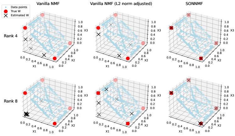
Figure 1: The reconstructed columns of $\bm{W}$ (cross) by NMF and SON-NMF together with the ground truth columns of $\bm{W}$ (red dots). Left: $\bm{W}$ given by NMF; middle: $\bm{W}$ given by NMF, with column normalized to 1. Right: $\bm{W}$ from SON-NMF. In both cases $r=4$ and $r=8$, the crosses given by SON-NMF fit numerically with the red dots.

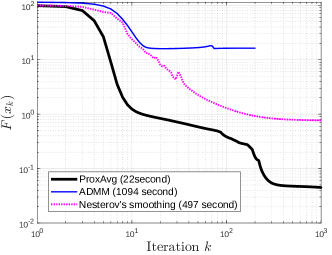
Figure 2: Righ: The convergence plot of SON-NMF cost function on synthetic data in experiment 2. Here we compare the convergence of three BCD algorithms with different method on solving the W-subproblem: proximal average (this work), ADMM and Nesterov’s smoothing. In the plot we also shows the computation time in second. The result here shows that compared with ADMM and smoothing, proximal average has the fastest convergence. Right: The score (the SON term) of selecting columns in $\bm{W}$ on the swimmer dataset, based on simple greedy search. The red line $r=17$ indicates a cut-off point, which is exactly the number of component in the dataset.

5.1.2 The swimmer dataset

Now we use the swimmer dataset introduced by [48]. The dataset consists of $256$ figures with each $20$-by-$11$ pixel of a skeleton body “swimming”, see the top row of Fig. 3. By inspection, the dataset consists of a rank-17 NMF: 1 for the torso, 16 for the 4 limbs with each limb corresponding to 4 different movement. A rank-50 (with $r=50>17=r^{*}$) SON-NMF is used in this dataset and we successfully recover all the 17 components. The redundant components are all captured as noise with small energy. Furthermore, if we perform a simple greedy search to determine the columns of $\bm{W}$ to be extracted, the right figure of Fig. 2 shows the score with a cut-off point exactly at $r=17$.

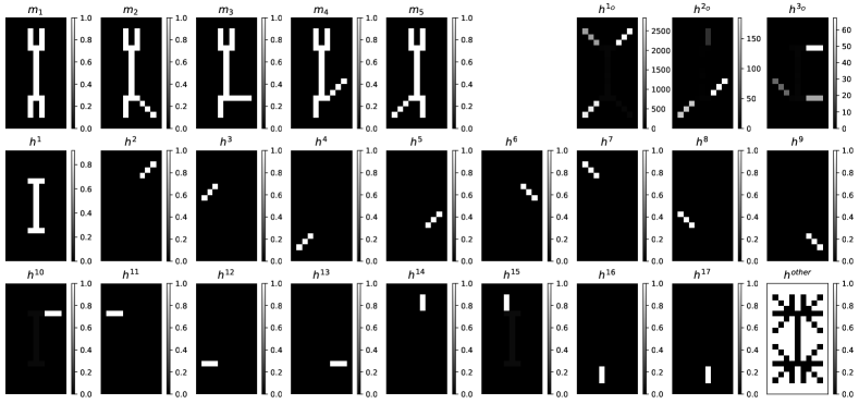
Figure 3: Top row, left: first 5 images ($\bm{m}^{1},\bm{m}^{2},\dots,\bm{m}^{5}$) in the swimmer dataset, showing a swimmer “swimming”. Top row, right: 3 $\bm{h}^{j}_{\text{O}}$ obtained from rank-50 vanilla NMF, where the subscript in $\bm{h}^{j}_{\text{O}}$ denotes the standard NMF. We can see that $\bm{h}^{j}_{\text{O}}$ contains mixed result. Bottom rows: The decomposition result of rank-50 SON-NMF. Here $\bm{h}^{1}$ captures the torso, $\bm{h}^{2},\bm{h}^{3},\dots,\bm{h}^{17}$ capture the four limbs, and $\bm{h}^{\text{other}}$, which denotes the sum of all the other components, represent the noise, with a clear illustration that $\bm{h}^{\text{other}}$ is complementary to all $\bm{h}^{1},\dots,\bm{h}^{17}$. We remark that the $\bm{w}$ corresponding to $\bm{h}^{\text{other}}$ has a very small energy (not plotted here). For the full decomposition result of the vanilla NMF, see appendix.

5.1.3 Jasper ridge hyperspectral dataset

In this section we conduct experiment on the Jasper Ridge dataset, which is a $100$-by-$100$-by-$198$ dataset with pixel dimensions $100\times 100$ (number of pixels in each row and each column) and wavelength dimension of $198$ (the dataset consists of 198 bandwidth of wavelengths). We refer to [2, Section 1.3.2] for the background of applying NMF on hyperspectral image. Fig.4 shows the photo of the Jasper Ridge and the three regions used in experiments. We remark that, due to the large numerical value of the entries of the dataset, we have to scale $\lambda$ (the SON regularization parameter) to a large value (as shown in Table 1).

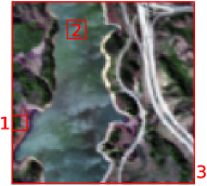
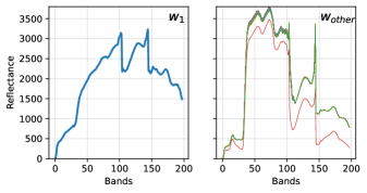
Figure 4: Left: The photo of the Jasper Ridge dataset, with the three regions of the dataset used in three experiments labeled in red. Right: Result for Jasper experiment 1. SON-NMF identifies the two material: soil ($\bm{w}_{1}$) and vegetation ($\bm{w}_{\text{other}}$, refers to all the columns in $\bm{W}$ except $\bm{w}_{1}$).

Jasper experiment 1

We run a rank-$64$ SON-NMF on a $8$-by-$8$ region consists of vegetation and soil. Gere we use $r=64=mn$ in SON-NMF, where $r$ is as large as the size of the dataset. Fig.4 shows the matrix $\bm{W}$ obtained from the SON-NMF. By inspection, region 1 consists of two end-member material: soil and vegetation. SON-NMF identified the two material, see Fig.4. This experiment showcases the ability of SON-NMF to correctly identify the correct number of components in the data without knowing the factorization rank.

Jasper experiment 2

We run a rank-$100$ SON-NMF on a $10$-by-$10$ water region. This region contains only water so it expected there is only one component in the decomposition. SON-NMF successfully identify the water component from the data and reduced a rank$-100$ NMF to a rank-1 NMF.

We remark that, by Perron-Frobenius theorem, the rank-1 solution here can also be obtained algebraically by the leading component in the eigendecomposition of the covariance matrix of the data. I.e., we have exact solution for rank-1 NMF by eigendecomposition, see the following proposition.

Proposition 1.

Given a data matrix $\bm{M}\in\mathbb{R}^{m\times n}_{+}$ and assume $\bm{M}=\bm{W}\bm{H}$ is the NMF of $\bm{M}$. Assume the columns of $\bm{W}$, denoted by $\bm{w}_{j}$, is ordered according to the norm of $\bm{w}_{j}\bm{h}^{j}$ contributing to $\bm{M}$. Then, for the case $r=1$ (the data has a rank-1 NMF), the vector $\bm{w}_{1}$ (the leading column of $\bm{W}$) can be given by the leading eigenvector of the eigendecomposition of $\bm{M}\bm{M}^{\top}$.

Proof.

By $\bm{M}=\bm{W}\bm{H}$ we have $\bm{M}\bm{M}^{\top}=\bm{W}\bm{H}\bm{H}^{\top}\bm{W}^{\top}=\bm{W}\bm{G}\bm{W}^{\top}$ where $\bm{G}\coloneqq\bm{H}\bm{H}^{\top}$. Let the eigendecomposition of $\bm{G}$ and $\bm{M}\bm{M}^{\top}$ as $\bm{G}=\bm{V}\bm{\Sigma}\bm{V}^{\top}$ and $\bm{M}\bm{M}^{\top}=\bm{U}\bm{\Lambda}\bm{U}^{\top}$. Then

$$\bm{W}\bm{V}\bm{\Sigma}\bm{V}^{\top}\bm{W}^{\top}=\bm{U}\bm{\Lambda}\bm{U}^{\top}\leavevmode\nobreak\ \implies\leavevmode\nobreak\ \bm{W}\bm{V}=\bm{U}\leavevmode\nobreak\ \implies\leavevmode\nobreak\ (\bm{W}\bm{V})_{:,1}=\bm{U}_{:,1}\leavevmode\nobreak\ \iff\leavevmode\nobreak\ \bm{W}\bm{v}_{1}=\bm{u}_{1}.$$

Both $\bm{G}=\bm{H}\bm{H}^{\top}$ and $\bm{M}\bm{M}^{\top}$ are nonnegative square matrices, by Perron-Frobenius theorem, both $\bm{u}_{1}$ and $\bm{v}_{1}$ are nonnegative vectors. Thus $\bm{W}\bm{v}_{1}=\bm{u}_{1}$ means $\bm{u}_{1}\in\textrm{cone}(\bm{W})$. Lastly $\bm{u}_{1}=\bm{w}_{1}$ if $\textrm{rank}(\bm{W})=1$. ∎

Fig.5 shows that the result obtained from SON-NMF agree with the exact solution provided by eigendecomposition, and has a relative error of $0.006$.

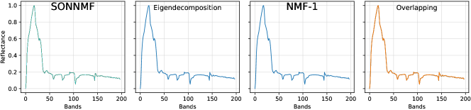
Figure 5: Result for Jasper experiment 2. The rank-100 SON-NMF (with $r=100$ that is much larger than the ground truth $r^{*}$) identifies the water spectrum in the decomposition. Left: the plotting of all the 100 columns in $\bm{w}$ share the same waveform. The middle two figures: the $\bm{W}$ obtained by eigendecomposition and rank-1 vanilla NMF. Right: the plot of overlapping all the $\bm{W}$, showing that SON-NMF is producing result agreeing with vanilla NMF. For clarification we have normalized all the $\bm{w}$ here to unit $\ell_{\infty}$-norm.

Jasper experiment 3

In this experiment, we run a rank-$20$ SON-NMF on the whole Jasper Ridge dataset. Four material are extracted, see Fig.6. The materials extracted agree with the results obtained from other methods.

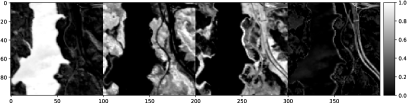
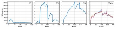
Figure 6: Result for Jasper experiment 3. Four material are extracted: (from left to right) water, vegetation, soil and road.

5.1.4 The Urban hyperspectral dataset

In this section we conduct experiment on big data with $1.5\times 10^{7}$ data points. We use a dataset named Urban that is a 307-by-307-by-162 data cube with pixel dimensions 307-by-307 (number of pixels in each row and each column) and wavelength dimension of 162 (the dataset consists of 162 bandwidth of wavelengths). We run a rank-20 SON-NMF with the following parameters: $\lambda=\gamma=10^{6}$. We run at most 1000 iterations. SON-NMF successfully identified 5 clusters of material, see Fig.7.

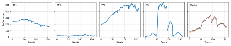
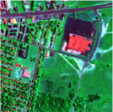
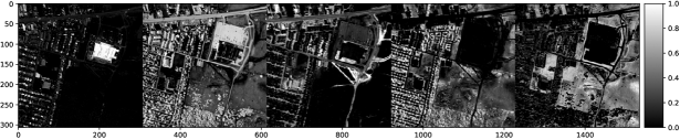
Figure 7: The reconstruction of a rank-20 SON-NMF on the Urban dataset. Here SON-NMF identified 5 clusters of material: (from left to right) roof, asphalt, soil, tree, and grass. Bottom left: the photo of the Urban dataset. We remark that the weak component asphalt in the dataset, is extracted by the SON-NMF. This is not the case by the classical NMF or with other rank estimation appraoch.

5.2 Speed of the algorithm

In Fig. 2 we showed the convergence of the BCD (Algorithm 1) with proximal average on solving the W-subproblem (Algorithm 3) compared with BCD with ADMM to solve the W-subproblem and BCD with Nesterov’s smoothing to solve the W-subproblem. The result shown in Fig. 2 tells that proximal average has the best performance. We refer the reader to [25] for the discussion why proximal average preforms better than smoothing. In the following we discuss why proximal average perform much better than ADMM.

Why ADMM is not suitable for SON-NMF: expensive per-iteration cost

Problem (8) with problem size $n\times 1$ can be solved by multi-block ADMM, which introduces $N$ auxiliary variables and $N$ Lagrangian multipliers, and the augmented Lagrangian has a problem size of $n\times(1+2N)$. Such explosion of size makes the ADMM expensive for designing fast algorithm. To be exact, $\bm{W}\mapsto P(\bm{W})$ is a $m$-by-$r$ to $m$-by-$r(r-1)/2$ mapping, i.e., there are many nonsmooth terms $\|\bm{w}_{i}-\bm{w}_{j}\|_{2}$ in SON. For each $\bm{w}_{i}$, the number of non-smooth terms in the optimization subproblem is $r$, and thus for the multi-block ADMM, the per-iteration complexity for each subproblem is $m(1+2r)$, and for all the $r$ columns in $\bm{W}$, the multi-block ADMM has a per-iteration complexity of $\mathcal{O}(2mr^{2}+mr)$. In contrast, proximal-average has a per-iteration complexity of $\mathcal{O}(mr)$. In this work $r$ is possibly as large as $m$, hence a per-iteration complexity of $\mathcal{O}(2mr^{2}+mr)\big{|}_{r=m}=\mathcal{O}(2m^{3}+m^{2})$ for ADMM is very expensive for solving the $\bm{W}$-subproblem, compared to a $\mathcal{O}(mr)\big{|}_{r=m}=\mathcal{O}(m^{2})$ cost for proximal-average. Furthermore, it is well known that ADMM has a slow convergence and therefore it may take even more iterations to solve SON-NMF.

5.3 Discussion: favourable features of SON-NMF for applications

Lastly we discuss favourable features of SON-NMF for applications that we have shown or observed.

Is empirically rank-revealing

All the seven experiments in section 5 shows that SON-NMF can effectively learn the rank of the NMF without prior knowledge.

Can deal with rank deficiency

SON-NMF is especially good at dealing with dataset with rank deficiency. This ability is not presented in othe regularized NMF model such as minvol NMF [3], which also have an empirically rank-revealing ability.

Can detect weak component in the dataset

Due to the clustering nature of the SON term, SON-NMF is better at detecting weak component in the dataset than the vanilla NMF.

• In the Jasper dataset in section 5, the water component has small energy relative to other components: it only contribute to $\|\bm{w}_{\text{water}}\bm{h}^{\text{water}}\|_{F}/\|\bm{M}\|_{F}=9\%$ energy in the dataset, compared with 54% for the vegetation (tree/grass) component.

• The squared-F-norm in the expression $\|\bm{M}-\bm{W}\bm{H}\|_{F}^{2}$ will raise the importance of the large energy component in NMF, and thus making the algorithm emphasizing large component in the iteration and ignoring the weak component.

Thus, with $r=4$, the vanilla NMF failed to extract the water component (see the full result in the Appendix). However, for SON-NMF, as the cost function contains the term $\|\bm{w}_{\text{other}}-\bm{w}_{\text{water}}\|_{2}$, SON-NMF will extract the water component.

The ability of SON-NMF to extract weak component is also supported by Lemma 1 that the smallest possible cluster size of any cluster identified in the SON term is bounded below by 1.

Can handle spectral variability

Note that the solutions of SON-NMF hyperspectral images (i.e., the $\bm{W}$ plots in both Fig.4, Fig.5, Fig.6, Fig.7) exhibit the phenomenon of spectral variability [49], and hence we argue that SON-NMF can be potentially useful in hyperspectral imaging: instead of using a sophisticated data processing pipeline as described in [49], SON alone is enough to deal with the spectral variability.

Is a hierarchically clustering

In the case of SON clustering, different values of the regularization parameter $\lambda$ yield different numbers of clusters. This is beneficial for dataset that is hierarchically clustered, so that one value of $\lambda$ yields the coarse clustering while another yields the finer clustering. In the experiments on hyperspectral images, different values of $\lambda$ give different but useful results.

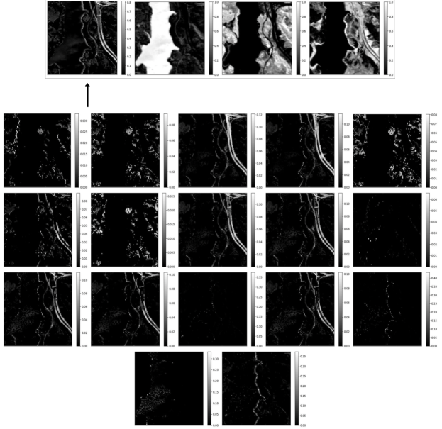
Figure 8: The full decomposition map of SON-NMF ($r=20$) on Jasper dataset (with $r^{*}$ expected to be around $4$). Here the road endmember consists of $17$ components.

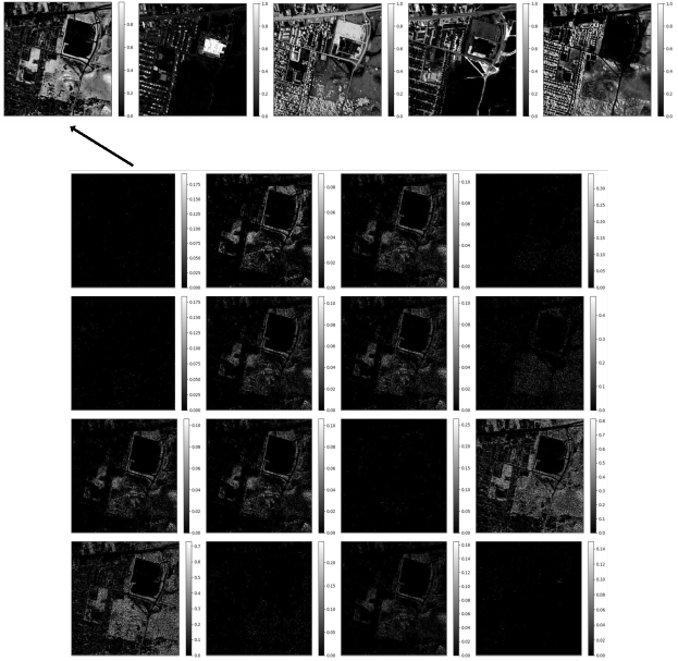
Figure 9: The full decomposition map of SON-NMF ($r=20$) on urban dataset (with $r^{*}$ expected to be around $5$). Here the grass endmember consists of $16$ components.

6 Conclusion

In this paper we proposed a sum-of-norm regularized NMF model, aimed at estimating the rank in NMF on-the-fly. The proposed SON-NMF is a nonconvex nonsmooth non-separable non-proximal optimization problem, and we develope a BCD algorithm with proximal-average for solving SON-NMF. Theoretically we show that the complexity of the SON term in SON-NMF is irreducible, meaning that the complexity of solving SON-NMF is possibly very high. This is expected since rank estimation is an NP-hard problem in NMF. Lastly we empirically show that SON-NMF is capable to detect the correct factorization rank in NMF, and potentially applicable to imaging applications with some favourable features.

Additional experimental results

Vanilla NMF on the swimmer dataset

Fig. 10 shows the decomposition result of swimmer dataset by rank-50 vanilla NMF.

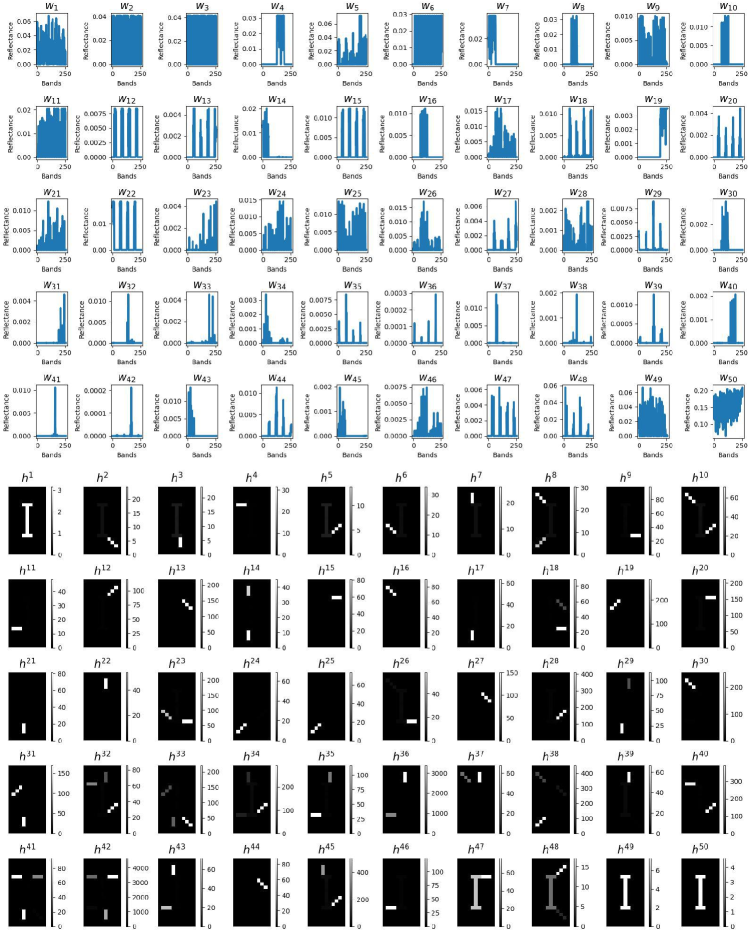
Figure 10: The decomposition result of the swimmer dataset by rank-50 vanilla NMF. We can see that the result do not produce component-wise decomposition, the limbs and torsos are mixed. Furthermore, each limb is represented by several component. For example, $h^{17}$ and $h^{21}$ represent the same left leg.

Vanilla NMF on the Jasper dataset

Fig. 11 shows the decomposition result of the full Jasper dataset by rank-20 vanilla NMF.

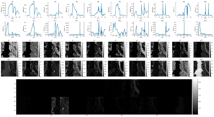
Figure 11: The decomposition result of the full Jasper dataset by rank-20 vanilla NMF. We can see that the result do not produce naturally-looking spectrum for $\bm{W}$ for many components. Compared with SON-NMF, the water component is not separated from other components, meaning that vanilla NMF failed to separate water component from other material.

Vanilla NMF on the Urban dataset

Fig. 12 shows the decomposition result of the full Urban dataset by rank-20 vanilla NMF.

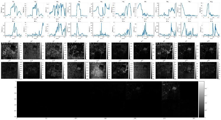
Figure 12: The decomposition result of the full Urban dataset by rank-20 vanilla NMF. We can see that the result do not produce naturally-looking spectrum for $\bm{W}$ for many components.

References

- [1] P. Paatero and U. Tapper, “Positive matrix factorization: A non-negative factor model with optimal utilization of error estimates of data values,” Environmetrics, vol. 5, no. 2, pp. 111–126, 1994.
- [2] N. Gillis, Nonnegative matrix factorization. SIAM, 2020.
- [3] V. Leplat, A. M. Ang, and N. Gillis, “Minimum-volume rank-deficient nonnegative matrix factorizations,” in ICASSP 2019-2019 IEEE International Conference on Acoustics, Speech and Signal Processing (ICASSP), pp. 3402–3406, IEEE, 2019.
- [4] A. Berman and R. J. Plemmons, Nonnegative matrices in the mathematical sciences. SIAM, 1994.
- [5] V. Leplat, N. Gillis, and A. M. Ang, “Blind audio source separation with minimum-volume beta-divergence nmf,” IEEE Transactions on Signal Processing, vol. 68, pp. 3400–3410, 2020.
- [6] M. S. Ang, “Nonnegative matrix and tensor factorizations: Models, algorithms and applications,” Ph. D. thesis, 2020.
- [7] S. A. Vavasis, “On the complexity of nonnegative matrix factorization,” SIAM Journal on Optimization, vol. 20, no. 3, pp. 1364–1377, 2010.
- [8] M. Udell and A. Townsend, “Why are big data matrices approximately low rank?,” SIAM Journal on Mathematics of Data Science, vol. 1, no. 1, pp. 144–160, 2019.
- [9] V. Y. Tan and C. Févotte, “Automatic relevance determination in nonnegative matrix factorization with the -divergence,” IEEE transactions on pattern analysis and machine intelligence, vol. 35, no. 7, pp. 1592–1605, 2012.
- [10] F. Esposito, A. Boccarelli, and N. Del Buono, “An NMF-Based Methodology for Selecting Biomarkers in the Landscape of Genes of Heterogeneous Cancer-Associated Fibroblast Populations,” Bioinformatics and Biology Insights, vol. 14, p. 1177932220906827, 2020.
- [11] S. Squires, A. Prügel-Bennett, and M. Niranjan, “Rank selection in nonnegative matrix factorization using minimum description length,” Neural computation, vol. 29, no. 8, pp. 2164–2176, 2017.
- [12] J. E. Cohen and U. G. Rothblum, “Nonnegative ranks, decompositions, and factorizations of nonnegative matrices,” Linear Algebra and its Applications, vol. 190, pp. 149–168, 1993.
- [13] J. Dewez, N. Gillis, and F. Glineur, “A geometric lower bound on the extension complexity of polytopes based on the f-vector,” Discrete Applied Mathematics, vol. 303, pp. 22–38, 2021.
- [14] S. F. Cotter, B. D. Rao, K. Engan, and K. Kreutz-Delgado, “Sparse solutions to linear inverse problems with multiple measurement vectors,” IEEE Transactions on Signal Processing, vol. 53, no. 7, pp. 2477–2488, 2005.
- [15] F. Nie, H. Huang, X. Cai, and C. Ding, “Efficient and robust feature selection via joint 2, 1-norms minimization,” Advances in neural information processing systems, vol. 23, 2010.
- [16] D. Kong, C. Ding, and H. Huang, “Robust nonnegative matrix factorization using l21-norm,” in Proceedings of the 20th ACM international conference on Information and knowledge management, pp. 673–682, 2011.
- [17] D. Cai, X. He, J. Han, and T. S. Huang, “Graph regularized nonnegative matrix factorization for data representation,” IEEE transactions on pattern analysis and machine intelligence, vol. 33, no. 8, pp. 1548–1560, 2010.
- [18] D. E. Farrar and R. R. Glauber, “Multicollinearity in regression analysis: the problem revisited,” The Review of Economic and Statistics, pp. 92–107, 1967.
- [19] M. A. Ang and N. Gillis, “Volume regularized non-negative matrix factorizations,” in 2018 9th Workshop on Hyperspectral Image and Signal Processing: Evolution in Remote Sensing (WHISPERS), pp. 1–5, IEEE, 2018.
- [20] P. Tseng and S. Yun, “A coordinate gradient descent method for nonsmooth separable minimization,” Mathematical Programming, vol. 117, pp. 387–423, 2009.
- [21] Y. Xu and W. Yin, “A block coordinate descent method for regularized multiconvex optimization with applications to nonnegative tensor factorization and completion,” SIAM Journal on imaging sciences, vol. 6, no. 3, pp. 1758–1789, 2013.
- [22] M. Razaviyayn, M. Hong, and Z.-Q. Luo, “A unified convergence analysis of block successive minimization methods for nonsmooth optimization,” SIAM Journal on Optimization, vol. 23, no. 2, pp. 1126–1153, 2013.
- [23] J. Bolte, S. Sabach, and M. Teboulle, “Proximal alternating linearized minimization for nonconvex and nonsmooth problems,” Mathematical Programming, vol. 146, no. 1-2, pp. 459–494, 2014.
- [24] H. Le, N. Gillis, and P. Patrinos, “Inertial block proximal methods for non-convex non-smooth optimization,” in International Conference on Machine Learning, pp. 5671–5681, PMLR, 2020.
- [25] Y.-L. Yu, “Better approximation and faster algorithm using the proximal average,” Advances in neural information processing systems, vol. 26, 2013.
- [26] H. H. Bauschke, R. Goebel, Y. Lucet, and X. Wang, “The proximal average: basic theory,” SIAM Journal on Optimization, vol. 19, no. 2, pp. 766–785, 2008.
- [27] A. M. S. Ang and N. Gillis, “Algorithms and comparisons of nonnegative matrix factorizations with volume regularization for hyperspectral unmixing,” IEEE Journal of Selected Topics in Applied Earth Observations and Remote Sensing, vol. 12, no. 12, pp. 4843–4853, 2019.
- [28] K. Pelckmans, J. De Brabanter, J. A. Suykens, and B. De Moor, “Convex clustering shrinkage,” in PASCAL workshop on statistics and optimization of clustering workshop, 2005.
- [29] F. Lindsten, H. Ohlsson, and L. Ljung, “Clustering using sum-of-norms regularization: With application to particle filter output computation,” in 2011 IEEE Statistical Signal Processing Workshop (SSP), pp. 201–204, IEEE, 2011.
- [30] T. D. Hocking, A. Joulin, F. Bach, and J.-P. Vert, “Clusterpath: an algorithm for clustering using convex fusion penalties,” in 28th international conference on machine learning, p. 1, 2011.
- [31] L. Niu, R. Zhou, Y. Tian, Z. Qi, and P. Zhang, “Nonsmooth penalized clustering via regularized sparse regression,” IEEE transactions on cybernetics, vol. 47, no. 6, pp. 1423–1433, 2016.
- [32] T. Jiang and S. Vavasis, “Certifying clusters from sum-of-norms clustering,” arXiv preprint arXiv:2006.11355, 2020.
- [33] X. Huang, A. Ang, J. Zhang, and Y. Wang, “Inhomogeneous graph trend filtering via a cardinality penalty,” arXiv preprint arXiv:2304.05223, 2023.
- [34] A. Beck, First-order methods in optimization. SIAM, 2017.
- [35] Y. Yuan, D. Sun, and K.-C. Toh, “An efficient semismooth newton based algorithm for convex clustering,” in International Conference on Machine Learning, pp. 5718–5726, PMLR, 2018.
- [36] J. Krarup and S. Vajda, “On torricelli’s geometrical solution to a problem of fermat,” IMA Journal of Management Mathematics, vol. 8, no. 3, pp. 215–224, 1997.
- [37] N. M. Nam, N. T. An, R. B. Rector, and J. Sun, “Nonsmooth algorithms and nesterov’s smoothing technique for generalized fermat–torricelli problems,” SIAM Journal on Optimization, vol. 24, no. 4, pp. 1815–1839, 2014.
- [38] G. Cantor, “Ueber eine elementare frage der mannigfaltigketislehre.,” Jahresbericht der Deutschen Mathematiker-Vereinigung, vol. 1, pp. 72–78, 1890.
- [39] C. Hildreth, “A quadratic programming procedure,” Naval research logistics quarterly, vol. 4, no. 1, pp. 79–85, 1957.
- [40] S. J. Wright, “Coordinate descent algorithms,” Mathematical programming, vol. 151, no. 1, pp. 3–34, 2015.
- [41] L. Condat, “Fast projection onto the simplex and the l1 ball,” Mathematical Programming, vol. 158, no. 1-2, pp. 575–585, 2016.
- [42] Y. Nesterov, Introductory lectures on convex optimization: A basic course, vol. 87. Springer Science & Business Media, 2003.
- [43] M. Schmidt, N. Roux, and F. Bach, “Convergence rates of inexact proximal-gradient methods for convex optimization,” Advances in neural information processing systems, vol. 24, 2011.
- [44] Y. Nesterov, “Smooth minimization of non-smooth functions,” Mathematical programming, vol. 103, pp. 127–152, 2005.
- [45] G. B. Passty, “Ergodic convergence to a zero of the sum of monotone operators in hilbert space,” Journal of Mathematical Analysis and Applications, vol. 72, no. 2, pp. 383–390, 1979.
- [46] M. Fukushima and H. Mine, “A generalized proximal point algorithm for certain non-convex minimization problems,” International Journal of Systems Science, vol. 12, no. 8, pp. 989–1000, 1981.
- [47] P. L. Combettes and V. R. Wajs, “Signal recovery by proximal forward-backward splitting,” Multiscale modeling & simulation, vol. 4, no. 4, pp. 1168–1200, 2005.
- [48] D. Donoho and V. Stodden, “When does non-negative matrix factorization give a correct decomposition into parts?,” Advances in neural information processing systems, vol. 16, 2003.
- [49] R. A. Borsoi, T. Imbiriba, J. C. M. Bermudez, C. Richard, J. Chanussot, L. Drumetz, J.-Y. Tourneret, A. Zare, and C. Jutten, “Spectral variability in hyperspectral data unmixing: A comprehensive review,” IEEE geoscience and remote sensing magazine, vol. 9, no. 4, pp. 223–270, 2021.